Geometric Wavelet Scattering Networks
on Compact Riemannian Manifolds

Abstract

The Euclidean scattering transform was introduced nearly a decade ago to improve the mathematical understanding of convolutional neural networks. Inspired by recent interest in geometric deep learning, which aims to generalize convolutional neural networks to manifold and graph-structured domains, we define a geometric scattering transform on manifolds. Similar to the Euclidean scattering transform, the geometric scattering transform is based on a cascade of wavelet filters and pointwise nonlinearities. It is invariant to local isometries and stable to certain types of diffeomorphisms. Empirical results demonstrate its utility on several geometric learning tasks. Our results generalize the deformation stability and local translation invariance of Euclidean scattering, and demonstrate the importance of linking the used filter structures to the underlying geometry of the data.

1 Introduction

In an effort to improve our mathematical understanding of deep convolutional networks and their learned features, Mallat (2010, 2012) introduced the scattering transform for signals on $\mathbb{R}^{d}$. This transform has an architecture similar to convolutional neural networks (ConvNets), based on a cascade of convolutional filters and simple pointwise nonlinearities. However, unlike many other deep learning methods, this transform uses the complex modulus as its nonlinearity and does not learn its filters from data, but instead uses designed filters. As shown in Mallat (2012), with properly chosen wavelet filters, the scattering transform is provably invariant to the actions of certain Lie groups, such as the translation group, and is also provably Lipschitz stable to small diffeomorphisms, where the size of a diffeomorphism is quantified by its deviation from a translation. These notions were applied in Bruna and Mallat (2011, 2013); Sifre and Mallat (2012, 2013, 2014); Oyallon and Mallat (2015) using groups of translations, rotations, and scaling operations, with applications in image and texture classification. Additionally, the scattering transform and its deep filter bank approach have also proven to be effective in several other fields, such as audio processing (Andén and Mallat, 2011, 2014; Wolf et al., 2014, 2015; Andén et al., 2019), medical signal processing (Chudácek et al., 2014), and quantum chemistry (Hirn et al., 2017; Eickenberg et al., 2017, 2018; Brumwell et al., 2018). Mathematical generalizations to non-wavelet filters have also been studied, including Gabor filters as in the short time Fourier transform (Czaja and Li, 2019) and more general classes of semi-discrete frames (Grohs et al., 2016; Wiatowski and Bölcskei, 2015, 2018).

However, many data sets of interest have an intrinsically non-Euclidean structure and are better modeled by graphs or manifolds. Indeed, manifold learning models (e.g., Tenenbaum et al., 2000; Coifman and Lafon, 2006a; van der Maaten and Hinton, 2008) are commonly used for representing high-dimensional data in which unsupervised algorithms infer data-driven geometries to capture intrinsic structure in data. Furthermore, signals supported on manifolds are becoming increasingly prevalent, for example, in shape matching and computer graphics. As such, a large body of work has emerged to explore the generalization of spectral and signal processing notions to manifolds (Coifman and Lafon, 2006b) and graphs (Shuman et al., 2013a, and references therein). In these settings, functions are supported on the manifold or the vertices of the graph, and the eigenfunctions of the Laplace-Beltrami operator, or the eigenvectors of the graph Laplacian, serve as the Fourier harmonics. This increasing interest in non-Euclidean data geometries has led to a new research direction known as geometric deep learning, which aims to generalize convolutional networks to graph and manifold structured data (Bronstein et al., 2017, and references therein).

Inspired by geometric deep learning, recent works have also proposed an extension of the scattering transform to graph domains. These mostly focused on finding features that represent a graph structure (given a fixed set of signals on it) while being stable to graph perturbations. In Gama et al. (2019b), a cascade of diffusion wavelets from Coifman and Maggioni (2006) was proposed, and its Lipschitz stability was shown with respect to a global diffusion-inspired distance between graphs. These results were generalized in Gama et al. (2019a) to graph wavelets constructed from more general graph shift operators. A similar construction discussed in Zou and Lerman (2019) was shown to be stable to permutations of vertex indices, and to small perturbations of edge weights. Gao et al. (2019) established the viability of graph scattering coefficients as universal graph features for data analysis tasks (e.g., in social networks and biochemistry data). The wavelets used in Gao et al. (2019) are similar to those used in Gama et al. (2019b), but are constructed from an asymmetric lazy random walk matrix (the wavelets in Gama et al. (2019b) are constructed from a symmetric matrix). The constructions of Gama et al. (2019b) and Gao et al. (2019) were unified in Perlmutter et al. (2019), which introduced a large family of graph wavelets, including both those from Gama et al. (2019b) and Gao et al. (2019) as special cases, and showed that the resulting scattering transforms enjoyed many of the same theoretical properties as in Gama et al. (2019b).

In this paper we consider the manifold aspect of geometric deep learning. There are two basic tasks in this setting: (1) classification of multiple signals over a single, fixed manifold; and (2) classification of multiple manifolds. Beyond these two tasks, there are additional problems of interest such as manifold alignment, partial manifold reconstruction, and generative models. Fundamentally for all of these tasks, both in the approach described here and in other papers, one needs to process signals over a manifold. Indeed, even in manifold classification tasks and related problems such as manifold alignment, one often begins with a set of universal features that can be defined on any manifold, and which are processed in such a way that allows for comparison of two or more manifolds. In order to carry out these tasks, a representation of manifold supported signals needs to be stable to orientations, noise, and deformations over the manifold geometry. Working towards these goals, we define a scattering transform on compact smooth Riemannian manifolds without boundary, which we call geometric scattering. Our construction is based on convolutional filters defined spectrally via the eigendecomposition of the Laplace-Beltrami operator over the manifold, as discussed in Section 2. We show that these convolutional operators can be used to construct a wavelet frame similar to the diffusion wavelets constructed in Coifman and Maggioni (2006). Then, in Section 3, we construct a cascade of these generalized convolutions and pointwise absolute value operations that is used to map signals on the manifold to scattering coefficients that encode approximate local invariance to isometries, which correspond to translations, rotations, and reflections in Euclidean space. We then show in Section 4 that our scattering coefficients are also stable to the action of diffeomorphisms with a notion of stability analogous to the Lipschitz stability considered in Mallat (2012) on Euclidean space. Our results provide a path forward for utilizing the scattering mathematical framework to analyze and understand geometric deep learning, while also shedding light on the challenges involved in such generalization to non-Euclidean domains. Indeed, while these results are analogous to those obtained for the Euclidean scattering transform, we emphasize that the underlying mathematical techniques are derived from spectral geometry, which plays no role in the Euclidean analysis. Numerical results in Section 5 show that geometric scattering coefficients achieve competitive results for signal classification on a single manifold, and classification of different manifolds. We demonstrate the geometric scattering method can capture the both local and global features to generate useful latent representations for various downstream tasks. Proofs of technical results are provided in the appendices.

1.1 Notation

Let $\mathcal{M}$ denote a compact, smooth, connected $d$-dimensional Riemannian manifold without boundary contained in $\mathbb{R}^{n}$, and let $\mathbf{L}^{2}(\mathcal{M})$ denote the set of functions $f:\mathcal{M}\rightarrow\mathbb{R}$ that are square integrable with respect to the Riemannian volume $dx.$ Let $r(x,x^{\prime})$ denote the geodesic distance between two points, and let $\Delta$ denote the Laplace-Beltrami operator on $\mathcal{M}$. Let $\mathrm{Isom}(\mathcal{M},\mathcal{M}^{\prime})$ denote the set of all isometries between two manifolds $\mathcal{M}$ and $\mathcal{M}^{\prime}$, and set $\mathrm{Isom}(\mathcal{M})=\mathrm{Isom}(\mathcal{M},\mathcal{M})$ to be the isometry group of $\mathcal{M}$. Likewise, we set $\mathrm{Diff}(\mathcal{M})=\mathrm{Diff}(\mathcal{M},\mathcal{M})$ to be the diffeomorphism group on $\mathcal{M}$. For $\zeta\in\mathrm{Diff}(\mathcal{M})$, we let $\|\zeta\|_{\infty}\coloneqq\sup_{x\in\mathcal{M}}r(x,\zeta(x))$ denote its maximum displacement.

2 Geometric wavelet transforms on manifolds

The Euclidean scattering transform is constructed using wavelet and low-pass filters defined on $\mathbb{R}^{d}$. In Section 2.1, we extend the notion of convolution against a filter (wavelet, low-pass, or otherwise), to manifolds using notions from spectral geometry. Many of the notions described in this section are geometric analogues of similar constructions used in graph signal processing (Shuman et al., 2013b). Section 2.2 utilizes these constructions to define Littlewood-Paley frames for $\mathbf{L}^{2}(\mathcal{M})$, and Section 2.3 describes a specific class of Littlewood-Paley frames which we call geometric wavelets.

2.1 Convolution on manifolds

On $\mathbb{R}^{d},$ the convolution of a signal $f\in\mathbf{L}^{2}(\mathbb{R}^{d})$ with a filter $h\in\mathbf{L}^{2}(\mathbb{R}^{d})$ is defined by translating $h$ against $f$; however, translations are not well-defined on generic manifolds. Nevertheless, convolution can also be characterized using the Fourier convolution theorem, i.e., $\widehat{f\ast h}(\omega)=\widehat{f}(\omega)\widehat{h}(\omega)$. Fourier analysis can be defined on $\mathcal{M}$ using the spectral decomposition of $-\Delta$. Since $\mathcal{M}$ is compact and connected, $-\Delta$ has countably many eigenvalues which we enumerate as $0=\lambda_{0}<\lambda_{1}\leq\lambda_{2}$ (repeating those with multiplicity greater than one), and there exists a sequence of eigenfunctions $\varphi_{0},\varphi_{1},\varphi_{2},\ldots$ such that $\{\varphi_{k}\}_{k\geq 0}$ is an orthonormal basis for $\mathbf{L}^{2}(\mathcal{M})$ and $-\Delta\varphi_{k}=\lambda_{k}\varphi_{k}.$ While one can take each $\varphi_{k}$ to be real valued, we do not assume this choice of eigenbasis. One can show that $\varphi_{0}$ is constant, which implies, by orthogonality, that $\varphi_{k}$ has mean zero for $k\geq 1.$ We consider the eigenfunctions $\{\varphi_{k}\}_{k\geq 0}$ as the Fourier modes of the manifold $\mathcal{M}$, and define the Fourier series $\widehat{f}\in\bm{\ell}^{2}$ of $f\in\mathbf{L}^{2}(\mathcal{M})$ as

$$\widehat{f}(k)\coloneqq\langle f,\varphi_{k}\rangle=\int_{\mathcal{M}}f(y)\overline{\varphi_{k}(y)}\,dy\,.$$

Since $\varphi_{0},\varphi_{1},\varphi_{2},\ldots$ form an orthonormal basis, we have

$$f(x)=\sum_{k\geq 0}\langle f,\varphi_{k}\rangle\varphi_{k}(x)=\sum_{k\geq 0}\widehat{f}(k)\varphi_{k}(x)=\sum_{k\geq 0}\left(\int_{\mathcal{M}}f(y)\overline{\varphi_{k}(y)}\,dy\right)\varphi_{k}(x)\,.$$ (1)

For $f,h\in\mathbf{L}^{2}(\mathcal{M}),$ we define the convolution $\ast$ over $\mathcal{M}$ between $f$ and $h$ as

$$f\ast h(x)\coloneqq\sum_{k\geq 0}\widehat{f}(k)\widehat{h}(k)\varphi_{k}(x)\,.$$ (2)

We let $T_{h}:\mathbf{L}^{2}(\mathcal{M})\rightarrow\mathbf{L}^{2}(\mathcal{M})$ be the corresponding operator $T_{h}f(x)\coloneqq f\ast h(x)$ and note that we may write

$$T_{h}f(x)=f\ast h(x)=\int_{\mathcal{M}}\left(\sum_{k\geq 0}\widehat{h}(k)\varphi_{k}(x)\overline{\varphi_{k}(y)}\right)f(y)\,dy=\int_{\mathcal{M}}K_{h}(x,y)f(y)\,dy\,,$$

where

$$K_{h}(x,y):=\sum_{k\geq 0}\widehat{h}(k)\varphi_{k}(x)\overline{\varphi_{k}(y)}\,.$$

It is well known that convolution on $\mathbb{R}^{d}$ commutes with translations. This equivariance property is fundamental to Euclidean ConvNets, and has spurred the development of equivariant neural networks on other spaces, e.g., Cohen and Welling (2016); Kondor and Trivedi (2018); Thomas et al. (2018); Kondor et al. (2018a); Cohen et al. (2018); Kondor et al. (2018b); Weiler et al. (2018). Since translations are not well-defined on $\mathcal{M},$ we instead seek to construct a family of operators which commute with isometries. Towards this end, we say a filter $h\in\mathbf{L}^{2}(\mathcal{M})$ is a spectral filter if $\lambda_{k}=\lambda_{\ell}$ implies $\widehat{h}(k)=\widehat{h}(\ell).$ In this case, there exists a function $H:[0,\infty)\rightarrow\mathbb{R}$, which we refer to as the spectral function of $h,$ such that

$$H(\lambda_{k})=\widehat{h}(k)\,,\quad\text{for all }k\geq 0\,.$$

In the proofs of our theorems, it will be convenient to group together eigenfunctions belonging to the same eigenspace. This motivates us to define

$$\Lambda\coloneqq\{\lambda\in\mathbb{R}:\text{ there exists }\varphi\in\mathbf{L}^{2}(\mathcal{M})\text{ such that }-\Delta\varphi=\lambda\varphi\}$$

as the set of all eigenvalues of $-\Delta,$ and to let

$$K^{(\lambda)}(x,y)\coloneqq\sum_{\lambda_{k}=\lambda}\varphi_{k}(x)\overline{\varphi_{k}(y)}$$ (3)

for each $\lambda\in\Lambda.$ We note that if $h$ is a spectral filter, then we may write

$$K_{h}(x,y)=\sum_{k\geq 0}H(\lambda_{k})\varphi_{k}(x)\overline{\varphi_{k}(y)}=\sum_{\lambda\in\Lambda}H(\lambda)K^{(\lambda)}(x,y)\,.$$ (4)

For a diffeomorphism $\zeta\in\mathrm{Diff}(\mathcal{M})$ we define the operator $V_{\zeta}:\mathbf{L}^{2}(\mathcal{M})\rightarrow\mathbf{L}^{2}(\mathcal{M})$ as

$$V_{\zeta}f(x)\coloneqq f(\zeta^{-1}(x))\,.$$

The operator $V_{\zeta}$ deforms the function $f\in\mathbf{L}^{2}(\mathcal{M})$ according to the diffeomorphism $\zeta$ of the underlying manifold $\mathcal{M}$. The following theorem shows that $T_{h}$ and $V_{\zeta}$ commute if $\zeta$ is an isometry and $h$ is a spectral filter. We note the assumption that $h$ is a spectral filter is critical and in general $T_{h}$ does not commute with isometries if $h$ is not a spectral filter. The proof is in Appendix A.

[]thmisoequi For every spectral filter $h\in\mathbf{L}^{2}(\mathcal{M})$ and for every $f\in\mathbf{L}^{2}(\mathcal{M})$,

$$T_{h}V_{\zeta}f=V_{\zeta}T_{h}f\,,\quad\forall\,\zeta\in\mathrm{Isom}(\mathcal{M})\,.$$

2.2 Littlewood-Paley frames over manifolds

A family of spectral filters $\{h_{\gamma}:\gamma\in\Gamma\}$ (with $\Gamma$ countable), is called a Littlewood-Paley frame if it satisfies the following condition which implies that the $h_{\gamma}$ cover the frequencies of $\mathcal{M}$ evenly:

$$\sum_{\gamma\in\Gamma}|\widehat{h}_{\gamma}(k)|^{2}=1\,,\quad\forall\,k\geq 0\,.$$ (5)

We define the corresponding frame analysis operator, $\mathcal{H}:\mathbf{L}^{2}(\mathcal{M})\rightarrow\bm{\ell}^{2}(\mathbf{L}^{2}(\mathcal{M}))$, by

$$\mathcal{H}f\coloneqq\{f\ast h_{\gamma}:\gamma\in\Gamma\}\,.$$

The following proposition shows that if (5) holds, then $\mathcal{H}f$ preserves the energy of $f$.

[]proplpframe If $\{h_{\gamma}:\gamma\in\Gamma\}$ satisfies (5), then $\mathcal{H}:\mathbf{L}^{2}(\mathcal{M})\rightarrow\bm{\ell}^{2}(\mathbf{L}^{2}(\mathcal{M}))$ is an isometry, i.e.,

$$\|\mathcal{H}f\|_{2,2}^{2}\coloneqq\sum_{\gamma\in\Gamma}\|f\ast h_{\gamma}\|_{2}^{2}=\|f\|_{2}^{2}\,,\quad\forall\,f\in\mathbf{L}^{2}(\mathcal{M})\,.$$

The proof of Proposition 2.2 is nearly identical to the corresponding result in the Euclidean case. For the sake of completeness, we provide full details in Appendix B. Since the operator $\mathcal{H}$ is linear, Proposition 2.2 also shows the operator $\mathcal{H}$ is non-expansive, i.e., $\|\mathcal{H}f_{1}-\mathcal{H}f_{2}\|_{2,2}\leq\|f_{1}-f_{2}\|_{2}$. This property is directly related to the $\mathbf{L}^{2}$ stability of a ConvNet of the form $\sigma_{m}(\mathcal{H}_{m}(\sigma_{m-1}(\mathcal{H}_{m-1}\cdots\sigma_{1}(\mathcal{H}_{1}f)))$, where the $\sigma_{\ell}$ are nonlinear functions. Indeed, if all the frame analysis operators $\mathcal{H}_{\ell}$ and all the nonlinear operators $\sigma_{\ell}$ are non-expansive, then the entire network is non-expansive as well.

2.3 Geometric wavelet transforms on manifolds

The geometric wavelet transform is a special type of Littlewood-Paley frame analysis operator in which the filters group the frequencies of $\mathcal{M}$ into dyadic packets. A spectral filter $\phi\in\mathbf{L}^{2}(\mathcal{M})$ is said to be a low-pass filter if $\widehat{\phi}(0)=1$ and $|\widehat{\phi}(k)|$ is non-increasing with respect to $k$. Typically, $|\widehat{\phi}(k)|$ decays rapidly as $k$ grows large. Thus, a low-pass filtering, $T_{\phi}f\coloneqq f\ast\phi$, retains the low frequencies of $f$ while suppressing the high frequencies. A wavelet $\psi\in\mathbf{L}^{2}(\mathcal{M})$ is a spectral filter such that $\widehat{\psi}(0)=0$. Unlike low-pass filters, wavelets have no frequency response at $k=0,$ but are generally well localized in the frequency domain away from $k=0.$

We shall define a family of low-pass and a wavelet filters, using the difference between low-pass filters at consecutive dyadic scales, in a manner which mimics standard wavelet constructions (see, e.g., Meyer, 1993). Let $G:[0,\infty)\rightarrow\mathbb{R}$ be a non-negative, non-increasing function with $G(0)=1$. Define a low-pass spectral filter $\phi$ and its dilation at scale $2^{j}$ for $j\in\mathbb{Z}$ by:

$$\widehat{\phi}(k)\coloneqq G(\lambda_{k})\quad\text{and}\quad\widehat{\phi}_{j}(k):=G(2^{j}\lambda_{k})\,.$$

Given the dilated low-pass filters, $\{\widehat{\phi}_{j}\}_{j\in\mathbb{Z}},$ we defined our wavelet filters by

$$\widehat{\psi}_{j}(k)\coloneqq\Big{[}|\widehat{\phi}_{j-1}(k)|^{2}-|\widehat{\phi}_{j}(k)|^{2}\Big{]}^{1/2}\,.$$ (6)

For $J\in\mathbb{Z},$ we let $A_{J}f:=f\ast\phi_{J}$ and $\Psi_{j}f:=f\ast\psi_{j}.$ We then define the geometric wavelet transform as

$$W_{J}f\coloneqq\{A_{J}f\,,\,\Psi_{j}f:j\leq J\}=\{f\ast\phi_{J}\,,\,f\ast\psi_{j}:j\leq J\}\,.$$

The geometric wavelet transform extracts the low frequency, slow transitions of $f$ over $\mathcal{M}$ through $A_{J}f$, and groups the high frequency, sharp transitions of $f$ over $\mathcal{M}$ into different dyadic frequency bands via the collection $\{\Psi_{j}f:j\leq J\}$. The following proposition can be proved by observing that $\{\phi_{J}\,,\,\psi_{j}:j\leq J\}$ forms a Littlewood-Paley frame and applying Proposition 2.2. The proof is nearly identical to the corresponding result in the Euclidean case; however, we provide full details in Appendix C in order to help keep this paper self-contained.

[]propwaveisom For any $J\in\mathbb{Z}$, $W_{J}:\mathbf{L}^{2}(\mathcal{M})\rightarrow\bm{\ell}^{2}(\mathbf{L}^{2}(\mathcal{M}))$ is an isometry, i.e.,

$$\|W_{J}f\|_{2,2}=\|f\|_{2}\,,\quad\forall\,f\in\mathbf{L}^{2}(\mathcal{M})\,.$$

An important example is $G(\lambda)=e^{-\lambda}$. In this case the low-pass kernel $K_{\phi_{J}}$ is the heat kernel on $\mathcal{M}$ at diffusion time $t=2^{J}$, and the wavelet operators $\Psi_{j}$ are similar to the diffusion wavelets introduced in Coifman and Maggioni (2006). We also note that wavelet constructions similar to ours were used in Hammond et al. (2011) and Dong (2017). Figure 1 depicts these wavelets over manifolds from the FAUST data set (Bogo et al., 2014). Unlike many wavelets commonly used in computer vision, our wavelets are not directional. Indeed, on a generic manifold the concept of directional wavelets is not well-defined since the isometry group cannot be decomposed into translations, rotations, and reflections. Instead, our wavelets have a donut-like shape which is somewhat similar to the wavelet obtained by applying the Laplacian operator on $\mathbb{R}^{d}$ to a $d$-dimensional Gaussian.

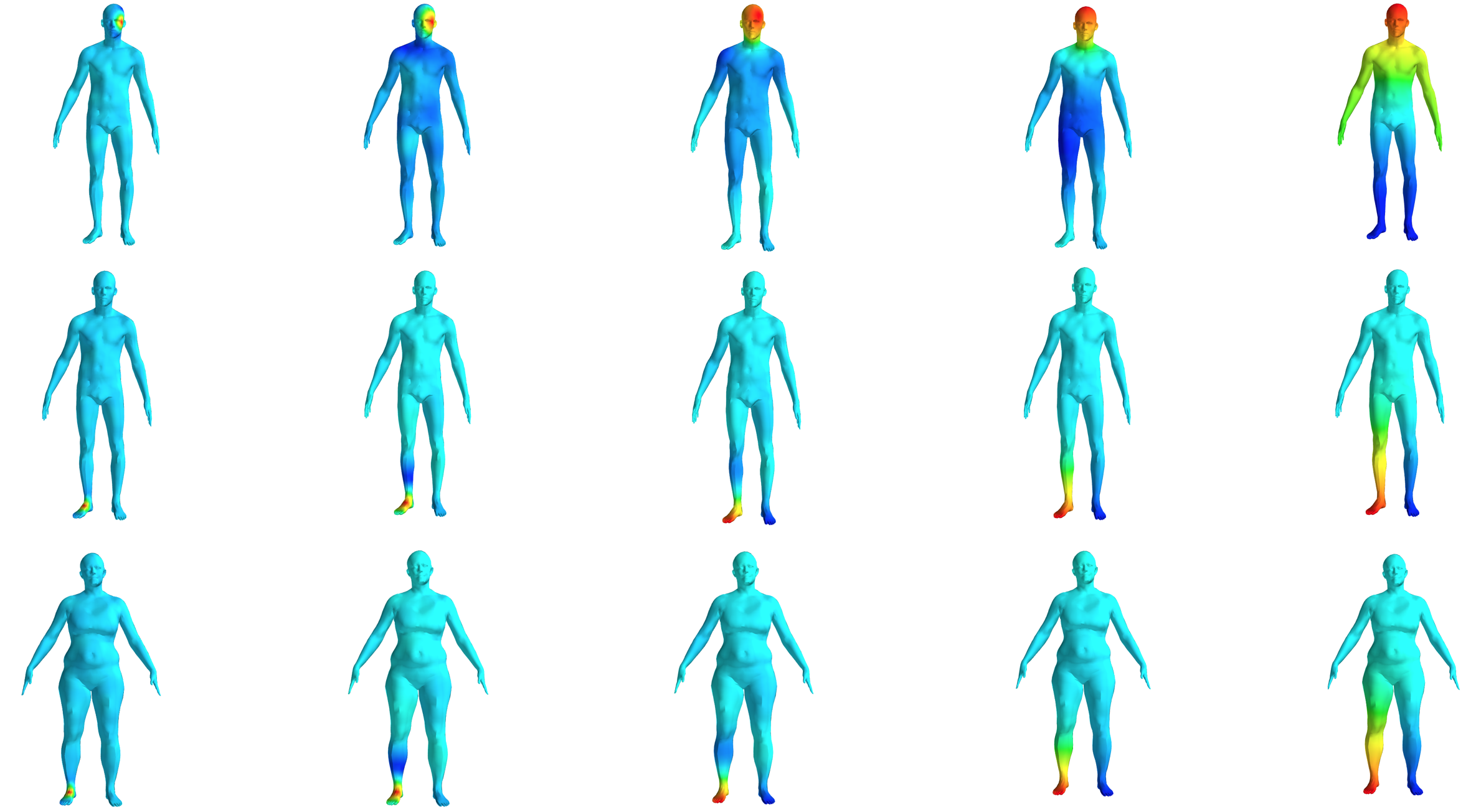
Figure 1: Geometric wavelets on the FAUST mesh with $G(\lambda)=e^{-\lambda}$. From left to right $j=-1,-3,-5,-7,-9$. Positive values are colored red, while negative values are dark blue.

3 The geometric wavelet scattering transform

The geometric wavelet scattering transform is a type of geometric ConvNet, constructed in a manner analogous to the Euclidean scattering transform (Mallat, 2012) as an alternating cascade of geometric wavelet transforms (defined in Section 2.3) and nonlinearities. As we shall show in Sections 3.3, 3.4, and 4, this transformation enjoys several desirable properties for processing data consisting of signals defined on a fixed manifold $\mathcal{M}$, in addition to tasks in which each data point is a different manifold and one is required to compare and classify manifolds. Tasks of the latter form are approachable due to the use of geometric wavelets that are derived from a universal frequency function $G:[0,\infty)\rightarrow\mathbb{R}$ that is defined independent of $\mathcal{M}$. Motivation for these invariance and stability properties is given in Section 3.1, and the geometric wavelet scattering transform is defined in Section 3.2. We note that much of our analysis remains valid when our wavelets are replaced with a general Littlewood-Paley frame. However, we will focus on the wavelet case for the ease of exposition and to to emphasize the connections between the manifold scattering transform and its Euclidean analogue.

3.1 The role of invariance and stability

Invariance and stability play a fundamental role in many machine learning tasks, particularly in computer vision. For classification and regression, one often wants to consider two signals $f_{1},f_{2}\in\mathbf{L}^{2}(\mathcal{M})$, or two manifolds $\mathcal{M}$ and $\mathcal{M}^{\prime}$, to be equivalent if they differ by the action of a global isometry. Similarly, it is desirable that the action of small diffeomorphisms on $f\in\mathbf{L}^{2}(\mathcal{M})$, or on the underlying manifold $\mathcal{M}$, should not have a large impact on the representation of the input signal.

Thus, we seek to construct a family of representations, $(\Theta_{t})_{t\in(0,\infty)}$, which are invariant to isometric transformations up to the scale $t$. In the case of analyzing multiple signals on a fixed manifold, such a representation should satisfy a condition of the form:

$$\|\Theta_{t}(f)-\Theta_{t}(V_{\zeta}f)\|_{2,2}\leq\alpha(\zeta)\beta(t)\|f\|_{2}\,,\quad\forall\,f\in\mathbf{L}^{2}(\mathcal{M})\,,\,\zeta\in\mathrm{Isom}(\mathcal{M})\,,$$ (7)

where $\alpha(\zeta)$ measures the size of the isometry with $\alpha(\mathrm{id})=0$, and $\beta(t)$ decreases to zero as the scale $t$ grows to infinity. For diffeomorphisms, invariance is too strong of a property since we are often interested in non-isometric differences between signals on a fixed manifold, or geometric differences between multiple manifolds, not just topological differences, e.g., we often wish to classify a doughnut differently than a coffee mug, even though they are both topologically a $2$-torus. Instead, we want a family of representations that is stable to diffeomorphism actions, but not invariant. Combining this requirement with the isometry invariance condition (7) leads us to seek, for the case of a fixed manifold $\mathcal{M}$, a condition of the form:

$$\|\Theta_{t}(f)-\Theta_{t}(V_{\zeta}f)\|_{2,2}\leq[\alpha(\zeta)\beta(t)+A(\zeta)]\|f\|_{2}\,,\,\forall\,t\in(0,\infty)\,,\,f\in\mathbf{L}^{2}(\mathcal{M})\,,\,\zeta\in\mathrm{Diff}(\mathcal{M})\,,$$ (8)

where $A(\zeta)$ measures how much $\zeta$ differs from being an isometry, with $A(\zeta)=0$ if $\zeta\in\mathrm{Isom}(\mathcal{M})$ and $A(\zeta)>0$ if $\zeta\notin\mathrm{Isom}(\mathcal{M})$. We also develop analogous conditions for isometries in the case of multiple manifolds in Section 3.4.

At the same time, the representations $(\Theta_{t})_{t\in(0,\infty)}$ should not be trivial. Different classes or types of signals are often distinguished by their high-frequency content, i.e., $\hat{f}(k)$ for large $k.$ The same may also be true of two manifolds $\mathcal{M}$ and $\mathcal{M}^{\prime}$, in that differences between them are only readily apparent when comparing the high frequency eigenfunctions of their respective Laplace-Beltrami operators. Our problem is thus to find a family of representations for data defined on a manifold that is stable to diffeomorphisms, allows one to control the scale of isometric invariance, and discriminates between different types of signals, in both high and low frequencies. The wavelet scattering transform of Mallat (2012) achieves goals analogous to the ones presented here, but for Euclidean supported signals. We seek to construct a geometric version of the scattering transform, using filters corresponding to the spectral geometry of $\mathcal{M},$ and to show it has similar properties.

3.2 Defining the geometric wavelet scattering transform

The geometric wavelet scattering transform is a nonlinear operator $S_{J}:\mathbf{L}^{2}(\mathcal{M})\rightarrow\bm{\ell}^{2}(\mathbf{L}^{2}(\mathcal{M}))$ constructed through an alternating cascade of geometric wavelet transforms $W_{J}$ and nonlinearities. Its construction is motivated by the desire to obtain localized isometry invariance and stability to diffeomorphisms, as formulated in Section 3.1.

A simple way to obtain a locally isometry invariant representation of a signal is to apply the low-pass averaging operator $A_{J}.$ If $G(\lambda)\leq e^{-\lambda},$ then one can use Theorem 2.1 to show that

$$\|A_{J}f-A_{J}V_{\zeta}f\|_{2}\leq C(\mathcal{M})2^{-dJ}\|\zeta\|_{\infty}\|f\|_{2}\,,\quad\forall\,f\in\mathbf{L}^{2}(\mathcal{M}),\,\forall\zeta\in\mathrm{Isom}(\mathcal{M})\,.$$ (9)

In other words, the $\mathbf{L}^{2}$ difference between $f\ast\phi_{J}$ and $V_{\zeta}f\ast\phi_{J}$ for a unit energy signal $f$ (i.e., $\|f\|_{2}=1$), is no more than the size of the isometry $\|\zeta\|_{\infty}$ depressed by a factor of $2^{dJ}$, up to some universal constant that depends only on $\mathcal{M}$. Thus, the parameter $J$ controls the degree of invariance.

However, by definition $A_{J}f=f\ast\phi_{J}=\sum_{k\geq 0}\widehat{f}(k)\widehat{\phi}_{J}(k)\varphi_{k}$, and so if $|\widehat{\phi}_{J}(k)|\leq e^{-2^{J}\lambda_{k}}$, we see the high-frequency content of $f$ is lost in the representation $A_{J}f$. The high frequencies of $f$ are recovered with the wavelet coefficients $\{\Psi_{j}f=f\ast\psi_{j}:j\leq J\}$, which are guaranteed to capture the remaining frequency content of $f$. However, the wavelet coefficients $\Psi_{j}f$ are not isometry invariant and thus do not satisfy any bound analogous to (9). If we apply the averaging operator in addition to the wavelet coefficient operator, we obtain:

$$A_{J}\Psi_{j}f=f\ast\psi_{j}\ast\phi_{J}=\sum_{k\geq 0}\widehat{f}(k)\widehat{\psi}_{j}(k)\widehat{\phi}_{J}(k)\varphi_{k}\,,$$

but by design the sequences $\widehat{\phi}_{J}$ and $\widehat{\psi}_{j}$ have small overlapping support in order to satisfy the Littlewood-Paley condition (5), particularly in their largest responses, and thus $f\ast\psi_{j}\ast\phi_{J}\approx 0$. In order to obtain a non-trivial invariant that also retains some of the high-frequency information in the signal $f$, we need to apply a nonlinear operator. Because it is non-expansive and commutes with isometries, we choose the absolute value (complex modulus) function as our non-linearity, and let

$$U_{J}[j]f\coloneqq|f\ast\psi_{j}|\,,\quad j\leq J\,.$$

We then convolve the $U_{J}[j]f$ with the low-pass $\phi_{j}$ to obtain locally invariant descriptions of $f,$ which we refer to as the first-order scattering coefficients:

$$S_{J}[j]f\coloneqq|f\ast\psi_{j}|\ast\phi_{J}\,,\quad j\leq J\,.$$ (10)

The collection of all such coefficients can be written as

$$A_{J}U_{J}^{1}f\coloneqq\{A_{J}U_{J}[j]f:j\leq J\}=\{|f\ast\psi_{j}|\ast\phi_{J}:j\leq J\}\,,$$

where

$$U_{J}^{1}f\coloneqq\{U_{J}[j]f:j\leq J\}=\{|f\ast\psi_{j}|:j\leq J\}\,.$$

These coefficients satisfy a local invariance bound similar to (9), but encode multiscale characteristics of $f$ over the manifold geometry, which are not contained in $A_{J}f$. Nevertheless, the geometric scattering representation $S_{J}^{1}f\coloneqq\{A_{J}f\,,\,A_{J}U_{J}^{1}f\}$ still loses information contained in the signal $f$. Indeed, even with the absolute value, the functions $|f\ast\psi_{j}|$ have frequency information not captured by the low-pass $\phi_{J}$. Iterating the geometric wavelet transform $W_{J}$ recovers this information by computing $W_{J}U^{1}_{J}f=\{|f\ast\psi_{j_{1}}|\ast\phi_{J}\,,\,|f\ast\psi_{j_{1}}|\ast\psi_{j_{2}}:j_{1},j_{2}\leq J\}$, which contains the first order invariants (10) but also retains the high frequencies of $U_{J}^{1}f$. We then obtain second-order geometric wavelet scattering coefficients given by

$$S_{J}[j_{1},j_{2}]f\coloneqq A_{J}U_{J}[j_{1}]U_{J}[j_{2}]f=||f\ast\psi_{j_{1}}|\ast\psi_{j_{2}}|\ast\phi_{J}\,,$$

the collection of which can be written as $A_{J}U_{J}^{1}U_{J}^{1}f$. The corresponding geometric scattering transform up to order $m=2$ computes $S_{J}^{2}f\coloneqq\{A_{J}f\,,\,A_{J}U_{J}^{1}f\,,\,A_{J}U_{J}^{1}U_{J}^{1}f\}$, which can be thought of as a three-layer geometric ConvNet that extracts invariant representations of the input signal at each layer. Second order coefficients, in particular, decompose the interference patterns in $|f\ast\psi_{j_{1}}|$ into dyadic frequency bands via a second wavelet transform. This second order transform has the effect of coupling two scales $2^{j_{1}}$ and $2^{j_{2}}$ over the geometry of the manifold $\mathcal{M}$.

Figure 2: The geometric wavelet scattering transform $S_{J}^{L}$, illustrated for $L=2$.

The general geometric scattering transform iterates the wavelet transform and absolute value (complex modulus) operators up to an arbitrary depth. Formally, for $J\in\mathbb{Z}$ and $j_{1},\ldots,j_{m}\leq J$ we let

$$U_{J}[j_{1},\ldots,j_{m}]\coloneqq U_{J}[j_{m}]\ldots U_{J}[j_{1}]f=|||f\ast\psi_{j_{1}}|\ast\psi_{j_{2}}|\ast\cdots\ast\psi_{j_{m}}|$$

when $m\geq 1,$ and we let $U_{J}[\emptyset]f=f$ when $m=0.$ Likewise, we define

$$S_{J}[j_{1},\ldots,j_{m}]\coloneqq A_{J}U_{J}[j_{m}]\ldots U_{J}[j_{1}]f=|||f\ast\psi_{j_{1}}|\ast\psi_{j_{2}}|\ast\cdots\ast\psi_{j_{m}}|\ast\phi_{J}\,,$$

and let $S_{J}[\emptyset]f=f\ast\phi_{J}.$ We then consider the maps $U_{J}:\mathbf{L}^{2}(\mathcal{M})\rightarrow\ell^{2}(\mathbf{L}^{2}(\mathcal{M}))$ and $S_{J}:\mathbf{L}^{2}(\mathcal{M})\rightarrow\ell^{2}(\mathbf{L}^{2}(\mathcal{M}))$ given by

$$U_{J}f=\{U_{J}[j_{1},\ldots,j_{m}]f:m\geq 0\,,\,j_{i}\leq J\enspace\forall\,1\leq i\leq m\}\,,$$

and

$$S_{J}f=\{S_{J}[j_{1},\ldots,j_{m}]f:m\geq 0\,,\,j_{i}\leq J\enspace\forall\,1\leq i\leq m\}\,.$$

An illustration of the map $S_{J},$ which we refer to as the geometric scattering transform at scale $2^{J},$ is given by Figure 2. In practice, one only uses finitely many layers, which motives us to also consider the $L$-layer versions of $U_{J}$ and $S_{J}$ defined for $L\geq 0$ by

$$U_{J}^{L}f:= \{U_{J}[j_{1},\ldots,j_{m}]f:0\leq m\leq L\,,\,j_{i}\leq J\enspace\forall\,1\leq i\leq m\}$$

and

$$S_{J}^{L}f:=\{S_{J}[j_{1},\ldots,j_{m}]f:0\leq m\leq L\,,\,j_{i}\leq J\enspace\forall\,1\leq i\leq m\}\,.$$

The invariance properties of $S_{J}$ and $S_{J}^{L}$ are described in Sections 3.3 and 3.4, whereas their diffeomorphism stability properties are described in Section 4. The following proposition shows that both $S_{J}$ and $S_{J}^{L}$ are non-expansive.

Proposition 3.1

Both the finite-layer and infinite-layer geometric wavelet scattering transforms are nonexpansive. Specifically,

$$\|S^{L}_{J}f_{1}-S^{L}_{J}f_{2}\|_{2,2}\leq\|S_{J}f_{1}-S_{J}f_{2}\|_{2,2}\leq\|f_{1}-f_{2}\|\,,\quad\forall\,f_{1},f_{2}\in\mathbf{L}^{2}(\mathcal{M})\,.$$

The first inequality is trivial. The proof of the second inequality is nearly identical to Mallat (2012, Proposition 2.5), and is thus omitted.

3.3 Isometric invariance

The geometric wavelet scattering transform is invariant to the action of the isometry group on the input signal $f$ up to a factor that depends upon the frequency decay of the low-pass spectral filter $\phi_{J}$. In particular, the following theorem establishes isometric invariance up to the scale $2^{J}$ under the assumption that $\widehat{\phi}(k)=G(\lambda_{k})\leq e^{-\lambda_{k}}.$ The proof of Theorem 3.3 is given in Appendix D.

[]thmisoinv Let $\zeta\in\mathrm{Isom}(\mathcal{M})$ and suppose $G(\lambda)\leq e^{-\lambda}$. Then there is a constant $C(\mathcal{M})<\infty$ such that for all $f\in\mathbf{L}^{2}(\mathcal{M}),$

$$\|S_{J}f-S_{J}V_{\zeta}f\|_{2,2}\leq C(\mathcal{M})2^{-dJ}\|\zeta\|_{\infty}\|U_{J}f\|_{2,2}\,,$$ (11)

and

$$\|S_{J}^{L}f-S_{J}^{L}V_{\zeta}f\|_{2,2}\leq C(\mathcal{M})(L+1)^{1/2}2^{-dJ}\|\zeta\|_{\infty}\|f\|_{2}\,.$$ (12)

The factor $\|U_{J}f\|_{2,2}$ for an infinite depth network is hard to bound in terms of $\|f\|_{2}$, which is also true for the Euclidean scattering transform (Mallat, 2012). However, for finite depth networks, a simple argument shows that $\|U_{J}^{L}f\|_{2,2}\leq(L+1)^{1/2}\|f\|_{2}$, which yields (12).

For manifold classification (or any task requiring rigid invariance), we take $J\rightarrow\infty$. This limit is equivalent to replacing the low-pass operator $A_{J}$ with an integration over $\mathcal{M}$,

$$\lim_{J\rightarrow\infty}S_{J}[j_{1},\ldots,j_{m}]f(x) =\frac{1}{\sqrt{\mathrm{vol}(\mathcal{M})}}\int_{\mathcal{M}}|||f\ast\psi_{j_{1}}|\ast\psi_{j_{2}}|\ast\cdots\ast\psi_{j_{m}}(x^{\prime})|\,dx^{\prime}$$

$$=\mathrm{vol}(\mathcal{M})^{-1/2}\|||f\ast\psi_{j_{1}}|\ast\psi_{j_{2}}|\ast\cdots\ast\psi_{j_{m}}\|_{1},\,$$ (13)

where the above limit is in $\mathbf{L}^{2}(\mathcal{M})$.

Equation (13) motivates the definition of a non-windowed geometric scattering transform,

$$\overline{S}f :=\{\overline{S}f(j_{1},\ldots,j_{m}):m\geq 0\,,\,j_{i}\in\mathbb{Z}\enspace\forall\,1\leq i\leq m\}$$

$$\overline{S}f(j_{1},\ldots,j_{m}) :=\|||f\ast\psi_{j_{1}}|\ast\psi_{j_{2}}|\ast\cdots\ast\psi_{j_{m}}\|_{1}\,.$$

We also define $\overline{S}^{L}f$ as the $L$-layer version of $\overline{S}f$, analogous to $S_{J}^{L}f$ defined in (3.2). Unlike $Sf\in\bm{\ell}^{2}(\mathbf{L}^{2}(\mathcal{M}))$, which consists of a countable collection of functions, $\overline{S}f$ consists of a countable collections of scalar values. Theorem 3.3 and (13) show that these values are invariant to global isometries $\zeta\in\mathrm{Isom}(\mathcal{M})$ acting on $f$. The following proposition shows they form a sequence in $\bm{\ell}^{2}$. We give a proof in Appendix E. []thmlittleelltwo If $f\in\mathbf{L}^{2}(\mathcal{M})$, then $\overline{S}f\in\bm{\ell}^{2}$ with $\|\overline{S}f\|_{2}\leq\|f\|_{2}$.

3.4 Isometric invariance between different manifolds

Let $\mathcal{M}$ and $\mathcal{M}^{\prime}$ be isometric manifolds. For shape matching tasks in which $\mathcal{M}$ and $\mathcal{M}^{\prime}$ should be identified as the same shape, it is appropriate to let $J\rightarrow\infty,$ and, inspired by (13), use the $\overline{S}$ representation to carry out the computation; see Section 5.2 for numerical results along these lines. In such tasks, one selects a signal $f$ that it is defined intrinsically in terms of the geometry $\mathcal{M}$, i.e., one that is chosen in such a way that given $f$ on $\mathcal{M}$, one can compute a corresponding signal $f^{\prime}=V_{\zeta}f$ on $\mathcal{M}^{\prime}$ without explicit knowledge of $\zeta\in\mathrm{Isom}(\mathcal{M},\mathcal{M}^{\prime})$. For example, if $\mathcal{M}$ is a two-dimensional surface embedded in $\mathbb{R}^{3}$, and $\mathcal{M}^{\prime}$ is a three-dimensional rotation of $\mathcal{M}$ by $\zeta\in\mathrm{SO}(3)$, then the coordinate function is such a function. Indeed, let $x=(x_{1},x_{2},x_{3})\in\mathcal{M}\subset\mathbb{R}^{3}$ and suppose $f(x)=x_{i}$ is the coordinate function on $\mathcal{M}$ for a fixed coordinate $1\leq i\leq 3$. Then the coordinate function $f^{\prime}(x^{\prime})=x_{i}^{\prime}$ on $\mathcal{M}^{\prime}$ is given by $f^{\prime}=V_{\zeta}f$. More sophisticated examples include the SHOT features of Tombari et al. (2010); Prakhya et al. (2015). The following proposition shows that the geometric scattering transform produces a representation that is invariant to isometries $\zeta\in\mathrm{Isom}(\mathcal{M},\mathcal{M}^{\prime})$. We give a proof in Appendix F.

[]propnonwindowinvariancedifferent Let $\zeta\in\mathrm{Isom}(\mathcal{M},\mathcal{M}^{\prime})$, let $f\in\mathbf{L}^{2}(\mathcal{M}),$ and let $f^{\prime}\coloneqq V_{\zeta}f$ be the corresponding signal defined on $\mathcal{M}^{\prime}.$ Then $\overline{S}f=\overline{S}^{\prime}f^{\prime}$.

In other tasks, one may wish to have local isometric invariance between $\mathcal{M}$ and $\mathcal{M}^{\prime}$. We thus extend Theorem 3.3 in the following way. If $\zeta_{1}\in\mathrm{Isom}(\mathcal{M},\mathcal{M}^{\prime})$, then the operator $V_{\zeta_{1}}$ maps $\mathbf{L}^{2}(\mathcal{M})$ into $\mathbf{L}^{2}(\mathcal{M}^{\prime}).$ We wish to estimate how much $\left(S_{J}\right)^{\prime}V_{\zeta}f$ differs from $S_{J}f,$ where $\left(S_{J}\right)^{\prime}$ denotes the geometric wavelet scattering transform on $\mathcal{M}^{\prime}.$ However, the difference $S_{J}f-\left(S_{J}\right)^{\prime}V_{\zeta}f$ is not well-defined since $S_{J}f$ is a countable collection of functions defined on $\mathcal{M}$ and $\left(S_{J}\right)^{\prime}V_{\zeta}f$ is a collection of functions defined on $\mathcal{M}^{\prime}.$ Therefore, in Theorem 3.4 we let $\zeta_{2}$ be a second isometry from $\mathcal{M}$ to $\mathcal{M}^{\prime}$ and estimate $\|S_{J}f-V_{\zeta_{2}^{-1}}\left(S_{J}\right)^{\prime}V_{\zeta_{1}}f\|_{2,2}$; see Appendix G for the proof.

[]thmisoinvariancediff Let $\zeta_{1},\zeta_{2}\in\mathrm{Isom}(\mathcal{M},\mathcal{M}^{\prime})$ and assume that $G(\lambda)\leq e^{-\lambda}.$ Then there is a constant $C(\mathcal{M})<\infty$ such that

$$\|S_{J}f-V_{\zeta_{2}^{-1}}\left(S_{J}\right)^{\prime}V_{\zeta_{1}}f\|_{2,2}\leq C(\mathcal{M})2^{-dJ}\|\zeta_{2}^{-1}\circ\zeta_{1}\|_{\infty}\|U_{J}f\|_{2}\,,\quad\forall\,f\in\mathbf{L}^{2}(\mathcal{M})\,.$$ (14)

and

$$\|S^{L}_{J}f-V_{\zeta_{2}^{-1}}\left(S^{L}_{J}\right)^{\prime}V_{\zeta_{1}}f\|_{2,2}\leq C(\mathcal{M})(L+1)^{1/2}2^{-dJ}\|\zeta_{2}^{-1}\circ\zeta_{1}\|_{\infty}\|f\|_{2}\,,\quad\forall\,f\in\mathbf{L}^{2}(\mathcal{M})\,.$$ (15)

It is worthwhile to contrast Proposition 3.4 and Theorem 3.4 with Theorem 3.3 stated in Section 3.3. As mentioned in the introduction, two of the basic tasks we condsider are the classification of multiple signals over a single, fixed manifold and the classification of multiple manifolds. Since Theorem 3.3 considers an isometry $\zeta:\mathcal{M}\rightarrow\mathcal{M}$, it shows that the manifold scattering transform is well-suited for the former task. Proposition 3.4 and Theorem 3.4, on the other hand, assume that $\zeta$ is an isometry from one manifold $\mathcal{M}$ to another manifold $\mathcal{M}^{\prime}$, and therefore indicate that the manifold scattering transform is well-suited to the latter task as well.

4 Stability to Diffeomorphisms

In this section we show the scattering transform is stable to the action of diffeomorphisms on a signal $f\in\mathbf{L}^{2}(\mathcal{M})$. In Section 4.1, we show that when restricted to bandlimited functions, the geometric scattering transform is stable to diffeomorphisms. In Section 4.2, we show that under certain assumptions on $\mathcal{M},$ that spectral filters are stable to diffeomorphisms (even if $f$ is not bandlimited). As a consequence, it follows that finite width (i.e., a finite number of wavelets per layer) scattering networks are stable to diffeomorphisms on these manifolds.

4.1 Stability for bandlimited functions

Analogously to the Lipschitz diffeomorphism stability in Mallat (2012, Section 2.5), we wish to show the geometric scattering coefficients are stable to diffeomorphisms that are close to being an isometry. Similarly to Wiatowski and Bölcskei (2015); Czaja and Li (2019), we will assume the input signal $f$ is $\lambda$- bandlimited for some $\lambda>0.$ That is, $\widehat{f}(k)=\langle f,\varphi_{k}\rangle=0$ whenever $\lambda_{k}>\lambda.$

[]thmsmudgestabilityBL Let $\zeta\in\mathrm{Diff}(\mathcal{M}),$ and assume $G(\lambda)\leq e^{-\lambda}.$ Then there is a constant $C(\mathcal{M})<\infty$ such that if $\zeta=\zeta_{1}\circ\zeta_{2}$ for some isometry $\zeta_{1}\in\mathrm{Isom}(\mathcal{M})$ and diffeomorphism $\zeta_{2}\in\mathrm{Diff}(\mathcal{M}),$ then

$$\|S_{J}f-S_{J}V_{\zeta}f\|_{2,2}\leq C(\mathcal{M})\Big{[}2^{-dJ}\|\zeta_{1}\|_{\infty}\|U_{J}f\|_{2}+\lambda^{d}\|\zeta_{2}\|_{\infty}\|f\|_{2}\Big{]}\,,$$ (16)

and

$$\|S_{J}^{L}f-S_{J}^{L}V_{\zeta}f\|_{2,2}\leq C(\mathcal{M})\Big{[}(L+1)^{1/2}2^{-dJ}\|\zeta_{1}\|_{\infty}+\lambda^{d}\|\zeta_{2}\|_{\infty}\Big{]}\|f\|_{2}\,,$$ (17)

for all functions $f\in\mathbf{L}^{2}(\mathcal{M})$ such that $\widehat{f}(k)=\langle f,\varphi_{k}\rangle=0$ whenever $\lambda_{k}>\lambda.$

Theorem 4.1 achieves the goal set forth by (8), with two exceptions: (i) we restrict to bandlimited functions; and (ii) the infinite depth network has the term $\|U_{J}f\|_{2,2}$ in the upper bound. We leave the vast majority of the work in resolving these issues to future work, although Section 4.2 takes some initial steps in resolving (i). We also leave for future work the case of quantifying $\|\overline{S}f-\overline{S}^{\prime}f\|_{2}$ for two diffeomorphic manifolds $\mathcal{M}$ and $\mathcal{M}^{\prime}$. When $\zeta$ is an isometry, it reduces to Theorem 3.3, since in this case we may choose $\zeta=\zeta_{1}$, $\zeta_{2}=\mathrm{id}$ and note that $\|\mathrm{id}\|_{\infty}=0$. For a general diffeomorphism $\zeta$, taking the infimum of $\|\zeta_{2}\|_{\infty}$ over all factorizations $\zeta=\zeta_{1}\circ\zeta_{2}$ leads to a bound where the first term depends on the scale of the isometric invariance and the second term depends on the distance from $\zeta$ to the isometry group $\mathrm{Isom}(\mathcal{M})$ in the uniform norm. Letting $J\rightarrow\infty,$ we may also prove an analogous theorem for the non-windowed scattering transform.

[]thmsmudgestabilityBLnowindow Let $\zeta\in\mathrm{Diff}(\mathcal{M}),$ and assume $G(\lambda)\leq e^{-\lambda}.$ Then there is a constant $C(\mathcal{M})<\infty$ such that if $\zeta=\zeta_{1}\circ\zeta_{2}$ for some isometry $\zeta_{1}\in\mathrm{Isom}(\mathcal{M})$ and diffeomorphism $\zeta_{2}\in\mathrm{Diff}(\mathcal{M}),$ then

$$\|\overline{S}f-\overline{S}V_{\zeta}f\|_{2}\leq\lambda^{d}\|\zeta_{2}\|_{\infty}\|f\|_{2}\,,$$ (18)

for all functions $f\in\mathbf{L}^{2}(\mathcal{M})$ such that $\widehat{f}(k)=\langle f,\varphi_{k}\rangle=0$ whenever $\lambda_{k}>\lambda.$

The proofs of Theorems 4.1 and 4.1 are given in Appendix H.

4.2 Single-Filter Stability

Theorems 4.1 and 4.1 prove diffeomorphism stability for the geometric wavelet scattering transform, but their proof techniques rely on $f$ being bandlimited. In this section we discuss a possible approach to proving a stability result for all $f\in\mathbf{L}^{2}(\mathcal{M})$.

As stated in Theorem 2.1, spectral integral operators are equivariant to the action of isometries. This fact is crucial to proving Theorem 3.3 because it allows us to estimate

$$\|S_{J}f-V_{\zeta}S_{J}f\|_{2,2}$$ (19)

instead of

$$\|S_{J}f-S_{J}V_{\zeta}f\|_{2,2}\,.$$ (20)

In Mallat (2012), it is shown that the Euclidean scattering transform $S_{Euc}$ is stable to the action of certain diffeomorphisms which are close to being translations. A key step in the proof is a bound on the commutator norm $\|[S_{Euc},V_{\zeta}]\|$, which then allows the author to bound a quantity analogous to (19) instead of bounding (20) directly. This motivates us to study the commutator of spectral integral operators with $V_{\zeta}$ for diffeomorphisms which are close to being isometries.

For technical reasons, we will assume that $\mathcal{M}$ is two-point homogeneous, that is, for any two pairs of points, $(x_{1},x_{2}),~{}(y_{1},y_{2})$ such that $r(x_{1},x_{2})=r(y_{1},y_{2}),$ there exists an isometry $\zeta\in\mathrm{Isom}(\mathcal{M})$ such that $\zeta(x_{1})=y_{1}$ and $\zeta(x_{2})=y_{2}.$ In order to quantify how far a diffeomorphism $\zeta\in\mathrm{Diff}(\mathcal{M})$ differs from being an isometry we will consider two quantities:

$$A_{1}(\zeta)=\sup_{\begin{subarray}{c}x,y\in\mathcal{M}\\ x\neq y\end{subarray}}\left|\frac{r\left(\zeta(x),\zeta(y)\right)-r(x,y)}{r(x,y)}\right|,$$ (21)

and

$$A_{2}(\zeta)=\left(\sup_{x\in\mathcal{M}}\Big{|}|\det[D\zeta(x)]|-1\Big{|}\right)\left(\sup_{x\in\mathcal{M}}\Big{|}\det[D\zeta^{-1}(x)]\Big{|}\right).$$ (22)

Intuitively, $A_{1}$ is a measure of how much $\zeta$ distorts distances, and $A_{2}$ is a measure of how much $\zeta$ distorts volumes. We let $A(\zeta)=\max\{A_{1}(\zeta),A_{2}(\zeta)\}$ and note that if $\zeta$ is an isometry, then $A(\zeta)=0$. We remark that $A(\zeta)$ defined here differs from the notion of diffeomorphism size used in Theorems 4.1 and 4.1. It is an interesting research direction to understand the differences between these formulations, and to understand more generally which definitions of diffeomorphism size geometric deep networks are stable to. The following theorem, which is proved in Appendix I, bounds the operator norm of $[T_{h},V_{\zeta}]$ in terms of $A(\zeta)$ and a quantity depending upon $h$.

[]thmtwopt Assume that $\mathcal{M}$ is two-point homogeneous, and let $h\in\mathbf{L}^{2}(\mathcal{M})$ be a spectral filter. Then there exists a constant $C(\mathcal{M})>0$ such that for any diffeomorphism $\zeta\in\mathrm{Diff}(\mathcal{M})$,

$$\|[T_{h},V_{\zeta}]\| \leq C(\mathcal{M})A(\zeta)B(h)$$

where

$$B(h)=\max\left\{\sum_{k\in\mathbb{N}}\widehat{h}(k)\lambda_{k}^{(d+1)/4},\left(\sum_{k\in\mathbb{N}}\widehat{h}(k)^{2}\right)^{\frac{1}{2}}\right\}.$$

Theorem 4.2 leads to the following corollary, which we prove in Appendix J

[]corsinglewavelet Assume that $\mathcal{M}$ is two-point homogeneous and that $G(\lambda)\leq e^{-\lambda},$ then

$$\|[\Psi_{j},V_{\zeta}]\| \leq C(\mathcal{M})A(\zeta)B(\psi_{j})$$

where,

$$B(\psi_{j})=\max\left\{2^{-(d+1/2)(j-1)},2^{-dj/4}\right\}.$$

In practice, the wavelet transform is implemented using finitely many wavelets. By the triangle inequality, Corollary 4.2 leads to a commutator estimate for the finite wavelet transform. Therefore, by the arguments used in the proof of Theorem 2.12 in Mallat (2012), it follows that the geometric scattering transform is stable to diffeomorphisms on two-point homogeneous manifolds when implemented with finitely many wavelets at each layer. We do note however, that $B(\psi_{j})$ increases exponentially as $j$ decreases to $-\infty.$ Therefore, this argument only applies to a finite-wavelet implementation of the geometric scattering transform. Mallat (2012) overcomes this difficulty using an almost orthogonality argument. In the future, one might seek to adapt these techniques to the manifold setting. However, there are numerous technical difficulties which are not present in the Euclidean setting.

5 Numerical results

In this section, we describe two numerical experiments to illustrate the utility of the geometric wavelet scattering transform. We consider both traditional geometric learning tasks, in which we compare to other geometric deep learning methods, as well as limited training tasks in which the unsupervised nature of the transform is particularly useful. In the former set of tasks, empirical results are not state-of-the-art, but they show that the geometric scattering model is a good mathematical model for geometric deep learning. Specifically, in Section 5.1 we classify signals, corresponding to digits, on a fixed manifold, the two-dimensional sphere. Then, in Section 5.2 we classify different manifolds which correspond to ten different people whose bodies are positioned in ten different ways. The back-end classifier for all experiments is an RBF kernel SVM.

In order to carry out our numerical experiments, it was necessary to discretize our manifolds and represent them as graphs. We use triangle meshes for all manifolds in this paper, which allows us to approximate the Laplace-Beltrami operator and integration on each manifold via the approach described in Solomon et al. (2014). We emaphasize that this approximation of the Laplace-Beletrami operator is not the standard graph Laplacian of the triangular mesh, and thus the discretized geometric scattering transform is not the the same as the versions of the graph scattering transform reported in Zou and Lerman (2019); Gama et al. (2019b, a); Gao et al. (2019).

5.1 Spherical MNIST

In the first experiment, we project the MNIST dataset from Euclidean space onto a two-dimensional sphere using a triangle mesh with 642 vertices. During the projection, we generate two datasets consisting of not rotated (NR) and randomly rotated (R) digits. Using the NR spherical MNIST database, we first investigate in Figure 3 the power of the globally invariant wavelet scattering coefficients for different network depths $L$ and with $J\rightarrow\infty$, which is equivalent to using the $\overline{S}^{L}f$ representation defined in Section 3.3. Here $f$ is the projection of the digit onto the sphere. We observe increasing accuracy but with diminishing returns across the range $0\leq L\leq 3$. Then on both the NR and R spherical MNIST datasets, we calculate the geometric scattering coefficients $S_{J}^{L}f$ for $J=-2$ and $L=2$. Other values of $J$ are also reported in Appendix K, in addition to further details on how the spherical MNIST classification experiments were conducted. From Theorem 4.1, we know the scattering transform is stable to randomly generated rotations and Table 3 shows the scattering coefficients capture enough rotational information to correctly classify the digits.

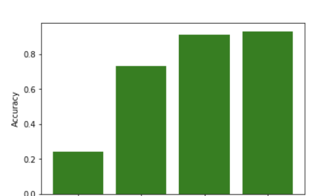
[Non-rotated spherical MNIST classification using $\lim_{J\rightarrow\infty}S_{J}^{L}f$ for different network depths $L$. Depth $L=3$ obtains $93$% classification accuracy.] [Spherical MNIST classification with not rotated (NR) and rotated (R) datasets. Note that Cohen et al. (2018); Kondor et al. (2018a); Jiang et al. (2019) utilize fully learned filters specifically designed for the sphere.] Model NR R S2CNN (Cohen et al., 2018) $0.96$ $0.95$ FFS2CNN (Kondor et al., 2018a) $0.96$ $0.97$ Method from Jiang et al. (2019) $0.99$ N/A Haar wavelet scattering (Chen et al., 2014) $0.90$ N/A Geometric scattering, $J=-2$, $L=2$ $0.95$ $0.95$

Figure 3: Spherical MNIST classificaion results.

5.2 FAUST

The FAUST dataset (Bogo et al., 2014) contains ten poses from ten people resulting in a total of 100 manifolds represented by triangle meshes. We first consider the problem of classifying poses. This task requires globally invariant features, and thus we compute the globally invariant geometric wavelet scattering transform $\overline{S}^{L}f$ of Section 3.3. Following the common practice of other geometric deep learning methods (see, e.g., Litany et al., 2017; Lim et al., 2019), we use 352 SHOT features (Tombari et al., 2010; Prakhya et al., 2015) as initial node features $f$. We used 5-fold cross validation for the classification tests with nested cross validation to tune the hyper-parameters of the RBF kernel SVM, as well as the network depth $L$. We remark that tuning the network depth of the geometric scattering transform is relatively simple as compared to fully learned geometric deep networks, since the filters are predefined geometric wavelets. This is particularly important for smaller data sets such as FAUST where there is a limited amount of training data. As indicated in Table 3, we achieve 95% overall accuracy using the geometric scattering features, compared to 92% accuracy achieved using only the integrals of SHOT features (i.e., restricting to $L=0$). We note that Masci et al. (2015) also considered pose classification, but the authors used a different training/test split (50% for training and 50% for test in a leave-one-out fashion), so our results are not directly comparable.

As a second task, we attempt to classify the people. This task is even more challenging than classifying the poses since some of the people are very similar to each other. We again performed 5-fold cross-validation, with each fold containing two poses from each person to ensure the folds are evenly distributed. As shown in Table 1, we achieved 76% accuracy on this task compared to the 61% accuracy using only integrals of SHOT features. In order to further emphasize the difference between the discretized geometric scattering transform and the graph scattering transform, we also attempted this task using the graph scattering transform derived from the graph Laplacian of the manifold mesh, applied to the SHOT features of each manifold. For this approach, which is representative of the aforementioned graph scattering papers, we obtained 58% accuracy. This result is similar to the 61% accuracy obtained by the baseline SHOT feature approach and empirically indicates the importance of encoding geometric information into the scattering transform for manifold-based tasks. More details regarding both tasks are in Appendix K.

Table 1: Manifold classification on FAUST dataset with two tasks.

Task/Model SHOT only Geometric scattering Pose classification $0.92$ $0.95$ Person classification $0.61$ $0.76$

6 Conclusion

We have constructed a geometric version of the scattering transform on a large class of Riemannian manifolds and shown this transform is non-expansive, invariant to isometries, and stable to diffeomorphisms. Our construction uses the spectral decomposition of the Laplace-Beltrami operator to construct a class of spectral filtering operators that generalize convolution on Euclidean space. While our numerical examples demonstrate geometric scattering on two-dimensional manifolds, our theory remains valid for manifolds of any dimension $d,$ and therefore can be naturally extended and applied to higher-dimensional manifolds in future work. Finally, our construction provides a mathematical framework that enables future analysis and understanding of geometric deep learning.

This research was partially funded by: grant P42 ES004911, through the National Institute of Environmental Health Sciences of the NIH, supporting F.G.; IVADO (l’institut de valorisation des données) [G.W.]; the Alfred P. Sloan Fellowship (grant FG-2016-6607), the DARPA Young Faculty Award (grant D16AP00117), the NSF CAREER award (grant 1845856), and NSF grant 1620216 [M.H.]; NIH grant R01GM135929 [M.H. & G.W]. The content provided here is solely the responsibility of the authors and does not necessarily represent the official views of the funding agencies.

Appendix A Proof of Theorem 2.1

*

We will prove a result that generalizes Theorem 2.1 to isometries between different manifolds. This more general result will be needed to prove Theorem 3.4.

Before stating our more general result, we introduce some notation. Let $\mathcal{M}$ and $\mathcal{M}^{\prime}$ be smooth compact connected Riemannian manifolds without boundary, and let $\zeta:\mathcal{M}\rightarrow\mathcal{M}^{\prime}$ be an isometry. Since $\mathcal{M}$ and $\mathcal{M}^{\prime}$ are and isometric, their Laplace Beltrami operators $\Delta$ and $\Delta^{\prime}$ have the same eigenvalues, and we enumerate the eigenvalues of $-\Delta$ (and also of $-\Delta^{\prime}$) in increasing order (repeating those with multiplicity greater than one) as $0=\lambda_{0}<\lambda_{1}\leq\lambda_{2}\leq\ldots.$ Recall that if $h\in\mathbf{L}^{2}(\mathcal{M})$ is a spectral filter, then by definition, there exists a function $H:[0,\infty)\rightarrow\mathbb{R}$ such that

$$H(\lambda_{k})\coloneqq\widehat{h}(k),\>\text{for all }k\geq 0\,,$$

and that

$$K_{h}(x,y)=\sum_{k\geq 0}\widehat{h}(k)\varphi_{k}(x)\overline{\varphi_{k}(y)}=\sum_{k\geq 0}H(\lambda_{k})\varphi_{k}(x)\overline{\varphi_{k}(y)}\,.$$

Therefore, we may define an operator $T_{h}^{\prime},$ on $\mathbf{L}^{2}(\mathcal{M}^{\prime}),$ which we consider the analogue of $T_{h},$ as integration against the kernel

$$K^{\prime}_{h}(x,y)\coloneqq\sum_{k\geq 0}H(\lambda_{k})\varphi_{k}^{\prime}(x)\overline{\varphi_{k}^{\prime}(y)}\,,$$

where $\varphi^{\prime}_{0},\varphi^{\prime}_{1},\ldots,$ is an orthonormal basis of eigenfunction on $\mathbf{L}^{2}(\mathcal{M}^{\prime})$ with $-\Delta^{\prime}\varphi_{k}^{\prime}=\lambda_{k}\varphi_{k}^{\prime}.$ With this notation, we may now state a generalized version of Theorem 2.1 (to recover Theorem 2.1, we set $\mathcal{M}^{\prime}=\mathcal{M}$).

Theorem A.1

Let $\zeta:\mathcal{M}\rightarrow\mathcal{M}^{\prime}$ be an isometry. Then for every spectral filter $h$ and every $f\in\mathbf{L}^{2}(\mathcal{M}),$

$$T_{h}^{\prime}V_{\zeta}(f)=V_{\zeta}T_{h}f\,.$$

Proof A.1.

For $\lambda\in\Lambda,$ let $\pi_{\lambda}$ be the operator which projects a function $f\in\mathbf{L}^{2}(\mathcal{M})$ onto the corresponding eigenspace $E_{\lambda},$ and let $\pi_{\lambda}^{\prime}$ be the analogous operator defined on $\mathbf{L}^{2}(\mathcal{M}^{\prime}).$ Since $\{\varphi_{k}\}_{\lambda_{k}=\lambda}$ forms an orthonormal basis for $E_{\lambda}$, we may write write $\pi_{\lambda}$ as integration against the kernel $K^{(\lambda)}(x,y)$ defined in (3), i.e.,

$$\pi_{\lambda}f(x)=\int_{\mathcal{M}}K^{(\lambda)}(x,y)f(y)dy\,.$$

Recalling from (4) that

$$K_{h}(x,y)=\sum_{\lambda\in\Lambda}H(\lambda)K^{(\lambda)}(x,y)\,,$$

we see that

$$T_{h}f=\sum_{\lambda\in\Lambda}H(\lambda)\pi_{\lambda}f\,,$$

and likewise,

$$T_{h}^{\prime}f=\sum_{\lambda\in\Lambda}H(\lambda)\pi^{\prime}_{\lambda}f\,.$$

Therefore, by the linearity of $V_{\zeta},$ it suffices to show that

$$\pi^{\prime}_{\lambda}V_{\zeta}f=V_{\zeta}\pi_{\lambda}f$$

for all $f\in\mathbf{L}^{2}(\mathcal{M})$ and all $\lambda\in\Lambda.$ Let $f\in\mathbf{L}^{2}(\mathcal{M})$ and write

$$f=f_{1}+f_{2}\,,$$

where $f_{1}\in E_{\lambda},f_{2}\in E_{\lambda}^{\perp}.$ Since $\zeta$ is an isometry, we have $V_{\zeta}f_{1}\in E_{\lambda}^{\prime}$ and $V_{\zeta}f_{2}\in\left(E_{\lambda}^{\prime}\right)^{\perp}.$ Therefore,

$$\pi_{\lambda}^{\prime}V_{\zeta}f=\pi_{\lambda}^{\prime}V_{\zeta}f_{1}+\pi_{\lambda}^{\prime}V_{\zeta}f_{2}=V_{\zeta}f_{1}=V_{\zeta}\pi_{\lambda}f$$

as desired.

Appendix B Proof of Proposition 2.2

*

Proof B.1.

Analogously to Parseval’s theorem, it follows from the Fourier inversion formula (1) and the fact that $\{\varphi_{k}\}_{k\geq 0}$ is an orthonormal basis, that

$$\|f\|_{2}^{2}=\sum_{k\geq 0}|\widehat{f}(k)|^{2}\,.$$

Similarly, it follows from (2) that

$$\|f\ast h_{\gamma}\|_{2}^{2}=\sum_{k\geq 0}|\widehat{h_{\gamma}}(k)|^{2}|\widehat{f}(k)|^{2}\,.$$

Therefore, using the Littlewood Paley condition (5), we see

$$\|\mathcal{H}f\|_{2,2}^{2} =\sum_{\gamma\in\Gamma}\|f\ast h_{\gamma}\|_{2}^{2}$$

$$=\sum_{\gamma\in\Gamma}\sum_{k\geq 0}|\widehat{h_{\gamma}}(k)|^{2}|\widehat{f}(k)|^{2}$$

$$=\sum_{k\geq 0}|\widehat{f}(k)|^{2}\sum_{\gamma\in\Gamma}|\widehat{h_{\gamma}}(k)|^{2}$$

$$=\sum_{k\geq 0}|\widehat{f}(k)|^{2}$$

$$=\|f\|^{2}_{2}\,.$$

Appendix C Proof of Proposition 2.3

*

Proof C.1.

We will show that the frame $\{\phi_{J}\,,\,\psi_{j}:j\leq J\}$ satisfies the Littlewood Paley condition (5), i.e. that

$$|\widehat{\phi}_{J}(k)|^{2}+\sum_{j\leq J}|\widehat{\psi}_{j}(k)|^{2}=1,\quad\forall\,k\geq 0\,.$$

The result will then follow from Proposition 2.2. Recall that $\phi_{J}$ is defined by $\widehat{\phi}_{J}(k)=G\left(2^{J}\lambda_{k}\right)$ for some non-negative, non-increasing function $G$ such that $G(0)=1$. Therefore, from (6), we see that that

$$|\widehat{\psi}_{j}(k)|^{2}=|\widehat{\phi}_{j-1}(k)|^{2}-|\widehat{\phi}_{j}(k)|^{2}=|G(2^{j-1}\lambda_{k})|^{2}-|G(2^{j}\lambda_{k})|^{2},$$

and so,

$$|\widehat{\phi}_{J}(k)|^{2}+\sum_{j\leq J}|\widehat{\psi}_{j}(k)|^{2} =\left|G\left(2^{J}\lambda_{k}\right)\right|^{2}+\sum_{j\leq J}\left[\left|G\left(2^{j-1}\lambda_{k}\right)|^{2}-|G\left(2^{j}\lambda_{k}\right)\right|^{2}\right]$$

$$=\lim_{j\rightarrow-\infty}|G\left(2^{j}\lambda_{k}\right)|^{2}$$

$$=|G(0)|^{2}=1,\quad\forall\,k\geq 0\,.$$

Appendix D The Proof of Theorem 3.3

*

The proof of Theorem 3.3 relies on the following two lemmas.

Lemma 1.

There exists a constant $C(\mathcal{M})>0$ such that for every spectral filter $h$ and for every $\zeta\in\mathrm{Diff}(\mathcal{M})$,

$$\|T_{h}f-V_{\zeta}T_{h}f\|_{2}\leq C(\mathcal{M})\left(\sum_{k\geq 0}\widehat{h}(k)\lambda_{k}^{d/2}\right)\|\zeta\|_{\infty}\|f\|_{2}\,,\quad\forall\,f\in\mathbf{L}^{2}(\mathcal{M})\,.$$

Moreover, if $|\widehat{h}(k)|\leq e^{-2^{J}\lambda_{k}},$ then there exists a constant $C(\mathcal{M})>0$ such that for any $\zeta\in\mathrm{Diff}(\mathcal{M})$,

$$\|T_{h}f-V_{\zeta}T_{h}f\|_{2}\leq C(\mathcal{M})2^{-dJ}\|\zeta\|_{\infty}\|f\|_{2}\,,\quad\forall\,f\in\mathbf{L}^{2}(\mathcal{M})\,.$$

Lemma 2.

For any $f\in\mathbf{L}^{2}(\mathcal{M})$,

$$\|U_{J}^{L}f\|_{2,2}\leq(L+1)^{1/2}\|f\|_{2}\,.$$

Proof D.1 (The Proof of Theorem 3.3).

Theorem 2.1 proves that spectral filter convolution operators commute with isometries. Since the absolute value operator does as well, it follows that $V_{\zeta}S_{J}^{L}=S_{J}^{L}V_{\zeta},$ and therefore

$$\|S_{J}^{L}f-S_{J}^{L}V_{\zeta}f\|_{2,2}=\|S_{J}^{L}f-V_{\zeta}S_{J}^{L}f\|_{2,2}\,.$$

Since $S_{J}^{L}=A_{J}U_{J}^{L}$, we see that

$$\|S_{J}^{L}f-V_{\zeta}S_{J}^{L}f\|_{2,2} =\|A_{J}U_{J}^{L}f-V_{\zeta}A_{J}U_{J}^{L}f\|_{2,2}\leq\|A_{J}-V_{\zeta}A_{J}\|\|U_{J}^{L}f\|_{2,2}\,.$$ (23)

Since $A_{J}=T_{\phi_{J}}$ and $|\widehat{\phi_{J}}(k)|\leq e^{-2^{J}\lambda_{k}}$, Lemma 1 shows that

$$\|A_{J}-V_{\zeta}A_{J}\|\leq C(\mathcal{M})2^{-Jd}\|\zeta\|_{\infty}\,.$$

Equation (12) follows from Lemma 2, and (11) follows by letting $L$ increase to infinity in (23). Therefore, the proof is complete pending the proof of Lemmas 1 and 2.

Proof D.2 (The Proof of Lemma 2).

Let

$$\widetilde{U}_{J}^{L}f \coloneqq\{U_{J}^{L}[j_{1},\ldots,j_{L}]f:\,j_{i}\leq J\enspace\forall\,1\leq i\leq L\}$$

$$=\{|||f\ast\psi_{j_{1}}|\ast\psi_{j_{2}}|\ast\cdots\ast\psi_{j_{L}}|:\,j_{i}\leq J\enspace\forall\,1\leq i\leq L\}\,.$$

Then, by construction,

$$\|U_{J}^{L}f\|_{2,2}^{2}=\sum_{\ell=0}^{L}\|\widetilde{U}_{J}^{\ell}f\|_{2,2}^{2}$$ (24)

where we adopt the convention that $\widetilde{U}^{0}_{J}f=\{f\}.$ Since the wavelet transform and the absolute value operator are both non-expansive, it follows that $\widetilde{U}_{J}^{1}$ is non-expansive as well. Therefore, since $\widetilde{U}_{J}^{L}=\widetilde{U}_{J}^{1}\widetilde{U}_{J}^{L-1},$ we see

$$\|\widetilde{U}_{J}^{L}f\|_{2,2}\leq\|\widetilde{U}_{J}^{L-1}f\|_{2,2}\leq\ldots\leq\|\widetilde{U}_{J}^{1}f\|_{2,2}\leq\|f\|_{2}\,.$$

Therefore, (24) implies

$$\|U_{J}^{L}\|_{2,2}^{2}=\sum_{\ell=0}^{L}\|\widetilde{U}_{J}^{\ell}\|_{2,2}^{2}\leq(L+1)\|f\|_{2}^{2}$$

as desired.

In order to prove Lemma 1, we will first prove the following lemma.

Lemma 3.

For $\lambda\in\Lambda,$ let $K^{(\lambda)}$ be the kernel defined as in $\eqref{eqn: Klambda definition},$ and let $m(\lambda)$ be the multiplicity of $\lambda$. Then, there exists a constant $C(\mathcal{M})>0$ such that

$$\left\|\nabla K^{(\lambda)}\right\|_{\infty}\leq C(\mathcal{M})m(\lambda)\lambda^{d/2}\,,\quad\forall\,\lambda\in\Lambda\,.$$ (25)

As a consequence, if $K_{h}$ is a spectral kernel, then

$$\|\nabla K_{h}\|_{\infty}\leq C(\mathcal{M})\sum_{\lambda\in\Lambda}H(\lambda)m(\lambda)\lambda^{d/2}=C(\mathcal{M})\sum_{k\geq 0}\widehat{h}(k)\lambda_{k}^{d/2}\,.$$ (26)

Furthermore, if $\mathcal{M}$ is homogeneous, i.e., if for all $x,y\in\mathcal{M},$ there exists an isometry mapping $x$ to $y,$ then

$$\left\|\nabla K^{(\lambda)}\right\|_{\infty}\leq C(\mathcal{M})m(\lambda)\lambda^{(d+1)/4}$$ (27)

and thus,

$$\|\nabla K_{h}\|_{\infty}\leq C(\mathcal{M})\sum_{\lambda\in\Lambda}H(\lambda)m(\lambda)\lambda^{(d+1)/4}=C(\mathcal{M})\sum_{k\in\mathbb{N}}\widehat{h}(k)\lambda_{k}^{(d+1)/4}\,.$$ (28)

Proof D.3.

For any $k$ such that $\lambda_{k}=\lambda,$ it is a consequence of Hörmander’s local Weyl law (Hörmander (1968); see also Shi and Xu (2010)) that

$$\|\varphi_{k}\|_{\infty} \leq C(\mathcal{M})\lambda^{(d-1)/4}\,.$$

Theorem 1 of Shi and Xu (2010) shows that

$$\|\nabla\varphi_{k}\|_{\infty} \leq C(\mathcal{M})\sqrt{\lambda}\|\varphi_{k}\|_{\infty}\,.$$

Therefore,

$$\left|\nabla K^{(\lambda)}(x,y)\right|^{2} =\left|\sum_{k:\lambda_{k}=\lambda}\nabla\varphi_{k}(x)\overline{\varphi}_{k}(y)\right|^{2}$$

$$\leq\left(\sum_{k:\lambda_{k}=\lambda}|\nabla\varphi_{k}(x)|^{2}\right)\left(\sum_{k:\lambda_{k}=\lambda}|\varphi_{k}(y)|^{2}\right)$$

$$\leq C(\mathcal{M})m(\lambda)\lambda^{(d-1)/2}\sum_{k:\lambda_{k}=\lambda}|\nabla\varphi_{k}(x)|^{2}$$

$$\leq C(\mathcal{M})m(\lambda)\lambda^{(d+1)/2}\sum_{k:\lambda_{k}=\lambda}\|\varphi_{k}\|_{\infty}^{2}$$

$$\leq C(\mathcal{M})m(\lambda)^{2}\lambda^{d}\,.$$

This implies (25). Now, if we assume that $\mathcal{M}$ is homogeneous, then Theorem 3.2 of Evariste (1975) shows that

$$\sum_{k:\lambda_{k}=\lambda}|\varphi_{k}(y)|^{2}=C(\mathcal{M})m(\lambda)\,.$$

Substituting this into the above string of inequalities yields (27). Equations (26) and (28) follow by recalling from (4) that

$$K_{h}(x,y)=\sum_{\lambda\in\Lambda}H(\lambda)K^{(\lambda)}(x,y)\,,$$

and applying the triangle inequality.

Now we may prove Lemma 1.

Proof D.4 (The Proof of Lemma 1).

Let $K_{h}$ be the kernel of $T_{h}$. Then by the Cauchy-Schwartz inequality and the fact that $V_{\zeta}f(x)=f\left(\zeta^{-1}(x)\right),$

$$|T_{h}f(x)-V_{\zeta}T_{h}f(x)| =\left|\int_{\mathcal{M}}\left[K_{h}(x,y)-K_{h}\left(\zeta^{-1}(x),y\right)\right]f(y)\,dy\right|$$

$$\leq\|f\|_{2}\left(\int_{\mathcal{M}}\left|K_{h}(x,y)-K_{h}\left(\zeta^{-1}(x),y\right)\right|^{2}\,dy\right)^{1/2}$$

$$\leq\|f\|_{2}\|\nabla K_{h}\|_{\infty}\left(\int_{\mathcal{M}}\left|r\left(x,\zeta^{-1}(x)\right)\right|^{2}\,dy\right)^{1/2}$$

$$\leq\|f\|_{2}\sqrt{\mathrm{vol}(\mathcal{M})}\|\nabla K_{h}\|_{\infty}\|\zeta\|_{\infty}\,.$$

It follows that

$$\|T_{h}f-V_{\zeta}T_{h}f\|_{2}\leq\mathrm{vol}(\mathcal{M})\|\nabla K_{h}\|_{\infty}\|\zeta\|_{\infty}\,.$$ (29)

Lemma 3 shows

$$\|\nabla K_{h}\|_{\infty}\leq C(\mathcal{M})\sum_{k\geq 0}\widehat{h}(k)\lambda_{k}^{d/2}\,,$$

and therefore

$$\|T_{h}f-V_{\zeta}T_{h}f\|_{2}\leq C(\mathcal{M})\left(\sum_{k\geq 0}\widehat{h}(k)\lambda_{k}^{d/2}\right)\|\zeta\|_{\infty}\,.$$

Now suppose that $G(\lambda)\leq e^{-\lambda}$. Theorem 2.4 of Bérard et al. (1994) proves that for any $x\in\mathcal{M}$, $\alpha\geq 0$, and $t>0$,

$$\sum_{k\geq 1}\lambda_{k}^{\alpha}e^{-t\lambda_{k}}|\varphi_{k}(x)|^{2}\leq C(\mathcal{M})(\alpha+1)t^{-(d+2\alpha)/2}\,.$$ (30)

Integrating both sides over $\mathcal{M}$ yields:

$$\sum_{k\geq 1}\lambda_{k}^{\alpha}e^{-t\lambda_{k}}\leq C(\mathcal{M})(\alpha+1)t^{-(d+2\alpha)/2}\,.$$ (31)

Using the assumption that that $|\widehat{h}(k)|\leq e^{-2^{J}\lambda_{k}},$ (29) and (31) with $\alpha=d/2$ and $t=2^{J},$ we see

$$\|T_{h}f-V_{\zeta}T_{h}f\|_{2} \leq C(\mathcal{M})\left(\sum_{k\geq 1}\lambda_{k}^{d/2}e^{-2^{J}\lambda_{k}}\right)\|\zeta\|_{\infty}$$

$$\leq C(\mathcal{M})2^{-dJ}\|\zeta\|_{\infty}\,.$$

Appendix E The Proof of Theorem 3.3

*

Proof E.1.

Let $p=\emptyset$ or $p=(j_{1},\ldots,j_{m})$ denote a scattering path. Using (13), implies

$$\lim_{J\rightarrow\infty}\left\|\frac{|S_{J}[p]f|}{\mathrm{vol}(\mathcal{M})^{-1/2}}-\overline{S}[p]f\right\|_{2}=0,$$

and therefore

$$\lim_{J\rightarrow\infty}\left\|\frac{|S_{J}[p]f|}{\mathrm{vol}(\mathcal{M})^{-1/2}}\right\|_{2}={\mathrm{vol}(\mathcal{M})^{1/2}}\overline{S}[p]f.$$

Thus, using Fatou’s lemma, we have

$$\|\overline{S}f\|_{2}^{2} =\sum_{p}|\overline{S}[p]f|^{2}$$

$$=\frac{1}{\mathrm{vol}(\mathcal{M})}\sum_{p}\lim_{J\rightarrow\infty}\left\|\frac{|S_{J}[p]f|}{\mathrm{vol}(\mathcal{M})^{-1/2}}\right\|_{2}^{2}$$

$$\leq\liminf_{J\rightarrow\infty}\sum_{p}\left\||S_{J}[p]f|\right\|_{2}^{2}$$

$$\leq\|f\|_{2},$$

where in the last line we applied Proposition 3.1.

Appendix F The Proof of Proposition 3.4

*

Proof F.1.

Letting $p=\emptyset$ or $p=(j_{1},\ldots,j_{m})$ denote a scattering path, we see that we need to prove $\overline{S}[p]f=\overline{S}^{\prime}V_{\zeta}f[p]$ for all $p\in\mathcal{P}$. If $p=\emptyset$ then $\overline{S}f(\emptyset)=\|f\|_{\mathbf{L}^{1}(\mathcal{M})}=\|V_{\zeta}f\|_{\mathbf{L}^{1}(\mathcal{M}^{\prime})}=\overline{S}^{\prime}V_{\zeta}f(\emptyset)$ since $\zeta$ is an isometry. Theorem A.1, stated in Appendix A, proves that $T_{h}^{\prime}V_{\zeta}f=V_{\zeta}T_{h}f$ for any spectral filter $h\in\mathbf{L}^{2}(\mathcal{M})$, where $T_{h}^{\prime}$ is the analogue of $T_{h}$ on $\mathbf{L}^{2}(\mathcal{M}^{\prime})$ (defined precisely in Appendix A). Since the modulus operator also commutes with isometries, it follows that $U^{\prime}[p]V_{\zeta}f=V_{\zeta}U[p]f$ for any $p\in\mathcal{P}.$ Thus, since $\zeta$ is an isometry,

$$\overline{S}^{\prime}V_{\zeta}f(p)=\|U^{\prime}[p]V_{\zeta}f\|_{\mathbf{L}^{1}(\mathcal{M}^{\prime})}=\|V_{\zeta}U[p]f\|_{\mathbf{L}^{1}(\mathcal{M}^{\prime})}=\|U[p]f\|_{\mathbf{L}^{1}(\mathcal{M})}=\overline{S}f(p)\,.$$

Appendix G The Proof of Theorem 3.4

*

Proof G.1.

As in the proof of Theorem 3.3, we observe that since spectral filter convolution operators and the absolute value operator both commute with isometries, it follows that $\left(S_{J}^{L}\right)^{\prime}V_{\zeta_{1}}=V_{\zeta_{1}}S_{J}^{L}.$ Therefore

$$\|S_{J}^{L}f-V_{\zeta_{2}^{-1}}\left(S_{J}^{L}\right)^{\prime}V_{\zeta_{1}}f\|_{2,2}=\|S_{J}^{L}f-V_{\zeta_{2}^{-1}}V_{\zeta_{1}}S_{J}^{L}f\|_{2,2}=\|S_{J}^{L}f-V_{\zeta_{2}^{-1}\circ\zeta_{1}}S_{J}^{L}f\|_{2,2}\,.$$

Equation (15) now follows by applying (12). The proof of (14) is similar and follows by applying (11).

Appendix H The Proof of Theorems 4.1 and 4.1

*

* In order to prove Theorem 4.1, we will need the following lemma.

Lemma 1.

If $f\in\mathbf{L}^{2}(\mathcal{M})$ is $\lambda$-bandlimited, i.e., $\langle f,\varphi_{k}\rangle=0$ whenever $\lambda_{k}>\lambda,$ then there exists a constant $C(\mathcal{M})<\infty$ such that

$$\|f-V_{\zeta}f\|_{2}\leq C(\mathcal{M})\lambda^{d}\|\zeta\|_{\infty}\|f\|_{2}$$

for all $\zeta\in\mathrm{Diff}(\mathcal{M})$.

Proof H.1.

As in the proof of Theorem A.1, let $\Lambda$ denote the set of unique eigenvalues of $-\Delta,$ and let $\pi_{\lambda}$ be the operator that projects a function $f\in\mathbf{L}^{2}(\mathcal{M})$ onto the eigenspace $E_{\lambda}.$ Let

$$P_{\lambda}\coloneqq\sum_{\tilde{\lambda}\leq\lambda}\pi_{\tilde{\lambda}}\,,$$

be the operator which projects a function $f\in\mathbf{L}^{2}(\mathcal{M})$ onto all eigenspaces with eigenvalues less than or equal to $\lambda.$ Note that $P_{\lambda}$ can be written as integration against the kernel

$$K(x,y)=\sum_{\lambda_{k}\leq\lambda}\varphi_{k}(x)\overline{\varphi}_{k}(y)=\sum_{\tilde{\lambda}\leq\lambda}K^{(\lambda)}(x,y)\,,$$

where $K^{(\lambda)}$ is defined as in (3). If $f$ is any $\lambda$-bandlimited function in $\mathbf{L}^{2}(\mathcal{M})$, then $P_{\lambda}f=f,$ and so similarly to the proof of Lemma 1, we see that

$$|f(x)-V_{\zeta}f(x)| =|P_{\lambda}f(x)-V_{\zeta}P_{\lambda}f(x)|$$

$$=\left|\int_{\mathcal{M}}K(x,y)f(y)dy-\int_{\mathcal{M}}K\left(\zeta^{-1}(x),y\right)f(y)dy\right|$$

$$\leq\|f\|_{2}\left(\int_{\mathcal{M}}\left|K(x,y)-K\left(\zeta^{-1}(x),y\right)\right|^{2}dy\right)^{1/2}$$

$$\leq\|f\|_{2}\|\zeta\|_{\infty}\sqrt{\mathrm{vol}(\mathcal{M})}\|\nabla K\|_{\infty}\,,$$

which implies

$$\|f-V_{\zeta}f\|_{2}\leq\mathrm{vol}(\mathcal{M})\|\nabla K\|_{\infty}\|\zeta\|_{\infty}\|f\|_{2}\,.$$

Lemma 3 shows that for all $\tilde{\lambda}$

$$\left\|\nabla K^{(\tilde{\lambda})}\right\|_{\infty}\leq C(\mathcal{M})m(\tilde{\lambda})\tilde{\lambda}^{d/2}\,.$$

Therefore,

$$\|\nabla K\|_{\infty}\leq C(\mathcal{M})\sum_{\lambda_{k}\leq\lambda}\left(\lambda_{k}\right)^{d/2}\leq C(\mathcal{M})N(\lambda)\lambda^{d/2}\,,$$

where $N(\lambda)$ is the number of eigenvalues less than or equal to $\lambda.$ Weyl’s law (see for example Ivrii (2016)) implies that

$$N(\lambda)\leq C(\mathcal{M})\lambda^{d/2}\,,$$

and so

$$\|\nabla K\|_{\infty}\leq C(\mathcal{M})\lambda^{d}\,.$$

Proof H.2 (The Proof of Theorem 4.1).

Let $\zeta=\zeta_{2}\circ\zeta_{1}$ be a factorization of $\zeta$ such that $\zeta_{1}$ is an isometry and $\zeta_{2}$ is a diffeomorphism. Then since $V_{\zeta}f=f\circ\zeta^{-1},$ we see that $V_{\zeta}=V_{\zeta_{2}}V_{\zeta_{1}}.$ Therefore, for all $\lambda$-bandlimited functions $f$

$$\|S_{J}^{L}f-S_{J}^{L}V_{\zeta}f\|_{2,2}\leq\|S_{J}^{L}f-S_{J}^{L}V_{\zeta_{1}}f\|_{2,2}+\|S_{J}^{L}V_{\zeta_{1}}f-S_{J}^{L}V_{\zeta_{2}}V_{\zeta_{1}}f\|_{2,2}\,.$$

By (12), we have that

$$\|S_{J}^{L}f-S_{J}^{L}V_{\zeta_{1}}f\|_{2,2}\leq C(\mathcal{M})2^{-Jd}\|\zeta_{1}\|_{\infty}(L+1)^{1/2}\|f\|_{2}\,,$$

and by Proposition 3.1 and Lemma 1 we see

$$\|S_{J}^{L}V_{\zeta_{1}}f-S_{J}^{L}V_{\zeta_{2}}V_{\zeta_{1}}f\|_{2,2}\leq\|V_{\zeta_{1}}f-V_{\zeta_{2}}V_{\zeta_{1}}f\|_{2}\leq C(\mathcal{M})\lambda^{d}\|\zeta_{2}\|_{\infty}\|V_{\zeta_{1}}f\|_{2}\,.$$

Since $\zeta_{1}$ is an isometry, we observe that $\|V_{\zeta_{1}}f\|_{2}=\|f\|_{2}.$ Combining this with the two inequalities above completes the proof of (17). The proof of (16) is similar, but uses (11) instead of (12).

Proof H.3 (The Proof of Theorem 4.1).

Repeating the proof of Proposition 3.4 we see that

$$\|\overline{S}f-\overline{S}V_{\zeta}f\|_{2,2}\leq\lim_{J\rightarrow\infty}\|S_{J}f-S_{J}V_{\zeta}f\|_{2,2}.$$

Therefore, the result follows from Theorem 4.1 by taking $J\rightarrow\infty$ on the right hand side of (16).

Appendix I The Proof of Theorem 4.2

*

In order to prove Theorem 4.2, we will need the an auxiliary result, which provides a commutator estimate for operators with radial kernels. We will say that a kernel operator

$$Tf(x)=\int_{\mathcal{M}}K(x,y)f(y)\,dy$$

is radial if

$$K(x,y)=\kappa(r(x,y))$$

for some $\kappa:[0,\infty)\rightarrow\mathbb{C}.$ The following theorem establishes a commutator estimate for operators with radial kernels.

Theorem 1.

Let $T$ be a kernel integral operator with a radial kernel $K(x,y)=\kappa(r(x,y))$ for some $\kappa\in\mathbf{C}^{1}(\mathbb{R})$. Then there exists constants $C_{1}(\mathcal{M},K)$ and $C_{2}(\mathcal{M},K)$ such that

$$\|[T,V_{\zeta}]f\|_{2}\leq\|f\|_{2}\left[C_{1}(\mathcal{M},K)A_{1}(\zeta)+C_{2}(\mathcal{M},K)A_{2}(\zeta)\right]\,.$$

Here $A_{1}(\zeta)$ and $A_{2}(\zeta)$ are defined as in (21) and (22) respectively,

$$C_{1}(\mathcal{M},K)=\|\nabla K\|_{\infty}\mathrm{diam}(\mathcal{M})\mathrm{vol}(\mathcal{M})\,,$$

and

$$C_{2}(\mathcal{M},K)=\|K\|_{\mathbf{L}^{2}(\mathcal{M}\times\mathcal{M})}\,.$$

Proof I.1.

We first compute

$$|[T,V_{\zeta}]f(x)| =\left|\int_{\mathcal{M}}K(x,y)f(\zeta^{-1}(y))\,dy-\int_{\mathcal{M}}K(\zeta^{-1}(x),y)f(y)\,dy\right|$$

$$=\left|\int_{\mathcal{M}}K(x,\zeta(y))f(y)|\det[D\zeta(y)]|\,dy-\int_{\mathcal{M}}K(\zeta^{-1}(x),y)f(y)\,dy\right|$$

$$=\left|\int_{\mathcal{M}}f(y)\left[K(x,\zeta(y))|\det[D\zeta(y)]|-K(\zeta^{-1}(x),y)\right]\,dy\right|$$

$$\leq\left|\int_{\mathcal{M}}f(y)\left[K(x,\zeta(y))[|\det[D\zeta(y)]|-1\right]\,dy\right|+\left|\int_{\mathcal{M}}f(y)\left[K(x,\zeta(y))-K(\zeta^{-1}(x),y)\right]\,dy\right|$$

$$\leq\||\det[D\zeta(y)]|-1\|_{\infty}\left|\int_{\mathcal{M}}f(y)K(x,\zeta(y))\,dy\right|+\left|\int_{\mathcal{M}}f(y)\left[K(x,\zeta(y))-K(\zeta^{-1}(x),y)\right]\,dy\right|.$$

Therefore, by the Cauchy-Schwartz inequality,

$$\|[T,V_{\zeta}]f\|_{2}\leq\|f\|_{2}\Bigg{[} \||\det[D\zeta(y)]|-1\|_{\infty}\bigg{(}\int_{\mathcal{M}}\int_{\mathcal{M}}\left|K(x,\zeta(y))\right|^{2}\,dy\,dx\bigg{)}^{\frac{1}{2}}$$

$$+\bigg{(}\int_{\mathcal{M}}\int_{\mathcal{M}}\left|K(x,\zeta(y))-K(\zeta^{-1}(x),y)\right|^{2}\,dy\,dx\bigg{)}^{\frac{1}{2}}\Bigg{]}\,.$$

We may bound the first integral by observing

$$\int_{\mathcal{M}}\int_{\mathcal{M}}\left|K(x,\zeta(y))\right|^{2}\,dy\,dx\leq\|\det[D\zeta^{-1}(y)]\|^{2}_{\infty}\int_{\mathcal{M}}\int_{\mathcal{M}}\left|K(x,y)\right|^{2}\,dy\,dx\,.$$

To bound the second integral observe, that by the mean value theorem and the assumption that $K$ is radial, we have

$$\int_{\mathcal{M}}\int_{\mathcal{M}}|K(x,\zeta(y)) -K(\zeta^{-1}(x),y)|^{2}\,dy\,dx$$

$$=\int_{\mathcal{M}}\int_{\mathcal{M}}\left|\kappa(r(x,\zeta(y)))-\kappa(r(\zeta^{-1}(x),y))\right|^{2}\,dy\,dx$$

$$\leq\|\kappa^{\prime}\|_{\infty}^{2}\int_{\mathcal{M}}\int_{\mathcal{M}}\left|r(x,\zeta(y))-r(\zeta^{-1}(x),y)\right|^{2}\,dy\,dx$$

$$\leq\left[\|\kappa^{\prime}\|_{\infty}A_{1}(\zeta)\right]^{2}\int_{\mathcal{M}}\int_{\mathcal{M}}\left|r(x,\zeta(y))\right|^{2}\,dy\,dx$$

$$\leq\left[\|\kappa^{\prime}\|_{\infty}A_{1}(\zeta)\mathrm{diam}(\mathcal{M})\mathrm{vol}(\mathcal{M})\right]^{2}.$$

Lastly, since $K(x,y)=\kappa(r(x,y)),$ we see that

$$\|\nabla K\|_{\infty}=\|\kappa^{\prime}\|_{\infty}\,,$$

which completes the proof.

Proof I.2 (The Proof of Theorem 4.2).

We write $T=T_{h}$ and $K=K_{h}$. If $\mathcal{M}$ is two-point homogeneous and $r(x,y)=r(x^{\prime},y^{\prime}),$ then by the definition of two-point homogeneity there exists an isometry $\widetilde{\zeta}$ mapping $x\mapsto x^{\prime}$ and $y\mapsto y^{\prime}$. Therefore, we may use the proof of Theorem 2.1 to see that $K(x^{\prime},y^{\prime})=K(x,y)$. It follows that $K(x,y)$ is radial and so we may write $K(x,y)=\kappa(r(x,y))$ for some $\kappa\in\mathbf{C}^{1}$.

Applying Theorem 1, we see that

$$\|[T,V_{\zeta}]\|\leq C(\mathcal{M})\left[\|\nabla K\|_{\infty}A_{1}(\zeta)+\|K\|_{\mathbf{L}^{2}(\mathcal{M}\times\mathcal{M})}A_{2}(\zeta)\right].$$

Lemma 3 implies that

$$\|\nabla K\|_{\infty}\leq C(\mathcal{M})\sum_{k\in\mathbb{N}}H(\lambda_{k})\lambda_{k}^{(d+1)/4}\,,$$

and since $\{\varphi_{k}\}_{k=0}^{\infty}$ forms an orthonormal basis for $\mathbf{L}^{2}(\mathcal{M}),$ it can be checked that

$$\|K\|_{\mathbf{L}^{2}(\mathcal{M}\times\mathcal{M})}=\left(\sum_{k=0}^{\infty}|H(\lambda_{k})|^{2}\right)^{1/2}\,.$$

Therefore, the proof is complete since

$$A(\zeta)=\max\{A_{1}(\zeta),A_{2}(\zeta)\}$$

and

$$B(h)=\max\left\{\sum_{k\in\mathbb{N}}H(\lambda_{k})\lambda_{k}^{(d+1)/4},\left(\sum_{k\in\mathbb{N}}H(\lambda_{k})^{2}\right)^{\frac{1}{2}}\right\}\,.$$

Appendix J The Proof of Corollary 4.2

*

Proof J.1.

By the definition of $\widehat{\psi}_{j}$ and the assumption that $G(\lambda)\leq e^{-\lambda},$ we have that $\widehat{\psi}_{j}(0)=0$ and

$$|\widehat{\psi}_{j}(k)|\leq|\widehat{\phi}_{j-1}(k)|\leq e^{-2^{j-1}\lambda_{k}}$$

for $k\geq 1.$ Therefore, by Theorem 4.2,

$$\|[\Psi_{j},V_{\zeta}]\| \leq C(\mathcal{M})A(\zeta)B(\psi_{j})$$

where,

$$B(\psi_{j})=\max\left\{\sum_{k\geq 1}e^{-2^{j-1}\lambda_{k}}\lambda_{k}^{(d+1)/4},\left(\sum_{k\geq 1}e^{-2^{j}\lambda_{k}}\right)^{\frac{1}{2}}\right\}.$$

Equation (30) implies that

$$\sum_{k\geq 1}e^{-2^{j-1}\lambda_{k}}\lambda_{k}^{(d+1)/4}\leq C(\mathcal{M})2^{-(d+1/2)(j-1)}$$

and that

$$\sum_{k\geq 1}e^{-2^{j}\lambda_{k}}\leq C(\mathcal{M})2^{-dj/2}$$

thus completing the proof.

Appendix K Additional details of classification experiments

K.1 Spherical MNIST

For all spherical MNIST experiments, including those reported in Section 5.1, we used the following procedure. Since the digits six and nine are impossible to distinguish in spherical MNIST, we removed the digit six from the dataset. The mesh on the sphere consisted of 642 vertices, and to construct the wavelets on the sphere, all 642 eigenvalues and eigenfunctions of the approximate Laplace-Beltrami operator were used. For the range of scales we chose $-8\leq j\leq\min(0,J)$. Training and testing were conducted using the standard MNIST training set of 60,000 digits and the standard testing set of 10,000 digits, projected onto the sphere. The training set was randomly divided into five folds, of which four were used to train the RBF kernel SVM, taking as input the relevant geometric scattering representation of each spherically projected digit, and one was used to validate the hyper-parameters of the RBF kernel SVM (see Appendix K.3).

On both the non-rotated and randomly rotated spherical MNIST datasets, we calculated the geometric scattering coefficients $S_{J}^{L}f$ and downsampled the resulting scattering coefficient functions (e.g., $f\ast\phi_{J}(x)$ and $|f\ast\psi_{j}|\ast\phi_{J}(x)$). For $J\rightarrow\infty$ we selected one coefficient since they are all the same (recall (13)). With $J=0$, we selected 4 coefficients per function; with $J=-1$, we selected 16 coefficients; with $J=-2$, we selected 64 coefficients. The selected coefficients were determined by finding 4, 16, and 64 nearly equidistant points $x$ on the sphere. Classification results on the test set for a fixed network depth of $L=2$ and for the different values of $J$ are reported in Table 2 below. Figure 3 reports classification results for $J\rightarrow\infty$ and for $0\leq L\leq 3$.

Table 2: Geometric wavelet scattering classification results with with network depth $L=2$ for different $J$ on non-rotated and rotated spherical MNIST

$J$	NR	R
$J\rightarrow\infty$	$0.91$	$0.91$
$J=0$	$0.94$	$0.94$
$J=-1$	$0.95$	$0.95$
$J=-2$	$0.95$	$0.95$

K.2 FAUST

The FAUST dataset Bogo et al. (2014) consists of $100$ manifolds corresponding to ten distinct people in ten distinct poses. Each manifold is approximated by a mesh with $6890$ vertices. We used the $512$ smallest eigenvalues and corresponding eigenfunctions to construct the geometric wavelets. During cross validation, in addition to cross validating the SVM parameters (see Section K.3 below), we also cross validated the depth of the scattering network for $0\leq L\leq 2$. For the classification test, we performed $5$ fold cross validation with a training/validation/test split of 70%/10%/20% for both pose classification and person classification. The range of $j$ is chosen as $-11\leq j\leq 0$.

We report the frequency of each network depth $L$ selected during the hyperparameter cross validation stage. Since there are five test folds and eight validation folds, the depth is selected $40$ times per task. For pose classification, $L=0$ was selected $19$ times, $L=1$ was selected $11$ times, and $L=2$ was selected $10$ times. For person classification, $L=0$ was selected $5$ times, $L=1$ was selected $29$ times, and $L=2$ was selected $6$ times. The results indicate the importance of avoiding overfitting with needlessly deep scattering networks, while at the same time highlighting the task dependent nature of the network depth (compare as well to the MNIST results reported above and in the main text).

K.3 Parameters for RBF kernel SVM

We used RBF kernel SVM for all classification tasks and cross validated the hyperparameters. In the two FAUST classification tasks of Section 5.2, for the kernel width $\gamma$, we chose from $\{0.001,0.005,0.01,0.02,0.04\}$, while for the penalty $C$ we chose from $\{50,100,250,400,500\}$. For the spherical MNIST classification task of Section 5.1, for $\gamma$ we chose from $\{0.00001,0.0001,0.001\}$ and for $C$ we chose from $\{25,100,250,500\}$.

References

- Andén and Mallat (2011) Joakim Andén and Stéphane Mallat. Multiscale scattering for audio classification. In Proceedings of the ISMIR 2011 conference, pages 657–662, 2011.
- Andén and Mallat (2014) Joakim Andén and Stéphane Mallat. Deep scattering spectrum. IEEE Transactions on Signal Processing, 62(16):4114–4128, August 2014.
- Andén et al. (2019) Joakim Andén, Vincent Lostanlen, and Stéphane Mallat. Joint time-frequency scattering. IEEE Transactions on Signal Processing, 67(14):3704–3718, 2019.
- Bérard et al. (1994) Pierre Bérard, Gérard Besson, and Sylvain Gallot. Embedding Riemannian manifolds by their heat kernel. Geometric and Functional Analysis, 4(4):373–398, 1994.
- Bogo et al. (2014) Federica Bogo, Javier Romero, Matthew Loper, and Michael J. Black. FAUST: Dataset and evaluation for 3D mesh registration. In Proceedings of the IEEE Conference on Computer Vision and Pattern Recognition (CVPR), Piscataway, NJ, USA, 2014.
- Bronstein et al. (2017) Michael M. Bronstein, Joan Bruna, Yann LeCun, Arthur Szlam, and Pierre Vandergheynst. Geometric deep learning: Going beyond euclidean data. IEEE Signal Processing Magazine, 34(4):18–42, 2017.
- Brumwell et al. (2018) Xavier Brumwell, Paul Sinz, Kwang Jin Kim, Yue Qi, and Matthew Hirn. Steerable wavelet scattering for 3D atomic systems with application to Li-Si energy prediction. In NeurIPS Workshop on Machine Learning for Molecules and Materials, 2018. arXiv:1812.02320.
- Bruna and Mallat (2011) Joan Bruna and Stéphane Mallat. Classification with scattering operators. In Proceedings of the IEEE Conference on Computer Vision and Pattern Recognition (CVPR), pages 1561–1566, 2011.
- Bruna and Mallat (2013) Joan Bruna and Stéphane Mallat. Invariant scattering convolution networks. IEEE Transactions on Pattern Analysis and Machine Intelligence, 35(8):1872–1886, August 2013.
- Chen et al. (2014) Xu Chen, Xiuyuan Cheng, and Stéphane Mallat. Unsupervised deep Haar scattering on graphs. In Advances in Neural Information Processing Systems 27, pages 1709–1717, 2014.
- Chudácek et al. (2014) Václav Chudácek, Ronen Talmon, Joakim Andén, Stéphane Mallat, Ronald R Coifman, Patrice Abry, and Muriel Doret. Low dimensional manifold embedding for scattering coefficients of intrapartum fetale heart rate variability. In the 36th Annual International Conference of the IEEE Engineering in Medicine and Biology Society, pages 6373–6376, 2014.
- Cohen and Welling (2016) Taco Cohen and Max Welling. Group equivariant convolutional networks. In Proceedings of The 33rd International Conference on Machine Learning (ICML), volume 48 of Proceedings of Machine Learning Research, pages 2990–2999, 2016.
- Cohen et al. (2018) Taco S. Cohen, Mario Geiger, Jonas Koehler, and Max Welling. Spherical CNNs. In Proceedings of the 6th International Conference on Learning Representations, 2018.
- Coifman and Lafon (2006a) Ronald R. Coifman and Stéphane Lafon. Diffusion maps. Applied and Computational Harmonic Analysis, 21:5–30, 2006a.
- Coifman and Lafon (2006b) Ronald R. Coifman and Stéphane Lafon. Geometric harmonics: A novel tool for multiscale out-of-sample extension of empirical functions. Applied and Computational Harmonic Analysis, 21(1):31–52, July 2006b.
- Coifman and Maggioni (2006) Ronald R. Coifman and Mauro Maggioni. Diffusion wavelets. Applied and Computational Harmonic Analysis, 21(1):53–94, 2006.
- Czaja and Li (2019) Wojciech Czaja and Weilin Li. Analysis of time-frequency scattering transforms. Applied and Computational Harmonic Analysis, 47(1):149–171, 2019.
- Dong (2017) Bin Dong. Sparse representation on graphs by tight wavelet frames and applications. Applied and Computational Harmonic Analysis, 42(3):452–479, 2017.
- Eickenberg et al. (2017) Michael Eickenberg, Georgios Exarchakis, Matthew Hirn, and Stéphane Mallat. Solid harmonic wavelet scattering: Predicting quantum molecular energy from invariant descriptors of 3D electronic densities. In Advances in Neural Information Processing Systems 30 (NIPS 2017), pages 6540–6549, 2017.
- Eickenberg et al. (2018) Michael Eickenberg, Georgios Exarchakis, Matthew Hirn, Stéphane Mallat, and Louis Thiry. Solid harmonic wavelet scattering for predictions of molecule properties. Journal of Chemical Physics, 148:241732, 2018.
- Evariste (1975) Giné M. Evariste. The addition formula for the eigenfunctions of the Laplacian. Advances in Mathematics, 18(1):102–107, 1975.
- Gama et al. (2019a) Fernando Gama, Joan Bruna, and Alejandro Ribeiro. Stability of graph scattering transforms. In Advances in Neural Information Processing Systems 33, 2019a.
- Gama et al. (2019b) Fernando Gama, Alejandro Ribeiro, and Joan Bruna. Diffusion scattering transforms on graphs. In International Conference on Learning Representations, 2019b.
- Gao et al. (2019) Feng Gao, Guy Wolf, and Matthew Hirn. Geometric scattering for graph data analysis. In Proceedings of the 36th International Conference on Machine Learning (ICML), volume 97 of Proceedings of Machine Learning Research, pages 2122–2131, Long Beach, California, USA, 2019.
- Grohs et al. (2016) Philipp Grohs, Thomas Wiatowski, and Helmut Bölcskei. Deep convolutional neural networks on cartoon functions. In IEEE International Symposium on Information Theory, pages 1163–1167, 2016.
- Hammond et al. (2011) David K. Hammond, Pierre Vandergheynst, and Rémi Gribonval. Wavelets on graphs via spectral graph theory. Applied and Computational Harmonic Analysis, 30:129–150, 2011.
- Hirn et al. (2017) Matthew Hirn, Stéphane Mallat, and Nicolas Poilvert. Wavelet scattering regression of quantum chemical energies. Multiscale Modeling and Simulation, 15(2):827–863, 2017.
- Hörmander (1968) Lars Hörmander. The spectral function of an elliptic operator. Acta Mathematica, 121:193–218, 1968.
- Ivrii (2016) Victor Ivrii. 100 years of Weyl’s law. Bulletin of Mathematical Sciences, 6(3):379–452, 2016.
- Jiang et al. (2019) Chiyu Max Jiang, Jingwei Huang, Karthik Kashinath, Prabhat, Philip Marcus, and Matthias Niessner. Spherical CNNs on unstructured grids. In International Conference on Learning Representations, 2019.
- Kondor and Trivedi (2018) Risi Kondor and Shubhendu Trivedi. On the generalization of equivariance and convolution in neural networks to the action of compact groups. In Proceedings of the 35th International Conference on Machine Learning (ICML), volume 80 of Proceedings of Machine Learning Research, pages 2747–2755, Stockholmsmässan, Stockholm Sweden, 2018.
- Kondor et al. (2018a) Risi Kondor, Zhen Lin, and Shubhendu Trivedi. Clebsch-Gordan nets: a fully Fourier space spherical convolutional neural network. In Advances in Neural Information Processing Systems 31, pages 10117–10126, 2018a.
- Kondor et al. (2018b) Risi Kondor, Hy Truong Son, Horace Pan, Brandon Anderson, and Shubhendu Trivedi. Covariant compositional networks for learning graphs. In International Conference on Learning Representations (ICLR) Workshop, 2018b. arXiv:1801.02144.
- Lim et al. (2019) Isaak Lim, Alexander Dielen, Marcel Campen, and Leif Kobbelt. A simple approach to intrinsic correspondence learning on unstructured 3d meshes. In Laura Leal-Taixé and Stefan Roth, editors, Computer Vision – ECCV 2018 Workshops, pages 349–362, Cham, 2019. Springer International Publishing. ISBN 978-3-030-11015-4.
- Litany et al. (2017) Or Litany, Tal Remez, Emanuele Rodolà, Alex Bronstein, and Michael Bronstein. Deep functional maps: Structured prediction for dense shape correspondence. In Proceedings of the IEEE International Conference on Computer Vision (ICCV), pages 5660–5668, 10 2017.
- Mallat (2010) Stéphane Mallat. Recursive interferometric representations. In 18th European Signal Processing Conference (EUSIPCO-2010), Aalborg, Denmark, 2010.
- Mallat (2012) Stéphane Mallat. Group invariant scattering. Communications on Pure and Applied Mathematics, 65(10):1331–1398, October 2012.
- Masci et al. (2015) Jonathan Masci, Davide Boscaini, Michael M. Bronstein, and Pierre Vandergheynst. Shapenet: Convolutional neural networks on non-Euclidean manifolds. CoRR, arxiv:1501.06297, 2015.
- Meyer (1993) Yves Meyer. Wavelets and Operators, volume 1. Cambridge University Press, 1993.
- Oyallon and Mallat (2015) Edouard Oyallon and Stéphane Mallat. Deep roto-translation scattering for object classification. In Proceedings of the IEEE Conference on Computer Vision and Pattern Recognition (CVPR), 2015. arXiv:1412.8659.
- Perlmutter et al. (2019) Michael Perlmutter, Feng Gao, Guy Wolf, and Matthew Hirn. Understanding graph neural networks with asymmetric geometric scattering transforms. arXiv:1911.06253, 2019.
- Prakhya et al. (2015) Sai Manoj Prakhya, Bingbing Liu, and Weisi Lin. B-shot: A binary feature descriptor for fast and efficient keypoint matching on 3d point clouds. In Proceedings of the 2015 IEEE/RSJ International Conference on Intelligent Robots and Systems (IROS), pages 1929–1934, 2015.
- Shi and Xu (2010) Yiqian Shi and Bin Xu. Gradient estimate of an eigenfunction on a compact Riemannian manifold without boundary. Annals of Global Analysis and Geometry, 38:21–26, 2010.
- Shuman et al. (2013a) David I. Shuman, Sunil K. Narang, Pascal Frossard, Antonio Ortega, and Pierre Vandergheynst. The emerging field of signal processing on graphs: Extending high-dimensional data analysis to networks and other irregular domains. IEEE Signal Processing Magazine, 30(3):83–98, 2013a.
- Shuman et al. (2013b) David I Shuman, Sunil K. Narang, Pascal Frossard, Antonio Ortega, and Pierre Vandergheynst. The emerging field of signal processing on graphs. IEEE Signal Processing Magazine, pages 83–98, May 2013b.
- Sifre and Mallat (2012) Laurent Sifre and Stéphane Mallat. Combined scattering for rotation invariant texture analysis. In Proceedings of the ESANN 2012 conference, 2012.
- Sifre and Mallat (2013) Laurent Sifre and Stéphane Mallat. Rotation, scaling and deformation invariant scattering for texture discrimination. In Proceedings of the IEEE Conference on Computer Vision and Pattern Recognition (CVPR), June 2013.
- Sifre and Mallat (2014) Laurent Sifre and Stéphane Mallat. Rigid-motion scattering for texture classification. arXiv:1403.1687, 2014.
- Solomon et al. (2014) Justin Solomon, Keenan Crane, and Etienne Vouga. Laplace-Beltrami: The Swiss army knife of geometry processing. 12th Symposium on Geometric Processing Tutorial, 2014.
- Tenenbaum et al. (2000) Joshua B. Tenenbaum, Vin de Silva, and John C. Langford. A global geometric framework for nonlinear dimensionality reduction. Science, 290(5500):2319–2323, 2000.
- Thomas et al. (2018) Nathaniel Thomas, Tess Smidt, Steven Kearnes, Lusann Yang, Li Li, Kai Kohlhoff, and Patrick Riley. Tensor field networks: Rotation- and translation-equivariant neural networks for 3d point clouds. arXiv:1802.08219, 2018.
- Tombari et al. (2010) Federico Tombari, Samuele Salti, and Luigi Di Stefano. Unique signatures of histograms for local surface description. In European conference on computer vision, pages 356–369. Springer, 2010.
- van der Maaten and Hinton (2008) Laurens van der Maaten and Geoffrey Hinton. Visualizing high-dimensional data using t-SNE. Journal of Machine Learning Research, 9:2579–2605, 2008.
- Weiler et al. (2018) Maurice Weiler, Mario Geiger, Max Welling, Wouter Boomsma, and Taco Cohen. 3D steerable cnns: Learning rotationally equivariant features in volumetric data. In Advances in Neural Information Processing Systems 31, pages 10381–10392, 2018.
- Wiatowski and Bölcskei (2015) Thomas Wiatowski and Helmut Bölcskei. Deep convolutional neural networks based on semi-discrete frames. In Proceedings of IEEE International Symposium on Information Theory, pages 1212–1216, 2015.
- Wiatowski and Bölcskei (2018) Thomas Wiatowski and Helmut Bölcskei. A mathematical theory of deep convolutional neural networks for feature extraction. IEEE Transactions on Information Theory, 64(3):1845–1866, 2018.
- Wolf et al. (2014) Guy Wolf, Stéphane Mallat, and Shihab A. Shamma. Audio source separation with time-frequency velocities. In 2014 IEEE International Workshop on Machine Learning for Signal Processing (MLSP), Reims, France, 2014.
- Wolf et al. (2015) Guy Wolf, Stephane Mallat, and Shihab A. Shamma. Rigid motion model for audio source separation. IEEE Transactions on Signal Processing, 64(7):1822–1831, 2015.
- Zou and Lerman (2019) Dongmian Zou and Gilad Lerman. Graph convolutional neural networks via scattering. Applied and Computational Harmonic Analysis, 2019.