Learning to Identify High Betweenness Centrality Nodes from Scratch: A Novel Graph Neural Network Approach

Abstract.

Betweenness centrality (BC) is a widely used centrality measures for network analysis, which seeks to describe the importance of nodes in a network in terms of the fraction of shortest paths that pass through them. It is key to many valuable applications, including community detection and network dismantling. Computing BC scores on large networks is computationally challenging due to its high time complexity. Many sampling-based approximation algorithms have been proposed to speed up the estimation of BC. However, these methods still need considerable long running time on large-scale networks, and their results are sensitive to even small perturbation to the networks.

In this paper, we focus on the efficient identification of top-$k$ nodes with highest BC in a graph, which is an essential task to many network applications. Different from previous heuristic methods, we turn this task into a learning problem and design an encoder-decoder based framework as a solution. Specifically, the encoder leverages the network structure to represent each node as an embedding vector, which captures the important structural information of the node. The decoder transforms each embedding vector into a scalar, which identifies the relative rank of a node in terms of its BC. We use the pairwise ranking loss to train the model to identify the orders of nodes regarding their BC. By training on small-scale networks, the model is capable of assigning relative BC scores to nodes for much larger networks, and thus identifying the highly-ranked nodes. Experiments on both synthetic and real-world networks demonstrate that, compared to existing baselines, our model drastically speeds up the prediction without noticeable sacrifice in accuracy, and even outperforms the state-of-the-arts in terms of accuracy on several large real-world networks.

1. Introduction

Betweenness centrality (BC) is a fundamental metric in the field of network analysis. It measures the significance of nodes in terms of their connectivity to other nodes via the shortest paths (Mahmoody et al., 2016). Numerous applications rely on the computation of BC, including community detection (Newman, 2006), network dismantling (Braunstein et al., 2016), etc. The best known algorithm for computing BC exactly is the Brandes algorithm (Brandes, 2001), whose time complexity is $O(|V||E|)$ on unweighted networks and $O(|V||E|+|V|^{2}log|V|)$ on weighted networks, respectively, where $|V|$ and $|E|$ denote the numbers of nodes and edges in the network. Recently, extensive efforts have been made to approximation algorithms for BC (Riondato and Kornaropoulos, 2016; Mahmoody et al., 2016; Yoshida, 2014). However, the accuracy of these algorithms decreases and the execution time increases considerably along with the increase in the network size. Moreover, there are many cases requiring BC to be dynamically maintained (Newman, 2006), where the network topology keeps changing. In large-scale online systems such as social networks and p2p networks, the computation of BC may not finish before the network topology changes again.

In this paper, we focus on identifying nodes with high BC in large networks. Since in many real-world scenarios, such as network dismantling (Holme et al., 2002), it is the relative importance of nodes (as measured by BC), and moreover, the top-$N\%$ nodes, that serve as the key to solving the problem, rather than the exact BC values (Kourtellis et al., 2013; Mahyar et al., 2018; Kumbhare et al., 2014). A straightforward way to obtain the top-$N\%$ highest BC nodes is to compute the BC values of all nodes using exact or approximation algorithms, and then identify top-$N\%$ among them. However, the time complexity of these solutions is unaffordable for large networks with millions of nodes.

To address this issue, we propose to transform the problem of identifying high BC nodes into a learning problem. The goal is to learn an inductive BC-oriented operator that is able to directly map any network topology into a ranking score vector, where each entry denotes the ranking score of a node with regard to its BC. Note that this score does not need to approximate the exact BC value. Instead, it indicates the relative order of nodes with regard to BC. We employ an encoder-decoder framework where the encoder maps each node to an embedding vector which captures the essential structural information related to BC computation, and the decoder maps embedding vectors into BC ranking scores.

One major challenge here is: How can we represent the nodes and the network? Different network embedding approaches have been proposed to map the network structure into a low-dimensional space where the proximity of nodes or edges are captured (Hamilton et al., 2017b). These embeddings have been exploited as features for various downstream prediction tasks, such as multi-label node classification (Perozzi et al., 2014; Chen et al., 2018; Fan et al., 2014), link prediction (Grover and Leskovec, 2016; Fan et al., 2017) and graph edit distance computation (Bai et al., 2018). Since BC is a measure highly related to the network structure, we propose to design a network embedding model that can be used to predict BC ranking scores. To the best of our knowledge, this work represents the first effort for this topic.

We propose  (Deep ranker for BC), a graph neural network-based ranking model to identify the high BC nodes. At the encoding stage,  captures the structural information for each node in the embedding space. At the decoding stage, it leverages the embeddings to compute BC ranking scores which are later used to find high BC nodes. More specifically, the encoder part is designed in a neighborhood-aggregation fashion, and the decoder part is designed as a multi-layer perceptron (MLP). The model parameters are trained in an end-to-end manner, where the training data consist of different synthetic graphs labeled with ground truth BC values of all nodes. The learned ranking model can then be applied to any unseen networks.

We conduct extensive experiments on synthetic networks of a wide range of sizes and five large real networks from different domains. The results show  can effectively induce the partial-order relations of nodes regarding their BC from the embedding space. Our method achieves at least comparable accuracy on both synthetic and real-world networks to state-of-the-art sampling-based baselines, and much better performance than the top-$N\%$ dedicated baselines (Borassi and Natale, 2016) and traditional node embedding models, such as Node2Vec (Grover and Leskovec, 2016). For the running time, our model is far more efficient than sampling-based baselines, node embedding based regressors, and is comparable to the top-$N\%$ dedicated baselines.

The main contributions of this paper are summarized as follows:

1. We transform the problem of identifying high BC nodes into a learning problem, where an inductive embedding model is learned to capture the structural information of unseen networks to provide node-level features that help BC ranking.

2. We propose a graph neural network based encoder-decoder model, , to rank nodes specified by their BC values. The model first encodes nodes into embedding vectors and then decodes them into BC ranking scores, which are utilized to identify the high BC nodes.

3. We perform extensive experiments on both synthetic and real-world datasets in different scales and in different domains. Our results demonstrate that  performs on par with or better than state-of-the-art baselines, while reducing the execution time significantly.

The rest of the paper is organized as follows. We systematically review related work in Section 2. After that, we introduce the architecture of   in detail in Section 3. Section 4 presents the evaluation of our model on both synthetic networks and large real-world networks. We discuss some observations which intuitively explain why our model works well in section 5. Finally, we conclude the paper in Section 6.

2. Related Work

2.1. Computing Betweenness Centrality

Since the time complexity of the exact BC algorithm, Brandes Algorithm (Brandes, 2001), is prohibitive for large real-world networks, many approximation algorithms which trade accuracy for speed have been developed. A general idea of approximation is to use a subset of pair dependencies instead of the complete set required by the exact computation. Riondato and Kornaropoulos (Riondato and Kornaropoulos, 2016) introduce the Vapnik-Chervonenkis (VC) dimension to compute the sample size that is sufficient to obtain guaranteed approximations of all nodes’ BC values. To make the approximations correct up to an additive error $\lambda$ with probability $\delta$, the number of samples is $\frac{c}{\lambda^{2}}(\lfloor log(VD-2)\rfloor+1+log\frac{1}{\delta})$, where $VD$ denotes the maximum number of nodes on any shortest path. Riondato and Upfal (Riondato and Upfal, 2018) use adaptive sampling to obtain the same probabilistic guarantee as (Riondato and Kornaropoulos, 2016) with often smaller sample sizes. Borassi and Natale (Borassi and Natale, 2016) follow the idea of adaptive sampling and propose a balanced bidirectional BFS, reducing the time for each sample from $\Theta(|E|)$ to $|E|^{\frac{1}{2}+O(1)}$.

To identify the top-$N\%$ highest BC nodes, both (Riondato and Kornaropoulos, 2016) and (Riondato and Upfal, 2018) need another run of the original algorithm, which is costly on real-world large networks. Kourtellis et al. (Kourtellis et al., 2013) introduce a new metric and show empirically that nodes with high this metric have high BC values, and then focus on computing this alternative metric efficiently. Chung and Lee (Chung and Lee, 2014) utilizes the novel properties of bi-connected components to compute BC values of a part of vertices, and employ an idea of the upper-bounding to compute the relative partial order of the vertices regarding their BCs. Borassi and Natale (Borassi and Natale, 2016) propose a variant for efficiently computing top-$N\%$ nodes, which allows bigger confidence intervals for nodes whose BC values are well separated. However, as we show in our experiments, these methods still cannot achieve a satisfactory trade-off between accuracy and efficiency, which limits their use in practice.

2.2. Network Embedding

Network embedding has recently been studied to characterize a network structure to a low-dimensional space, and use these learned low-dimensional vectors for various downstream graph mining tasks, such as node classification and link prediction (Grover and Leskovec, 2016). Current embedding-based models share a similar encoder-decoder framework (Hamilton et al., 2017b), where the encoder part maps nodes to low-dimensional vectors, and the decoder infers network structural information from the encoded vectors. Under this framework, there are two main categories of approaches. The first category is the direct encoding approach, where the encoder function is just an embedding lookup function, and the nodes are parameterized as embedding vectors to be optimized directly. The decoder function is typically based on the inner product of embeddings, which seeks to obtain deterministic measures such as network proximity (Tang et al., 2015) or statistics derived from random walks (Grover and Leskovec, 2016). This type of models suffers from several major limitations. First, it does not consider the node attributes, which are quite informative in practice. Second, no parameters are shared across nodes, and the number of parameters necessarily grows as $O(|V|)$, which is computationally inefficient. Third, it is not able to handle previously unseen nodes, which prevents their application on dynamic networks.

To address the above issues, the second category of models have been proposed, which are known as the neighborhood aggregation models (Kipf and Welling, 2017; Hamilton et al., 2017a). For these models, the encoder function is to iteratively aggregate embedding vectors from the neighborhood, which are initialized as node feature vectors, and followed by a non-linear transformation operator. When nodes are not associated with any attributes, simple network statistics based features are often adopted, such as node degrees and local clustering coefficients. The decoder function can either be the same as the ones in the previous category, or be integrated with task-specific supervisions (Chen and Sun, 2017). This type of embedding framework turns out to be more effective in practice, due to its flexibility to incorporate node attributes and apply deep, nonlinear transformations, and adaptability to downstream tasks. In this paper, we follow the neighbor aggregation model for BC approximation.

Let $h_{v}^{(l)}$ denote the embedding vector for node $v$ at layer $l$, A typical neighborhood aggregation function can be defined in two steps: (a) the aggregation step that aggregates the embedding vectors from the neighbors of $v$ at layer $l-1$ and (b) the transformation step that combines the embedding of $v$ in the last layer and the aggregated neighbor embedding to the embedding of $v$ of the current layer.

(1) $$h_{N(v)}^{(l)}=AGGREGATE(\{h_{u}^{(l-1)},\forall u\in N(v)\})$$

(2) $$h_{v}^{(l)}=\sigma(W_{l}\cdot COMBINE(h_{v}^{(l-1)},h_{N(v)}^{(l)}))$$

where $N(\cdot)$ denotes a set of neighboring nodes of a given node, $W_{l}$ is a trainable weight matrix of the $l-$th layer shared by all nodes, and $\sigma$ is an activation function, e.g. ReLU. $AGGREGATE$ is a function that aggregates information from local neighbors, while $COMBINE$ is a function that combines the representation of node $v$ at layer $l-1$, i.e. $h_{v}^{(l-1)}$, with the aggregated neighborhood representation at layer $l$, $h_{N(v)}^{(l)}$. The $AGGREGATE$ function and the $COMBINE$ function are defined specifically in different models.

Based on the above neighborhood aggregation framework, many models focus on addressing the following four questions:

• How to define the neighborhood? Some directly use all adjacent nodes as neighbors (Kipf and Welling, 2017), while others just sample some of them as neighbors (Hamilton et al., 2017a).

• How to choose the AGGREGATE function? Based on the definition of neighbors, there are multiple aggregation functions, such as sum (Kipf and Welling, 2017), mean (Hamilton et al., 2017a). Hamilton et al. (Hamilton et al., 2017a) introduce some pooling functions, like LSTM-pooling and max-pooling.  Velickovic et al. (Velickovic et al., 2018) propose an attention-based model to learn weights for neighbors and use the weighted summation as the aggregation.

• How to design the COMBINE function? Summation (Kipf and Welling, 2017) and concatenation (Hamilton et al., 2017a) are two typical functions, and Li et al. (Li et al., 2016) use the Gated Recurrent Units (GRU).

• How to handle different layers’ representations? Essentially, deeper models get access to more information. However, in practice, more layers, even with residual connections, do not perform better than less layers (2 layers) (Kipf and Welling, 2017). Xu et al. (Xu et al., 2018) point out that this may be that real-world complex networks possess locally varying structures. They propose three layer-aggregation mechanisms: concatenation, max-pooling and LSTM-attention, to enable adaptive, structure-aware representations.

Nevertheless, these models cannot be directly applied to our problem. Hence, we carefully design a new embedding function such that the embeddings can preserve the essential information related to BC computation.

3. Proposed Method:

In this section, we introduce the proposed model, namely , for BC ranking. We begin with the preliminaries and notations. Then we introduce the architecture of in detail, as well as its training procedure. Finally, we analyze the time complexity for training and inference.

3.1. Preliminaries

Betweenness centrality (BC) indicates the importance of individual nodes based on the fraction of shortest paths that pass through them. Formally, the normalized BC value $b(w)$ of a node $w$ is defined:

(3) $$b(w)=\frac{1}{|V|(|V|-1)}\sum_{u\neq w\neq v}\frac{\sigma_{uv}(w)}{\sigma_{uv}}$$

where $|V|$ denotes the number of nodes in the network, $\sigma_{uv}$ denotes the number of shortest paths from $u$ to $v$, and $\sigma_{uv}(w)$ denotes the number of shortest paths from $u$ to $v$ that pass through $w$.

The Brandes Algorithm (Brandes, 2001) is the asymptotically fastest algorithm for computing the exact BC values of all nodes in a network. Given three nodes $u$, $v$ and $w$, pair dependency, denoted by $\delta_{uv}(w)$, and source dependency, denoted by $\delta_{u\centerdot}(w)$, are defined as:

(4) $$\delta_{uv}(w)=\frac{\sigma_{uv}(w)}{\sigma_{uv}}\quad and\quad\delta_{u\centerdot}(w)=\sum_{v\neq w}{\delta_{uv}(w)}$$

With the above notations, Eq. (3) can be equivalently written as:

(5) $$b(w)=\frac{1}{|V|(|V|-1)}\sum_{u\neq w}{\sum_{v\neq w}{\delta_{uv}(w)}}=\frac{1}{|V|(|V|-1)}\sum_{u\neq w}\delta_{u\centerdot}(w)$$

Brandes proves that $\delta_{u\centerdot}(w)$ can be computed as follows:

(6) $$\delta_{u\centerdot}(w)=\sum_{s:w\in P_{u}(s)}\frac{\sigma_{uw}}{\sigma_{us}}\cdot(1+\delta_{u\centerdot}(s))$$

where $P_{u}(s)$ denotes the predecessors of $s$ in the shortest-path tree rooted at $u$. Eq. (6) can be illustrated in Figure 1.

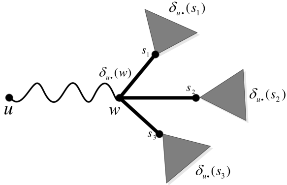
Figure 1. Illustration of Eq. (6). $w$ lies on shortest paths from source $u$ to $s_{1}$, $s_{2}$ and $s_{3}$, which are the successors of $w$ in the tree rooted at $u$. The figure is adapted from Figure 1 in (Brandes, 2001).

The algorithm performs a two-phase process. The first phase executes a shortest-path algorithm from $u$ to compute $\sigma_{uv}$ and $P_{u}(v)$ for all nodes $v$ with $v\neq u$. The second phase performs reversely from the leaves to the root and uses Eq. (6) to compute $\delta_{u\centerdot}(w)$. The whole process runs in $O(|V||E|)$ for unweighted networks and $O(|V||E|+|V|^{2}log|V|)$ for weighted networks, respectively, where $|V|$ and $|E|$ denote the number of nodes and edges in the network.

3.2. Notations

Let $G=(V,E)$ be a network with node features (attributes, structural features or arbitrary constant vectors) $X_{v}\in\mathbb{R}^{c}$ for $v\in V$, where $c$ denotes the dimension of input feature vectors, and $|V|$, $|E|$ be the number of nodes and edges respectively. $h_{v}^{(l)}\in\mathbb{R}^{p}\ (l=1,2,...,L)$ denotes the embedding of node $v$ at the $l-$th layer of the model, where $p$ is the dimension of hidden embeddings, which we assume to be the same across different layers for the sake of simplicity. We use $[d_{v},1,1]$ as node $v$’s initial feature $X_{v}$, and let $h_{v}^{(0)}=X_{v}$. The neighborhood of node $v$, $N(v)$, is defined as all the nodes that are adjacent to $v$, and $h_{N(v)}^{(l)}$ denotes the aggregated neighborhood representation output by the $l-$th layer of the model.

3.3.

We now introduce our model  in detail, which follows an encoder-decoder framework. Figure 2 illustrates the main architecture of . It consists of two components: 1) the encoder that generates node embeddings, and 2) the decoder that maps the embeddings to scalars for ranking nodes specified by BC values.

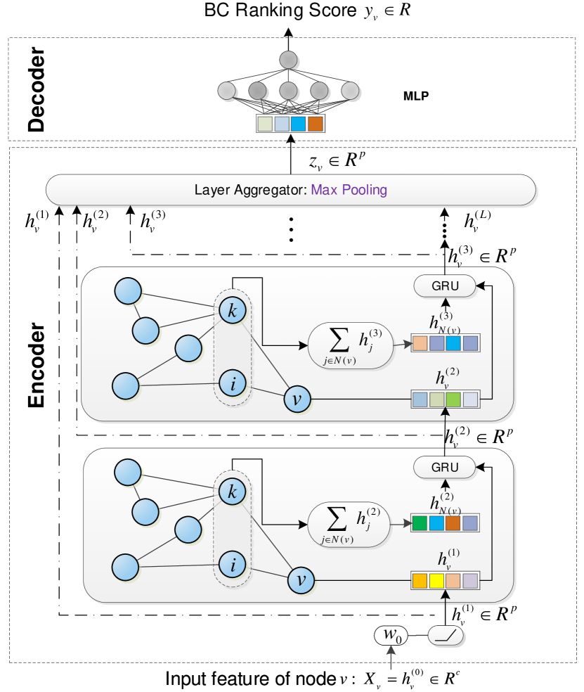
Figure 2. The encoder-decoder framework of

.

3.3.1. The Encoder.

As is indicated in Eq. (6) and Figure 1, computing a node’s exact BC value needs to iteratively aggregate its neighbors information, which is similar as the neighbor aggregation schema in graph neural networks. Therefore, we explore to choose GNNs as the encoder, and its inductive settings enable us to train on small-scale graphs and test directly on very large networks, which is the main reason for the efficiency of . For the specific design, we consider the following four components:

Neighborhood Definition. According to Eq. (6), the exact computation of the BC value of a node relies on its immediate neighbors. Therefore, we include all immediate neighbors of a node for full exploitation. Note that our model will be trained only on small networks, and utilizing all adjacent neighbors would not incur expensive computational burdens.

Neighborhood Aggregation. In Eq. (6), each neighbor is weighted by the term $\frac{\sigma_{uw}}{\sigma_{us}}$, where $\sigma_{ij}$ denotes the number of shortest paths from $i$ to $j$. As the number of shortest paths between two nodes is expensive to compute in large networks, we propose to use a weighted sum aggregator to aggregate neighbors, which is defined as follows :

(7) $$h_{N(v)}^{(l)}=\sum_{j\in N(v)}\frac{1}{\sqrt{d_{v}+1}\cdot\sqrt{d_{j}+1}}h_{j}^{(l-1)}$$

where $d_{v}$ and $d_{j}$ denote the degrees of node $v$ and node $j$, $h_{j}^{(l-1)}$ denotes node $j$’s embedding output by the $(l-1)$-th layer of the model. For the aggregator, the weight here is determined by the node’s degree, which is both efficient to compute and effective to describe its topological role in the network. Note that the attention mechanism (Velickovic et al., 2018) can also be used to automatically learn neighbors weights, which we leave as future work.

COMBINE Function. The $COMBINE$ function deals with the combination of the neighborhood embedding generated by the current layer, and the embedding of the node itself generated by the previous layer. Most existing models explore the forms of sum (Kipf and Welling, 2017) and concatenation (Hamilton et al., 2017a). Here we propose to use the GRU. Let the neighborhood embedding $h_{N(v)}^{(l)}$ generated by the $l$-th layer be the input state, and node $v$’s embedding $h_{v}^{(l-1)}$ generated by the $(l-1)$-th layer be the hidden state, then the embedding of node $v$ at the $l$-th layer can be written as $h_{v}^{(l)}=GRUCell(h_{v}^{(l-1)},h_{N(v)}^{(l)})$. The GRU utilizes the gating mechanism. The update gate $u_{l}$ helps the model determine how much past information needs to be passed along to the future, and the reset gate $r_{l}$ determines how much past information to be forgotten. Specifically, the GRU transition $GRUCell$ is given as the following:

(8) $$u_{l}=sigmoid(W_{1}h_{N(v)}^{(l)}+U_{1}h_{v}^{(l-1)})$$

(9) $$r_{l}=sigmoid(W_{2}h_{N(v)}^{(l)}+U_{2}h_{v}^{(l-1)})$$

(10) $$f_{l}=tanh(W_{3}h_{N(v)}^{(l)}+U_{3}(r_{l}\odot h_{v}^{(l-1)}))$$

(11) $$h_{v}^{(l)}=u_{l}\odot f_{l}+(1-u_{l})\odot h_{v}^{(l-1)}$$

where $\odot$ represents the element-wise product. With GRU, our model can learn to decide how much proportion of the features of distant neighbors should be incorporated into the local feature of each node. In comparison with other $COMBINE$ functions, GRU offers a more flexible way for feature selection, and gains a more accurate BC ranking in our experiments.

Layer Aggregation. As Li et al. (Li et al., 2018) point out that each propagation layer is simply a special form of smoothing which mixes the features of a node and its nearby neighbors. However, repeating the same number of iterations (layers) for all nodes would lead to over-smoothing or under-smoothing for different nodes with varying local structures. Some nodes with high BC values are located in the core part or within a few hops away from the core, and their neighbors thus can expand to nearly the entire network within few propagation steps. However, for those with low BC values, like nodes with degree one, their neighborhoods often cover much fewer nodes within the same steps. This implies that the same number of iterations for all nodes may not be reasonable, and wide-range or small-range propagation combinations based on local structures may be more desirable. Hence, Xu et al. (Xu et al., 2018) explore three layer-aggregation approaches: concatenation, max-pooling and LSTM-attention respectively. In this paper, we investigate the max-pooling aggregator, which is defined as an element-wise operation $max(h_{v}^{(1)},...,h_{v}^{(L)})$ to select the most informative (using $max$ operator) layer for each feature coordinate. This mechanism is adaptive and easy to be implemented, and it introduces no additional parameters to the learning process. In our experiments, we find it more effective than the other two layer aggregators for BC ranking. Practically, we set the maximum number of layers to be 5 when training, and more layers lead to no improvement.

Combining the above four components, we have the following encoder function:

(12) $$z_{v}=ENC(A,X;\Theta_{ENC})$$

where $A$ denotes the adjacency matrix, $X$ denotes node features, and $\Theta_{ENC}=\{W_{0}\in\mathbb{R}^{c\times p},W_{1},U_{1},W_{2},U_{2},W_{3},U_{3}\in\mathbb{R}^{p\times p}\}$. The detailed encoding process is shown in Algorithm 1.

Algorithm 1 encoder function

0:  Network $G=(V,E)$; input features $\{X_{v}\in\mathbb{R}^{c},\forall v\in V\}$; depth $L$; weight matrices $W_{0},W_{1},U_{1},W_{2},U_{2},W_{3},U_{3}$.

0:  Vector representations $z_{v}$, $\forall v\in V$.

1:  Initialize $h^{(0)}_{v}=X_{v}$;

2:  $h^{(1)}_{v}=ReLU(W_{0}h^{(0)}_{v})$, $h_{v}^{(1)}=h_{v}^{(1)}/\|h_{v}^{(1)}\|_{2},\forall v\in V$;

3:  for $l=2$ to $L$ do

4:     for $v\in V$ do

5:        $h_{N(v)}^{(l)}=\sum_{j\in N(v)}\frac{1}{\sqrt{d_{v}+1}\cdot\sqrt{d_{j}+1}}h_{j}^{(l-1)}$;

6:        $h_{v}^{(l)}=GRUCell(h_{v}^{(l-1)},h_{N(v)}^{(l)})$;

7:     end for

8:     $h_{v}^{(l)}=h_{v}^{(l)}/\|h_{v}^{(l)}\|_{2},\forall v\in V$;

9:  end for

10:  $z_{v}=max(h_{v}^{(1)},h_{v}^{(2)},...,h_{v}^{(L)}),\forall v\in V$;

3.3.2. The Decoder.

The decoder is implemented with a two-layered MLP which maps the embedding $z_{v}$ to the approximate BC ranking score $y_{v}$:

(13) $$y_{v}=DEC(z_{v};\Theta_{DEC})=W_{5}ReLU(W_{4}z_{v})$$

where $\Theta_{DEC}=\{W_{4}\in\mathbb{R}^{p\times q},W_{5}\in\mathbb{R}^{q}\}$, $p$ denotes the dimension of $z_{v}$, and $q$ is the number of hidden neurons.

3.4. Training Algorithm

There are two sets of parameters to be learned, including $\Theta_{ENC}$ and $\Theta_{DEC}$. We use the following pairwise ranking loss to update these parameters.

Given a node pair $(i,j)$, suppose the ground truth BC values are $b_{i}$ and $b_{j}$, respectively, our model predicts two corresponding BC ranking scores $y_{i}$ and $y_{j}$. Given $b_{ij}\equiv b_{i}-b_{j}$, since we seek to preserve the relative rank order specified by the ground truth, our model learn to infer $y_{ij}\equiv y_{i}-y_{j}$ based on the following binary cross-entropy cost function,

(14) $$C_{i,j}=-g(b_{ij})*log\sigma(y_{ij})-(1-g(b_{ij}))*log(1-\sigma(y_{ij}))$$

where $g(x)=1/(1+e^{-x})$. As such, the training loss is defined as:

(15) $$Loss=\sum_{i,j\in V}C_{i,j}$$

In our experiments, we randomly sample $5|V|$ source nodes and $5|V|$ target nodes with replacement, forming $5|V|$ random node pairs to compute the loss. Algorithm 2 describes the training algorithm for .

Algorithm 2 Training algorithm for

0:  Encoder parameters $\Theta_{ENC}=(W_{0},W_{1},U_{1},W_{2},U_{2},W_{3},U_{3})$, Decoder parameters $\Theta_{DEC}=(W_{4},W_{5})$

0:  Trained Model M

1:  for each episode do

2:     Draw network $G$ from distribution D (like the power-law model)

3:     Calculate each node’s exact BC value $b_{v},\forall v\in V$

4:     Get each node’s embedding $z_{v},\forall v\in V$ with Algorithm 1

5:     Compute BC ranking score $y_{v}$ for each node $v$ with Eq. (13)

6:     Sample source nodes and target nodes, and form a batch of node pairs

7:     Update $\Theta=(\Theta_{ENC},\Theta_{DEC})$ with Adam by minimizing Eq. (15)

8:  end for

3.5. Complexity Analysis

Training complexity. During training, the time complexity is proportional to the training iterations, which are hard to be theoretically analyzed. Empirically, our model can converge (measured by validation performance) very quickly, as is shown in Figure 3(A), and the convergence time seems to increase linearly with the training scale (Figure 3(B)). It is generally affordable to train the . For example, to train a model with a training scale of 4000-5000, which we utilize in the following experiments, its convergence time is about 4.5 hours (Figure 3(B), including the time to compute ground truth BC values for training graphs already). Notably, the training phase is performed only once here, and we can utilize the trained model for any input network in the application phase.

Inference complexity. In the application phase, we apply the trained   for a given network. The time complexity of the inference process is determined by two parts. The first is from the encoding phase. As shown in Algorithm 1, the encoding complexity takes $O(L|V|N(\cdot))$, where $L$ is the number of propagation steps, and usually is a small constant (e.g., 5), $V$ is the number of nodes, $N(\cdot)$ is the average number of node neighbors. In practice, we use the adjacency matrix multiplication for Line 4-8 in Algorithm 1, and due to the fact that most real-world networks are sparsely connected, the adjacency matrix in our setting is processed as a sparse matrix. As such, the encoding complexity in our implementations turns to be $O(|E|)$, where $E$ is the number of edges. The second is from the decoding phase. Once the nodes are encoded, we can compute their respective BC ranking score, and return the top-k highest BC nodes. the time complexity of this process mainly comes from the sorting operation, which takes $O(|V|)$. Therefore, the total time complexity for the inference phase should be $O(|E|+|V|+|V|log|V|)$.

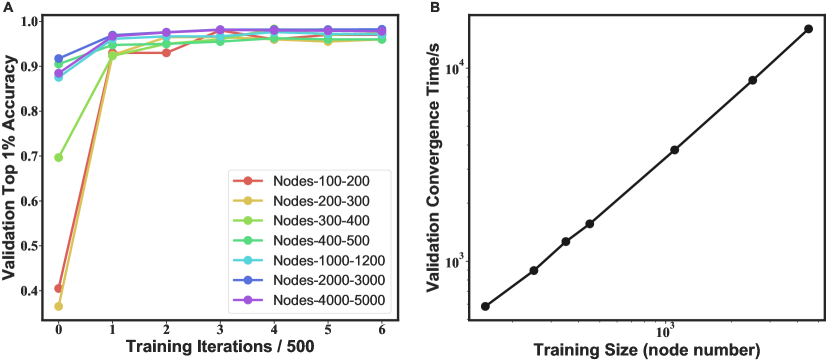
Figure 3. Training analysis of . (A).   convergence measured by validation top-1% accuracy. Different lines denote different models trained with the corresponding scale. (B).   convergence time for different training scales. We report all the time when training iterations reach 2500. The training size is the same as shown in (A).

4. Experiments

In this section, we demonstrate the effectiveness and efficiency of  on both synthetic and real-world networks. We start by illustrating the discriminative embeddings generated by different models. Then we explain experimental settings in detail, including baselines and datasets. After that, we discuss the results.

4.1. Case Study: Visualization of Embeddings

We employ the 2D PCA projection to visualize the learned embeddings to intuitively show that our model preserves the relative BC order between nodes in the embedding space. For comparison, we also show the results of the other two traditional node embedding models, i.e., Node2Vec (Grover and Leskovec, 2016) and GraphWave (Donnat et al., 2018). Although these two models are not designed for BC approximation, they can be used to identify the equivalent structural roles in the network, and we believe nodes with similar BC values share similar “bridge” roles that control the information flow on networks. As such, we compare against these two models to see whether they can maintain BC similarity as well. The example network is generated from the powerlaw-cluster model (Holme and Kim, 2002) (for which we use Networkx 1.11 and set the number of nodes $n=50$ and average degree $m=4$). For Node2Vec, let $p=1$, $q=2$ to enable it to capture the structural equivalence among nodes  (Grover and Leskovec, 2016). For GraphWave, we use the default settings in (Donnat et al., 2018). As for , we use the same model tested in the following experiments. All embedding dimensions are set to be 128. As is shown in Figure 4, only in (D), the linear separable portions correspond to clusters of nodes with similar BC, while the other two both fail to make it. This indicates that  could generate more discriminative embeddings for BC prediction, which may provide some intuitions behind its prediction accuracy shown in the following experiments.

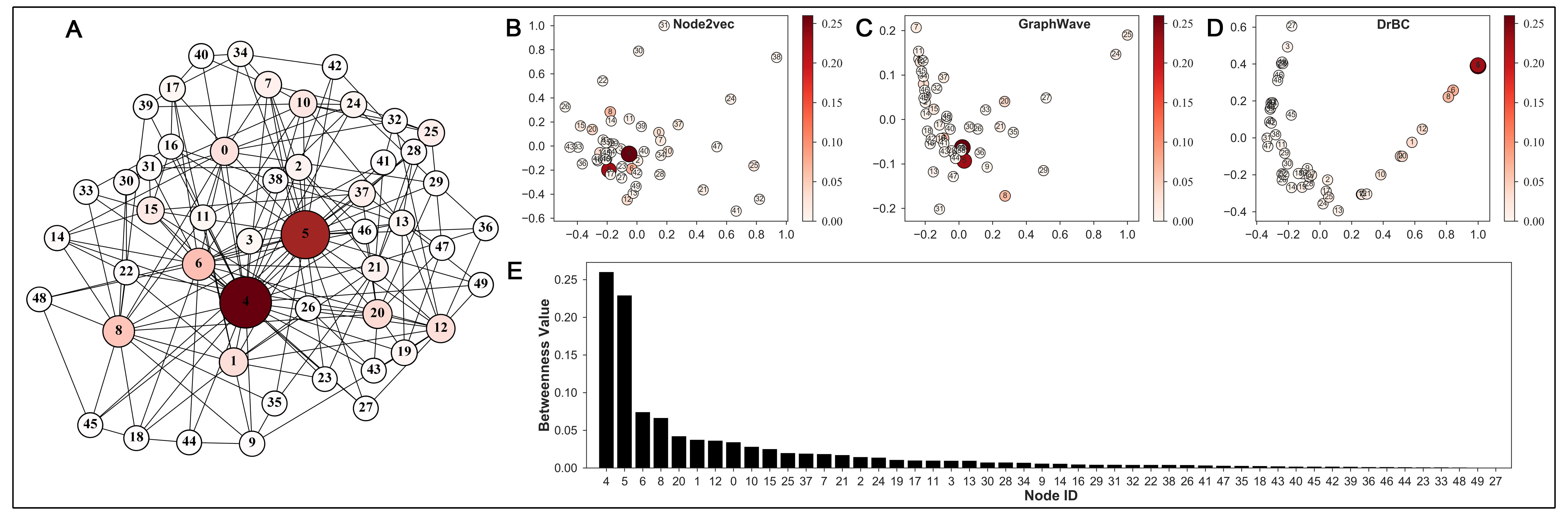
Figure 4. The case network with 50 nodes and 200 edges, nodes with larger BC values having darker colors and larger shapes (A). 2D PCA projection of embeddings learned by Node2Vec (B), GraphWave (C) and   (D). BC value distribution of the case network (descending order) (E).

4.2. Experimental Setup

4.2.1. Baseline Methods.

We compare  with three approximation algorithms which focus on estimating exact BC values, i.e., ABRA, RK, k-BC, one approximation which seeks to identify top-$N\%$ highest BC nodes, i.e., KADABRA, and one traditional node embedding model, Node2Vec. Details of these baselines are described as follows:

• ABRA (Riondato and Upfal, 2018). ABRA keeps sampling node pairs until the desired level of accuracy is reached. We use the parallel implementation by Riondato and Upfal (Riondato and Upfal, 2018) and Staudt et al. (Staudt et al., 2016). We set the error tolerance $\lambda$ to 0.01 and the probability $\delta$ to 0.1, following the setting in (Riondato and Upfal, 2018).

• RK (Riondato and Kornaropoulos, 2016). RK determines the required sample size based on the diameter of the network. We adopt the implementation in the NetworKit library (Staudt et al., 2016). We set the error tolerance $\lambda$ to 0.01 and the probability $\delta$ to 0.1.

• k-BC (Pfeffer and Carley, 2012). k-BC bounds the traversals of Brandes algorithm (Brandes, 2001) by $k$ steps. For the value of $k$, we set it to be $20\%$ of the diameter of the network.

• KADABRA (Borassi and Natale, 2016). KADABRA follows the idea of adaptive sampling and proposes balanced bidirectional BFS to sample the shortest paths. We use its variant well designed for computing top-$N\%$ highest BC nodes. We set the error tolerance and probability the same as ABRA and RK.

• Node2Vec (Grover and Leskovec, 2016). Node2Vec designs a biased random walk procedure to explore a node’s diverse neighbors, and learns each node’s embedding vector that maximizes the likelihood of preserving its neighbors. Node2Vec can efficiently learn task-independent representations which are highly related to the network structure. In our experiments, we set $p$=1 and $q$=2 to enable Node2Vec to capture the structural equivalence of nodes, since BC can be viewed as a measure of “bridge“ role on networks. We train a MLP to map Node2Vec embeddings to BC ranking scores, following the same training procedure as Algorithm 2. At the test stage, this baseline generates Node2Vec embeddings and then applies the trained MLP to obtain the ranking score for each node.

4.2.2. Datasets.

We evaluate the performance of  on both synthetic networks and large real-world ones. For synthetic networks, we generate them with the powerlaw-cluster model (Holme and Kim, 2002), which generates graphs that could capture both powerlaw degree distribution and small-world phenomenon, and most real-world networks conform to these two properties. The basic parameters of this model are average degree $m=4$ and the probability of adding a triangle after adding a random edge $p=0.05$. We keep them the same when generating synthetic graphs with six different scales: 5000, 10000, 20000, 50000 and 100000. For real-world test data, we use five large real-world networks provided by AlGhamdi et al. (AlGhamdi et al., 2017). Descriptions of these networks are as follows and Table 1 summarizes their statistics.

com-Youtube is a video-sharing web site that includes a social network. Nodes are users and edges are friendships.

Amazon is a product network created by crawling the Amazon online store. Nodes represent products and edges link commonly co-purchased products.

Dblp is an authorship network extracted from the DBLP computer science bibliography. Nodes are authors and publications. Each edge connects an author to one of his publications.

cit-Patents is a citation network of U.S. patents. Nodes are patents and edges represent citations. In our experiments, we regard it as an undirected network.

com-lj is a social network where nodes are LiveJournal users and edges are their friendships.

Table 1. Summary of real-world datasets.

Network	—V—	—E—	Average Degree	Diameter
com-Youtube	1,134,890	2,987,624	5.27	20
Amazon	2,146,057	5,743,146	5.35	28
Dblp	4,000,148	8,649,011	4.32	50
cit-Patents	3,764,117	16,511,741	8.77	26
com-lj	3,997,962	34,681,189	17.35	17

4.2.3. Ground Truth Computation.

We exploit the graph-tool library (Peixoto, 2014) to compute the exact BC values for synthetic networks. For real-world networks, we use the exact BC values reported by AlGhamdi et al. (AlGhamdi et al., 2017), which are computed via a parallel implementation of Brandes algorithm using a 96,000-core supercomputer.

4.2.4. Evaluation Metrics.

For all baseline methods and , we report their effectiveness in terms of top-$N\%$ accuracy and kendall tau distance, and their efficiency in terms of wall-clock running time.

Top-$N\%$ accuracy is defined as the percentage of overlap between the top-$N\%$ nodes as returned by an approximation method and the top-$N\%$ nodes as identified by Brandes algorithm (ground truth):

$$\text{Top-}N\%=\frac{|\{\text{returned top-}N\%\text{nodes}\}\cap\{\text{true top-}N\%\text{nodes}\}|}{\lceil|V|\times N\%\rceil}$$

where $|V|$ is the number of nodes, and $\lceil x\rceil$ is the ceiling function. In our paper, we mainly compare top-$1\%$, top-$5\%$ and top-$10\%$.

Kendall tau distance is a metric that calculates the number of disagreements between the rankings of the compared methods.

$$K(\tau_{1},\tau_{2})=\frac{2(\alpha-\beta)}{n*(n-1)}$$

where $\alpha$ is the number of concordant pairs, and $\beta$ is the number of discordant pairs. The value of kendall tall distance is in the range [-1, 1], where 1 means that two rankings are in total agreement, while -1 means that the two rankings are in complete disagreement. Wall-clock running time is defined as the actual time taken from the start of a computer program to the end, usually in seconds.

4.2.5. Other Settings.

All the experiments are conducted on a 80-core server with 512GB memory, and 8 16GB Tesla V100 GPUs. Notably, we train  with the GPUs while test it with only CPUs for a more fair time comparison with the baselines, since most baselines do not utilize the GPU environment. We generate 10,000 synthetic networks at random for training, and 100 for validation. We adopt early stopping to choose the best model based on validation performance. The model is implemented in Tensorflow with the Adam optimizer, and values of hyper-parameters (Table 2) are determined according to the performance on the validation set. The trained model and the implementation codes are released at https://github.com/FFrankyy/DrBC.

Table 2. Hyper-parameter configuration for .

Hyper-parameter	Value	Description
learning rate	0.0001	the learning rate used by Adam optimizer
embedding dimension	128	dimension of node embedding vector
mini-batch size	16	size of mini-batch training samples
average node sampling times	5	average sampling times per node for training
maximum episodes	10000	maximum episodes for the training process
layer iterations	5	number of neighborhood-aggregation iterations

Table 3. Top-$N\%$ accuracy ($\times 0.01$) on synthetic graphs of different scales. The bold results indicate the best among all methods. For each scale, we report the mean and standard deviation over 30 tests.

Scale	Top-$1\%$						Top-$5\%$						Top-$10\%$
	ABRA	RK	k-BC	KADABRA	Node2Vec		ABRA	RK	k-BC	KADABRA	Node2Vec		ABRA	RK	k-BC	KADABRA	Node2Vec
5000	97.8$\pm$1.5	96.8$\pm$1.7	94.1$\pm$0.8	76.2$\pm$12.5	19.1$\pm$4.8	96.5$\pm$1.8	96.9$\pm$0.7	95.6$\pm$0.9	89.3$\pm$3.9	68.7$\pm$13.4	23.3$\pm$3.6	95.9$\pm$0.9	96.1$\pm$0.7	94.3$\pm$0.9	86.7$\pm$4.5	67.2$\pm$12.5	25.4$\pm$3.4	94.8$\pm$0.7
10000	97.2$\pm$1.2	96.4$\pm$1.3	93.3$\pm$3.1	74.6$\pm$16.5	21.2$\pm$4.3	96.7$\pm$1.2	95.6$\pm$0.8	94.1$\pm$0.8	88.4$\pm$5.1	70.7$\pm$13.8	20.5$\pm$2.7	95.0$\pm$0.8	94.1$\pm$0.6	92.2$\pm$0.9	86.0$\pm$5.9	67.8$\pm$13.0	25.4$\pm$3.4	94.0$\pm$0.9
20000	96.5$\pm$1.0	95.5$\pm$1.1	91.6$\pm$4.0	74.6$\pm$16.7	16.1$\pm$3.9	95.6$\pm$0.9	93.9$\pm$0.8	92.2$\pm$0.9	86.9$\pm$6.2	69.1$\pm$13.5	16.9$\pm$2.0	93.0$\pm$1.1	92.1$\pm$0.8	90.6$\pm$0.9	84.5$\pm$6.8	66.1$\pm$12.4	19.9$\pm$1.9	91.9$\pm$0.9
50000	94.6$\pm$0.7	93.3$\pm$0.9	90.1$\pm$4.7	73.8$\pm$14.9	9.6$\pm$1.3	92.5$\pm$1.2	90.1$\pm$0.8	88.0$\pm$0.8	84.4$\pm$7.2	65.8$\pm$11.7	13.8$\pm$1.0	89.2$\pm$1.1	87.4$\pm$0.9	88.2$\pm$0.5	82.1$\pm$8.0	61.3$\pm$10.4	18.0$\pm$1.2	87.9$\pm$1.0
100000	92.2$\pm$0.8	91.5$\pm$0.8	88.6$\pm$4.7	67.0$\pm$12.4	9.6$\pm$1.3	90.3$\pm$0.9	85.6$\pm$1.1	87.6$\pm$0.5	82.4$\pm$7.5	57.0$\pm$9.4	12.9$\pm$1.2	86.2$\pm$0.9	81.8$\pm$1.5	87.4$\pm$0.4	80.1$\pm$8.2	52.4$\pm$8.2	17.3$\pm$1.3	85.0$\pm$0.9

Table 4. Kendall tau distance ($\times 0.01$) on synthetic graphs. (Since KADABRA only outputs the top-$N\%$ nodes, we cannot obtain the kendall tau distance for the overall ranking list.)

	ABRA	RK	k-BC	KADABRA	Node2Vec
5000	86.6$\pm$1.0	78.6$\pm$0.6	66.2$\pm$11.4	NA	11.3$\pm$3.0	88.4$\pm$0.3
10000	81.6$\pm$1.2	72.3$\pm$0.6	67.2$\pm$13.5	NA	8.5$\pm$2.3	86.8$\pm$0.4
20000	76.9$\pm$1.5	65.5$\pm$1.2	67.1$\pm$14.3	NA	7.5$\pm$2.2	84.0$\pm$0.5
50000	68.2$\pm$1.3	53.3$\pm$1.4	66.2$\pm$14.1	NA	7.1$\pm$1.8	80.1$\pm$0.5
100000	60.3$\pm$1.9	44.2$\pm$0.2	64.9$\pm$13.5	NA	7.1$\pm$1.9	77.8$\pm$0.4

4.3. Results on Synthetic Networks

We report the top-$N\%$ (1,5,10) accuracy, kendall tau distance and running time of baselines and  on synthetic networks with different scales, as shown in Table 3, 4 and 5. For each scale, we generate 30 networks at random for testing and report the mean and standard deviation. For ABRA, RK and KADABRA, we independantly run 5 times each on all the test graphs. The   model is trained on powerlaw-cluster graphs with node sizes in 4000-5000.

Table 5. Running time comparison on synthetic networks.

	ABRA	RK	k-BC	KADABRA	Node2Vec
5000	18.5$\pm$3.6	17.1$\pm$3.0	12.2$\pm$6.3	0.6$\pm$0.1	32.4$\pm$3.8	0.3$\pm$0.0
10000	29.2$\pm$4.8	21.0$\pm$3.6	47.2$\pm$27.3	1.0$\pm$0.2	73.1$\pm$7.0	0.6$\pm$0.0
20000	52.7$\pm$8.1	43.0$\pm$3.2	176.4$\pm$105.1	1.6$\pm$0.3	129.3$\pm$17.6	1.4$\pm$0.0
50000	168.3$\pm$23.8	131.4$\pm$2.0	935.1$\pm$505.9	3.9$\pm$1.0	263.2$\pm$46.6	3.9$\pm$0.2
100000	380.3$\pm$63.7	363.4$\pm$36.3	3069.2$\pm$1378.5	7.2$\pm$1.8	416.2$\pm$37.0	8.2$\pm$0.3

Table 6. ’s generalization results on different scales (Top-$1\%$ accuracy, $\times 0.01$).

	5000	10000	20000	50000	100000
100_200	90.5$\pm$2.9	88.3$\pm$2.1	85.5$\pm$1.9	83.9$\pm$1.1	82.2$\pm$0.9
200_300	92.5$\pm$2.7	90.0$\pm$2.2	87.0$\pm$2.1	84.8$\pm$1.1	82.9$\pm$0.9
1000_1200	94.3$\pm$2.2	90.6$\pm$1.7	87.8$\pm$1.9	85.1$\pm$1.1	83.1$\pm$0.9
2000_3000	95.7$\pm$1.8	93.5$\pm$1.7	90.7$\pm$1.6	87.8$\pm$1.1	85.9$\pm$0.7
4000_5000	96.5$\pm$1.8	96.7$\pm$1.2	95.6$\pm$0.9	92.5$\pm$1.2	90.3$\pm$0.9

Table 7. ’s generalization results on different scales (kendall tau distance, $\times 0.01$).

	5000	10000	20000	50000	100000
100_200	43.6$\pm$1.0	40.1$\pm$0.6	37.5$\pm$0.5	35.2$\pm$0.3	33.9$\pm$0.2
200_300	42.7$\pm$0.8	39.5$\pm$0.5	37.1$\pm$0.5	35.0$\pm$0.3	33.9$\pm$0.2
1000_1200	56.4$\pm$0.6	42.7$\pm$0.4	36.0$\pm$0.4	31.7$\pm$0.3	29.8$\pm$0.2
2000_3000	86.1$\pm$0.3	78.1$\pm$0.5	69.9$\pm$0.6	62.3$\pm$0.5	59.1$\pm$0.3
4000_5000	88.4$\pm$0.3	86.8$\pm$0.4	84.0$\pm$0.5	80.1$\pm$0.5	77.8$\pm$0.4

Table 8. Top-$N\%$ accuracy ($\times 0.01$) and running time on large real-world networks. *result is adopted from (AlGhamdi et al., 2017), since RK can not finish within the acceptable time. The bold results indicate the best performance of the network under the current metric.

Network	Top-$1\%$					Top-$5\%$					Top-$10\%$					Time/s
	ABRA	RK	KADABRA	Node2Vec		ABRA	RK	KADABRA	Node2Vec		ABRA	RK	KADABRA	Node2Vec		ABRA	RK	KADABRA	Node2Vec
com-youtube	95.7	76.0	57.5	12.3	73.6	91.2	75.8	47.3	18.9	66.7	89.5	100.0	44.6	23.6	69.5	72898.7	125651.2	116.1	4729.8	402.9
amazon	69.2	86.0	47.6	16.7	86.2	58.0	59.4	56.0	23.2	79.7	60.3	100.0	56.7	26.6	76.9	5402.3	149680.6	244.7	10679.0	449.8
Dblp	49.7	NA	35.2	11.5	78.9	45.5	NA	42.6	20.2	72.0	100.0	NA	50.4	27.7	72.5	11591.5	NA	398.1	17446.9	566.7
cit-Patents	37.0	74.4	23.4	0.04	48.3	42.4	68.2	25.1	0.29	57.5	50.9	53.5	21.6	0.99	64.1	10704.6	252028.5	568.0	11729.1	744.1
com-lj	60.0	54.2*	31.9	3.9	67.2	56.9	NA	39.5	10.35	72.6	63.6	NA	47.6	15.4	74.8	34309.6	NA	612.9	18253.6	2274.2

We can see from Table 3, 4 and 5 that,   achieves competitive top-$N\%$ accuracy compared with the best approximation results, and outperforms all baselines in terms of the kendall tau distance. Running time comparison shows the obvious efficiency advantage. Take graphs with size 100000 as an example, although  sacrifices about 2% loss in top-$1\%$ accuracy compared with the best result (ABRA), it is over 46 times faster. It is noteworthy that we do not consider the training time here. Since none of the approximation algorithms requires training, it may cause some unfair comparison. However, considering that  only needs to be trained once offline and can then generalize to any unseen network, it is reasonable not to consider the training time in comparison. As analyzed in section 3.5,  can converge rapidly, resulting in acceptable training time, e.g., it takes about 4.5 hours to train and select the model used in this paper.

Overall, ABRA achieves the highest top-$N\%$ accuracy, and RK is very close to ABRA in accuracy and time, while k-BC is far worse in terms of both effectiveness and efficiency. KADABRA is designed to identify the top-$N\%$ highest BC nodes, so it only outputs the top-$N\%$ nodes, making it impossible to calculate the kendall tau distance for the whole ranking list. We can see from Table 5 that KADABRA is very efficient, which is close to , however, its high efficiency sacrifices too much accuracy, over 20% lower than  on average. We also observe that Node2Vec performs very poor in this task, which may due to that Node2Vec learns task-independent representations which only capture nodes’ local structural information, while BC is a measure highly related to the global. In our model, we train it in an end-to-end manner, enabling the ground truth BC relative order to shape the learned representations. Experiments demonstrate that learning in this way can capture better informative features related to BC. For the kendall tau distance metric which measures the quality of the whole ranking list,  performs significantly better than the other baselines. This is because  learns to maintain the relative order between nodes specified by true BC values, while other baselines either focus on approximating exact BC values or seek to identify the top-$N\%$ highest BC nodes.

The inductive setting of  enables us to train and test our model on networks of different scales, since the model’s parameters are independent of the network scale. Table 3 and 4 have already verified that our model can generalize to larger graphs than what they are trained on. Here we show the model’s full generalizability by training on different scales and compare the generalizability for each scale. As is shown in Table 6 and 7 which illustrate results of top-$1\%$ accuracy and kendall tau distance, the model can generalize well on larger graphs for each scale, and it seems that model trained on larger scales can achieve better generalization results. The intuition behind is that larger scale graphs represent more difficult samples, making the learned model more generalizable. This observation may inspire us to train on larger scales to improve the performance on very large real-world networks. In this paper, we just use the model trained with node sizes in 4000-5000 and test on the following five large real-world networks.

4.4. Results on Real-world Networks

In section 4.3, we test  on synthetic graphs generated from the same model as it is trained on, and we have observed it can generalize well on those larger than the training scale. In this section, we test  on different large-scale real-world networks to see whether it is still generalizable in practice.

We compare top-$N\%$ accuracy, kendall tau distance and running time in Table 8 and 9. Since k-BC cannot obtain results within the acceptable time on these networks, we do not compare against it here. RK cannot finish within 3 days for Dblp and com-lj, so we just use its top-$1\%$ accuracy on com-lj reported in (AlGhamdi et al., 2017). Due to the time limits, for ABRA and RK, we only run once on each network. For KADABRA and , we independently run five times for each network and report the averaged accuracy and time.

Table 9. Kendall tau distance ($\times 0.01$) on real-world networks. (Since KADABRA only outputs top-$N\%$ nodes, we cannot obtain the kendall tau distance for the overall ranking list. RK did not finish on Dblp and com-lj within the acceptable time.)

	ABRA	RK	KADABRA	Node2Vec
com-youtube	56.2	13.9	NA	46.2	57.3
amazon	16.3	9.7	NA	44.7	69.3
Dblp	14.3	NA	NA	49.5	71.9
cit-Patents	17.3	15.3	NA	4.0	72.6
com-lj	22.8	NA	NA	35.1	71.3

We can see in Table 8 that different methods perform with a large variance on different networks. Take ABRA as an example, it can achieve 95.7% top 1% accuracy on com-youtube, while only 37.0% on cit-Patents. It seems that no method can achieve consistent overwhelming accuracy than others. However, if we consider the trade-off between accuracy and efficiency, our model performs the best, especially for the latter, which is several orders of magnitude faster than ABRA and RK. Besides efficiency,  actually performs on par with or better than these approximation algorithms in terms of accuracy. Specifically,   achieves the best top-$1\%$ and top-$5\%$ accuracy in three out of the five networks. KADABRA is the most efficient one, while accompanied by too much accuracy loss. Node2Vec performs the worst, with the worst accuracy and relatively longer running time. In terms of the kendall tau distance,  consistently performs the best among all methods (Table 9).

Table 10. Effect of different training graph types on synthetic graphs (%). For each type, node sizes of the training graphs and test graphs both lie between 100-200. We report the mean and standard deviations over 100 tests.

	ER	BA	PL-cluster
ER	87.0$\pm$33.6	82.0$\pm$38.4	84.0$\pm$36.7
BA	62.5$\pm$48.2	93.0$\pm$25.5	93.0$\pm$25.5
PL-cluster	73.5$\pm$43.9	96.0$\pm$19.6	96.0$\pm$19.6

Table 11. Effect of different training graph types on real networks (%).

	com-youtube	amazon	Dblp	cit-Patents	com-lj
ER	66.58	73.88	64.82	38.51	54.26
BA	72.92	70.89	73.87	35.56	55.08
PL-cluster	73.60	86.15	78.92	48.31	67.17

5. Discussion

In this section, we discuss the potential reasons behind ’s success. Since it’s hard to prove GNN’s theoretical approximation bound, we explain by giving the following observations:

(1) The exact BC computation method, i.e. Brandes algorithm, inherently follows a similar neighbor aggregation schema (Eq. (6)) as our encoder, despite that their neighbors are on the shortest paths. We believe this common trait enables our model to capture characteristics that are essential to BC computation;

(2) Our model limits graph exploration to a neighborhood of $L$-hops around each node, where $L$ denotes iterations of neighbor aggregation. The idea of using the $L$-hop sub-structure to approximate exact BC values is the basis of many existing BC approximation algorithms, such as EGO (Everett and Borgatti, 2005) and $\kappa$-path (Kourtellis et al., 2013).

(3) We train the model in an end-to-end manner with exact BC values as the ground truth. Like other successful deep learning applications on images or texts, if given enough training samples with ground truth, the model is expected to be able to learn well.

(4) The model is trained on synthetic graphs from the powerlaw-cluster (PL-cluster) model, which possesses the characteristics of power-law degree distribution and small-world phenomenon (large clustering coefficient), both of which appear in most real-world networks. In Table 10, we train  on Erdős-Rényi (ER) (Erdős and Rényi, 1959), Barabási-Albert (BA) (Barabási and Albert, 1999) and PL-cluster (Holme and Kim, 2002) graphs, and test each on different types. The results show that  always performs the best when the training type is the same as the testing type, and the PL-cluster training type enables better generalizations for  over the other two types. Table 11 further confirms this conclusion on real-world networks.

6. Conclusion and Future Work

In this paper, we for the first time investigate the power of graph neural networks in identifying high betweenness centrality nodes, which is a traditional but significant problem essential to many applications but often computationally prohibitive on large networks with millions of nodes. Our model is constituted with a neighborhood-aggregation encoder and a multi-layer perceptron decoder, and naturally applies to inductive settings where training and testing are independent. Extensive experiments on both synthetic graphs and large real-world networks show that our model can achieve very competitive accuracy while possessing a huge advantage in terms of running time. Notably, the presented results also highlight the importance of classical network models, such as the powerlaw-cluster model. Though extremely simple, it captures the key features, i.e., degree heterogeneity and small-world phenomenon, of many real-world networks. This tends out to be extremely important to train a deep learning model to solve very challenging problems on complex real networks.

There are several future directions for this work, such as exploring theorectical guarantees, applying it to some BC-related downstream applications (e.g. community detection and network attack) and extending the framework to approximate other network structural measures.

- (1)
- AlGhamdi et al. (2017) Ziyad AlGhamdi, Fuad Jamour, Spiros Skiadopoulos, and Panos Kalnis. 2017. A benchmark for betweenness centrality approximation algorithms on large graphs. In SSDBM. 6.
- Bai et al. (2018) Yunsheng Bai, Hao Ding, Song Bian, Yizhou Sun, and Wei Wang. 2018. Graph Edit Distance Computation via Graph Neural Networks. arXiv preprint arXiv:1808.05689 (2018).
- Barabási and Albert (1999) Albert-László Barabási and Réka Albert. 1999. Emergence of scaling in random networks. science 286, 5439 (1999), 509–512.
- Borassi and Natale (2016) Michele Borassi and Emanuele Natale. 2016. KADABRA is an ADaptive Algorithm for Betweenness via Random Approximation. In ESA.
- Brandes (2001) Ulrik Brandes. 2001. A faster algorithm for betweenness centrality. Journal of mathematical sociology 25, 2 (2001), 163–177.
- Braunstein et al. (2016) Alfredo Braunstein, Luca Dall’Asta, Guilhem Semerjian, and Lenka Zdeborová. 2016. Network dismantling. PNAS 113, 44 (2016).
- Chen et al. (2018) Haochen Chen, Xiaofei Sun, Yingtao Tian, et al. 2018. Enhanced Network Embeddings via Exploiting Edge Labels. In CIKM.
- Chen and Sun (2017) Ting Chen and Yizhou Sun. 2017. Task-guided and path-augmented heterogeneous network embedding for author identification. In WSDM.
- Chung and Lee (2014) Chin-Wan Chung and Min-joong Lee. 2014. Finding k-highest betweenness centrality vertices in graphs. In 23rd International World Wide Web Conference. International World Wide Web Conference Committee, 339–340.
- Donnat et al. (2018) Claire Donnat, Marinka Zitnik, David Hallac, and Jure Leskovec. 2018. Learning Structural Node Embeddings via Diffusion Wavelets. (2018).
- Erdős and Rényi (1959) P Erdős and A Rényi. 1959. On random graphs I. Publ. Math. Debrecen 6 (1959).
- Everett and Borgatti (2005) Martin Everett and Stephen P Borgatti. 2005. Ego network betweenness. Social networks 27, 1 (2005), 31–38.
- Fan et al. (2017) Changjun Fan, Zhong Liu, Xin Lu, Baoxin Xiu, and Qing Chen. 2017. An efficient link prediction index for complex military organization. Physica A: Statistical Mechanics and its Applications 469 (2017), 572–587.
- Fan et al. (2014) Changjun Fan, Kaiming Xiao, Baoxin Xiu, and Guodong Lv. 2014. A fuzzy clustering algorithm to detect criminals without prior information. In Proceedings of the 2014 IEEE/ACM International Conference on Advances in Social Networks Analysis and Mining. IEEE Press, 238–243.
- Grover and Leskovec (2016) Aditya Grover and Jure Leskovec. 2016. node2vec: Scalable feature learning for networks. In KDD.
- Hamilton et al. (2017a) Will Hamilton, Zhitao Ying, and Jure Leskovec. 2017a. Inductive representation learning on large graphs. In NIPS.
- Hamilton et al. (2017b) William L Hamilton, Rex Ying, and Jure Leskovec. 2017b. Representation learning on graphs: Methods and applications. arXiv (2017).
- Holme and Kim (2002) Petter Holme and Beom Jun Kim. 2002. Growing scale-free networks with tunable clustering. Physical review E 65, 2 (2002), 026107.
- Holme et al. (2002) Petter Holme, Beom Jun Kim, Chang No Yoon, and Seung Kee Han. 2002. Attack vulnerability of complex networks. Physical review E 65, 5 (2002), 056109.
- Kipf and Welling (2017) Thomas N Kipf and Max Welling. 2017. Semi-supervised classification with graph convolutional networks. In ICLR.
- Kourtellis et al. (2013) Nicolas Kourtellis, Tharaka Alahakoon, Ramanuja Simha, Adriana Iamnitchi, and Rahul Tripathi. 2013. Identifying high betweenness centrality nodes in large social networks. Social Network Analysis and Mining 3, 4 (2013).
- Kumbhare et al. (2014) Alok Gautam Kumbhare, Marc Frincu, Cauligi S Raghavendra, and Viktor K Prasanna. 2014. Efficient extraction of high centrality vertices in distributed graphs. In HPEC. IEEE, 1–7.
- Li et al. (2018) Qimai Li, Zhichao Han, and Xiao-Ming Wu. 2018. Deeper Insights into Graph Convolutional Networks for Semi-Supervised Learning. arXiv (2018).
- Li et al. (2016) Yujia Li, Daniel Tarlow, Marc Brockschmidt, and Richard Zemel. 2016. Gated graph sequence neural networks. In ICLR.
- Mahmoody et al. (2016) Ahmad Mahmoody, Charalampos E Tsourakakis, and Eli Upfal. 2016. Scalable betweenness centrality maximization via sampling. In KDD.
- Mahyar et al. (2018) Hamidreza Mahyar, Rouzbeh Hasheminezhad, Elahe Ghalebi, Ali Nazemian, Radu Grosu, Ali Movaghar, and Hamid R Rabiee. 2018. Compressive sensing of high betweenness centrality nodes in networks. Physica A: Statistical Mechanics and its Applications 497 (2018), 166–184.
- Newman (2006) Mark EJ Newman. 2006. Modularity and community structure in networks. PNAS 103, 23 (2006).
- Peixoto (2014) Tiago P Peixoto. 2014. The graph-tool python library. figshare (2014).
- Perozzi et al. (2014) Bryan Perozzi, Rami Al-Rfou, and Steven Skiena. 2014. Deepwalk: Online learning of social representations. In KDD.
- Pfeffer and Carley (2012) Jürgen Pfeffer and Kathleen M Carley. 2012. k-centralities: Local approximations of global measures based on shortest paths. In WWW.
- Riondato and Kornaropoulos (2016) Matteo Riondato and Evgenios M Kornaropoulos. 2016. Fast approximation of betweenness centrality through sampling. DMKD 30, 2 (2016).
- Riondato and Upfal (2018) Matteo Riondato and Eli Upfal. 2018. ABRA: Approximating betweenness centrality in static and dynamic graphs with rademacher averages. TKDD 12, 5 (2018).
- Staudt et al. (2016) Christian L Staudt, Aleksejs Sazonovs, and Henning Meyerhenke. 2016. NetworKit: A tool suite for large-scale complex network analysis. Network Science 4, 4 (2016), 508–530.
- Tang et al. (2015) Jian Tang, Meng Qu, Mingzhe Wang, Ming Zhang, Jun Yan, and Qiaozhu Mei. 2015. Line: Large-scale information network embedding. In WWW.
- Velickovic et al. (2018) Petar Velickovic, Guillem Cucurull, Arantxa Casanova, Adriana Romero, Pietro Lio, and Yoshua Bengio. 2018. Graph attention networks. In ICLR.
- Xu et al. (2018) Keyulu Xu, Chengtao Li, Yonglong Tian, Tomohiro Sonobe, Ken-ichi Kawarabayashi, and Stefanie Jegelka. 2018. Representation Learning on Graphs with Jumping Knowledge Networks. In ICML.
- Yoshida (2014) Yuichi Yoshida. 2014. Almost linear-time algorithms for adaptive betweenness centrality using hypergraph sketches. In KDD.