The statistical properties of turbulence in the presence of a smart small-scale control

Abstract

By means of high-resolution numerical simulations, we compare the statistical properties of homogeneous and isotropic turbulence to those of the Navier-Stokes equation where small-scale vortex filaments are strongly depleted, thanks to a non-linear extra viscosity acting preferentially on high vorticity regions. We show that the presence of such smart small-scale drag can strongly reduce intermittency and non-Gaussian fluctuations. Our results pave the way towards a deeper understanding on the fundamental role of degrees of freedom in turbulence as well as on the impact of (pseudo)coherent structures on the statistical small-scale properties. Our work can be seen as a first attempt to develop smart-Lagrangian forcing/drag mechanisms to control turbulence.

I Introduction

Fluid dynamics turbulence is characterized by intermittent and non-Gaussian fluctuations distributed over a wide range of space- and time-scales Frisch (1995); Benzi et al. (2010); yeung2015extreme ; Iyer et al. (2017); Sinhuber et al. (2017); Pope (2001). In the limit of infinite Reynolds numbers, $Re$, the number of dynamical degrees of freedom tends towards infinity, $\#_{dof}\sim Re^{9/4}$, where $Re=U_{0}L_{0}/\nu$ with $\nu$ the viscosity, $U_{0}$ and $L_{0}$ the typical velocity and large-scale in the flow, respectively. Are all these degrees of freedom equally relevant for the dynamics? Do extreme events depend only on some large-scale flow realizations? Can we selectively control some degrees-of-freedom by applying an active forcing and/or drag? These are key questions that we start to answer by using high resolution numerical studies of the three dimensional Navier-Stokes equations. The long term goal is twofold. First, we are interested to have a new numerical tool to ask novel questions concerning the statistical and topological properties of specific flow structures. Second, we aim to develop useful (optimal) control strategies to suggest forcing protocols that may be implemented in laboratory experiments, where the flow can be seeded with millions of passive or active particles, preferentially tracking special flow regions bec2007heavy ; toschi2009lagrangian ; calzavarinijfm2009 ; qureshi2008 ; mercado2010 ; gibert2012 ; gustavsson2016 ; mathai2016 . For example, we nowadays know how to actively control spinning properties of small magnetic particles Stanway04 ; Falcon17 , how to blow-up small bubbles by sound emissions abe02 ; hauptmann13 ; hauptmann14 and/or how to assemble micro-metric objects with a self-adaptive shape depending on the flow rheological properties huang2019 . Recent developments in 3d-printing and micro-engineering technologies promise that new tools will be available in the next few years for fluid control or fluid measurements in the laboratory. We believe that these new tools could be capable to do, in a “smart” way, what dummy and passive polymers already do in controlling drag and flow correlations lumley73drag ; white2008mechanics ; Fischer11 . In this paper, we perform a first attempt to modify/control fluid turbulence by adding a small-scale forcing only on intense vorticity regions. We start from the case where the forcing is always detrimental, i.e. removes energy. The idea is to have a numerical experiment mimicking the effects of small-particles that preferentially track high vorticity regions (i.e. light bubbles) and that can be activated such as to spin or blow-up and increase the drag locally. This is only one potential protocol over a wide and broad range of other applications to many others flow conditions at high and low Reynolds.

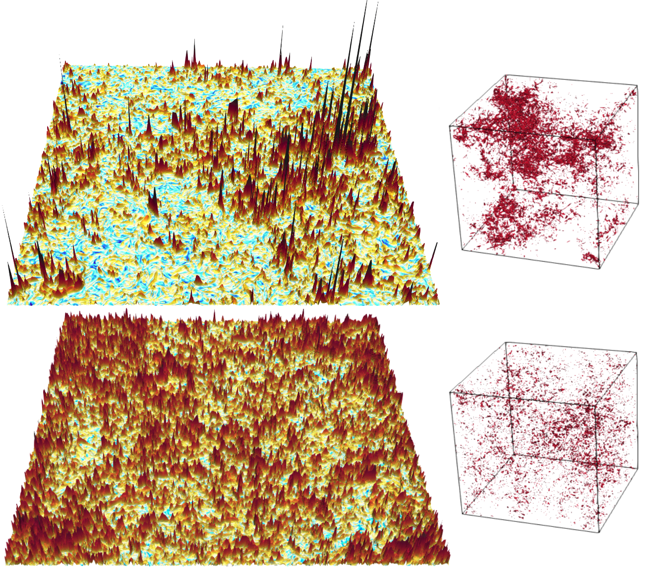
Figure 1: (Top row) Left: visualization of vorticity amplitude in a 2d plane, from a simulation of NSE without control term ($\beta=0$). Right: isocontour regions where the vorticity amplitude is above $20\%$ of its maximum value measured over the flow volume. (Bottom row) Same visualizations obtained from a simulation where the control term is acting on the dynamics of the NSE. Left: visualization of enstrophy plane. Right: contour regions where the vorticity amplitude is above the control forcing threshold fixed at $\omega_{p}=0.2\omega_{max}$. The control forcing amplitude used in the simulation presented here is $\beta=5$. Both simulations are performed with a number of collocation points $N=1024^{3}$.

Method. We consider the Navier Stokes equations (NSE) for an incompressible flow, subjected to two different types of forcing mechanisms:

$$\partial_{t}\,{\boldsymbol{u}}+{\boldsymbol{u}}\cdot{\boldsymbol{\nabla}}{\boldsymbol{u}}=-{\boldsymbol{\nabla}}P+\nu\Delta{\boldsymbol{u}}+{\textbf{F}}-{\boldsymbol{f}}_{c}$$ (1)

where F is a standard large-scale stirring mechanism while ${\boldsymbol{f}}_{c}$ is a second forcing which acts –in our implementation– as a control term on the small-scales dynamics. In particular, in this paper, we will only consider an external smart-drag, proportional to the velocity ${\boldsymbol{f}}_{c}({\boldsymbol{x}},t)=c({\boldsymbol{x}},t){\boldsymbol{u}}({\boldsymbol{x}},t)$ and acting such as to preferentially depleting only those regions where vorticity is important

$$c({\boldsymbol{x}},t)=\beta\,\left(\frac{\text{tanh}\left[(\omega({\boldsymbol{x}},t)-\omega_{p})\right]+1}{2}\right),$$ (2)

where $\omega({\boldsymbol{x}},t)=|{\boldsymbol{\nabla}}\times{\boldsymbol{u}}|$, is the vorticity intensity, $\omega_{p}$ is one threshold above which the control term is strongly active and $\beta$ is an overall rescaling factor of the control amplitude, hence $\beta=0$ would correspond to the usual NSE without control. From its definition it is possible to see that ${\boldsymbol{f}}_{c}({\boldsymbol{x}},t)$ is always close to zero except inside structures dominated by the intense vortex filaments, where the $\tanh$ become positive and equal to 1. The region where ${\boldsymbol{f}}_{c}({\boldsymbol{x}},t)$ is acting can be tuned by changing the threshold $\omega_{p}$, whose value has been fixed as a percentage of the maximum vorticity, $\omega_{max}$, measured in the stationary state of a simulation without the control term, hence:

$$\omega_{p}=p\,\omega_{max}$$

with $0<p\leq 1$. In the transition region around the isoline where $\omega({\boldsymbol{x}},t)=\omega_{p}$ the control function (2) will introduce compressibile effects in (1). Therefore, before adding the control term to (1) one needs to project it on its solenoidal component.

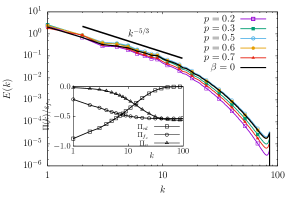
Figure 2: Main panel: energy spectra averaged on time for different simulations at changing the control threshold, $\omega_{c}/\omega_{max}=p$, with a fixed amplitude, $\beta=5$. Notice that $\beta=0$ corresponds to the uncontrooled full NSE. (Inset) Energy fluxes from the non-linear term, $\Pi_{nl}$, from the control term, $\Pi_{f_{c}}$, and from the viscous dissipation, $\Pi_{\nu}$, normalized to the mean energy input, $\varepsilon_{f}$. Here $p=0.2$ and $\beta=5$.

The projection operation breaks the local positive definiteness of the control term, which remains purely dissipative only globally as an average on the whole volume.

Results. In Fig. 1 we present two visualizations of a plane of the vorticity intensity in the stationary state for two simulations, one for the standard NSE (top panel) and one with the control term acting on the flow (bottom panel). The two planes in Fig. 1 are warped upwards depending on the vorticity values, in this way it is possible to see that the intense peaks developed by the NSE are pruned by the small-scales forcing in the controlled dynamics. From the figure it is qualitatively evident that vorticity is strongly depleted when the small-scale drag is acting, as expected. In the same figure, next to the vorticity planes, we show a 3D rendering of the contour regions where the vorticity value is above $20\%$ of its maximum value, for the case of the uncontrolled NSE (top panel) and the contour regions where the vorticity value is above the forcing threshold, $p=0.2$, for the case of the controlled flow (bottom panel). From the volume rendering we can appreciate that the control forcing tends to homogenise the spatial distribution of the intense vorticity events while they result more intermittent and localized when the dynamics is not controlled. It is also interesting to observe that the volume fraction where the forcing is acting is very small even though in those visualizations we are using a broad threshold in terms of the vorticity values, $p=\omega_{p}/\omega_{max}=0.2$.

Energy balance. As already mentioned, the control term has a dissipative global effect on the turbulent dynamics which goes in addition to the normal dissipation produced by the kinematic viscosity. In this way, a second possible channel is opened where the energy, injected by the large scales forcing, can be dissipated. The total energy balance equations becomes:

$$\frac{1}{2}\partial_{t}\langle{\boldsymbol{u}}^{2}\rangle=\nu\langle\Delta{\boldsymbol{u}}^{2}\rangle-\langle{\boldsymbol{f}}_{c}\cdot{\boldsymbol{u}}\rangle+\langle{\boldsymbol{u}}\cdot{\textbf{F}}\rangle.\\$$ (3)

wehere we have the total kinetic energy, $E=\frac{1}{2}\langle{\boldsymbol{u}}^{2}\rangle$, the viscous dissipation $\varepsilon_{{}_{\nu}}=\nu\langle\Delta{\boldsymbol{u}}^{2}\rangle$, the dissipation induced by the control mechanism, $\varepsilon_{c}=\langle{\boldsymbol{f}}_{c}\cdot{\boldsymbol{u}}\rangle$, and the energy injection rate $\varepsilon_{{}_{f}}=\langle{\textbf{F}}\cdot{\boldsymbol{u}}\rangle$, and with $\langle\bullet\rangle$ we intend an average on the whole volume.
Numerical Simulations. To assess the statistical properties of Eq. (1) a set of direct numerical simulation have been performed at changing resolution and the control parameters, namely $\beta$ and $\omega_{p}$. We used a pseudo-spectral code with resolutions up to $1024^{3}$ collocation points in a triply periodic domain $\Omega$ of size $L=2\pi$. Full $2/3$-rule de-aliasing is implemented (see Table I for details). The homogeneous and isotropic external force, F, is defined via a second-order Ornstein-Uhlenbeck process biferale2016coherent . All simulations where control is on, have been produced starting from a stationary configuration of the uncontrolled case $\beta=0$ and all statistical quantities are calculated after that a new stationary state is achieved.

Control	$N$	$\beta$	$p$	$\varepsilon_{f}$	$\nu$
Off	$256$	-	-	2.2	$5.2\times 10^{-3}$
Off	$1024$	-	-	5.5	$8\times 10^{-4}$
On	$256$	$[0.1\div 50]$	$[0.1\div 0.7]$	2.2	$5.2\times 10^{-3}$
On	$1024$	$50$	$[0.05\div 0.6]$	5.5	$8\times 10^{-4}$

Table 1: Parameters used in the simulations. Control: indicates if the control term ($-c({\boldsymbol{x}},t){\boldsymbol{u}}({\boldsymbol{x}},t)$) is applied (On) or not (Off) in Eqs. (1); $N$ is the number of collocation points in each spatial direction; $\beta$ is the amplitude of the control term; $p$ is the percentage of the maximum vorticity above which the control term is active $\omega_{p}=p\omega_{max}$; $\varepsilon_{f}$ is the mean energy input injected by the large scales forcing; $\nu$ is the kinematic viscosity. The amplitude of Ornstein-Uhlenbeck forcing is $f_{0}=0.16$ and $f_{0}=0.14$ for $N=256$ and $N=1024$ respectively; the correlation time is $\tau_{f}=0.6$ for $N=256$ and $\tau_{f}=0.23$ for $N=1024$. The forcing is active on the window $k_{f}=[0.5:1.5]$ for resolution $N=256$ and on $k_{f}=[0.5:2.5]$ for $N=1024$. The Kolmogorovo scale is $\eta=(\nu^{3}/\varepsilon)^{1/4}$, where $\varepsilon$ is the dissipation rate. Resolution is kept at $\eta/dx\geq 0.7$.

In Fig. 2 we present the time average of the instantaneous energy spectra:

$$E(k,t)=0.5\sum_{k<|{\boldsymbol{k}}|<k+1}|{\hat{\boldsymbol{u}}}({\boldsymbol{k}},t)|^{2}$$ (4)

which are almost independent of the control parameter, $p$. Only for the smallest value of $\omega_{p}$, with $p\sim 0.2$, we can notice a small energy depletion at large wavenumbers. However, in all cases, the inertial range scaling properties are unchanged with the slope very close to the Kolmogorov’s prediction $k^{-5/3}$. In the inset of the same figure we show for the controlled simulation with $p=0.2$ and $\beta=5$, the balance of the energy flux produced by the non-linear term, $\Pi_{nl}(k)$, by the viscous drag, $\Pi_{\nu}(k)$ and by the control forcing, $\Pi_{f_{c}}(k)$. In the stationary state we can write the Fourier space energy balance equation as;

$$\Pi_{nl}(k)+\Pi_{f_{c}}(k)+\Pi_{\nu}(k)=\varepsilon_{f}\,,$$ (5)

where $\varepsilon_{f}$ is the large scales energy input of the stochastic forcing. From the inset of Fig. 2 we can see that the control forcing is mainly active in the high wavenumbers where its contribution equals the one from the viscous dissipation, while at small/intermediate wavenumbers the non-linear interactions remain the leading one.

Configuration space statistics. In the following we analyse the statistics of the longitudinal velocity increments defined as $\delta_{r}u=({\boldsymbol{u}}({\boldsymbol{x}}+{\boldsymbol{r}})-{\boldsymbol{u}}({\boldsymbol{x}}))\cdot{\boldsymbol{r}}/r$. In particular we are interested in the assessment of the effects produced by the control term on the intermittent properties of the NSE. To do that we study the scaling properties of the longitudinal structure functions (SF) defined as:

$$S_{p}(r)\equiv\langle[\delta_{r}u]^{p}\rangle\sim r^{\zeta_{p}}.$$ (6)

Intermittency is measured by the departure of the scaling exponents from the Kolmogorov 1941 prediction, $\zeta_{p}=p/3$ in the inertial range, $\eta<r<L_{0}$. In particular, any systematic non-linear dependency on the order of the moment will induce a scale-dependency in the flatness, defined by the dimensionless ratio among fourth and second order SF:

$$F(r)=\frac{S_{4}(r)}{\left[S_{2}(r)\right]^{2}}.$$ (7)

The flatness for the controlled turbulent flow at resolution $N=1024^{3}$ is presented in Fig. 3, for the case with $p=0.2$, compared with the uncontrolled case $\beta=0$ and with the uncontrolled case but with an a-posteriori pruning of all events where $\omega>\omega_{c}$. The latter measurement is introduced in order to understand how much the dynamical pruning imposed by the evolution of eqn. (1) is different from a simple conditioning on small-vorticity events taken on the full uncontrolled NSE. As one can see comparing the empty circles (full $\beta=0$ NSE) with the empty squares (active control with $p=0.2$) the effects on the flatness are dramatic, with both a $100\%$ reduction on the smallest scale and a decrease of the scaling slope in the inertial range. Similarly, by comparing the results with the a-posteriori conditioning (empty triangles) we see that indeed it is crucial to have a dynamical control to deplete intermittency. To our knowledge this is the first evidence that intermittency can be strongly depleted in a dynamical way with a dynamical criterion based on configuration-space filtering, at difference from what obtained by fractal pruning in lanotte15 ; buzz16burg ; lanotte16 ; buzz16lag .

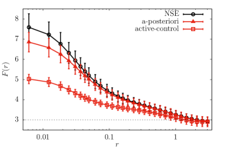
Figure 3: Log-log plot of the flatness, $F(r)$, versus $r$ measured from $30$ different snapshots in time during the evolution of a system with size $N=1024^{3}$. The black lines with open circles (NSE) are data from a simulation without control term ($\beta=0$), while the red line with open squares (active-control) are data from the controlled NSE, using a forcing threshold $\omega_{c}/\omega_{max}=0.2$ and an amplitude $\beta=50$. The black line with full circles (NSE High-Visc) is, again, the NSE without control term but with a higher viscosity value in a way to have the same total drag coefficient, $d_{tot}$, of the controlled simulation. The last curve shown, red line with empty triangles (a-posteriori), is the flatness measured from the same simulation without dynamical control but skipping from the average all regions in the volume where the vorticity module is above the forcing threshold $\omega_{p}/\omega_{max}=0.2$. In all curves, errors are evaluated as the standard deviation from $30$ configurations.

In Fig.  4 we show the effects of the vorticity control point-by-point in the flow volume, by plotting the standardised probability density function (PDF) for the instantaneous and local enstrophy, $|\nabla\times{\boldsymbol{u}}|^{2}$, and shear intensity, ${\cal S}=\sum_{ij}(\partial_{i}u_{j}+\partial_{j}u_{i})^{2}$, for one case of active control, $p=0.2$, and compared with the no-control,$\beta=0$ case. There are two interesting things to remark. First, when the control is active, the far tails of the vorticity are markedly depleted, with almost a sharp cut-off at $\omega\sim\omega_{c}$, which is the clear signature that the control is able to deplete intense vorticity events and to not allow them to grow again during the evolution. This fact is also good news from a sort of min-max approach, it means that the amount of control needed is not too high, being very efficient in stopping the formation of strong vorticity. The second interesting point to remark is that the preferential depletion on vorticity is indeed changing the topological distribution of extreme events in the flow: from the standard case where they are mainly given by high vorticity where no control exist to the case where the extreme fluctuations (far right tails) are more dominated by strong shear events.

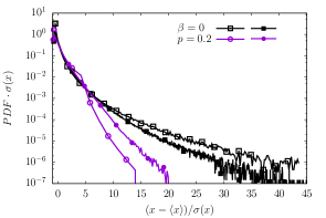
Figure 4: Comparison of the PDFs of enstrophy, $|{\boldsymbol{\nabla}}\times{\boldsymbol{u}}|^{2}$, (open symbols) and shear intensity, ${\cal S}$ (full symbols) measured from simulations of standard NSE (black line) and from the system controlled with forcing threshold, $\omega_{p}/\omega_{max}=0.2$ and amplitude $\beta=5$.

Drag reduction. Going back to the observation of the mean quantities, it is interesting to estimate the effect of the smart forcing on the drag coefficient of the system. Indeed the new smart-control allows the system to preferentially dissipate energy inside the vortical regions where it is active. To quantify its effect we go back to the balance (3) and split the total drag, $d_{tot}$, in two contributions, $d_{\nu}$ and $d_{c}$ as follows:

$$d_{tot}=d_{\nu}+d_{c},\qquad d_{\nu}=\frac{\varepsilon_{\nu}\,\,L_{0}}{u_{rms}^{3}};\qquad d_{c}=\frac{\varepsilon_{c}\,\,L_{0}}{u_{rms}^{3}}$$ (8)

In Fig. 5 we show the mean drag coefficients as a function of the vorticity threshold $\omega_{p}=p\,\,\omega_{max}$ for the simulations with $N=256^{3}$ collocation points and with a moderate control amplitude, $\beta=5$. Fig. 5 shows that the drag contribution coming from the control term is negligible up to a threshold $p\sim 0.6$, instead moving towards lower thresholds the dissipation produced by the small-scales term increases and, around $p=0.2$, the kinematic viscosity and the control dissipations become of the same order. Moving further the threshold towards lower vorticity values the control term becomes the leading contribution responsible for the energy dissipation. In this way, a drag enhancement is observed for the smaller threshold value and the overall drag coefficient is increased almost by a factor $2$ compared to the free NSE at $p=1$.

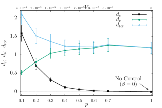
Figure 5: Drag coefficient for the viscous dissipation $d_{\nu}$ (green line), the control forcing $d_{c}$ (black line), and their sum $d_{tot}$ (cyan line). Results are shown as a function of the threshold, $\omega_{p}/\omega_{max}=p$, and the volume fraction, $V$, (upper scale) where the control forcing is acting. Data are measured from simulations with $N=256^{3}$ and a control forcing amplitude $\beta=5$. Errors are evaluated as the standard deviation of the temporal fluctuations observed for the different quantities.

Conclusions. We have presented a first implementation of a smart small-scale control scheme for turbulent flows, based on preferentially damping high vorticity regions. In this study, we have shown that the extra drag exerted on the vortex filaments produce a strong reduction on configuration-based intermittency, with depletion of fat tails and rare events in the vorticity field. The topological relative weight of rotational and extensional regions is also affected abruptly. The overall damping of vortex filaments leads to a sort of drag increase. This study open the way to explore other control Lagrangian mechanism, e.g. based on the heavy-light particles preferential concentration and/or other smart-particles that can be self activated or activated by external control fields, as for the case of magnetic objects. Optimisation of the particles’ properties to track specific flow region can also be attempted in order to enhance/deplete only specific fluctuations reddy16 ; colabrese17flow ; colabrese18smart ; waldock18 ; novati18 .

References

- Frisch (1995) U. Frisch, Turbulence: the legacy of A. N. Kolmogorov (Cambridge University Press, 1995).
- Pope (2001) S. B. Pope, Turbulent flows (IOP Publishing, 2001).
- Benzi et al. (2010) R. Benzi, L. Biferale, R. Fisher, D. Lamb, and F. Toschi, J. Fluid Mech. 653, 221 (2010).
- (4) P.K. Yeung, X.M. Zhai, and K.R. Sreenivasan, PNAS 112.41, 12633-12638 (2017).
- Iyer et al. (2017) K. P. Iyer, K. R. Sreenivasan, and P. K. Yeung, Phys. Rev. E 95, 021101 (2017).
- Sinhuber et al. (2017) M. Sinhuber, G. P. Bewley, and E. Bodenschatz, Phys. Rev. Lett. 119, 134502 (2017).
- (7) J. Bec, L. Biferale, M. Cencini, and A.S. Lanotte, Phys. Rev. Lett. 98(8), 084502 (2007).
- (8) F. Toschi, and E. Bodenschatz, Ann. Rev. Fluid Mech. 41, 375-404 (2009).
- (9) E. Calzavarini, R. Volk, M. Bourgoin, E. Lévêque, J.F. Pinton, and F. Toschi, J. Fluid Mech. 630, 179-189 (2009).
- (10) N.M. Qureshi, U. Arrieta, C. Baudet, A. Cartellier, Y. Gagne, and M. Bourgoin, Eur. Phys. J. B 66(4), 531-536 (2008).
- (11) J.M. Mercado, D.C. Gomez, D. Van Gils, C. Sun, and D. Lohse, J. Fluid Mech. 650, 287-306 (2010).
- (12) M. Gibert, H. Xu, and E. Bodenschatz, J. Fluid Mech. 698, 160-167 (2012).
- (13) K. Gustavsson, and B. Mehlig, J. Fluid Mech. 65(1), 1-57 (2016).
- (14) V. Mathai, E. Calzavarini, J. Brons, C. Sun, and D. Lohse, Phys. Rev. Lett. 117(2), 024501 (2016).
- (15) R. Stanway, Mater. Sci. Tech. 20.8, 931-939 (2004).
- (16) E. Falcon, J.C. Bacri, and C. Laroche, Phys. Rev. F 2.10, 102601 (2017).
- (17) Y. Abe, M. Kawaji, and T. Watanabe, Exp. Therm. Fluid Sci. 26(6-7), 817-826 (2002).
- (18) M. Hauptmann, H. Struyf, S. De Gendt, C. Glorieux, and S. Brems, J. Appl. Phys. 113(18), 184902 (2013).
- (19) M. Hauptmann, H. Struyf, S. De Gendt, C. Glorieux, and S. Brems, ECS J. Solid State Sc. 3(1), N3032-N3040 (2014).
- (20) H.W. Huang, F.E. Uslu, P. Katsamba, E. Lauga, M.S. Sakar, and B.J. Nelson, Scie. Adv. 5(1), eaau1532 (2019).
- (21) J.L. Lumley, J. Polim. Sci.: Macromol. Rev. 7.1, 263-290 (1973).
- (22) C.M. White, and M.G. Mungal, Ann. Rev. Fluid Mech. 40, 235-256 (2008).
- (23) P. Fischer, and A. Ghosh, Nanoscale 3, 557 (2011).
- (24) L. Biferale, F. Bonaccorso, I.M. Mazzitelli, M.A. van Hinsberg, A.S. Lanotte, S. Musacchio, P. Perlekar, and F. Toschi, Phys. Rev. X 6(4), 041036 (2016).
- (25) A.S. Lanotte, R. Benzi, S.K. Malapaka, F. Toschi, and L. Biferale, Phys. Rev. Lett. 115(26), 264502 (2015).
- (26) M. Buzzicotti, L. Biferale, U. Frisch, and S.S. Ray, Phys. Rev. E 93, 033109 (2016).
- (27) A.S. Lanotte, S.K. Malapaka, and L. Biferale, Eur. Phys. J. E 39.4, 49 (2016).
- (28) M. Buzzicotti, A. Bhatnagar, L. Biferale, A.S. Lanotte, and S.S. Ray, New. J. Phys. 18(11), 113047 (2016).
- (29) G. Reddy, A. Celani, T.J. Sejnowski, and M. Vergassola, Proc. Natl. Acad. Sci. U.S.A. 113, E4877 (2016).
- (30) S. Colabrese, K. Gustavsson, A. Celani, and L. Biferale, Phys. Rev. Lett. 118(15), 158004 (2017).
- (31) S. Colabrese, K. Gustavsson, A. Celani, and L. Biferale, Phys. Rev. F 3(8), 084301 (2018).
- (32) A. Waldock, C. Greatwood, F. Salama, and T. Richardson, J. Intell. Robot. Syst. 92(3-4), 685-704 (2018).
- (33) G. Novati, L. Mahadevan, and P. Koumoutsakos, arXiv arXiv:1807.03671, (2018).