Multistability of Driven-Dissipative Quantum Spins

Abstract

We study the dynamics of lattice models of quantum spins one-half, driven by a coherent drive and subject to dissipation. Generically the meanfield limit of these models manifests multistable parameter regions of coexisting steady states with different magnetizations. We introduce an efficient scheme accounting for the corrections to meanfield by correlations at leading order, and benchmark this scheme using high-precision numerics based on matrix-product-operators in one- and two-dimensional lattices. Correlations are shown to wash the meanfield bistability in dimension one, leading to a unique steady state. In dimension two and higher, we find that multistability is again possible, provided the thermodynamic limit of an infinitely large lattice is taken first with respect to the long time limit. Variation of the system parameters results in jumps between the different steady states, each showing a critical slowing down in the convergence of perturbations towards the steady state. Experiments with trapped ions can realize the model and possibly answer open questions in the nonequilibrium many-body dynamics of these quantum systems, beyond the system sizes accessible to present numerics.

Coherent control over quantum single- and few-body dynamics is continuously improving, spanning atomic, optical, and solid-state systems Haroche and Raimond (2006); Yamamoto et al. (2000); Schoelkopf and Girvin (2008). An ongoing effort is focused on assembling many individually tunable systems and studying the ensuing many-body dynamics. A significant challenge lies in realizing unitary dynamics, however, the inevitable presence of dissipative processes can be utilized in different scenarios, such as by reservoir engineering Bardyn et al. (2013). Coherent time-periodic driving is a useful tool Oka and Kitamura (2019), and rich dynamics are observed with systems of strong light-matter interactions at the interface between quantum optics and condensed matter Greentree et al. (2006); Hartmann et al. (2006); Chang et al. (2008); Koch et al. (2010); Petrescu et al. (2012); Cho et al. (2008); Umucalılar and Carusotto (2011); Hafezi et al. (2013); Rechtsman et al. (2013); Otterbach et al. (2013); Carusotto and Ciuti (2013); Le Hur et al. (2016); Noh and Angelakis (2017); Hartmann (2016); Schiró et al. (2016); Fitzpatrick et al. (2017); Fink et al. (2017). Systems with a competition between interactions, nonlinearity, coherent external driving and dissipative dynamics include arrays of coupled circuit quantum electrodynamic units Houck et al. (2012); Schmidt and Koch (2013), cold atoms Bloch et al. (2012), and ions Bohnet et al. (2016). Critical phenomena and dissipative phase transitions in these open systems often come with new properties and novel dynamic universality classes Diehl et al. (2010); Sieberer et al. (2013); Lee et al. (2013); Jin et al. (2013a); Marino and Diehl (2016); Scarlatella et al. (2019); Munoz et al. (2019).

The state of an open quantum system is defined by a density matrix $\rho$, with the dynamics often treated using a Lindblad master equation, describing a memory-less bath, and the time evolution generated by the Liouvillian superoperator acting on $\rho$ Breuer and Petruccione (2002). The theoretical tools available for open quantum many-body systems are relatively limited. For driven-dissipative lattice models the meanfield (MF) approach is often employed, with $\rho$ approximated as a product of single-site density matrices. The dynamics of local observables are described by nonlinear equations, studied, e.g., for lattice Rydberg atoms Lee et al. (2011); Qian et al. (2012); Marcuzzi et al. (2014); Carr et al. (2013); Letscher et al. (2017); Parmee and Cooper (2018), coupled quantum-electrodynamics cavities and circuits Jin et al. (2013b, 2014); Schiró et al. (2016), nonlinear photonic models Foss-Feig et al. (2017); Biondi et al. (2017a), and spin lattices Chan et al. (2015); Wilson et al. (2016). A key feature of the MF phase diagrams are multistable parameter regions where two or more steady states coexist.

However, the Lindblad equation converges in general to a unique steady state in finite systems Spohn (1977); Minganti et al. (2018), making the status of the MF approximation unclear. Indeed, significant deviations from MF have been found using approximation schemes accounting for quantum correlations Weimer (2015); Biondi et al. (2017b); Jin et al. (2016), and also using exact numerical methods (quantum trajectories Daley (2014) and Matrix Product Operators (MPO) Prosen and Žnidarič (2009)). In one-dimensional (1D) lattices with nearest-neighbour (NN) interactions, the MF bistability is found to be replaced by a crossover driven by large quantum fluctuations Weimer (2015); Mendoza-Arenas et al. (2016); Foss-Feig et al. (2017); Vicentini et al. (2018). In contrast, in certain 2D NN models, MF bistability has been found by approximate methods to be replaced by a first-order phase transition between two states, for nonlinear bosons using a truncated Wigner approximation Foss-Feig et al. (2017); Vicentini et al. (2018), and for Ising spins using a variational ansatz acounting for short-range correlations Weimer (2015), a cluster MF approach Jin et al. (2018) and two-dimensional tensor network states Kshetrimayum et al. (2017). In a parameter region around the jump, the convergence towards the steady state slows down Weimer (2015); Vicentini et al. (2018), a phenomenon related to a gap closing in the spectrum of the Liouvillian Cai and Barthel (2013); Macieszczak et al. (2016); Minganti et al. (2018).

In this Letter we study a driven-dissipative model of spins one-half with XY (flip-flop) interactions in presence of coherent drive and dissipation, using a combination of MPO simulations and an approximation scheme which accounts for quantum fluctuations beyond meanfield (MFQF). For one dimensional lattices we confirm the existence of a unique steady state in the thermodynamic limit. As our main result, we find that in dimension two and higher multistability (in particular, bistability) is again possible, with jumps between the different steady states accompanied by a critical slowing down, provided that the thermodynamic limit of an infinitely large lattice is taken first with respect to the long time limit. We argue that this order of limits is physically plausible, and we link the bistability to the fact that for finite size and time the probability distribution of relevant observables develops a strong bimodal structure. Depending on the order of limits, bimodality leads either to a first-order dissipative phase transition (as usually discussed when the long time limit is taken first), or to a bistable regime. We thus provide a theoretical scenario reconciling our results with the literature cited above, and finding similar dynamics in a model with Ising interactions (see below and App. B) indicates the generality of our results. We suggest that in an experimental platform based on trapped-ion quantum simulators, such a question can be addressed.

Model. We consider a quantum system with $N$ sites $R\in\mathbb{Z}^{D}$ on a hypercubic lattice in $D$ spatial dimensions, for which the connectivity is $\mathcal{Z}=2D$. The master equation for $\rho$ is defined using the Liouvillian $\hat{\mathcal{L}}$,

$$\partial_{t}\rho=\hat{\mathcal{L}}[\rho]\equiv-i[H,\rho]+\mathcal{D}[\rho],\qquad\hbar=1.$$ (1)

The Hamiltonian describing Rabi oscillations of two-level systems with a drive detuned by $\Delta$ from the resonant transition frequency and a Rabi frequency $\Omega$, is given in a frame rotating with the drive by

$$H=\sum_{R}\left[\frac{\Delta}{2}\sigma_{R}^{z}+\Omega\sigma_{R}^{x}\right]-\sum_{\langle R,R^{\prime}\rangle}J\left(\sigma^{+}_{R}\sigma^{-}_{R^{\prime}}+{\rm h.c.}\right),$$ (2)

where the second sum extends over all pairs of NN sites, describing hopping with amplitude $J$, with spin-$\frac{1}{2}$ operators (Pauli matrices) $\sigma_{R}^{a}$, $a=\{x,y,z\}$, and $\sigma^{\pm}_{R}=({\sigma^{x}_{R}\pm i\sigma^{y}_{R}})/{2}$. For spin losses occurring independently at each site with rate $\Gamma=1$ (which fixes the frequency and time units),

$$\mathcal{D}[\rho]=\sum_{R}\left[\sigma_{R}^{-}\rho\sigma_{R}^{+}-\frac{1}{2}\left(\sigma_{R}^{+}\sigma_{R}^{-}\rho+\rho\sigma_{R}^{+}\sigma_{R}^{-}\right)\right].$$ (3)

Aside from translation invariance, this model has no manifest microscopic symmetries. Its MF phase diagram displays bistability Mendoza-Arenas et al. (2016); Wilson et al. (2016) in a region of parameters that terminates at a second order point where an emerging $Z_{2}$ symmetry spontaneously breaks Marcuzzi et al. (2014). In 1D the steady state is unique as obtained by MPO simulations Mendoza-Arenas et al. (2016). Here we focus on higher dimensions, which we find to manifest bistability in the thermodynamic limit.

Dynamics of Observables. From the master equation one can derive a hierarchy of equations of motion for $n$-points expectation values of the form $\langle\sigma_{R_{1}}^{a}\sigma_{R_{2}}^{b}\cdots\sigma_{R_{n}}^{c}\rangle\equiv{\rm tr}\{\rho\sigma_{R_{1}}^{a}\sigma_{R_{2}}^{b}\cdots\sigma_{R_{n}}^{c}\}$, which depend on the value of correlators at the next order, $n+1$. Assuming a translationally-invariant density matrix, we define the uniform vector mean magnetization, $\mu_{a}(t)=\left\langle\frac{1}{N}\sum_{R}\sigma_{R}^{a}\right\rangle=\left\langle\sigma_{R}^{a}\right\rangle$, and its equations of motion

$$\partial_{t}\mu_{x} = -{J}\mathcal{Z}[\mu_{y}\mu_{z}+\eta_{yz}(1)]-{\Delta}\mu_{y}-\mu_{x}/2,\quad$$ (4)

$$\partial_{t}\mu_{y} = {J}\mathcal{Z}[\mu_{x}\mu_{z}+\eta_{xz}(1)]-2\Omega\mu_{z}+{\Delta}\mu_{x}-\mu_{y}/2,\quad$$ (5)

$$\partial_{t}\mu_{z} = 2\Omega\mu_{y}-\left(1+\mu_{z}\right).\quad$$ (6)

with the connected two-point correlation functions,

$${\eta}_{ab}(R,R^{\prime},t)\equiv\left\langle\left(\sigma_{R}^{a}-\mu_{a}\right)\left(\sigma_{R^{\prime}}^{b}-\mu_{b}\right)\right\rangle\\ =\left\langle\sigma_{R}^{a}\sigma_{R^{\prime}}^{b}\right\rangle-\mu_{a}\mu_{b},\quad R\neq R^{\prime},$$ (7)

and setting $R^{\prime}=0$ using the translation invariance, ${\eta}_{ab}(1)$ is the correlator at a NN of the origin.

Equations (4)-(6) are exact. The limit ${\eta}\to 0$ reduces $\rho$ to a product of identical on-site states, leading to the MF equations, whose steady state and dynamics are studied in detail in Landa et al. . We present an approximate scheme going beyond MF, formally based on an expansion in $1/\mathcal{Z}$ (with a related approach in Biondi et al. (2017b)). Neglecting the connected three-point correlators $\left\langle\left(\sigma_{R}^{a}-\mu_{a}\right)\left(\sigma_{R^{\prime}}^{b}-\mu_{b}\right)\left(\sigma_{R^{\prime\prime}}^{c}-\mu_{c}\right)\right\rangle\approx 0$, allows us to derive (see App. E) coupled equations for $\eta_{ab}(R,t)$, which we solve numerically together with their feedback into Eqs. (4)-(6). Since the short-range correlators $\eta_{ab}(1)$ appearing in Eqs. (4)-(6) are dynamically coupled to all distances in the lattice, the MFQF method accounts for the spatial structure of correlation functions. The simulations have been verified to converge as a function of $N$, and hence we can approximate the system dynamics as a function of time with the limit $N\to\infty$ taken first.

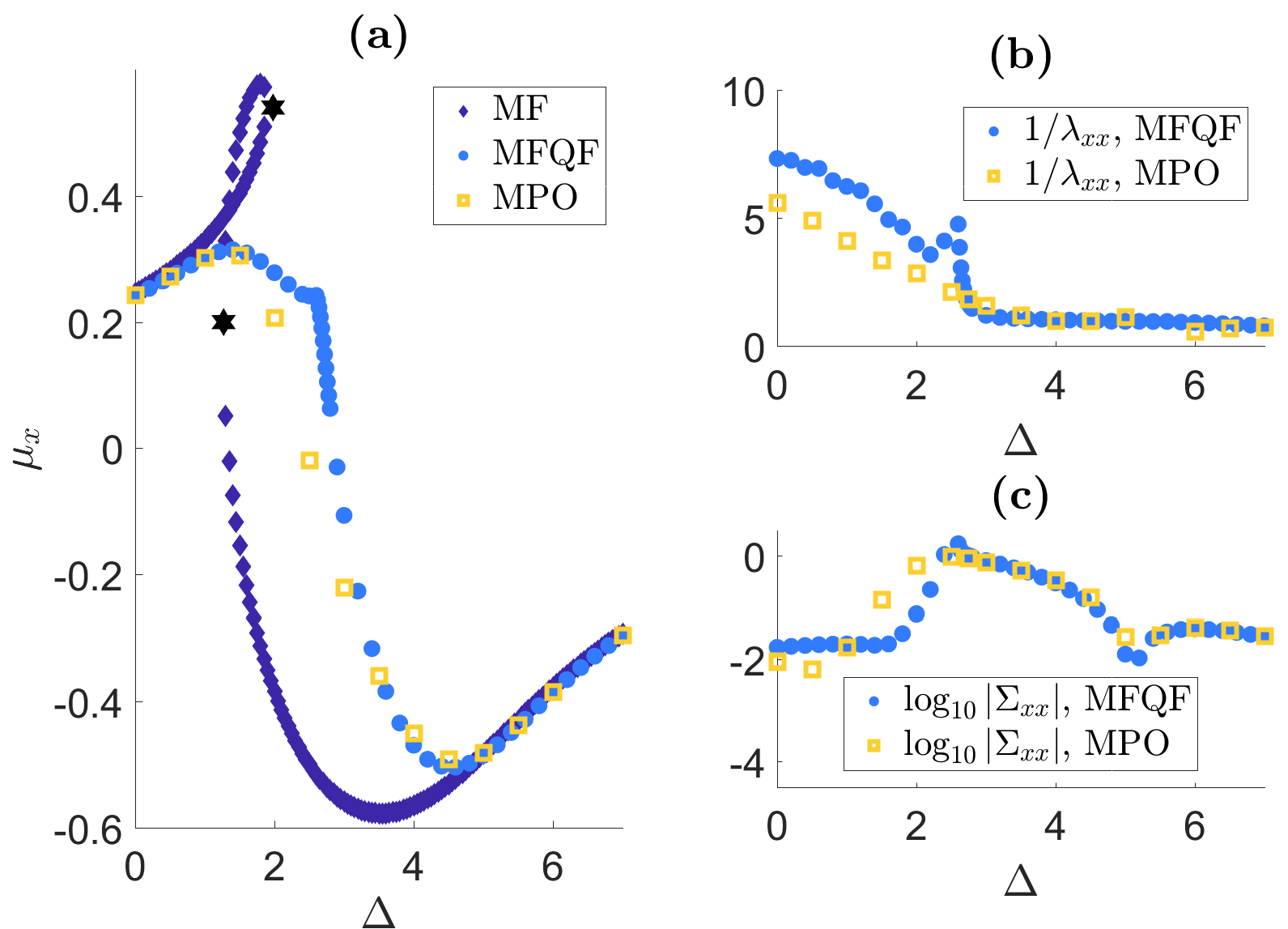
Figure 1: (a) Mean steady-state $x$ magnetization $\mu_{x}^{S}$ as a function of $\Delta$ for $\Omega=0.5$ and $J\mathcal{Z}=4$, on a 1D lattice. The meanfield (MF) limit manifests bistability, with three co-existing solutions, two of which – those on the branches coming from the limits of $\Delta\to\{0,\infty\}$, are stable. Two black hexagrams mark the points where the unstable branch meets each of the two stable ones. An exact numerical treatment using Matrix Product Operators (MPO) shows a crossover within a range of $\Delta$ shifted from the MF bistability region. An approximation incorporating quantum fluctuations at leading order (MFQF) follows approximately the MPO result in a large range of parameters. (b) The correlation length $\lambda_{xx}$ defined by fitting $\eta_{xx}\sim\exp\{-\lambda_{xx}R\}$, and (c) the total correlation $\Sigma_{xx}=\sum_{R}\eta_{xx}(R)$, calculated in MPO and MFQF, showing that the latter approximation is capable of capturing the spatial structure and relative magnitudes of two-point correlations in the lattice.

Correlations wash away Bistability in 1D. We start our analysis with numerically exact MPO calculations of large lattices in 1D. The density matrix $\rho$ can be considered as a pure state in an enlarged Hilbert space with four states per site Mascarenhas et al. (2015), allowing us to solve the Lindblad evolution using a method formally similar to pure state unitary evolution encoded using well-established matrix product states (see Schollwöck (2011); Zaletel et al. (2015) and references therein). We evolve $\rho(t)$ in a 1D chain with open BC (translation invariance is not enforced), using an MPO algorithm Prosen and Žnidarič (2009); Benenti et al. (2009); Mascarenhas et al. (2015), with an implementation based on the iTensor library ite (n 21), a Trotter decomposition of order four Zaletel et al. (2015); Bidzhiev and Misguich (2017), and bond dimension $\chi=300$. With up to 200 spins we checked that observables measured in the central region of the chain had negligible finite-size effects and truncation errors at the scale of the plots, allowing us to obtain their steady-state bulk values corresponding to the thermodynamic limit.

Figure 1(a) shows the $x$ component of the steady-state magnetization, $\vec{\mu}^{S}\equiv\lim_{t\to\infty}\vec{\mu}(t)$, in 1D, for $J\mathcal{Z}=4$ as a function of $\Delta$. In MF, $\vec{\mu}^{S}$ is unique except for $1.3\lesssim\Delta\lesssim 1.9$, where there are two co-existing stable solutions in addition to an unstable solution. At the presence of quantum correlations (in MPO and MFQF), the magnetization departs significantly from the MF prediction, with a crossover between the two limiting regimes, in the range $1.5\lesssim\Delta\lesssim 5$. We define the inverse correlation lengths $\lambda_{ab}$ by fitting the six correlation functions to $\eta_{ab}(R)\sim\exp\{-\lambda_{ab}R\}$. For simplicity, we present in Fig. 1(b) only one correlation length, and Fig. 1(c) shows the corresponding total correlation measured by $\Sigma_{ab}=\sum_{R}\eta_{ab}(R)$. The spatial structure of the two-point correlation undergoes a sharp change within the crossover region, from relatively small but widely extended correlations for low $\Delta$, to much larger but very short-ranged correlations, for high $\Delta$. A separate analysis of the correlations shows that at the same time, the correlations change nature from periodic modulations (spin density-wave character), to being overdamped in space.

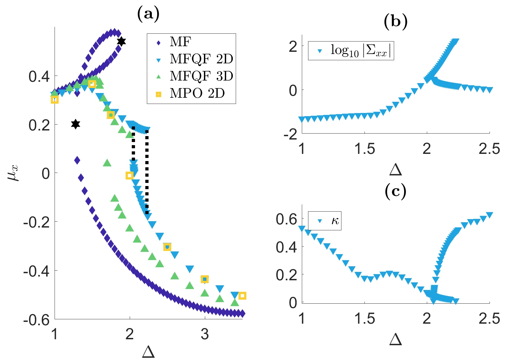
Figure 2: (a) Mean steady-state $x$ magnetization $\mu_{x}^{S}$ in the MFQF $N\to\infty$ approximation in 2D-3D, together with the MF limit and 2D-MPO results (for a $12\times 4$ cylinder). The parameters are as in Fig. 1, with ${J}\mathcal{Z}$ kept fixed by varying $J$ with the dimension. For $D\geq 2$ MFQF predicts multistability, with two stable branches approaching the MF branches in an increasingly larger parameter region as $D$ is increased. The dotted black lines indicate the edges of the 2D bistable region. The simulations were run with lattices of up to $200^{2}$ and $40^{3}$ sites and periodic BC. (b) The total correlation in 2D, showing a difference of up to two orders of magnitude in the bistable phases. (c) The rate of convergence to the 2D steady states, fitted to an exponential form $\sim e^{-\kappa t}$, showing a critical slowing down of the dynamics as $\kappa\to 0$ at the two bistability edges.

As Fig. 1 shows, the MFQF approximation correctly captures the uniqueness of the steady state and the disappearance of bistability in 1D. On both sides of the crossover region, the results are quantitatively accurate. In its center, the approximation reaches too large values for $\eta_{ab}(R)$ and the correlation length. More generally, we find that as $J$ is increased in 1D, the MFQF approach loses its accuracy (for parameters of strong correlations), plausibly because of the role of higher-order correlation functions that are neglected, which can lead at much larger $J$ to the breakdown of the approximation. However, the MFQF approach is easy to generalize to higher dimensions, and quantitatively accurate in regions with moderate correlations.

Bistability in Higher dimensions. Figure 2(a) shows the results of simulations with large 2D and 3D lattices, for $J\mathcal{Z}=4$. The MFQF theory, that allows simulating large lattices (with $N\to\infty$), is compared with 2D-MPO calculations, limited to a finite-size system, for which, as in 1D, $\rho$ is encoded as a product of matrices. The matrix product runs over a snake-like path visiting all the sites of a cylinder of length $L_{x}=12$ and perimeter $L_{y}=4$ (see App. C). Such an approach has been applied in ground-state calculations of 2D models Stoudenmire and White (2012), but we are not aware of previous 2D-MPO Lindblad calculations. For $\Delta\lesssim 1.5$ and $\Delta\gtrsim 2.5$ the agreement between MPO and MFQF is almost perfect, giving a nontrivial check of the ability of MFQF to capture significant correlation effects (that result in $\vec{\mu}$ strongly departing from MF). The computational cost of guaranteeing a high accuracy in 2D-MPO calculation is exponential in $L_{y}$ (see App. C), limiting the present MPO calculations to relatively small systems, which cannot show bistability (and a possible discontinuity would also be smeared out).

As our main result, using MFQF we find in 2D two stable $\vec{\mu}^{S}$ branches, that in 3D extend over larger ranges of $\Delta$, converging towards the MF bistability region and magnetization values. Figure 2(b) shows that $\Sigma_{xx}$ increases by two orders of magnitude for one of the bistable states, and Fig. 2(c) shows the asymptotic relaxation rate associated to the convergence to $\vec{\mu}^{S}$. It is obtained by fitting $\partial_{t}\vec{\mu}^{2}\sim e^{-\kappa t}$ at large times ($t\sim 100$). The fact that $\kappa\to 0$ at the branch edges in 2D indicates a critical slowing down when approaching the end of the bistability region in the phase that is about to disappear, leading to a discontinuous jump. The MFQF approach does however not always predict bistability in 2D. Replacing each hopping term in Eq. (2) by the Ising coupling $J_{z}\sigma_{R}^{z}\sigma_{R^{\prime}}^{z}$, we find a smooth crossover for moderate $J_{z}$ (as obtained using cluster meanfield Jin et al. (2018)), and a small bistability region for stronger couplings (again as in Jin et al. (2018)); See App. B.

Bistability, Liouvillian spectrum and bimodality. We henceforth return to the question raised in the introduction: how to reconcile the uniqueness of the steady state in finite systems, with bistability seen when taking first the thermodynamic limit of infinite size, and then the long-time limit?

Considering the Liouvillian $\hat{\mathcal{L}}$ of Eq. (1), the unique thermodynamic steady state corresponds to $\rho_{ss}=\lim_{N\to\infty}\lim_{t\to\infty}\rho(t)$, which is independent of the initial conditions, and is an eigenstate of $\hat{\mathcal{L}}$ at any $N$, $\hat{\mathcal{L}}\rho_{ss}=0$. Assuming bistability, we define $\rho_{1}$ and $\rho_{2}$ as the two distinct density matrices obtained from $\lim_{t\to\infty}\lim_{N\to\infty}\rho(t)$, which depend on the initial conditions. For $N$ large but finite the bistability should be replaced by long-lived metastable states, in which case $\rho_{1}$ and $\rho_{2}$ are defined at times $t\gg 1/\Gamma$, but small compared to the lifetime of these metastable states. As in the model studied here, these two states have different local properties: a local observable (i.e. sum of local terms, e.g. $M_{x}=\frac{1}{N}\sum_{R}\sigma^{x}_{R}$) has a probability distribution $P_{1}(m)$ with a single peak centred around $m_{1}$ in $\rho_{1}$, and a distribution $P_{2}(m)$ peaked around $m_{2}$($\neq m_{1}$) in $\rho_{2}$. At the same time, metastability implies some relaxation time diverging with $N$, and the spectrum of $\hat{\mathcal{L}}$ must have at least one nonzero eigenvalue $\lambda_{E}$ with a vanishingly small real part, $\lim_{N\to\infty}{\rm Re}(\lambda_{E})=0$, other eigenvalues being separated by a gap $\mathcal{O}(\Gamma)$ Macieszczak et al. (2016); Rose et al. (2016). We assume for simplicity that $\hat{\mathcal{L}}$ has a unique such small eigenvalue (therefore real), and denote by $\rho_{E}$ the associated eigenstate (or eigenmatrix). $\rho_{ss}$ and $\rho_{E}$ are the eigenstates from which all long-lived states can be constructed, since for $t$ much larger than $1/\Gamma$ we can ignore higher “excited” eigenstates. So, for $\rho_{1}$ and $\rho_{2}$ to be long-lived, they must be linear combinations of $\rho_{ss}$ and $\rho_{E}$. As physical states have a trace equal to 1, and since ${\rm Tr}\rho_{ss}=1$ and ${\rm Tr}\rho_{E}=0$, there must exist two distinct scalars $a_{1}$ and $a_{2}$ such that $\rho_{i}=\rho_{ss}+a_{i}\rho_{E}$ with $i=1,2$ Macieszczak et al. (2016); Rose et al. (2016); Minganti et al. (2018); Letscher et al. (2017). Inverting these relations we get $\rho_{ss}=(a_{2}\rho_{1}-a_{1}\rho_{2})/(a_{2}-a_{1})$. So, if $a_{1}$ and $a_{2}$ are both nonzero (which may not be always the case) $\rho_{ss}$ is a “cat state” (with correlation functions extending over the system size), being a linear combination of two uniform physical states with different local properties. In $\rho_{ss}$, the probability distribution $P_{\rm ss}=(a_{2}P_{1}-a_{1}P_{2})/(a_{2}-a_{1})$ of a local observable is bimodal, peaked around the two mean values $m_{1,2}$ realized in the states $\rho_{i=1,2}$.

Using exact diagonalization on small systems we have computed such distributions for the fully-connected (FC) version of the present XY model, which is bistable in the thermodynamic limit (where MF becomes exact), and for the 1D and 2D cases. We find (App. A), that the magnetization becomes bimodal in parts of the MF bistability region for the FC and 2D cases, whereas it stays mono-modal in 1D. The scaling with $N$ of the bimodal peaks is beyond the scope of the current work, however, the mean value of an observable computed with $\rho_{ss}$ may become discontinuous as $N\to\infty$ at some value of the parameter Foss-Feig et al. (2017); Casteels et al. (2017); Vicentini et al. (2018); Minganti et al. (2018). This could correspond, in the discussion above, to smoothly varying $\rho_{i=1,2}$ but discontinuous jumps of $a_{1}$ and $a_{2}$. Hence, a unique steady state with a discontinuous jump is a-priori compatible with bistability and hysteresis and, in the present scenario, finding one or the other in a theory calculation is a matter of order of limits.

Moreover, since the support of $P_{1}$ has essentially no overlap with that of $P_{2}$ (for a large enough system), any density matrix which is not a convex combination of $\rho_{1}$ and $\rho_{2}$ would give some (unphysical) negative probability density. This means that all physical long-lived states are convex combinations of the mono-modal states $\rho_{i}$, and the latter thus coincide with the extreme states of Macieszczak et al. (2016). The above discussion therefore connects our results both with the theories of first-order phase transitions, and the theory based on the extreme metastable states. The lifetimes of the many-body metastable states would diverge with $N$, plausibly $\propto e^{N}$, and for large enough $N$, exceed the time accessible in numerical or experimental realizations. We conjecture that an initial state with a finite correlation length will lead, in the time window $1/\Gamma\ll t\ll 1/|\lambda_{E}|$, to one of the two mono-modal states $\rho_{i}$, and not to an arbitrary combination of the two. A heuristic argument is given in App. D. A product state is a natural reproducible initial state in an experiment, allowing to explore the metastability. As a parameter is swept back and forth across the bistability region in an experimental setup, observables will show hysteretis loops – unless the sweep is unrealistically slow ($\propto e^{-N}$).

Experimental feasibility. In addition to possible realizations with circuit-QED arrays Mendoza-Arenas et al. (2016), driven-dissipative spin models can be realized in current experiments with a few tens to a few hundreds of trapped ions. Ising and XY interactions can be implemented by laser beams inducing spin-motion coupling along one or two orthogonal directions Porras and Cirac (2004); Friedenauer et al. (2008); Schneider et al. (2012), with an additional laser for the on-site Hamiltonian. As recently demonstrated experimentally, the interaction can be varied from being almost independent of distance to a dipolar power-law, and therefore short-range in 1D Islam et al. (2013); Smith et al. (2016) and 2D lattices Bohnet et al. (2016). The interaction strength in these works is of order $J/\hbar\sim 10^{4}s^{-1}$, one to two orders of magnitude larger than the qubit dephasing rates, and the rate of spin-flip processes in Eq. (3) can be potentially controlled as well.

To conclude, studying lattices of driven-dissipative interacting spins using state-of-the-art 1D MPO simulations, for the parameters presented here and in further parameter regimes Landa et al. , we have found no phase transition but a crossover between two regimes with different characteristics. On the other hand, using a new approach that accounts for the leading-order lattice correlations and their feedback onto the mean magnetization, bistability appears to be possible in driven-dissipative quantum systems already in 2D. Thus, the present exact and approximate calculations suggest that $D=2$ is a lower critical dimension for bistability in this problem. This conclusion is consistent with works done in the context of Rydberg atoms on related models Marcuzzi et al. (2014), pointing toward a model-A dynamic universality class (whose lower critical dimension is known to be two) for the second order phase transition at the ending point of the bistability regime. This implies that in one dimension fluctuations destroy the critical point and with it the entire bistability region, in line with our results.

The question of the existence of a lower critical dimension for bistability, bimodality and hysteresis and the accompanied dissipative phase transitions in this model can be directly addressed experimentally. If a definite answer is found, it would constitute the first demonstration of deciding a question currently intractable classically, by a controlled quantum simulation. It could ascertain the status of the meanfield approximation in these systems, and shed light on the differences between equilibrium and nonequilibrium phase transitions.

Appendix A Bimodality

We start studying the model of Eqs.(1)-(3) of the main text on a finite FC lattice with $N$ sites, i.e. a graph where all sites are linked (with connectivity $\mathcal{Z}=N-1$). The FC version of the model is interesting because: (i) it has a unique steady state for any finite $N$, (ii) its meanfield (MF) solution gives a set of non-linear differential equations which can support bistability, and (iii) the MF approximation becomes asymptotically exact in the limit $N\to\infty$. This is due to the fact that each site is coupled to the $x$ and $y$ components of the total magnetization of the $N-1$ other sites, and the fluctuations of this magnetization generically become small compared to its mean when $N\to\infty$. As the thermodynamic limit $N\to\infty$ is approached, the bistability is thus expected to appear in some way and the FC model can be viewed as a playground to investigate how a unique steady state at finite $N$ can be reconciled with bistability in the thermodynamic limit.

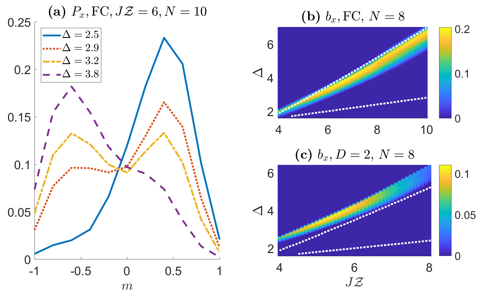
Figure 3: (a) Probability distribution $P_{x}=P(M_{x}=m)$ of the $x$ magnetization per-site ($M_{x}=\frac{1}{N}\sum_{R}\sigma^{x}_{R}$), for a few values of the detuning $\Delta$, at fixed $J\mathcal{Z}$ and $\Omega=0.5$, in the steady state of the XY model with $N=10$ spins on a fully connected (FC) lattice. The transition from a single peak centered at $m>0$ to a single peak at $m<0$ as $\Delta$ is increased, is accompanied by an intermediate region of a bimodal distribution. (b) The bimodality index $b_{x}$ (see text) given by the color code, with $\Omega=0.5$ and $N=8$ for the FC lattice. Within the region bounded by the two white dotted lines, the meanfield limit manifests bistability of two different steady-state magnetizations. (c) $b_{x}$ for a two-dimensional ($2D$) parallelogram of $N=8$ sites and periodic boundary conditions (note the smaller $J\mathcal{Z}$ range). We find bimodality, although weaker than in the FC model, and with stronger finite-size effects.

We thus compute exactly the unique stationary state density matrix $\rho_{ss}=\lim_{t\to\infty}\rho(t)$ on small systems. We focus on the probability distribution of the $x$ magnetization per site, i.e. $P_{x}=P(M_{x}=m)$, where $M_{x}=\frac{1}{N}\sum_{R}\sigma_{R}^{x}$, that we plot in Fig. 3(a) at fixed $\Omega$ and $J\mathcal{Z}$ (the rescaling by $\mathcal{Z}$ allows to compare lattices of a different connectivity), and for different values of $\Delta$. Quite interestingly, such probability distribution evolves from a single peak centered around $m>0$ to a single peak centered around $m<0$, with an intermediate $\Delta$ range where $P_{x}$ has two separated peaks. To quantify the bimodality of the distribution we define an index $b_{x}=2(P_{\max,2}-P_{\min})/(P_{\max,1}+P_{\max,2})$, where $P_{\max,2}\leq P_{\max,1}$ are the two maxima of the distribution, and $P_{\min}$ is the minimum between the two. As can be seen in Fig. 3(b), the extent of the bimodality region in $\Delta$ and the maximum of $b_{x}$ increase with $J\mathcal{Z}$ at a fixed $\Omega$, following the MF bistability region.

While in the finite size limit we consider here the stationary state is still unique and the average value of the observable will either evolve smoothly with $\Delta$ or give rise to a step, depending on the scaling with $N$ of the peaks, the emergence of a bimodal probability distribution suggests a possible scenario for bistability to survive. Indeed for a FC lattice taking the thermodynamic limit first leads to a set of non-linear differential equations which can support multiple stable solutions. This should translate, in the probability distribution of the magnetization at finite size and finite time, and depending on the initial condition, in the emergence of a second peak on time scales exponentially in the system size such that, in the thermodynamic limit the switching from one solution to the other becomes exponentially suppressed.

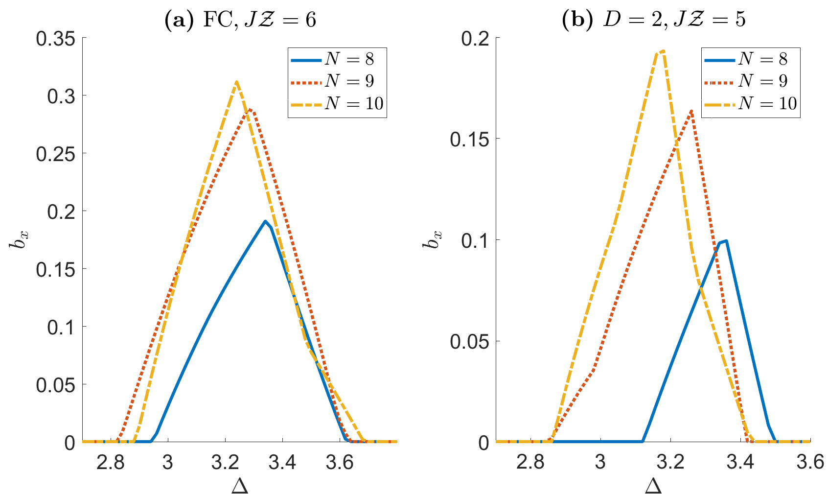
Figure 4: The bimodality index $b_{x}$ (see text) as a function of $\Delta$ for (a) $J\mathcal{Z}=6$ in a fully-connected (FC) lattice, and (b) $J\mathcal{Z}=5$ in a 2D lattice, from exact numerical solutions of the master equation of the driven-dissipative XY model, for small lattices, with three values of $N=8,9,10$.

Repeating this analysis for a 2D square lattice with periodic boundary conditions (BC) we find again a bimodal parameter region, shifted towards higher $\Delta$, with and the maximum $b_{x}$ smaller than in the FC model [Fig. 3(c)]. With an increasing interaction strength $J$, the magnitude and extent of correlated fluctuations in the lattice grow, explaining the gradual decrease of the bimodal parameter region for a small lattice. As further consistency checks, we verified that when increasing $N$ (up to 10) at specific parameter values, the bimodality range and maximum increase, and for a 1D chain we find (not shown) that $b_{x}$ remains strictly zero.

Figure 4 shows the bimodality index $b_{x}$ calculated exactly for three increasing lattice sizes (in the 2D case shown in panel (b), different parallelograms are constructed with periodic boundary conditions to incorporate $N$ sites), for the driven-dissipative XY model discussed in the main main text. Although sensitive to the finite system size, the width of the $\Delta$ ranges of bimodality increase with $N$ and the maximal $b_{x}$ value increases accordingly, which is consistent with bistability in the $N\to\infty$ limit.

Appendix B Bistability in a driven-dissipative Ising model in 2D

We have employed the MFQF method to the study of the driven dissipative Ising model, obtained after replacing the XY (flip-flop) interaction term in the Hamiltonian,

$$H=\sum_{R}\left[\frac{\Delta}{2}\sigma_{R}^{z}+\Omega\sigma_{R}^{x}\right]-\sum_{\langle R,R^{\prime}\rangle}\frac{J_{z}}{2}\sigma^{z}_{R}\sigma^{z}_{R^{\prime}},$$ (8)

while keeping the dissipator identical. The equations of motion for $\vec{\mu}$ that are obtained from this model are identical to those in Eqs. (4)-(6) of the main text with just the replacement $J\to-J_{z}$. The correlator equations (given in the following), are different.

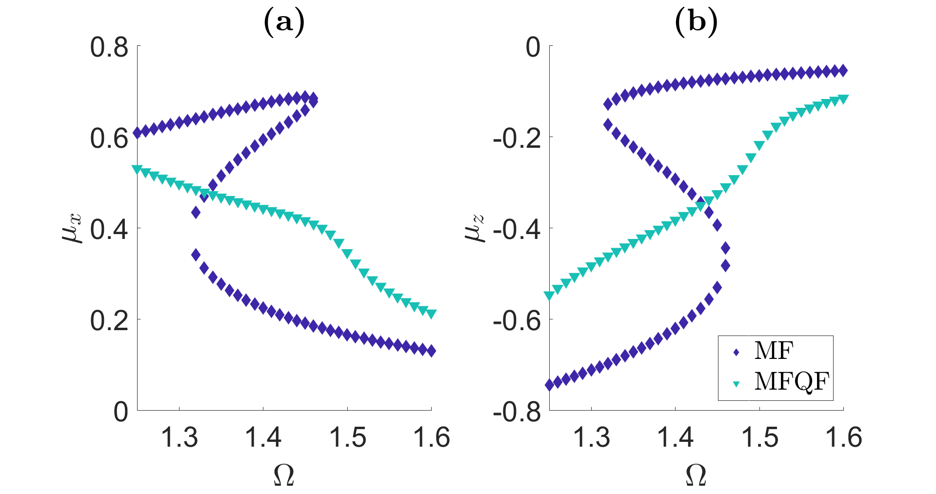
Figure 5: (a) Mean steady-state $x$ magnetization $\mu_{x}^{S}$ as a function of $\Omega$ for $\Delta=0$ and $J_{z}\mathcal{Z}=-4$, on a 2D lattice for the Ising model. (b) The mean steady-state $z$ magnetization for the same parameters. The MF manifests bistability in the $\Omega$ range shown, while MFQF predicts a smooth crossover. We note that in the notation of Ref. Jin et al. (2018), $\Omega=(h_{x}/\gamma)/2$, and $J_{z}\mathcal{Z}=-V/\gamma$ and the current figure corresponds to Fig. 1(a) of Ref. Jin et al. (2018), in a somewhat larger $\Omega$ range, showing a rather sharp change around $\Omega\approx 1.5$. The simulation accounts for a lattice of $100^{2}$ sites, and the results have been verified to converge in $N$ and $t$.

Setting $\Delta=0$ we have studied the resulting MFQF steady state on a 2D lattice. A necessary condition for bistability in the meanfield limit Landa et al. , is $|J_{z}\mathcal{Z}|>2$. For $J_{z}\mathcal{Z}=-4$, Fig. 5 shows a smooth crossover of the steady-state magnetization $\vec{\mu}^{S}$ as a function of $\Omega$ across the parameter region of meanfield bistability. The $z$ magnetization curve of Fig. 5(b) can be compared with the results plotted in Fig. 1(a) of Jin et al. (2018), which were obtained using a cluster MF approach for different cluster sizes. In the notation of Ref. Jin et al. (2018), $J_{z}\mathcal{Z}=-V/\gamma$ and $\Omega=(h_{x}/\gamma)/2$, making the parameters in the plots identical (with only a somewhat larger range taken here for the abscissa). The MFQF curve that we obtain contains a further noticeable feature around $\Omega\approx 1.5$, with a relatively sharper change in magnetization.

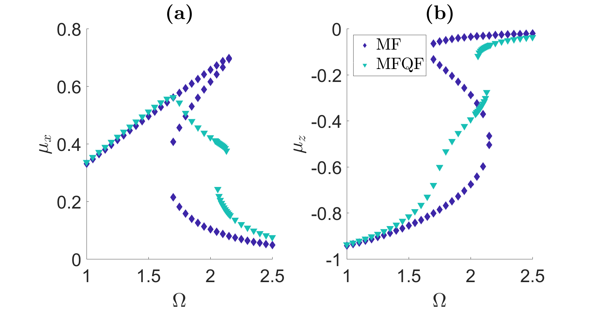
Figure 6: (a) Mean steady-state $x$ magnetization $\mu_{x}^{S}$ as a function of $\Omega$ for $\Delta=0$ and $J_{z}\mathcal{Z}=-6$, on a 2D lattice for the Ising model. (b) The mean steady-state $z$ magnetization for the same parameters. The MF manifests bistability in the large $\Omega$ range shown, while MFQF predicts a shrinking of the bostability region and its occurrence at the edge of the $\Omega$ range. We note that in the notation of Ref. Jin et al. (2018), $\Omega=(h_{x}/\gamma)/2$, and $J_{z}\mathcal{Z}=-V/\gamma$ and the current figure corresponds to Fig. 1(b) of Ref. Jin et al. (2018). The simulation accounts for a lattice of $100^{2}$ sites, and the results have been verified to converge in $N$ and $t$. See Fig. 7 for the characteristics of corrleation functions around the bistable region.

In Fig. 6, ${\mu}_{x}^{S}$ and ${\mu}_{z}^{S}$ are shown for $J_{z}\mathcal{Z}=-6$, in a larger region of $\Omega$ across the parameter region of meanfield bistability. The $z$ magnetization curve of Fig. 6(b) can be compared with the curves plotted in Fig. 1(b) of Jin et al. (2018). In the region where the cluster MF of Ref. Jin et al. (2018) predicts a shrinking of the bistability (but not its complete disappearance up to the largest available cluster size), MFQF predicts a rather sharp but smooth crossover. However in MFQF approach bistability remains in a small region ($2.06\lesssim\Omega\lesssim 2.13$), at the right edge of MF bistability region. The structure of these the two co-existing stable phases is distinctly different in terms of the correlation functions $\eta_{ab}(R)$ defined in Eq. (7) of the main text. Figure 7 presents the characteristics of $\eta_{zz}(R)$ as an example, showing the large differences in the correlation length, and – as a result – the total correlation, between the two bistable states.

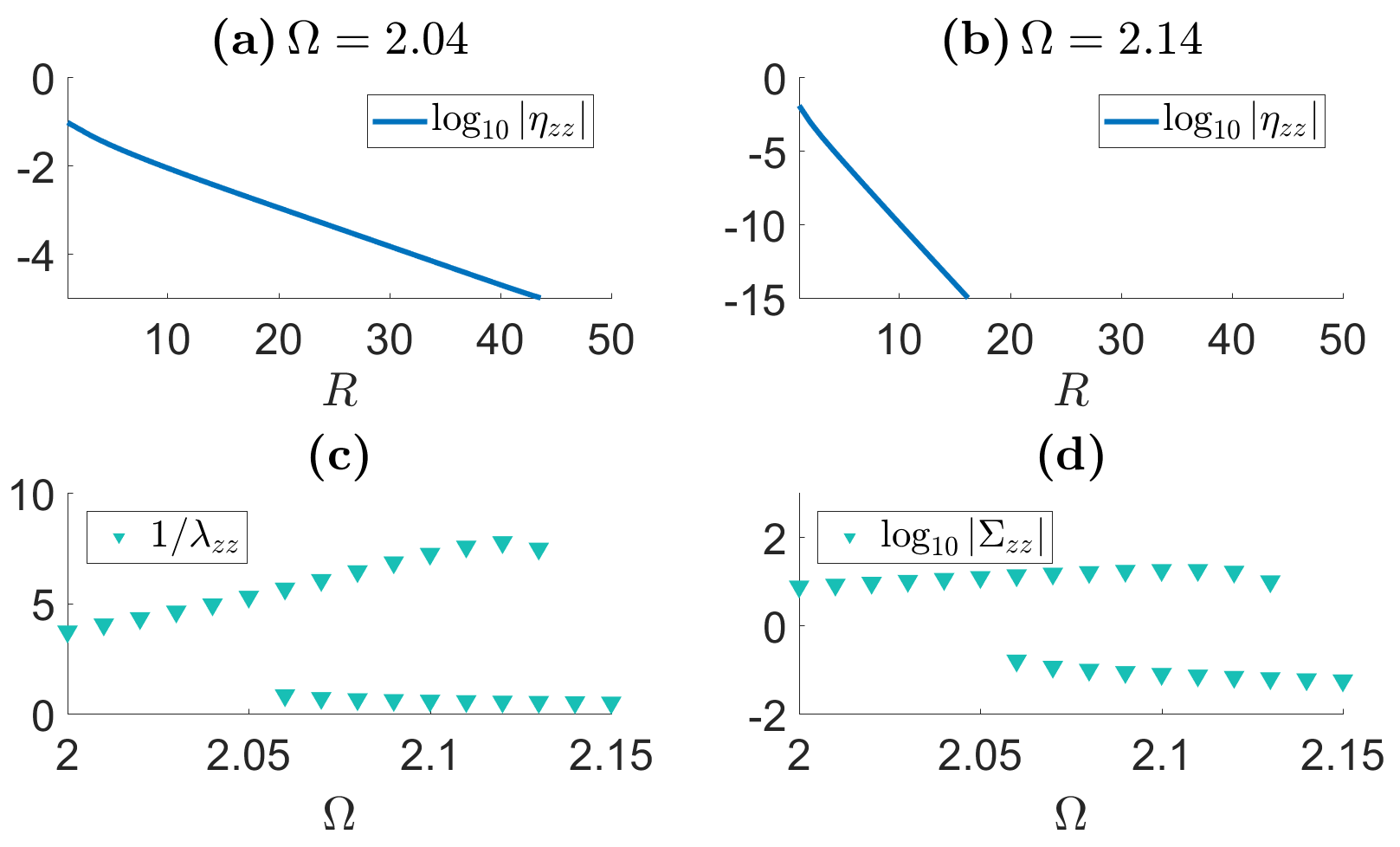
Figure 7: Characteristics of the correlation functions around the bistable region of Fig. 6. (a)-(b) The correlation function $\eta_{zz}(R)$ as a function of the distance for two different $\Omega$ values (outside the bistability region). Note the different scales of the two plots. (c) The correlation length (along one spatial direction) as a function of $\Omega$, showing a difference of up to an order of magnitude in the bistable phases. (d) The total correlation $\Sigma_{zz}=\sum_{R}\eta_{zz}$, showing a difference of up to two orders of magnitude in the bistable phases.

Appendix C 2D-MPO

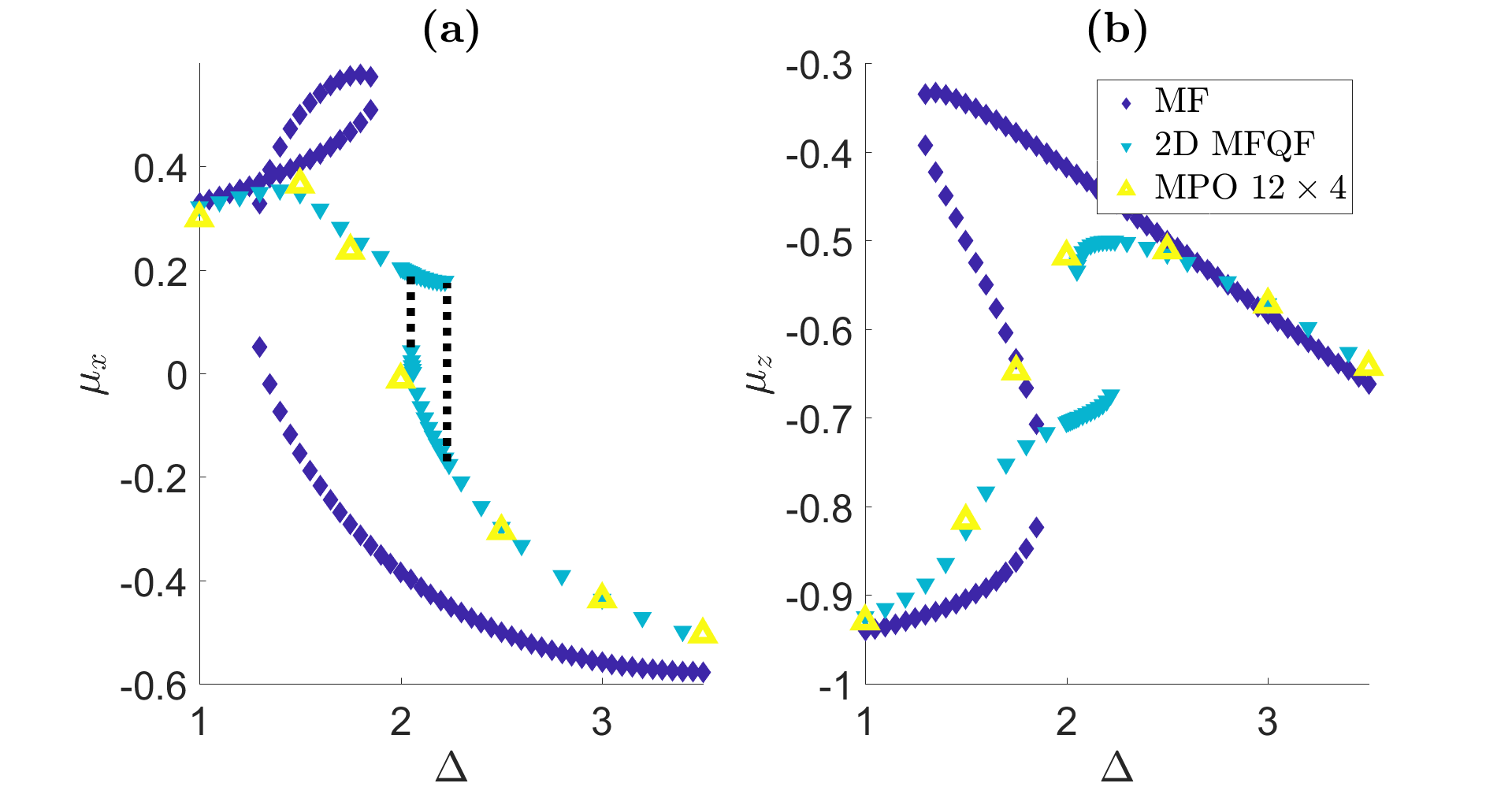
Figure 8: (a) Mean steady-state $x$ magnetization $\mu_{x}^{S}$ and (b) $z$ magnetization $\mu_{z}^{S}$, in the MFQF approximation in 2D, together with the MF limit and 2D-MPO results (for a finite-size, $12\times 4$ cylinder). The parameters are as in Fig. 3 of the main text.

The 2D MPO calculations presented in Fig. 3 of the main text and in Fig. 8, have been carried out on cylinders of length $L_{x}$ from 8 to 16, and fixed $L_{y}=4$. At fixed precision the required bond dimension $\chi$ is expected to be constant with $L_{x}$, but exponentially large in $L_{y}$. The data is obtained with a bond dimension $\chi=400$ (pushed to $\chi=600$ at $\Delta=1.75$). As in the 1D-MPO result, the steady state is obtained by evolving $\rho$ in time from an initial state where all the spins are pointing down. In practice a total time between $15$ and $25$ was used. Since the path of interacting spins associated to the MPO artificially breaks the translation invariance of the lattice in the $y$ direction, it is important to check that the bond dimension is large enough to restore the translation symmetry in the observables. In our case the magnetization was found to be translation invariant up to relative errors of the order of $\mathcal{O}(10^{-4})$.

Appendix D Finite correlation length and mono-modal states

Consider a system where the Liouvilian spectrum has a steady state $\rho_{ss}$, associated to the eigenvalue 0, and an eigenstate $\rho_{E}$ associated to an eigenvalue $\lambda_{E}$ which goes to zero when increasing the system size. We assume that all the other eigenstates are gapped and can be ignored for times $t\gg 1/\Gamma$. As discussed in the main text, there exits two special linear combinations $\rho_{i=1,2}$ of $\rho_{ss}$ and $\rho_{E}$, which are the extreme states [56], and in which local observables have probability distributions with a single peak. On the other hand, nontrivial linear combinations of $\rho_{1}$ and $\rho_{2}$ host bimodal distributions. A natural question is then: what initial conditions lead to $\rho_{1}$ and $\rho_{2}$, and what initial conditions instead lead to some convex combination of the two? We give below a simple heuristic argument suggesting that initial conditions where connected correlation functions have a finite correlation length, should, for a large enough system, lead to one of the two extreme states and not to arbitrary convex combinations of the two. Take an initial state $\rho(t=0)$ where all connected correlation functions are short-ranged. Thanks to the assumption of a gap in the Liouvillian spectrum (above $|\lambda_{E}|$), the state $\rho(t)$ will reach the metastable manifold (spanned by $\rho_{ss}$ and $\rho_{E}$) rather quickly, after a time scale of order $\mathcal{O}(N^{0})$, i.e. a time that is not growing with the system size. Because lattice models with short-range interactions typically have a maximum (Lieb-Robinson) velocity, beyond which the information cannot propagate, it should not be possible for the system to develop true long-range correlations (spanning the whole system) in a finite amount of time. And if correlations remain negligible at distances comparable with the system size, then this implies that the probability distributions of local observable cannot be bi-modal. So, the Lindblad dynamics of a large system initialized from a state with short-range correlations cannot lead to a bimodal state in the time range $1/\Gamma\ll t\ll N^{1/D}$ ($N^{1/D}$ is proportional to the linear size of the system). We thus conclude that in this time window the state that is reached is close to one of the two extreme states, since any other convex combination would be bimodal.

Appendix E Meanfield with Quantum Fluctuations

To derive the equations of the MFQF approach, we define a two-point correlation function (correlator),

$$\vartheta_{ab}(R,R^{\prime},t)\equiv\left\langle\sigma_{R}^{a}\sigma_{R^{\prime}}^{b}\right\rangle,\qquad R\neq R^{\prime},$$ (9)

which is a function of the difference $R-R^{\prime}$ alone, symmetric in $a,b$ (because $\sigma_{R^{\prime}}^{a}$ and $\sigma_{R}^{b}$ commute). Using Eq. (9), the connected two-point correlator is defined as in Eq. (7) of the main text, for $R\neq R^{\prime}$, by

$$\eta_{ab}(R,R^{\prime},t)=\vartheta_{ab}(R,R^{\prime})-\mu_{a}\mu_{b},$$ (10)

The connected three-point correlator is defined for $R\neq R^{\prime}\neq R^{\prime\prime}$ by

$$\zeta_{abc}(R,R^{\prime},R^{\prime\prime},t)\equiv\left\langle\left(\sigma_{R}^{a}-\mu_{a}\right)\left(\sigma_{R^{\prime}}^{b}-\mu_{b}\right)\left(\sigma_{R^{\prime\prime}}^{c}-\mu_{c}\right)\right\rangle,$$ (11)

which is again a function of the differences only.

The approximation of the following treatment is based on assuming that $\zeta$ (and higher order connected correlators) can be neglected in comparison to $\eta$. The e.o.m of $\vartheta_{ab}$, setting $R^{\prime}=0$, is

$$\partial_{t}\vartheta_{ab}(R)=\\ \sum_{d}\Pi_{ad}\vartheta_{db}(R)+\sum_{d}\Pi_{bd}\vartheta_{ad}(R)+f_{ab}(\mu,\vartheta)+g_{ab}(\mu,\vartheta),$$ (12)

where the local Hamiltonian terms are described using the matrix

$$\Pi=\left(\begin{array}[]{ccc}0&-\Delta&0\\ \Delta&0&-2{\Omega}\\ 0&2{\Omega}&0\end{array}\right),$$ (13)

while $f_{ab}(\mu,\vartheta)\propto J$ comes from the kinetic terms, and $g_{ab}(\mu,\vartheta)\propto\Gamma$ comes from the Lindbladian part, and both are given below. By using Eq. (10) we get the e.o.m system for $\eta(R,t)$,

$$\partial_{t}\eta_{ab}(R,t)=\partial_{t}\vartheta_{ab}(R)-\partial_{t}\left[\mu_{a}\mu_{b}\right],$$ (14)

which we solve numerically together with the coupled system for $\vec{\mu}(t)$.

For the Hamiltonian in Eq. (2) of the main text where the kinetic term is

$$-\sum_{\langle R,R^{\prime}\rangle}J\left(\sigma^{+}_{R}\sigma^{-}_{R^{\prime}}+{\rm h.c.}\right)=-\sum_{\langle R,R^{\prime}\rangle}\frac{J}{2}\left(\sigma^{x}_{R}\sigma^{x}_{R^{\prime}}+\sigma^{y}_{R}\sigma^{y}_{R^{\prime}}\right),$$ (15)

we find that $f_{ab}(\mu,\vartheta)$ of Eq. (12) is given by,

$$f_{xx}(R)=2J\left[2\mu_{x}\mu_{y}\mu_{z}-\mu_{x}\vartheta_{yz}(1)-\mu_{y}\vartheta_{xz}(R)\right]\left[\mathcal{Z}-\delta_{\|R\|,1}\right]-2J\sum_{\begin{subarray}{c}R^{\prime}\neq 0\\ \|R^{\prime}-R\|=1\end{subarray}}\mu_{z}\vartheta_{xy}(R^{\prime}),$$ (16)

$$f_{yy}(R)=-2J\left[2\mu_{x}\mu_{y}\mu_{z}-\mu_{y}\vartheta_{xz}(1)-\mu_{x}\vartheta_{yz}(R)\right]\left[\mathcal{Z}-\delta_{\|R\|,1}\right]+2J\sum_{\begin{subarray}{c}R^{\prime}\neq 0\\ \|R^{\prime}-R\|=1\end{subarray}}\mu_{z}\vartheta_{xy}(R^{\prime}),$$ (17)

$$f_{zz}(R)=-2J\left[\mu_{x}\vartheta_{yz}(R)-\mu_{y}\vartheta_{xz}(R)\right]\left[\mathcal{Z}-\delta_{\|R\|,1}\right]-2J\sum_{\begin{subarray}{c}R^{\prime}\neq 0\\ \|R^{\prime}-R\|=1\end{subarray}}\left[\mu_{y}\vartheta_{xz}(R^{\prime})-\mu_{x}\vartheta_{yz}(R^{\prime})\right].$$ (18)

$$f_{xy}(R)=J\left[2\mu_{y}^{2}\mu_{z}-2\mu_{x}^{2}\mu_{z}-\mu_{y}\vartheta_{yz}(1)-\mu_{y}\vartheta_{yz}(R)+\mu_{x}\vartheta_{xz}(1)+\mu_{x}\vartheta_{xz}(R)\right]\left[\mathcal{Z}-\delta_{\|R\|,1}\right]\\ -J\sum_{\begin{subarray}{c}R^{\prime}\neq 0\\ \|R^{\prime}-R\|=1\end{subarray}}\left[\mu_{z}\vartheta_{yy}(R^{\prime})-\mu_{z}\vartheta_{xx}(R^{\prime})\right],$$ (19)

$$f_{xz}(R)=-J\mu_{y}\delta_{\|R\|,1}+J\left[2\mu_{z}^{2}\mu_{y}-\mu_{z}\vartheta_{yz}(1)-\mu_{y}\vartheta_{zz}(R)-\mu_{x}\vartheta_{xy}(R)+\mu_{y}\vartheta_{xx}(R)\right]\left[\mathcal{Z}-\delta_{\|R\|,1}\right]\\ -J\sum_{\begin{subarray}{c}R^{\prime}\neq 0\\ \|R^{\prime}-R\|=1\end{subarray}}\left[\mu_{z}\vartheta_{yz}(R^{\prime})+\mu_{y}\vartheta_{xx}(R^{\prime})-\mu_{x}\vartheta_{xy}(R^{\prime})\right],$$ (20)

$$f_{yz}(R)=J\mu_{x}\delta_{\|R\|,1}+J\left[-2\mu_{z}^{2}\mu_{x}+\mu_{z}\vartheta_{xz}(1)+\mu_{x}\vartheta_{zz}(R)-\mu_{x}\vartheta_{yy}(R)+\mu_{y}\vartheta_{xy}(R)\right]\left[\mathcal{Z}-\delta_{\|R\|,1}\right]\\ +J\sum_{\begin{subarray}{c}R^{\prime}\neq 0\\ \|R^{\prime}-R\|=1\end{subarray}}\left[\mu_{z}\vartheta_{xz}(R^{\prime})-\mu_{y}\vartheta_{xy}(R^{\prime})+\mu_{x}\vartheta_{yy}(R^{\prime})\right].$$ (21)

The components of $g(\mu,\vartheta)$ in Eq. (12) are given by

$$g_{aa}=-\Gamma\vartheta_{aa},\quad g_{xy}=-\Gamma\vartheta_{xy},\quad g_{xz}=-\Gamma\left[2\vartheta_{xz}+\frac{3}{2}\mu_{x}\right],\quad g_{yz}=-\Gamma\left[2\vartheta_{yz}+\frac{3}{2}\mu_{y}\right].$$ (22)

For the Ising model of Eq. (8) where the kinetic term is

$$-\sum_{\langle R,R^{\prime}\rangle}\frac{J_{z}}{2}\sigma^{z}_{R}\sigma^{z}_{R^{\prime}},$$ (23)

we get instead of the above $f_{ab}(\mu,\vartheta)$, the following expressions;

$$f_{xx}(R)=-2J_{z}\left[2\mu_{x}\mu_{y}\mu_{z}-\mu_{x}\vartheta_{yz}(1)-\mu_{z}\vartheta_{xy}(R)\right]\left[\mathcal{Z}-\delta_{\|R\|,1}\right]+2J_{z}\sum_{\begin{subarray}{c}R^{\prime}\neq 0\\ \|R^{\prime}-R\|=1\end{subarray}}\mu_{y}\vartheta_{xz}(R^{\prime}),$$ (24)

$$f_{yy}(R)=2J_{z}\left[2\mu_{x}\mu_{y}\mu_{z}-\mu_{y}\vartheta_{xz}(1)-\mu_{z}\vartheta_{xy}(R)\right]\left[\mathcal{Z}-\delta_{\|R\|,1}\right]-2J_{z}\sum_{\begin{subarray}{c}R^{\prime}\neq 0\\ \|R^{\prime}-R\|=1\end{subarray}}\mu_{x}\vartheta_{yz}(R^{\prime}),$$ (25)

$$f_{zz}(R)=0.$$ (26)

$$f_{xy}(R)=J_{z}\left[2\mu_{x}^{2}\mu_{z}-2\mu_{y}^{2}\mu_{z}-\mu_{x}\vartheta_{xz}(1)-\mu_{z}\vartheta_{xx}(R)+\mu_{y}\vartheta_{yz}(1)+\mu_{z}\vartheta_{yy}(R)\right]\left[\mathcal{Z}-\delta_{\|R\|,1}\right]\\ +J_{z}\sum_{\begin{subarray}{c}R^{\prime}\neq 0\\ \|R^{\prime}-R\|=1\end{subarray}}\left[\mu_{y}\vartheta_{yz}(R^{\prime})-\mu_{x}\vartheta_{xz}(R^{\prime})\right],$$ (27)

$$f_{xz}(R)=J_{z}\mu_{y}\delta_{\|R\|,1}-J_{z}\left[2\mu_{z}^{2}\mu_{y}-\mu_{z}\vartheta_{yz}(1)-\mu_{z}\vartheta_{yz}(R)\right]\left[\mathcal{Z}-\delta_{\|R\|,1}\right]\\ +J_{z}\sum_{\begin{subarray}{c}R^{\prime}\neq 0\\ \|R^{\prime}-R\|=1\end{subarray}}\mu_{y}\vartheta_{zz}(R^{\prime}),$$ (28)

$$f_{yz}(R)=-J_{z}\mu_{x}\delta_{\|R\|,1}+J_{z}\left[2\mu_{z}^{2}\mu_{x}-\mu_{z}\vartheta_{xz}(1)-\mu_{z}\vartheta_{xz}(R)\right]\left[\mathcal{Z}-\delta_{\|R\|,1}\right]\\ -J_{z}\sum_{\begin{subarray}{c}R^{\prime}\neq 0\\ \|R^{\prime}-R\|=1\end{subarray}}\mu_{x}\vartheta_{zz}(R^{\prime}).$$ (29)

References

- Haroche and Raimond (2006) S. Haroche and J. Raimond, Exploring the Quantum: Atoms, Cavities, and Photons, 1st ed. (Oxford University Press, USA, 2006).
- Yamamoto et al. (2000) Y. Yamamoto, F. Tassone, and H. Cao, Semiconductor Cavity Quantum Electrodynamics, 1st ed. (Springer, 2000).
- Schoelkopf and Girvin (2008) R. J. Schoelkopf and S. M. Girvin, “Wiring up quantum systems,” Nature 451, 664 (2008).
- Bardyn et al. (2013) C.-E. Bardyn, M. A. Baranov, C. V. Kraus, E. Rico, A. Imamoğlu, P. Zoller, and S. Diehl, “Topology by dissipation,” New J. Phys. 15, 085001 (2013).
- Oka and Kitamura (2019) T. Oka and S. Kitamura, “Floquet Engineering of Quantum Materials,” Annual Review of Condensed Matter Physics 10, 387 (2019).
- Greentree et al. (2006) A. D. Greentree, C. Tahan, J. H. Cole, and L. C. L. Hollenberg, “Quantum phase transitions of light,” Nature Physics 2, 856 (2006).
- Hartmann et al. (2006) M. J. Hartmann, F. G. S. L. Brandão, and M. B. Plenio, “Strongly interacting polaritons in coupled arrays of cavities,” Nature Physics 2, 849 (2006).
- Chang et al. (2008) D. E. Chang, V. Gritsev, G. Morigi, V. Vuletić, M. D. Lukin, and E. A. Demler, “Crystallization of strongly interacting photons in a nonlinear optical fibre,” Nature Physics 4, 884 (2008).
- Koch et al. (2010) J. Koch, A. A. Houck, K. L. Hur, and S. M. Girvin, “Time-reversal-symmetry breaking in circuit-QED-based photon lattices,” Phys. Rev. A 82, 043811 (2010).
- Petrescu et al. (2012) A. Petrescu, A. A. Houck, and K. Le Hur, “Anomalous Hall effects of light and chiral edge modes on the kagomé lattice,” Phys. Rev. A 86, 053804 (2012).
- Cho et al. (2008) J. Cho, D. G. Angelakis, and S. Bose, “Fractional Quantum Hall State in Coupled Cavities,” Phys. Rev. Lett. 101, 246809 (2008).
- Umucalılar and Carusotto (2011) R. O. Umucalılar and I. Carusotto, “Artificial gauge field for photons in coupled cavity arrays,” Phys. Rev. A 84, 043804 (2011).
- Hafezi et al. (2013) M. Hafezi, M. D. Lukin, and J. M. Taylor, “Non-equilibrium fractional quantum Hall state of light,” New J. Phys. 15, 063001 (2013).
- Rechtsman et al. (2013) M. C. Rechtsman, J. M. Zeuner, Y. Plotnik, Y. Lumer, D. Podolsky, F. Dreisow, S. Nolte, M. Segev, and A. Szameit, “Photonic Floquet topological insulators,” Nature 496, 196 (2013).
- Otterbach et al. (2013) J. Otterbach, M. Moos, D. Muth, and M. Fleischhauer, “Wigner Crystallization of Single Photons in Cold Rydberg Ensembles,” Phys. Rev. Lett. 111, 113001 (2013).
- Carusotto and Ciuti (2013) I. Carusotto and C. Ciuti, “Quantum fluids of light,” Rev. Mod. Phys. 85, 299 (2013).
- Le Hur et al. (2016) K. Le Hur, L. Henriet, A. Petrescu, K. Plekhanov, G. Roux, and M. Schiró, “Many-body quantum electrodynamics networks: Non-equilibrium condensed matter physics with light,” Comptes Rendus Physique 17, 808 (2016).
- Noh and Angelakis (2017) C. Noh and D. G. Angelakis, “Quantum simulations and many-body physics with light,” Rep. Prog. Phys. 80, 016401 (2017).
- Hartmann (2016) M. J. Hartmann, “Quantum simulation with interacting photons,” J. Opt. 18, 104005 (2016).
- Schiró et al. (2016) M. Schiró, C. Joshi, M. Bordyuh, R. Fazio, J. Keeling, and H. Türeci, “Exotic Attractors of the Nonequilibrium Rabi-Hubbard Model,” Phys. Rev. Lett. 116, 143603 (2016).
- Fitzpatrick et al. (2017) M. Fitzpatrick, N. M. Sundaresan, A. C. Y. Li, J. Koch, and A. A. Houck, “Observation of a dissipative phase transition in a one-dimensional circuit qed lattice,” Phys. Rev. X 7, 011016 (2017).
- Fink et al. (2017) J. M. Fink, A. Dombi, A. Vukics, A. Wallraff, and P. Domokos, “Observation of the photon-blockade breakdown phase transition,” Phys. Rev. X 7, 011012 (2017).
- Houck et al. (2012) A. A. Houck, H. E. Türeci, and J. Koch, “On-chip quantum simulation with superconducting circuits,” Nature Physics 8, 292 (2012).
- Schmidt and Koch (2013) S. Schmidt and J. Koch, “Circuit QED lattices: Towards quantum simulation with superconducting circuits,” Ann. Phys. (Berlin) 525, 395 (2013).
- Bloch et al. (2012) I. Bloch, J. Dalibard, and S. Nascimbène, “Quantum simulations with ultracold quantum gases,” Nature Physics 8, 267 (2012).
- Bohnet et al. (2016) J. G. Bohnet, B. C. Sawyer, J. W. Britton, M. L. Wall, A. M. Rey, M. Foss-Feig, and J. J. Bollinger, “Quantum spin dynamics and entanglement generation with hundreds of trapped ions,” Science 352, 1297 (2016).
- Diehl et al. (2010) S. Diehl, A. Tomadin, A. Micheli, R. Fazio, and P. Zoller, “Dynamical phase transitions and instabilities in open atomic many-body systems,” Phys. Rev. Lett. 105, 015702 (2010).
- Sieberer et al. (2013) L. M. Sieberer, S. D. Huber, E. Altman, and S. Diehl, “Dynamical Critical Phenomena in Driven-Dissipative Systems,” Phys. Rev. Lett. 110, 195301 (2013).
- Lee et al. (2013) T. E. Lee, S. Gopalakrishnan, and M. D. Lukin, “Unconventional magnetism via optical pumping of interacting spin systems,” Phys. Rev. Lett. 110, 257204 (2013).
- Jin et al. (2013a) J. Jin, D. Rossini, R. Fazio, M. Leib, and M. J. Hartmann, “Photon solid phases in driven arrays of nonlinearly coupled cavities,” Phys. Rev. Lett. 110, 163605 (2013a).
- Marino and Diehl (2016) J. Marino and S. Diehl, “Driven Markovian Quantum Criticality,” Phys. Rev. Lett. 116, 070407 (2016).
- Scarlatella et al. (2019) O. Scarlatella, R. Fazio, and M. Schiró, “Emergent finite frequency criticality of driven-dissipative correlated lattice bosons,” Phys. Rev. B 99, 064511 (2019).
- Munoz et al. (2019) C. S. Munoz, B. Buča, J. Tindall, A. González-Tudela, D. Jaksch, and D. Porras, “Spontaneous freezing in driven-dissipative quantum systems,” arXiv preprint arXiv:1903.05080 (2019).
- Breuer and Petruccione (2002) H.-P. Breuer and F. Petruccione, The theory of open quantum systems, 1st ed. (Oxford University Press, USA, 2002).
- Lee et al. (2011) T. E. Lee, H. Häffner, and M. C. Cross, “Antiferromagnetic phase transition in a nonequilibrium lattice of Rydberg atoms,” Phys. Rev. A 84, 031402 (2011).
- Qian et al. (2012) J. Qian, G. Dong, L. Zhou, and W. Zhang, “Phase diagram of Rydberg atoms in a nonequilibrium optical lattice,” Phys. Rev. A 85, 065401 (2012).
- Marcuzzi et al. (2014) M. Marcuzzi, E. Levi, S. Diehl, J. P. Garrahan, and I. Lesanovsky, “Universal Nonequilibrium Properties of Dissipative Rydberg Gases,” Phys. Rev. Lett. 113, 210401 (2014).
- Carr et al. (2013) C. Carr, R. Ritter, C. G. Wade, C. S. Adams, and K. J. Weatherill, “Nonequilibrium phase transition in a dilute rydberg ensemble,” Phys. Rev. Lett. 111, 113901 (2013).
- Letscher et al. (2017) F. Letscher, O. Thomas, T. Niederprüm, M. Fleischhauer, and H. Ott, “Bistability versus metastability in driven dissipative rydberg gases,” Phys. Rev. X 7, 021020 (2017).
- Parmee and Cooper (2018) C. D. Parmee and N. R. Cooper, “Phases of driven two-level systems with nonlocal dissipation,” Phys. Rev. A 97, 053616 (2018).
- Jin et al. (2013b) J. Jin, D. Rossini, R. Fazio, M. Leib, and M. J. Hartmann, “Photon solid phases in driven arrays of nonlinearly coupled cavities,” Phys. Rev. Lett. 110, 163605 (2013b).
- Jin et al. (2014) J. Jin, D. Rossini, M. Leib, M. J. Hartmann, and R. Fazio, “Steady-state phase diagram of a driven QED-cavity array with cross-Kerr nonlinearities,” Phys. Rev. A 90, 023827 (2014).
- Foss-Feig et al. (2017) M. Foss-Feig, P. Niroula, J. T. Young, M. Hafezi, A. V. Gorshkov, R. M. Wilson, and M. F. Maghrebi, “Emergent equilibrium in many-body optical bistability,” Phys. Rev. A 95, 043826 (2017).
- Biondi et al. (2017a) M. Biondi, G. Blatter, H. E. Türeci, and S. Schmidt, “Nonequilibrium gas-liquid transition in the driven-dissipative photonic lattice,” Phys. Rev. A 96, 043809 (2017a).
- Chan et al. (2015) C.-K. Chan, T. E. Lee, and S. Gopalakrishnan, “Limit-cycle phase in driven-dissipative spin systems,” Phys. Rev. A 91, 051601 (2015).
- Wilson et al. (2016) R. M. Wilson, K. W. Mahmud, A. Hu, A. V. Gorshkov, M. Hafezi, and M. Foss-Feig, “Collective phases of strongly interacting cavity photons,” Phys. Rev. A 94, 033801 (2016).
- Spohn (1977) H. Spohn, “An algebraic condition for the approach to equilibrium of an open n-level system,” Letters in Mathematical Physics 2, 33 (1977).
- Minganti et al. (2018) F. Minganti, A. Biella, N. Bartolo, and C. Ciuti, “Spectral theory of liouvillians for dissipative phase transitions,” Phys. Rev. A 98, 042118 (2018).
- Weimer (2015) H. Weimer, “Variational Principle for Steady States of Dissipative Quantum Many-Body Systems,” Phys. Rev. Lett. 114, 040402 (2015).
- Biondi et al. (2017b) M. Biondi, S. Lienhard, G. Blatter, H. E. Türeci, and S. Schmidt, “Spatial correlations in driven-dissipative photonic lattices,” New J. Phys. 19, 125016 (2017b).
- Jin et al. (2016) J. Jin, A. Biella, O. Viyuela, L. Mazza, J. Keeling, R. Fazio, and D. Rossini, “Cluster mean-field approach to the steady-state phase diagram of dissipative spin systems,” Phys. Rev. X 6, 031011 (2016).
- Daley (2014) A. J. Daley, “Quantum trajectories and open many-body quantum systems,” Adv. Phys. 63, 77 (2014).
- Prosen and Žnidarič (2009) T. Prosen and M. Žnidarič, “Matrix product simulations of non-equilibrium steady states of quantum spin chains,” J. Stat. Mech. 2009, P02035 (2009).
- Mendoza-Arenas et al. (2016) J. J. Mendoza-Arenas, S. R. Clark, S. Felicetti, G. Romero, E. Solano, D. G. Angelakis, and D. Jaksch, “Beyond mean-field bistability in driven-dissipative lattices: Bunching-antibunching transition and quantum simulation,” Phys. Rev. A 93, 023821 (2016).
- Vicentini et al. (2018) F. Vicentini, F. Minganti, R. Rota, G. Orso, and C. Ciuti, “Critical slowing down in driven-dissipative Bose-Hubbard lattices,” Phys. Rev. A 97, 013853 (2018).
- Jin et al. (2018) J. Jin, A. Biella, O. Viyuela, C. Ciuti, R. Fazio, and D. Rossini, “Phase diagram of the dissipative quantum ising model on a square lattice,” Phys. Rev. B 98, 241108 (2018).
- Kshetrimayum et al. (2017) A. Kshetrimayum, H. Weimer, and R. Orús, “A simple tensor network algorithm for two-dimensional steady states,” Nature Comm. 8, 1291 (2017).
- Cai and Barthel (2013) Z. Cai and T. Barthel, “Algebraic versus Exponential Decoherence in Dissipative Many-Particle Systems,” Phys. Rev. Lett. 111, 150403 (2013).
- Macieszczak et al. (2016) K. Macieszczak, M. Guţă, I. Lesanovsky, and J. P. Garrahan, “Towards a Theory of Metastability in Open Quantum Dynamics,” Phys. Rev. Lett. 116, 240404 (2016).
- (60) “See supplemental material.” .
- (61) H. Landa, M. Schiró, and G. Misguich, “In preparation,” .
- Mascarenhas et al. (2015) E. Mascarenhas, H. Flayac, and V. Savona, “Matrix-product-operator approach to the nonequilibrium steady state of driven-dissipative quantum arrays,” Phys. Rev. A 92, 022116 (2015).
- Schollwöck (2011) U. Schollwöck, “The density-matrix renormalization group in the age of matrix product states,” Annals of Physics 326, 96 (2011), january 2011 Special Issue.
- Zaletel et al. (2015) M. P. Zaletel, R. S. K. Mong, C. Karrasch, J. E. Moore, and F. Pollmann, “Time-evolving a matrix product state with long-ranged interactions,” Phys. Rev. B 91, 165112 (2015).
- Benenti et al. (2009) G. Benenti, G. Casati, T. Prosen, D. Rossini, and M. Žnidarič, “Charge and spin transport in strongly correlated one-dimensional quantum systems driven far from equilibrium,” Phys. Rev. B 80, 035110 (2009).
- ite (n 21) ITensor Library, http://itensor.org (version 2.1).
- Bidzhiev and Misguich (2017) K. Bidzhiev and G. Misguich, “Out-of-equilibrium dynamics in a quantum impurity model: Numerics for particle transport and entanglement entropy,” Phys. Rev. B 96, 195117 (2017).
- Stoudenmire and White (2012) E. Stoudenmire and S. R. White, “Studying Two-Dimensional Systems with the Density Matrix Renormalization Group,” Annu. Rev. Condens. Matter Phys. 3, 111 (2012).
- Rose et al. (2016) D. C. Rose, K. Macieszczak, I. Lesanovsky, and J. P. Garrahan, “Metastability in an open quantum Ising model,” Phys. Rev. E 94, 052132 (2016).
- Casteels et al. (2017) W. Casteels, R. Fazio, and C. Ciuti, “Critical dynamical properties of a first-order dissipative phase transition,” Phys. Rev. A 95, 012128 (2017).
- Porras and Cirac (2004) D. Porras and J. I. Cirac, “Effective quantum spin systems with trapped ions,” Phys. Rev. Lett. 92, 207901 (2004).
- Friedenauer et al. (2008) A. Friedenauer, H. Schmitz, J. T. Glueckert, D. Porras, and T. Schaetz, “Simulating a quantum magnet with trapped ions,” Nature Physics 4, 757 (2008).
- Schneider et al. (2012) C. Schneider, D. Porras, and T. Schaetz, “Experimental quantum simulations of many-body physics with trapped ions,” Reports on Progress in Physics 75, 024401 (2012).
- Islam et al. (2013) R. Islam, C. Senko, W. C. Campbell, S. Korenblit, J. Smith, A. Lee, E. E. Edwards, C.-C. J. Wang, J. K. Freericks, and C. Monroe, “Emergence and Frustration of Magnetism with Variable-Range Interactions in a Quantum Simulator,” Science 340, 583 (2013).
- Smith et al. (2016) J. Smith, A. Lee, P. Richerme, B. Neyenhuis, P. W. Hess, P. Hauke, M. Heyl, D. A. Huse, and C. Monroe, “Many-body localization in a quantum simulator with programmable random disorder,” Nature Physics 12, 907 (2016).