Minimax Rates of Estimating Approximate Differential Privacy

Abstract

Differential privacy has become a widely accepted notion of privacy, leading to the introduction and deployment of numerous privatization mechanisms. However, ensuring the privacy guarantee is an error-prone process, both in designing mechanisms and in implementing those mechanisms. Both types of errors will be greatly reduced, if we have a data-driven approach to verify privacy guarantees, from a black-box access to a mechanism. We pose it as a property estimation problem, and study the fundamental trade-offs involved in the accuracy in estimated privacy guarantees and the number of samples required. We introduce a novel estimator that uses polynomial approximation of a carefully chosen degree to optimally trade-off bias and variance. With $n$ samples, we show that this estimator achieves performance of a straightforward plug-in estimator with $n\ln n$ samples, a phenomenon referred to as effective sample size amplification. The minimax optimality of the proposed estimator is proved by comparing it to a matching fundamental lower bound.

1 Introduction

Differential privacy is gaining popularity as an agreed upon measure of privacy leakage, widely used by the government to publish Census statistics [Abo18], Google to aggregate user’s choices in web-browser features [EPK14, FPE16], Apple to aggregate mobile user data [Tea17], and smart meters in telemetry [DKY17]. As increasing number of privatization mechanisms are introduced and deployed in the wild, it is critical to have countermeasures to check the fidelity of those mechanisms. Such techniques will allow us to hold accountable the deployment of privatization mechanisms if the claimed privacy guarantees are not met, and find and fix bugs in implementations of those mechanisms.

A user-friendly tool for checking privacy guarantees is necessary for several reasons. Writing a program for a privatization mechanism is error-prone, as it involves complex probabilistic computations. Even with customized languages for differential privacy, checking the end-to-end privacy guarantee of an implementation remains challenging [BKOZB12, WDW⁺19]. Furthermore, even when the implementation is error-free, there have been several cases where the mechanism designers have made errors in calculating the privacy guarantees, and falsely reported higher level of privacy [LSL17, CM15]. This is evidence of an alarming issue that analytically checking the proof of a privacy guarantee is a challenging process even for an expert. An automated and data-driven algorithm for checking privacy guarantees will significantly reduce such errors in the implementation and the design. On other cases, we are given very limited information about how the mechanism works, like Apple’s white paper [Tea17]. The users are left to trust the claimed privacy guarantees.

To address these issues, we propose a data-driven approach to estimate how much privacy is guaranteed, from a black-box access to a purportedly private mechanism. Our approach is based on an optimal polynomial approximation that gracefully trades off bias and variance. We study the fundamental limit of how many samples are necessary to achieve a desired level of accuracy in the estimation, and show that the proposed approach achieves this fundamental bound.

Problem formulation. Differential privacy (DP) introduced in [Dwo11] is a formal mathematical notion of privacy that is widespread, due to several key advantages. It gives one of the strongest guarantees, allows for precise mathematical analyses, and is intuitive to explain even to non-technical end-users. When accessing a database through a query, we say the query output is private if the output did not reveal whether a particular person’s entry is in the database or not. Formally, we say two databases are neighboring if they only differ in one entry (one row in a table, for example). Let $P_{{\cal Q},{\cal D}}$ denote the distribution of the randomized output to a query ${\cal Q}$ on a database ${\cal D}$. We consider discrete valued mechanisms taking one of $S$ values, i.e. the response to a query is in $[S]=\{1,\ldots,S\}$ for some integer $S$. We say a mechanism guarantees $(\varepsilon,\delta)$-DP, [Dwo11], if the following holds

$$P_{{\cal Q},{\cal D}}(E)\;\leq\;e^{\varepsilon}P_{{\cal Q},{\cal D}^{\prime}}(E)+\delta\;,$$ (1)

for some $\varepsilon\geq 0$, $\delta\in[0,1]$, and all subset $E\subseteq[S]$ and for all neighboring databases ${\cal D}$ and ${\cal D}^{\prime}$. When $\delta=0$, $(\varepsilon,0)$-DP is referred to as (pure) differential privacy, and the general case of $\delta\geq 0$ is referred to as approximate differential privacy. For pure DP, the above condition can be relaxed as

$$P_{{\cal Q},{\cal D}}(x)\;\leq\;e^{\varepsilon}P_{{\cal Q},{\cal D}^{\prime}}(x)\;,$$ (2)

for all output symbol $x\in[S]$, and for all neighboring databases ${\cal D}$ and ${\cal D}^{\prime}$. This condition can now be checked, one symbol $x$ at a time from $[S]$, without having to enumerate all subsets $E\subseteq[S]$. This naturally leads to the following algorithm.

For a query ${\cal Q}$ and two neighboring databases ${\cal D}$ and ${\cal D}^{\prime}$ of interest, we need to verify the condition in Eq. (2). As we only have a black-box access to the mechanism, we collect $n$ responses from the mechanism on the two databases. We check the condition on the empirical distribution of those collected samples, for each $x\in[S]$. If it is violated for any $x$, we assert the mechanism to be not $(\varepsilon,0)$-DP and present $x$ as an evidence. Focusing only on pure DP, [DWW⁺18] proposed an approach similar to this, where they also give guidelines for choosing the databases ${\cal D}$ and ${\cal D}^{\prime}$ to test. However, their approach is only evaluated empirically, no statistical analysis is provided, and a more general case of approximate DP is left as an open question, as the condition in Eq. (1) cannot be decoupled like Eq. (2) when $\delta>0$.

We propose an alternative approach from first principles to check the general approximate DP guarantees, and prove its minimax optimality. Given two probability measures $P=[p_{1},\ldots,p_{S}]$ and $Q=[q_{1},\ldots,q_{S}]$ over $[S]=\{1,\ldots,S\}$, we define the following approximate DP divergence with respect to $\varepsilon$ as

$$d_{\varepsilon}(P\|Q)\;\;\triangleq\;\;\sum_{i=1}^{S}[p_{i}-e^{\varepsilon}q_{i}]^{+}\;\;=\;\;\mathbb{E}_{x\sim P}\Big{[}\,\Big{[}1-e^{\varepsilon}\frac{q_{x}}{p_{x}}\Big{]}^{+}\,\Big{]}\;.$$ (3)

where $[x]^{+}=\max\{x,0\}$. The last representation indicates that this metric falls under a broader class of metrics known as $f$-divergences, with a special choice of $f(x)=[1-e^{\varepsilon}x]^{+}$. From the definition of DP, it follows that a mechanism is $(\varepsilon,\delta)$-DP if and only if $d_{\varepsilon}(P_{{\cal Q},{\cal D}}\|P_{{\cal Q},{\cal D}^{\prime}})\leq\delta$ for all neighboring databases ${\cal D}$ and ${\cal D}^{\prime}$. We propose estimating this divergence $d_{\varepsilon}(P_{{\cal Q},{\cal D}}\|P_{{\cal Q},{\cal D}^{\prime}})$ from samples, and comparing it to the target $\delta$. This only requires number of operations scaling as $S\ln n$ where $n$ is the sample size.

In this paper, we suppose there is a specific query ${\cal Q}$ of interest, and two neighboring databases ${\cal D}$ and ${\cal D}^{\prime}$ have been already selected either by a statistician who has some side information on the structure of the mechanism or by some algorithm, such as those from [DWW⁺18]. Without exploiting the structure (such as symmetry, exchangeability, or invariance to the entries of the database conditioned on the true output of the query), one cannot avoid having to check all possible combinations of neighboring databases. As a remedy, [GM18] proposes checking randomly selected databases. This in turn ensures a relaxed notion of privacy known as random differential privacy. Similarly, [DJRT13] proposed checking the typical databases, assuming there we have access to a prior distribution over the databases. Our framework can be seamlessly incorporated with such higher-level routines to select databases.

Contributions. We study the problem of estimating the approximate differential privacy guaranteed by a mechanism, from a black-box access where we can sample from the mechanism output given a query ${\cal Q}$, a database ${\cal D}$, and a target $(\varepsilon,\delta)$. We first show that a straightforward plug-in estimator of $d_{\varepsilon}(P\|Q)$ achieves mean squared error scaling as $(e^{\varepsilon}S)/n$, where $S$ is the size of the alphabet and $n$ is the number of samples used (Section 2.1.1).

In the regime where we fix $S$ and increase the sample size, this achieves the parametric rate of $1/n$, and cannot be improved upon. However, in many cases of practical interest where $S$ is comparable to $n$, we show that this can be improve upon with a more sophisticated estimator. To this end, we introduce a novel estimator of $d_{\varepsilon}(P\|Q)$. The main idea is to identify the regimes of non-smoothness in $[p_{i}-e^{\varepsilon}q_{i}]^{+}$ where the plug-in estimator has a large bias. We replace it by the uniformly best polynomial approximation of the non-smooth regime of the function, and estimate those polynomial from samples. By selecting appropriate degree of the polynomial, we can optimally trade off the bias and variance. We provide an upper bound on the error scaling as $(e^{\varepsilon}S)/(n\ln n)$, when $S$ and $n$ are comparable. We prove that this is the best one can hope for, by providing a minimax lower bound that matches.

We first show this for the case when we know $P$ and sample from $Q$ in Section 2.1, to lay out the main technical insights while maintaining simple exposition. Then, we consider the practical scenario where both $P$ and $Q$ are accessed via samples, and provide an minimax optimal estimator in Section 2.2. This phenomenon is referred to as effective sample size amplification; one can achieve with $n$ samples a desired error rate, that would require $n\ln n$ samples for a plug-in estimator. We present numerical experiments supporting our theoretical predictions in Section 3, and use our estimator to identify those real-world and artificial mechanisms that have incorrectly reported the privacy guarantees.

Related work. Formally guaranteeing differential privacy is a challenging and error-prone task. Principled approaches have been introduced to derive the end-to-end privacy loss of a software program that uses multiple differentially private accesses to the data, including SQL-based languages [McS09], higher-order functional languages [RP10], and imperative languages [CGLN11]. A unifying recipe of these approaches is to combine standard mechanisms like Laplacian, exponential, and Gaussian mechanisms [Dwo11, MT07, GKOV15], and calculate the end-to-end privacy loss using the composition theorem [KOV17]. To extend these approaches to a more general notion of approximate differential privacy and allow non-standard components, principled approaches have been proposed in [BKOZB12, WDW⁺19]. The main idea is to perform fine-grained reasoning about the complex probabilistic computations involved. These existing approaches have been preemptive measures aimed at automated verification of privacy of the source code. Instead, we seek a post-hoc measure of estimating the privacy guarantee, given a black-box access to a privatization mechanism and not the source code.

Several published mechanisms have mistakes in the privacy guarantees. These are variations of a popular mechanism known as Sparse Vector Technique (SVT). The original SVT first generates a random threshold. To answer a sequence of queries, it adds a random noise to each query output, and respond whether this is higher than the threshold (true) or not (false). This process continues until either all queries are answered, each with a privatized Boolean response or if the number of trues meets a pre-defined bound. Several variations violate claimed DP guarantees. [SCM14] proposes variant of SVT with no noise adding and no bound on the number of trues, which does not satisfy DP for any values of $\varepsilon$. [CXZX15] makes a similar false claim, proposing a version of SVT with no bound on the number of trues. [LC14] adds a smaller noise independent of the bound on the trues. [Rot11] outputs the actual noisy vector instead of the Boolean vector.

A formal investigation into verifying DP guarantees of a given mechanism was addressed in [DJRT13]. DP condition is translated into a certain Lipschitz condition on $P_{{\cal Q},{\cal D}}$ over the databases ${\cal D}$, and a Lipschitz tester is proposed to check the conditions. However, this approach is not data driven, as it requires the knowledge of the distribution $P_{{\cal Q},{\cal D}}$ and no sampling of the mechanism outputs is involved. [GM18] analyzes tradeoffs involved in testing DP guarantees. It is shown that one cannot get accurate testing without sacrificing the privacy of the databases used in the testing. Hence, when testing DP guarantees, one should not use databases that contain sensitive data. We compare some of the techniques involved in Section 2.1.1.

Our techniques are inspired by a long line of research in property estimation of a distribution from samples. In particular, there has been significant recent advances for high-dimensional estimation problems, starting from entropy estimation for discrete random variables in [VV13, JVHW15, WY16]. The general recipe is to identify the regime where the property to be estimated is not smooth, and use functional approximation to estimate a smoothed version of the property. This has been widely successful in support recovery [WY19], density estimation with $\ell_{1}$ loss [HJW15], and estimating Renyi entropy [AOST17]. more recently, this technique has been applied to estimate certain divergences between two unknown distributions, for Kullback-Leibler divergence [HJW16], total variation distance [JHW18], and identity testing [DKW18]. With carefully designed estimators, these approximation-based approaches can achieve improvement over typical parametric rate of $1/n$ error rate, sometimes referred to as effective sample size amplification.

Notations. We let the alphabet of a discrete distribution be $[S]=\{1,\ldots,S\}$ for some positive integer $S$ denoting the size of the alphabet. We let ${\cal M}_{S}$ denote the set of probability distributions over $[S]$. We use $f(n)\gtrsim g(n)$ to denote that $\sup_{n}f(n)/g(n)\geq C$ for some constant $C$, and $f(n)\lesssim g(n)$ is analogously defined. $f(n)\asymp g(n)$ denotes that $f(n)\gtrsim g(n)$ and $f(n)\lesssim g(n)$.

2 Estimating differential privacy guarantees from samples

We want to estimate $d_{\varepsilon}(P\|Q)$ from a blackbox access to the mechanism outputs accessing two databases, i.e. $P=P_{{\cal Q},{\cal D}}$ and $Q=P_{{\cal Q},{\cal D}^{\prime}}$. We first consider a simpler case, where $P=[p_{1},\ldots,p_{S}]$ is known and we observe samples from an unknown distribution $Q=[q_{1},\ldots,q_{S}]$ in Section 2.1. We cover this simpler case first to demonstrate the main ideas on the algorithm design and analysis technique while maintaining the exposition simple. This paves the way for our main algorithmic and theoretical results in Section 2.2, where we only have access to samples from both $P$ and $Q$.

2.1 Estimating $d_{\varepsilon}(P\|Q)$ with known P

For a given budget $n$, representing an upper bound on the expected number of samples we can collect, we propose sampling a random number $N$ of samples from Poisson distribution with mean $n$, i.e. $N\sim{\rm Poi}\,(n)$. Then, each sample $X_{j}\in[S]$ is drawn from $Q$ for $j\in\{1,\ldots,N\}$, and we let $Q_{n}=[{\hat{q}}_{1},\ldots,{\hat{q}}_{S}]$ denote the resulting histogram divided by $n$, such that ${\hat{q}}_{i}\triangleq|\{j\in[N]:X_{i}=j\}|/n$.

Note that $Q_{n}$ is not the standard empirical distribution, as $\sum_{i}{\hat{q}}_{i}\neq 1$ with high probability. However, in this paper we refer to $Q_{n}$ as empirical distribution of the samples. The empirical distribution would have been divided by $N$ instead of $n$. Instead, $Q_{n}$ is the maximum likelihood estimate of the true distribution $Q$. This Poisson sampling, together with the MLE construction of $Q_{n}$, ensures independence among $\{{\hat{q}}_{i}\}_{i=1}^{S}$, making the analysis simpler. We first analyze the sample complexity of a simple plug-in estimator $d_{\varepsilon}(P\|Q_{n})$ in Section 2.1.1. This is well-defined regardless of whether $Q_{n}$ sums to one or not. We next show that we can significantly improve the sample complexity by using a novel estimator, Algorithm 1, in Section 2.1.2. We show minimax optimality of the proposed estimator by proving a matching lower bound in Section 2.1.3.

2.1.1 Performance of the plug-in estimator

The following result shows that it is necessary and sufficient to have $n\approx e^{\varepsilon}\,S$ samples to achieve an arbitrary desired error rate, if we use this plug-in estimator $d_{\varepsilon}(P\|Q_{n})$, under the worst-case $P$ and $Q$. Some assumption on $(P,Q)$ is inevitable as it is trivial to achieve zero error for any sample size, for example if $P$ and $Q$ have disjoint supports. Both $d_{\varepsilon}(P\|Q)$ and $d_{\varepsilon}(P\|Q_{n})$ are 1 with probability one. We provide a proof in Section 4.2. The bound in Eq. (6) also holds for $d_{\varepsilon}(P_{n}\|Q)$. The proof technique is analogous, and we omit the proof here.

Theorem 1.

For any $\varepsilon\geq 0$, support size $S\in\mathbb{Z}^{+}$, and distribution $P\in{\cal M}_{S}$, the plug-in estimator satisfies

$$\sup_{Q\in{\cal M}_{S}}\mathbb{E}_{Q}\big{[}\,|d_{\varepsilon}(P\|Q_{n})-d_{\varepsilon}(P\|Q)|^{2}\,\big{]}\;\;\lesssim\;\;\Big{(}\,\sum_{i=1}^{S}\,p_{i}\wedge\sqrt{\frac{e^{\varepsilon}p_{i}}{n}}\,\Big{)}^{2}+\frac{e^{\varepsilon}}{n}\;,$$ (4)

with expected number of samples $n$. If $S\geq 2$, we can also lower bound the worst case mean squared error as

$$\sup_{Q\in{\cal M}_{S}}\mathbb{E}_{Q}\big{[}\,|d_{\varepsilon}(P\|Q_{n})-d_{\varepsilon}(P\|Q)|^{2}\,\big{]}\;\;\gtrsim\;\;\Big{(}\,\sum_{i=1}^{S}\,p_{i}\wedge\sqrt{\frac{e^{\varepsilon}p_{i}}{n}}\,\Big{)}^{2}\;.$$ (5)

When $n\geq e^{\varepsilon}S$, it follows that right-hand side of the lower bound is at least $e^{\varepsilon}S/n$, and the matching upper and lower bounds can be simplified as follows, for the worst case $P$ and $Q$.

Corollary 2.

If $n\geq e^{\varepsilon}S$ and $S\geq 2$, we have

$$\sup_{P,Q\in{\cal M}_{S}}\mathbb{E}_{Q}\big{[}\,|d_{\varepsilon}(P\|Q_{n})-d_{\varepsilon}(P\|Q)|^{2}\,\big{]}\;\;\asymp\;\;\frac{e^{\varepsilon}S\,}{n}\;.$$ (6)

A similar analysis was done in [GM18], which gives an upper bound scaling as $e^{2\varepsilon}S/n$. We tighten the analysis by a factor of $e^{\varepsilon}$, and provide a matching lower bound.

2.1.2 Achieving optimal sample complexity with a polynomial approximation

We construct a minimax optimal estimator using techniques first introduced in [WY16, JVHW15] and adopted in several property estimation problems including [HJW15, HJW16, AOST17, JHW18, DKW18, WY19].

0:  target privacy $\varepsilon\in{\mathbb{R}}^{+}$, query ${\cal Q}$, neighboring databases $({\cal D},{\cal D}^{\prime})$, pmf of $P_{{\cal Q},{\cal D}}$ samples from $P_{{\cal Q},{\cal D}^{\prime}}$, degree $K\in{\mathbb{Z}}^{+}$, constants $c_{1},c_{2}\in{\mathbb{R}}^{+}$, expected sample size $2n$

0:  estimate ${\widehat{d}}_{\varepsilon,K,c_{1},c_{2}}(P\|Q_{n})$ of $d_{\varepsilon}(P_{{\cal Q},{\cal D}}\|P_{{\cal Q},{\cal D}^{\prime}})$

  $P\leftarrow P_{{\cal Q},{\cal D}}$

  Draw two independent sample sizes: $N_{1}\leftarrow{\rm Poi}\,(n)$ and $N_{2}\leftarrow{\rm Poi}\,(n)$

  Sample from $P_{{\cal Q},{\cal D}^{\prime}}$: $\{X_{i,1}\}_{i=1}^{N_{1}}\in[S]^{N_{1}}$ and $\{X_{i,2}\}_{i=1}^{N_{2}}\in[S]^{N_{2}}$

  ${\hat{q}}_{i,j}\leftarrow\frac{|\{\ell\in[N_{j}]:X_{\ell,j}=i\}|}{n}$ for all $i\in[S]$ and $j\in\{1,2\}$

  $Q_{n,1}\leftarrow[{\hat{q}}_{1,1},\ldots,{\hat{q}}_{S,1}]$ and $Q_{n,2}\leftarrow[{\hat{q}}_{1,2},\ldots,{\hat{q}}_{S,2}]$

  for $i=1$ to $S$ do

                       $\delta_{i}\leftarrow\left\{\begin{array}[]{rl}0&,\;\text{ if }{\hat{q}}_{i,1}>U(p_{i};c_{1},c_{2})\\ {\tilde{D}}_{K}({\hat{q}}_{i,2};p_{i})&,\;\text{ if }{\hat{q}}_{i,1}\in U(p_{i};c_{1},c_{2})\\ {[p_{i}-e^{\varepsilon}{\hat{q}}_{i,2}]^{+}}&,\;\text{ if }{\hat{q}}_{i,1}<U(p_{i};c_{1},c_{2})\end{array}\right.$

  end for

  ${\widehat{d}}_{\varepsilon,K,c_{1},c_{2}}(P\|Q_{n})\leftarrow 0\vee(1\wedge\sum_{i=1}^{S}\delta_{i}$)

Algorithm 1 Differential Privacy (DP) estimator with known $P$

To simplify the analysis, we split the samples randomly into two partitions, each having an independent and identical distribution of ${\rm Poi}\,(n)$ samples from the multinomial distribution $Q$. We let $Q_{n,1}=[{\hat{q}}_{1,1},\ldots,{\hat{q}}_{S,1}]$ denote the count of the first set of $N_{1}\sim{\rm Poi}\,(n)$ samples (normalized by $n$), and $Q_{n,2}=[{\hat{q}}_{1,1},\ldots,{\hat{q}}_{S,1}]$ the second set of $N_{2}\sim{\rm Poi}\,(n)$ samples. See Algorithm 1 for a formal definition. Note that for the analysis we are collecting $2n$ samples in total on average. In all the experiments, however, we apply our estimator without partitioning the samples. A major challenge in achieving the minimax optimality is in handling the non-smoothness of the function $f({\hat{q}}_{i};p_{i})\triangleq[p_{i}-e^{\varepsilon}{\hat{q}}_{i}]^{+}$ at $p_{i}\simeq e^{\varepsilon}{\hat{q}}_{i}$. We use one set of samples to identify whether an outcome $i\in[S]$ is in the smooth regime (${\hat{q}}_{i,1}\notin U(p;c_{1},c_{2})$) or not (${\hat{q}}_{i,1}\in U(p;c_{1},c_{2})$), with an appropriately defined set function:

$$U(p;c_{1},c_{2})\;\;\triangleq\;\;\left\{\begin{array}[]{rl}{[0,\frac{(c_{1}+c_{2})\ln n}{n}]}&,\;\text{ if }p\leq\frac{c_{1}e^{\varepsilon}\ln n}{n}\;,\\ {\Big{[}e^{-\varepsilon}p-\sqrt{\frac{c_{2}e^{-\varepsilon}p\ln n}{n}},e^{-\varepsilon}p+\sqrt{\frac{c_{2}e^{-\varepsilon}p\ln n}{n}}\Big{]}}&,\;\text{ otherwise},\\ \end{array}\right.$$ (9)

for $c_{1}\geq c_{2}>0$ and $p\in[0,1]$. The scaling of the interval is chosen carefully such that $(a)$ it is large enough for the probability of making a mistake on the which regime $(p_{i},q_{i})$ falls into to vanishes (Lemma 14); and $(b)$ it is small enough for the variance of the polynomial approximation in the non-smooth regime to match that of the other regimes (Lemma 15). In the smooth regime, we use the plug-in estimator. In the non-smooth regime, we can improve the estimation error by using the best polynomial approximation of $f(x;p_{i})=[p_{i}-e^{\varepsilon}\,x]^{+}$, which has a smaller bias:

$$D_{K}(x;p)\;\;\triangleq\;\;\operatorname*{arg\,min}_{P\in{\rm poly_{K}}}\max_{\tilde{x}\in U(p;c_{1},c_{1})}\big{|}\,[p-e^{\varepsilon}\tilde{x}]^{+}-P(\tilde{x})\,\big{|}\;,$$ (10)

where ${\rm poly_{K}}$ is the set of polynomial functions of degree at most $K$, and we approximate $f(x;p)$ in an interval $U(p;c_{1},c_{1})\supset U(p;c_{1},c_{2})$ for any $c_{1}>c_{2}$. Having this slack of $c_{1}>c_{2}$ in the approximation allows us to guarantee the approximation quality, even if the actual $q_{i}$ is not exactly in the non-smooth regime $U(p;c_{1},c_{2})$. Once we have the polynomial approximation, we estimate this polynomial function $D_{K}(q_{i};p_{i})$ from samples, using the uniformly minimum variance unbiased estimator (MVUE).

There are several advantages that makes this two-step process attractive. As we use an unbiased estimate of the polynomial, the bias is exactly the polynomial approximation error of $D_{K}(x;p_{i})$, which scales as $(1/K)\sqrt{(p_{i}\ln n)/n}$. Larger degree $K$ reduces the approximation error, and larger $n$ reduces the support of the domain we apply the approximation to in $U(p;c_{1},c_{1})$ (Lemma 15). The variance is due to the sample estimation of the polynomial $D_{K}(x;p_{i})$, which scales as $(B^{K}p_{i}\ln n)/n$ for some universal constant $B$ (Lemma 15). Larger degree $K$ increases the variance. We prescribe choosing $K=c_{3}\ln n$ for appropriate constant $c_{3}$ to optimize the bias-variance tradeoff in Algorithm 1. The resulting two-step polynomial estimator, has two characterizations, depending on where $p_{i}$ is. Let $\Delta=(c_{1}\ln n)/n$.

Case 1: $p_{i}\leq e^{\varepsilon}\Delta$ and ${\hat{q}}_{i}\in U(p_{i};c_{1},c_{1})=[0,2\Delta]$. We consider the function $g(y)=[p_{i}-e^{\varepsilon}2\Delta y]^{+}$ by substituting $2\Delta y=x$ into $f(p_{i},x)=[p_{i}-e^{\varepsilon}x]^{+}$. Let $H_{K}(y)$ be the best polynomial approximation of $g(y)\in C[0,1]$ with order $K$, i.e. $H_{K}(y)=\operatorname*{arg\,min}_{P\in{\rm poly_{K}}}\max_{y^{\prime}\in[0,1]}\big{|}\,g(y^{\prime})-P(y^{\prime})\,\big{|}$ and denote it as $H_{K}(y)=\sum_{j=0}^{K}a_{j}y^{j}$. Then $D_{K}(x;p_{i})=H_{K}({x}/({2\Delta}))=\sum_{j=0}^{K}a_{j}(2\Delta)^{-j}x^{j}$. Once we have the polynomial approximation, we estimate with the uniformly minimum variance unbiased estimator (MVUE) to estimate $D_{K}({\hat{q}}_{i};p_{i})$.

$${\tilde{D}}_{K}({\hat{q}}_{i};p_{i})\;\;=\;\;\sum_{j=0}^{K}a_{j}(2\Delta)^{-j}\prod_{k=0}^{j-1}({\hat{q}}_{i}-\frac{k}{n})\;.$$ (11)

Computing the $a_{j}$’s can be challenging, and we discuss this for the general case when $P$ is not known in Section 2.2.

Case 2: $p_{i}>e^{\varepsilon}\Delta$ and ${\hat{q}}_{i}\in[e^{-\varepsilon}p_{i}-\sqrt{e^{-\varepsilon}p_{i}\Delta},e^{-\varepsilon}p_{i}+\sqrt{e^{-\varepsilon}p_{i}\Delta}]$. In this regime, the best polynomial approximation $D_{K}(x;p_{i})$ of $[p_{i}-e^{\varepsilon}x]^{+}$ is given by

$$D_{K}(x;p_{i})\;\;=\;\;\frac{e^{\varepsilon}}{2}\sum_{j=0}^{K}r_{j}\big{(}\sqrt{e^{-\varepsilon}p_{i}\Delta}\big{)}^{-j+1}(x-e^{-\varepsilon}p_{i})^{j}+\frac{p_{i}-e^{\varepsilon}x}{2}\;,$$

where $r_{j}$’s are defined from the best polynomial approximation $R_{K}(y)$ of $g(y)=|y|$ on $[-1,1]$ with order $K$: $R_{K}(y)=\sum_{j=0}^{K}r_{j}y^{j}$. The unique uniformly minimum variance unbiased estimator (MVUE) for $(q_{i}-p_{i})^{j}$ is

$$g_{j,p_{i}}({\hat{q}}_{i})\;\;\triangleq\;\;\sum_{k=0}^{j}{j\choose k}(-p_{i})^{j-k}\prod_{h=0}^{k-1}\left({\hat{q}}_{i}-\frac{h}{n}\right)\;,$$

shown in Lemma 12. Hence,

$${\tilde{D}}_{K}(x;p_{i})=\frac{e^{\varepsilon}}{2}\Big{(}\sum_{j=0}^{K}r_{j}\big{(}\sqrt{e^{-\varepsilon}p_{i}\Delta}\big{)}^{-j+1}g_{j,e^{-\varepsilon}p_{i}}({\hat{q}}_{i})+g_{1,e^{-\varepsilon}p_{i}}({\hat{q}}_{i})\Big{)}\;.$$

The coefficients $r_{j}$’s only depend on $K$ and can be pre-computed and stored in a table.

Choosing an appropriate $K$ scaling as $\ln n$, we can prove an upper bound on the error scaling as $1/(n\ln n)$. This proves that the proposed estimator achieves the minimax optimal performance.

Theorem 3.

For any $P$, suppose $c\ln S\leq\ln n\leq C\ln(e^{-\varepsilon}\sum_{i=1}^{S}\sqrt{e^{\varepsilon}p_{i}}\wedge p_{i}\sqrt{n\ln n})$ for some constants $c$ and $C$, then there exist constants $c_{1},c_{2}$ and $c_{3}$ that only depends on $c$, $C$ and $\varepsilon$ such that

$$\sup_{Q\in{\cal M}_{S}}\mathbb{E}_{Q}\big{[}\,\big{|}\,{\widehat{d}}_{\varepsilon,K,c_{1},c_{2}}(P\|Q_{n})-d_{\varepsilon}(P\|Q)\,\big{|}^{2}\,\big{]}\;\;\lesssim\;\;\Big{(}\sum_{i=1}^{S}\,p_{i}\wedge\sqrt{\frac{e^{\varepsilon}p_{i}}{n\ln n}}\Big{)}^{2}\;,$$ (12)

for $K=c_{3}\ln n$ and where ${\widehat{d}}_{\varepsilon,K,c_{1},c_{2}}$ is defined in Algorithm 1.

We provide a proof in Section 4.3, and a matching lower bound in Theorem 5. A simplified upper bound follows from Jensen’s inequality.

Corollary 4.

For worst case $P$ and $Q$, if $\ln n\leq C^{\prime}(\ln S-\varepsilon)$ for some $C^{\prime}$, then there exist constants $c_{1},c_{2}$ and $c_{3}$, such that for $K=c_{3}\ln n$,

$$\sup_{P,Q\in{\cal M}_{S}}\mathbb{E}_{Q}\big{[}\,\big{|}\,{\widehat{d}}_{\varepsilon,K,c_{1},c_{2}}(P\|Q_{n})-d_{\varepsilon}(P\|Q)\,\big{|}^{2}\,\big{]}\;\;\lesssim\;\;\frac{e^{\varepsilon}S}{n\ln n}\;.$$ (13)

Note that the plug-in estimator in Corollary 2 achieves the parametric rate of $1/n$. In the low-dimensional regime, where we fix $S$ and grow $n$, this cannot be improved upon. To go beyond the parametric rate, we need to consider a high-dimensional regime, where $S$ grows with $n$. Hence, a condition similar to $\ln n\leq C^{\prime}\ln S$ is necessary, although it might be possible to further relax it.

2.1.3 Matching minimax lower bound

In the high-dimensional regime, where $S$ grows with $n$ sufficiently fast, we can get a tighter lower bound then Theorem 1, that matches the upper bound in Theorem 3. Again, supremum over $Q$ is necessary as there exists $(P,Q)$ where it is trivial to achieve zero error, for any sample size (see Section 2.1.1 for an example). For any given $P$ we provide a minimax lower bound in the following.

Theorem 5.

Suppose $S\geq 2$ and there exists a constant $C>0$ such that $\ln n\geq C\ln S$. Then for any $P$, there exists a constant $C^{\prime}$ that only depends on $C$ such that if $\sum_{j=1}^{S}p_{j}\wedge\sqrt{{e^{\varepsilon}p_{j}}/({n\ln n})}\geq C^{\prime}\left(\sqrt{{(e^{\varepsilon}\ln n)}/{n}}+{(e^{\varepsilon}\sqrt{S}\ln n)}/{n}\right)$, then

$$\inf_{{\widehat{d}}_{\varepsilon}(P\|Q_{n})}\sup_{Q\in{\cal M}_{S}}\mathbb{E}_{Q}\big{[}\,\big{|}\,{\widehat{d}}_{\varepsilon}(P\|Q_{n})-d_{\varepsilon}(P\|Q)\,\big{|}^{2}\,\big{]}\;\;\gtrsim\;\;\Big{(}\,\sum_{i=1}^{S}\,p_{i}\wedge\sqrt{\frac{e^{\varepsilon}p_{i}}{n\ln n}}\,\Big{)}^{2}\;,$$ (14)

where the infimum is taken over all possible estimator.

A proof is provided in Section 4.4. When $\ln n\leq C\ln S$ and $n\geq{c(e^{\varepsilon}S)}/{\ln S}$, the condition $\sum_{j=1}^{S}p_{j}\wedge\sqrt{{e^{\varepsilon}p_{j}}/({n\ln n})}\geq C^{\prime}\left(\sqrt{{(e^{\varepsilon}\ln n)}/{n}}+{(e^{\varepsilon}\sqrt{S}\ln n)}/{n}\right)$ is satisfied for uniform distribution $P$, and we can simplify the right-hand side of the lower bound. Together, we get the following minimax lower bound, matching the upper bound in Corollary 4.

Corollary 6.

If there exist constants $c,C>0$, such that $n\geq c{(e^{\varepsilon}S)}/{\ln S}$ and $\ln n\leq C\ln S$, then

$$\sup_{P\in{\cal M}_{S}}\inf_{{\widehat{d}}_{\varepsilon}(P\|Q_{n})}\sup_{Q\in{\cal M}_{S}}\mathbb{E}_{Q}\big{[}\,\big{|}\,{\widehat{d}}_{\varepsilon}(P\|Q_{n})-d_{\varepsilon}(P\|Q)\,\big{|}^{2}\,\big{]}\;\;\gtrsim\;\;\frac{e^{\varepsilon}S}{n\ln n}\;.$$ (15)

2.2 Estimating $d_{\varepsilon}(P\|Q)$ from samples

We now consider the general case where $P=P_{{\cal Q},{\cal D}}$ and $Q=P_{{\cal Q},{\cal D}^{\prime}}$ are both unknown, and we access them through samples. We propose sampling a random number of samples $N_{1}\sim{\rm Poi}\,(n)$ and $N_{2}\sim{\rm Poi}\,(n)$ from each distribution, respectively. Define the empirical distributions $P_{n}=[{\hat{p}}_{1},\ldots,{\hat{p}}_{S}]$ and $Q_{n}=[{\hat{q}}_{1},\ldots,{\hat{q}}_{S}]$ as in the previous section. From the proof of Theorem 1, we get the same sample complexity for the plug-in estimator: If $n\geq e^{\varepsilon}S$ and $S\geq 2$, we have

$$\sup_{P,Q\in{\cal M}_{S}}\mathbb{E}_{Q}\big{[}\,|d_{\varepsilon}(P_{n}\|Q_{n})-d_{\varepsilon}(P\|Q)|^{2}\,\big{]}\;\;\asymp\;\;\frac{e^{\varepsilon}S\,}{n}\;.$$ (16)

Using the same two-step process, we construct an estimator that improves upon this parametric rate of plug-in estimator.

2.2.1 Estimator for $d_{\varepsilon}(P\|Q)$

We present an estimator using similar techniques as in Algorithm 1, but there are several challenges in moving to a multivariate case. The multivariate function $f(x,y)=[x-e^{\varepsilon}y]^{+}$ in non-smooth in a region $x=e^{\varepsilon}y$. We first define a two-dimensional non-smooth set $U(c_{1},c_{2})\subset[0,1]\times[0,e^{\varepsilon}]$ as

$$U(c_{1},c_{2})\;\;=\;\;\left\{(p,e^{\varepsilon}q):|p-e^{\varepsilon}q\,|\,\leq\sqrt{\frac{(c_{1}+c_{2})\ln n}{n}}(\sqrt{p}+\sqrt{e^{\varepsilon}q}),\;p\in[0,1],\;q\in[0,1]\right\}\;,$$ (17)

where $0<c_{2}<c_{1}$. As before, the plug-in estimator is good enough in the smooth regime, i.e. $(p,e^{\varepsilon}q)\notin U(c_{1},c_{2})$.

We construct a polynomial approximation of this function with order $K$, in this non-smooth regime. We will set $K=c_{3}\ln n$ to achieve the optimal tradeoff. We split the samples randomly into four partitions, each having an independent and identical distribution of ${\rm Poi}\,(n)$ samples, two from the multinomial distributions $P$ and other two from $Q$. See Algorithm 2 for a formal definition. We use one set of samples to identify the regime, and the other for estimation.

0:  target privacy $\varepsilon\in{\mathbb{R}}^{+}$, query ${\cal Q}$, neighboring databases $({\cal D},{\cal D}^{\prime})$, samples from $P_{{\cal Q},{\cal D}}$ and $P_{{\cal Q},{\cal D}^{\prime}}$, degree $K\in{\mathbb{Z}}^{+}$, constants $c_{1},c_{2}\in{\mathbb{R}}^{+}$, expected sample size $2n$

0:  estimate ${\widehat{d}}_{\varepsilon,K,c_{1},c_{2}}(P_{n}\|Q_{n})$ of $d_{\varepsilon}(P_{{\cal Q},{\cal D}}\|P_{{\cal Q},{\cal D}^{\prime}})$

  $P\leftarrow P_{{\cal Q},{\cal D}}$, $Q\leftarrow P_{{\cal Q},{\cal D}^{\prime}}$

  Draw four independent sample sizes: $N_{1,1},N_{1,2},N_{2,1},N_{2,2}\sim{\rm Poi}\,(n)$

  Sample from $P_{{\cal Q},{\cal D}}$: $\{X_{i,1}\}_{i=1}^{N_{1,1}}\in[S]^{N_{1,1}}$ and $\{X_{i,2}\}_{i=1}^{N_{1,2}}\in[S]^{N_{1,2}}$

  Sample from $P_{{\cal Q},{\cal D}^{\prime}}$: $\{Y_{i,1}\}_{i=1}^{N_{2,1}}\in[S]^{N_{2,1}}$ and $\{Y_{i,2}\}_{i=1}^{N_{2,2}}\in[S]^{N_{2,2}}$

  ${\hat{p}}_{i,j}\leftarrow\frac{|\{\ell\in[N_{1,j}]:X_{\ell,j}=i\}|}{n}$ and ${\hat{q}}_{i,j}\leftarrow\frac{|\{\ell\in[N_{2,j}]:Y_{\ell,j}=i\}|}{n}$ for all $i\in[S]$ and $j\in\{1,2\}$

  $P_{n,1}\leftarrow[{\hat{p}}_{1,1},\ldots,{\hat{p}}_{S,1}]$, $P_{n,2}\leftarrow[{\hat{p}}_{1,2},\ldots,{\hat{p}}_{S,2}]$, $Q_{n,1}\leftarrow[{\hat{q}}_{1,1},\ldots,{\hat{q}}_{S,1}]$ and $Q_{n,2}\leftarrow[{\hat{q}}_{1,2},\ldots,{\hat{q}}_{S,2}]$

  for $i=1$ to $S$ do

                       $\delta_{i}\leftarrow\left\{\begin{array}[]{rl}0&,\;\text{ if }{\hat{p}}_{i,1}-e^{\varepsilon}{\hat{q}}_{i,1}<-\sqrt{\frac{(c_{1}+c_{2})\ln n}{n}}(\sqrt{{\hat{p}}_{i,1}}+\sqrt{e^{\varepsilon}{\hat{q}}_{i,1}})\\ {\hat{p}}_{i,2}-e^{\varepsilon}{\hat{q}}_{i,2}&,\;\text{ if }{\hat{p}}_{i,1}-e^{\varepsilon}{\hat{q}}_{i,1}>\sqrt{\frac{(c_{1}+c_{2})\ln n}{n}}(\sqrt{{\hat{p}}_{i,1}}+\sqrt{e^{\varepsilon}{\hat{q}}_{i,1}})\\ {\tilde{D}}^{(1)}_{K}({\hat{p}}_{i,2},{\hat{q}}_{i,2})&,\;\text{ if }{\hat{p}}_{i,1}+e^{\varepsilon}{\hat{q}}_{i,1}<\frac{c_{1}\ln n}{n}\\ {\tilde{D}}^{(2)}_{K}({\hat{p}}_{i,2},{\hat{q}}_{i,2};{\hat{p}}_{i,1},{\hat{q}}_{i,1})&,\;\text{ if }({\hat{p}}_{i,1},e^{\varepsilon}{\hat{q}}_{i,1})\in U(c_{1},c_{2}),\;{\hat{p}}_{i,1}+e^{\varepsilon}{\hat{q}}_{i,1}\geq\frac{c_{1}\ln n}{n}\par\par\end{array}\right.$

  end for

  ${\widehat{d}}_{\varepsilon,K,c_{1},c_{2}}(P_{n}\|Q_{n})\leftarrow 0\vee(1\wedge\sum_{i=1}^{S}\delta_{i}$)

Algorithm 2 Differential Privacy (DP) estimator

case 1: For $(x,e^{\varepsilon}y)\in\left[0,({2c_{1}\ln n})/{n}\right]^{2}$.

A straightforward polynomial approximation of $[x-e^{\varepsilon}y]^{+}$ on $[0,(2c_{1}\ln n)/n]^{2}$ cannot achieve approximation error smaller than $(1/K)((2c_{1}\ln n)/n)$. As $K=c_{3}\ln n$, this gives a bias of $1/n$ for each symbol in $[S]$, resulting in total bias of $S/n$. This requires $n\gg S$ to achieve arbitrary small error, as opposed to $n\gg S/\ln S$ which is what we are targeting. This is due to the fact that we are requiring multivariate approximation, and the bias is dominated by the worst case $y$ for each $x$. If $y$ is fixed, as in the case of univariate approximation in Lemma 15, the bias would have been $(1/K)\sqrt{(e^{\varepsilon}y2c_{1}\ln n)/n}$, with $y=q_{i}$, where total bias scales as $\sqrt{S/n\ln n}$ when summed over all symbols $i$.

Our strategy is to use the decomposition $[x-e^{\varepsilon}y]^{+}=(\sqrt{x}+\sqrt{e^{\varepsilon}y})\left[\sqrt{x}-\sqrt{e^{\varepsilon}y}\right]^{+}$. Each function can be approximated up to a bias of $(1/K)\sqrt{(\ln n)/n}$, and the dominant term in the bias becomes $(1/K)\sqrt{(e^{\varepsilon}q_{i}\ln n)/n}$. This gives the desired bias. Concretely, we use two bivariate polynomials $u_{K}(x,y)$ and $v_{K}(x,y)$ to approximate $\sqrt{x}+\sqrt{y}$ and $[\sqrt{x}-\sqrt{y}]^{+}$ in $[0,1]^{2}$, respectively. Namely,

$$\sup_{(x,y)\in[0,1]^{2}}\left|u_{K}(x,y)-(\sqrt{x}+\sqrt{y})\right|\;\;=\;\;\inf_{P\in{\rm poly}_{K}^{2}}\sup_{(x^{\prime},y^{\prime})\in[0,1]^{2}}\left|P(x^{\prime},y^{\prime})-(\sqrt{x^{\prime}}+\sqrt{y^{\prime}})\right|\;,\text{ and }$$ (18)

$$\sup_{(x,y)\in[0,1]^{2}}\left|v_{K}(x,y)-[\sqrt{x}-\sqrt{y}]^{+}\right|\;\;=\;\;\inf_{P\in{\rm poly}_{K}^{2}}\sup_{(x^{\prime},y^{\prime})\in[0,1]^{2}}\left|P(x^{\prime},y^{\prime})-[\sqrt{x^{\prime}}-\sqrt{y^{\prime}}]^{+}\right|\;.$$ (19)

Then denote $h_{2K}(x,y)=u_{K}(x,y)v_{K}(x,y)-u_{K}(0,0)v_{K}(0,0)$. For $(x,e^{\varepsilon}y)\in\left[0,({2c_{1}\ln n})/{n}\right]^{2}$, define

$$D_{K}^{(1)}(x,y)\;\;=\;\;\frac{2c_{1}\ln n}{n}h_{2K}\left(\frac{xn}{2c_{1}\ln n},\frac{e^{\varepsilon}yn}{2c_{1}\ln n}\right)\;.$$ (20)

In practice, one can use the best Chebyshev polynomial expansion to achieve the same uniform error rate, efficiently [MNS13].

case 2: For $(x,e^{\varepsilon}y)\in U(c_{1},c_{1})$ and $x+e^{\varepsilon}y\geq({c_{1}\ln n})/{2n}$.

We utilize the best polynomial approximation of $|t|$ on $[-1,1]$ with order $K$. Denote it as $R_{K}(t)=\sum_{j=0}^{K}r_{j}t^{j}$. Define

$$D^{(2)}_{K}\left(x,y;{\hat{p}}_{i,1},{\hat{q}}_{i,1}\right)\;\;=\;\;\frac{1}{2}\sum_{j=0}^{K}r_{j}W^{-j+1}(e^{\varepsilon}y-x)^{j}+\frac{x-e^{\varepsilon}y}{2}\;,$$ (21)

where $W=\sqrt{({8c_{1}\ln n})/{n}}\left(\sqrt{{\hat{p}}_{i,1}+e^{\varepsilon}{\hat{q}}_{i,1}}\right)$. Finally, we use second part of samples to construct unbiased estimator for $D_{K}^{(1)}(x,y)$ and $D_{K}^{(2)}(x,y;{\hat{p}}_{i,1},{\hat{q}}_{i,1})$ by Lemma 1. Namely,

$$\mathbb{E}\left[{\tilde{D}}_{K}^{(1)}({\hat{p}}_{i,2},{\hat{q}}_{i,2})\right]\;\;=\;\;D_{K}^{(1)}(p,q)\;,$$ (22)

and

$$\mathbb{E}\left[{\tilde{D}}_{K}^{(2)}({\hat{p}}_{i,2},{\hat{q}}_{i,2};{\hat{p}}_{i,1},{\hat{q}}_{i,1})|{\hat{p}}_{i,1},{\hat{q}}_{i,1}\right]\;\;=\;\;D_{K}^{(2)}(p,q;{\hat{p}}_{i,1},{\hat{q}}_{i,1})\;.$$ (23)

These unbiased estimator are easy to construct by using following lemma.

Lemma 1.

[Wit87, Exercise 2.8] For any $r,s\geq 1$, $r,s\in\mathbb{Z}$, $(n{\hat{p}},n{\hat{q}})~{}{\rm Poi}\,(np)\times{\rm Poi}\,(nq)$, we have

$$\mathbb{E}\left[\prod_{i=0}^{r-1}\left(\hat{p}-\frac{i}{n}\right)\prod_{j=0}^{s-1}\left(\hat{q}-\frac{j}{n}\right)\right]\;\;=\;\;p^{r}q^{s}\;.$$ (24)

The explicit formula for the unbiased estimators can be found in Eq. (190) and Eq. (197).

2.2.2 Minimax optimal upper bound

We provide an upper bound on the error achieved by the proposed estimator. The analysis uses similar techniques as the proof of Theorem 3. However, it is not an immediate corollary, and we provide a proof in Section 4.5.

Theorem 7.

Suppose there exists a constant $C>0$ such that $\ln n\leq C\ln S$. Then there exist constants $c_{1},c_{2}$ and $c_{3}$ that only depends on $C$ and $\varepsilon$ such that

$$\sup_{P,Q\in{\cal M}_{S}}\mathbb{E}_{P\times Q}\big{[}\,\big{|}\,{\widehat{d}}_{\varepsilon,K,c_{1},c_{2}}(P_{n}\|Q_{n})-d_{\varepsilon}(P\|Q)\,\big{|}^{2}\,\big{]}\;\;\lesssim\;\;\frac{e^{\varepsilon}S}{n\ln n}\;,$$ (25)

for $K=c_{3}\ln n$ where ${\widehat{d}}_{\varepsilon,K,c_{1},c_{2}}$ is defined in Algorithm 2.

It follows from the proof of Theorem 5 that

$$\inf_{{\widehat{d}}_{\varepsilon}(P_{n}\|Q_{n})}\sup_{P,Q\in{\cal M}_{S}}\mathbb{E}_{P\times Q}\big{[}\,\big{|}\,{\widehat{d}}_{\varepsilon}(P_{n}\|Q_{n})-d_{\varepsilon}(P\|Q)\,\big{|}^{2}\,\big{]}\;\;\gtrsim\;\;\frac{e^{\varepsilon}S}{n\ln n}\;.$$

Together, the above upper and lower bounds prove that the proposed estimator in Algorithm 2 is minimax optimal and cannot be improved upon in terms of sample complexity. We want to emphasize that we do not require to know the size of the support $S$, as opposed to exiting methods in [DWW⁺18], which requires collecting enough samples to identify the support. Comparing it to the error rate of plug-in estimator in Theorem 1, this minimax rate of $e^{\varepsilon}S/(n\ln n)$ demonstrates the effective sample size amplification holds; with $n$ samples, a sophisticated estimator can achieve the error rate equivalent to a plug-in estimator with $n\ln n$ samples.

3 Experiments

We implemented both plug-in estimator and Algorithm 2. Note that the coefficients of bivariate polynomial $u_{K}(x,y)$, $v_{K}(x,y)$ on $[0,1]^{2}$ and $R_{K}(t)$ on $[-1,1]$ are independent of data and $\varepsilon$. We pre-compute the coefficients and look them up from a table when running our estimators. Using numerical computation provided by Chebfun toolbox [DHT14], we obtained the coefficients of $R_{K}$ by Remez algorithm, and the coefficients of bivariate polynomial $u_{K}$, $v_{K}$ by lowpass filtered Chebyshev expansion [MNS13]. The time complexity of Algorithm 2 is $O(n\ln^{2}n)$. We compare the proposed Algorithm 2 and the plug-in estimator on synthetic data (Section 3.1), and demonstrate the $(\varepsilon,\delta)$ regions for some of the popular differential privacy mechanisms and their variations (Section 3.2). All experiments are done on a Macbook Pro with Intel^® Core^TM i5 processor and $8$ GB memory. Our estimator is implemented in Python 3.6. We provide the code as a supplementary material.

3.1 Synthetic experiments

Although in the analysis we make conservative choices of the constants $c_{1}$, $c_{2}$ and $c_{3}$, Algorithm 2 is not sensitive to those choices in practice and we fix them to be $c_{1}=4$, $c_{2}=0.1$ and $c_{3}=1.5$ in the experiments. The degree of polynomial approximation is chosen as $K=\lfloor c_{3}\ln(n)\rfloor$. Figure 1 illustrates the Mean Square Error (MSE) for estimating $d_{\varepsilon}(P\|Q)$ between uniform distribution $P$ and Zipf distribution $Q$, where the support size is fixed to be $S=100$, ${\rm Zipf}(\alpha)\propto 1/i^{\alpha}$, and $\alpha=-0.6$ for $i\in[S]$. The $\varepsilon$ is fixed to be $\varepsilon=0.4$. Each data point represents $100$ random trials, with standard error (SE) error bars smaller than the plot marker. This suggests that the Algorithm 2 consistently improves upon the plug-in estimator, as predicted by Theorem 7.

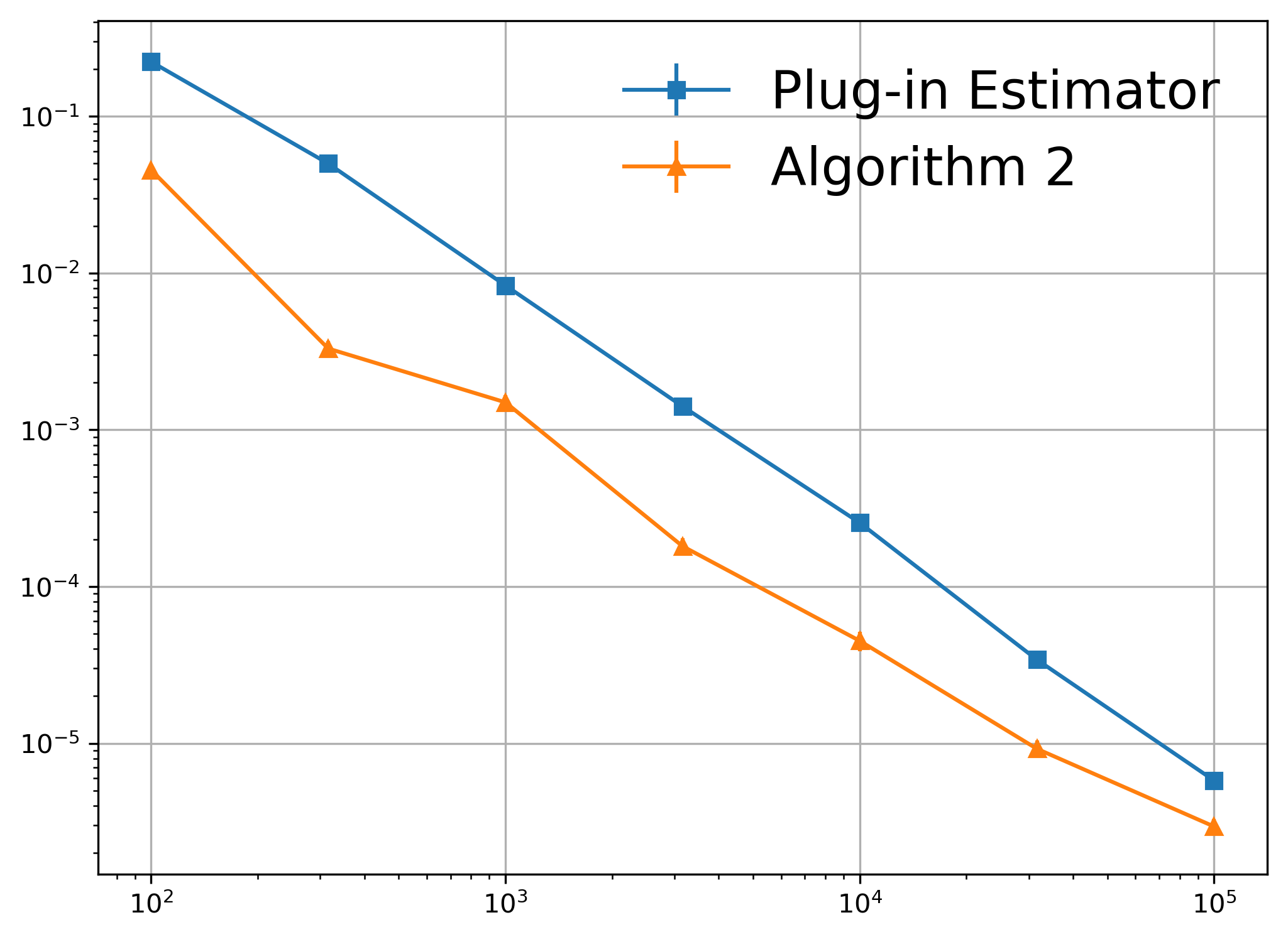
Figure 1: The proposed minimax optimal estimator in Algorithm 2 consistently improves upon the plug-in estimator on synthetic data.

3.2 Detecting violation of differential privacy with Algorithm 2

We demonstrate how we can use Algorithm 2 to detect mechanisms with false claim of DP guarantees on four types of mechanisms: Report Noisy Max [DR⁺14], Histogram [Dwo06], Sparse Vector Technique [LSL17] and Mixture of Truncated Geometric Mechanism. Following the experimental set-up of [DWW⁺18], the test query and databases defining $({\cal Q},{\cal D},{\cal D}^{\prime})$ are chosen by some heuristics, shown in Table 1. However, unlike the approach from [DWW⁺18], we do not require to know the size of the support $S$, we don’t have to specify candidate bad events $E\subseteq[S]$, and we can estimate general approximate DP with $\delta>0$. Throughout all the experiments, we fix $c_{1}=4$, $c_{2}=0.1$, $c_{3}=0.9$, and the mean of number of samples $n=100000$. For the examples in Report Noisy Max, Histogram, and Sparse Vector Technique, we compose 5 and 10 queries together to form a one giant query. There are several categories of queries and databases to be tested, each represented by the true answer of the 5 queries in the table. When testing, we test all categories, and report the largest estimate $\hat{\delta}$ for each given $\varepsilon$. For those faulty mechanisms, Algorithm 2 also provides a certificate in the form of a set $T\subseteq[S]$ such that $[P(T)-e^{\varepsilon}_{0}Q(T)]^{+}-\delta_{0}>0$.

Table 1: Database categories and samples [DWW⁺18]

Category	$[{\cal Q}_{1}({\cal D}),\ldots,{\cal Q}_{5}({\cal D})]$	$[{\cal Q}_{1}({\cal D}^{\prime}),\ldots,{\cal Q}_{5}({\cal D}^{\prime})]$
One Above	[1, 1, 1, 1, 1]	[2, 1, 1, 1, 1]
One Below	[1, 1, 1, 1, 1]	[0, 1, 1, 1, 1]
One Above Rest Below	[1, 1, 1, 1, 1]	[2, 0, 0, 0, 0]
One Below Rest Above	[1, 1, 1, 1, 1]	[0, 2, 2, 2, 2]
Half Half	[1, 1, 1, 1, 1]	[0, 0, 0, 2, 2]
All Above & All Below	[1, 1, 1, 1, 1]	[2, 2, 2, 2, 2]
X Shape	[1, 1, 1, 1, 1]	[0, 0, 1, 1, 1]

Report Noisy Max. For privacy budget $\varepsilon_{0}$, Report Noisy Argmax with Laplace noise (RNA+Lap) adds independent $Lap(2/\varepsilon_{0})$ noise to query answers ${\cal Q}({\cal D})$ and return the index of the largest noisy query answer. Report Noisy Argmax with Exponential noise (RNA+Exp) adds $Exp(2/\varepsilon_{0})$ noise instead of Laplace noise. Their claimed level of $(\varepsilon_{0})$-DP is correctly guaranteed [DR⁺14, Claim 3.9 and Theorem 3.10]. On the other hand, Report Noisy Max with Laplace noise (RNM+Lap) or Report Noisy Max with Exponential noise (RNM+Exp) return the largest noisy answer itself, instead of its index. This reveals more information than intended, leading to violation of claimed $(\varepsilon_{0},0)$-DP. Figure 2 shows $(\varepsilon,\delta)$ regions for the above variations of noisy max mechanisms. As expected, for each $\varepsilon_{0}$, RNA+Lap and RNA+Exp satisfy $(\varepsilon_{0},0)$-DP, whereas RNM+Lap and RNM+Exp have $\hat{\delta}>0$.

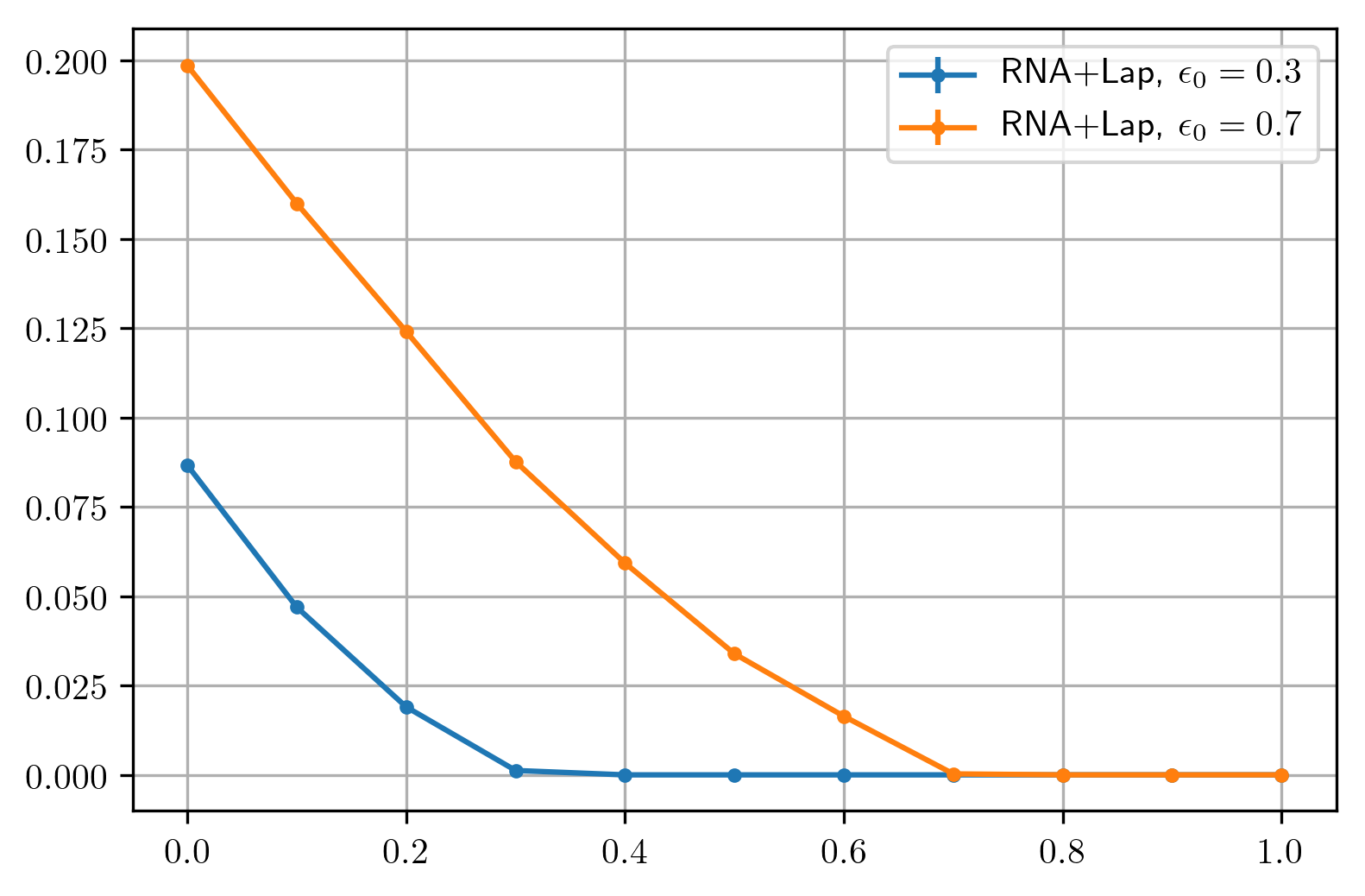
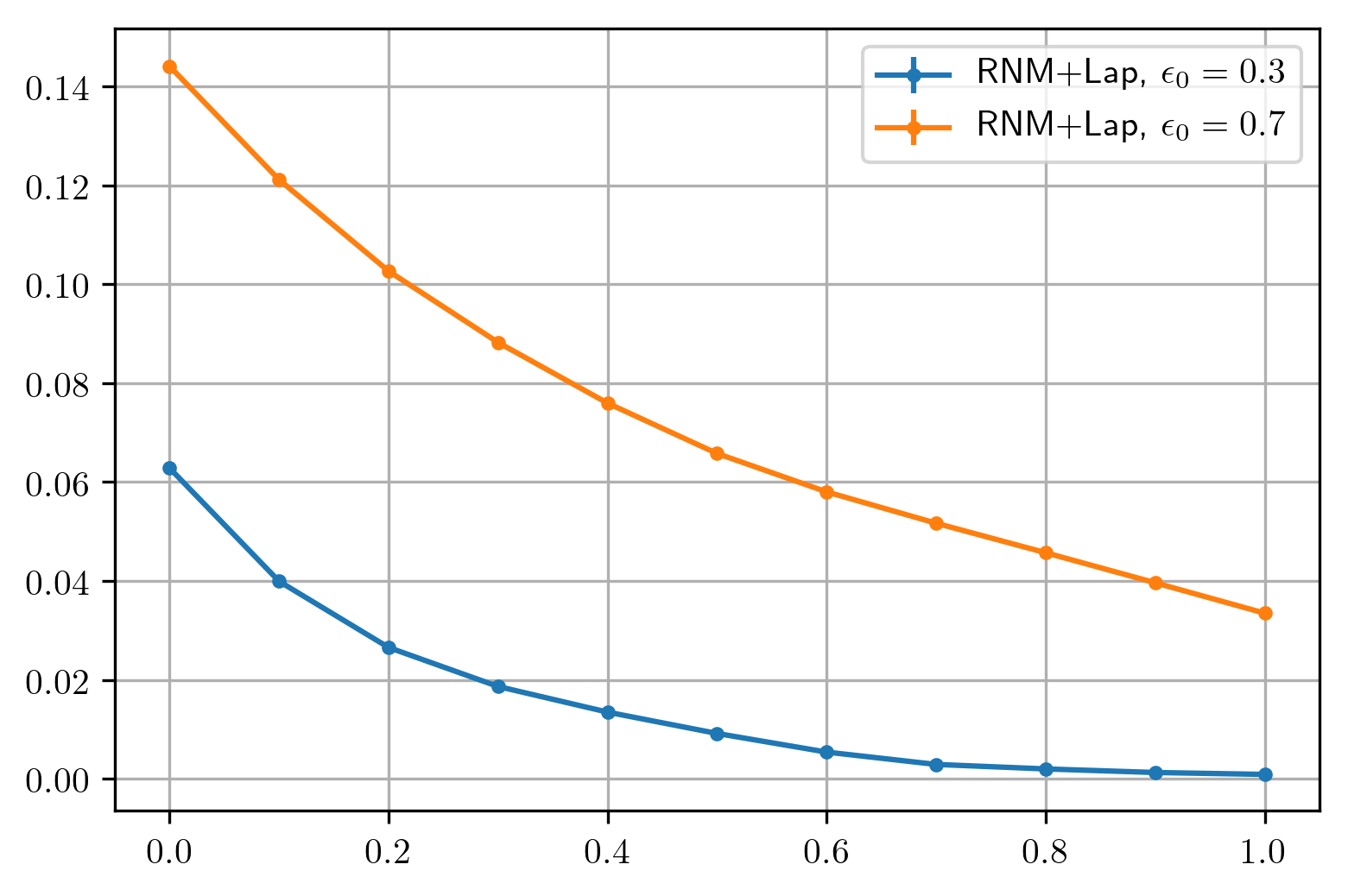
Figure 2: Estimate $\hat{\delta}$ from Algorithm 2 of $\delta$ given $\varepsilon$, and privacy budget $\varepsilon_{0}$ for noisy max mechanisms. Each point is showing an average over $10$ random trials with standard error.

Histogram. For privacy budget $\varepsilon_{0}$, Histogram takes histogram queries as input, adds independent $Lap(1/\varepsilon_{0})$ noise to each query answers, and output the randomized query answers directly, which is proved to be $(\varepsilon_{0},0)$-DP [DR⁺14]. As a comparison, Histogram with incorrect noise adds incorrect noise $Lap(\varepsilon_{0})$. Note that as we use histogram queries, we require ${\cal Q}({\cal D})$ and ${\cal Q}({\cal D}^{\prime})$ to be different in at most one element, which is tested on One Above and One Below samples as shown in Table 1. With the setting of privacy budget $\varepsilon_{0}=0.5$, Figure 3 left panel shows that the incorrect histogram is likely to be $(1/\varepsilon_{0},0)$-DP. Both mechanisms claim $(0.5,0)$-DP, but the figure shows that the incorrect mechanism ensures $(1/0.5,0)$-DP instead.

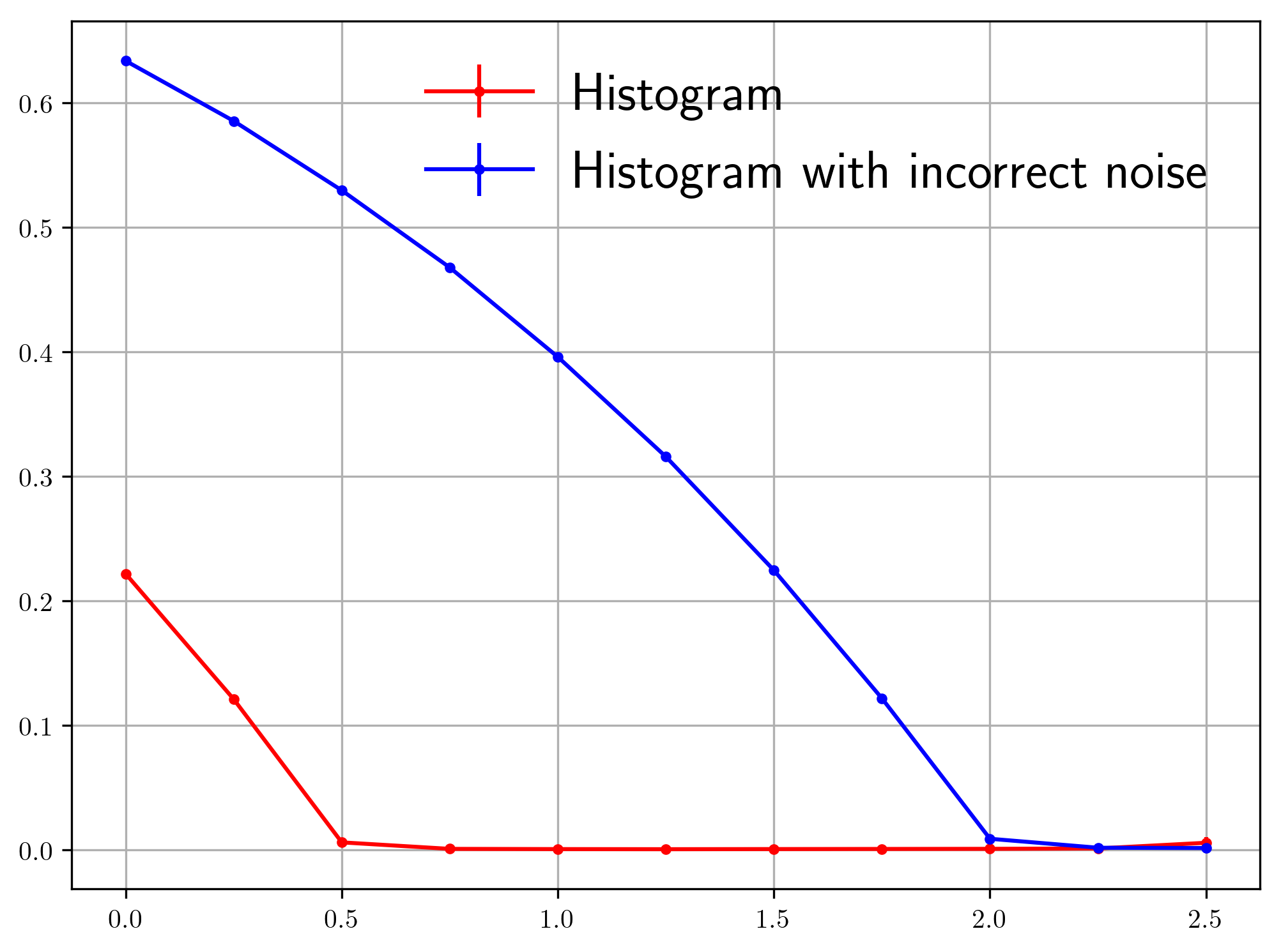
Figure 3: Estimates of $\delta$ given $\varepsilon$, and privacy budget $\varepsilon_{0}$ for histogram (left), SVT mechanisms (middle), Mixture of Truncated Geometric Mechanisms (right). Each point represents $10$ random trials with standard error bars.

Sparse Vector Technique (SVT). We consider original sparse vector technique mechanism SVT [LSL17], and its variations iSVT1 [SCM14], iSVT2 [CXZX15], and iSVT3 [LC14]. They are discussed in Section 1 and also studied and tested in [DWW⁺18]. With the setting of privacy budget $\varepsilon_{0}=0.5$, Figure 3 shows that SVT is likely to be $(\varepsilon_{0},0)$-DP. However, iSVT1 and iSVT2 are not likely to be pure differentially private for $\varepsilon\in[0,1]$ with budget $\varepsilon_{0}=0.5$. As discussed in [LSL17], iSVT3 is in fact $(\frac{(1+6N)}{4}\varepsilon_{0},0)$-DP, where $N$ is the bound of number of trues in the output Boolean vector and set as $N=1$ in this experiment. Figure 3 middle panel shows that with $\hat{\delta}=0$, $\varepsilon$ is likely to be in the range $[0.8,0.9]$, which verifies the theoretic guarantee.

Mixture of Truncated Geometric Mechanism (MTGM) With privacy budget $\varepsilon_{0}$, Truncated Geometric Mechanism (TGM) proposed by [GRS12] is provably to be $(\varepsilon_{0},0)$-DP. With probability privacy budget $\varepsilon_{0}$ and $\delta_{0}\in[0,1]$, Mixture of Truncated Geometric Mechanism (MTGM) outputs the original query answer with probability $\delta_{0}$, and outputs the randomized query answer with probability $1-\delta_{0}$. MTGM can be proved to be $(\varepsilon_{0},\delta_{0})$-DP by composition theorem. Note that TGM and MTGM both take single counting query as query function ${\cal Q}$. In the experiment, we consider the single counting query with range $\{0,1,2,3\}$. Figure 3 right panel confirms that MTGM satisfied the claimed $(\varepsilon_{0},\delta_{0})$ differential privacy.

4 Proof

4.1 Auxiliary lemmas

4.1.1 Lemmas on Poisson distribution

Lemma 2 ([MU05, Exercise 4.7]).

If $X\sim{\rm Poi}\,(\lambda)$, then for any $\delta>0$, we have

$${\mathbb{P}}\Big{(}X\geq(1+\delta)\lambda\Big{)} \;\;\leq\;\; \Big{(}\frac{e^{\delta}}{(1+\delta)^{1+\delta}}\Big{)}^{\lambda}\;\;\leq\;\;e^{-\delta^{2}\lambda/3}\;\vee\;e^{-\delta\lambda/3}\;,$$ (26)

$${\mathbb{P}}\Big{(}X\leq(1-\delta)\lambda\Big{)} \;\;\leq\;\; \Big{(}\frac{e^{-\delta}}{(1-\delta)^{1-\delta}}\Big{)}^{\lambda}\;\;\leq\;\;e^{-\delta^{2}\lambda/2}\;.$$ (27)

Lemma 3 ([MU05, Exercise 4.14]).

Suppose $X\sim{\rm Poi}\,(\lambda_{1})$, $Y\sim{\rm Poi}\,(\lambda_{2})$, and $Z=\alpha X+Y$, where $\alpha>1$ is a constant. Then $\mathbb{E}[Z]=\alpha\lambda_{1}+\lambda_{2}$, and for any $\delta>0$, we have

$${\mathbb{P}}\Big{(}Z\geq(1+\delta)(\alpha\lambda_{1}+\lambda_{2})\Big{)} \;\;\leq\;\; e^{-\delta^{2}(\alpha\lambda_{1}+\lambda_{2})/3}\vee e^{-\delta(\alpha\lambda_{1}+\lambda_{2})/3}\;,$$ (28)

$${\mathbb{P}}\Big{(}Z\leq(1-\delta)(\alpha\lambda_{1}+\lambda_{2})\Big{)} \;\;\leq\;\; e^{-\delta^{2}(\alpha\lambda_{1}+\lambda_{2})/2}\;.$$ (29)

Lemma 4.

Suppose $n{\hat{q}}\sim{\rm Poi}\,(nq)$, then

$$\mathbb{E}\big{[}\,[{\hat{q}}-q]^{+}\,\big{]}\;\in\;\left\{\begin{array}[]{rl}q\,e^{-nq}&\;,0\leq q\leq\frac{1}{n}\\ \Big{[}\,\sqrt{\frac{q}{4n}},\sqrt{\frac{q}{2n}}\,\Big{]}&\;,q\geq\frac{1}{n}\end{array}\right.$$ (32)

Hence,

$$\frac{1}{2}\Big{(}q\wedge\sqrt{\frac{q}{n}}\Big{)}\;\leq\;\mathbb{E}[[{\hat{q}}-q]^{+}]\;\leq\;\Big{(}q\wedge\sqrt{\frac{q}{n}}\Big{)}\;.$$ (33)

Proof.

Let $\lambda=nq$, then

$$\mathbb{E}\big{[}\,[{\hat{q}}-q]^{+}\,\big{]} = \frac{1}{n}\sum_{k=\lfloor\lambda\rfloor+1}^{\infty}\frac{\lambda^{k}e^{-\lambda}}{k!}(k-\lambda)$$

$$= \frac{1}{n}\sum_{k=\lfloor\lambda\rfloor+1}^{\infty}\frac{\lambda^{k}e^{-\lambda}}{k!}k\;-\;\frac{1}{n}\sum_{k=\lfloor\lambda\rfloor+1}^{\infty}\frac{\lambda^{k}e^{-\lambda}}{k!}\lambda$$

$$= \frac{1}{n}\lambda\sum_{k=\lfloor\lambda\rfloor}^{\infty}\frac{\lambda^{k}e^{-\lambda}}{k!}\;-\;\frac{1}{n}\lambda\sum_{k=\lfloor\lambda\rfloor+1}^{\infty}\frac{\lambda^{k}e^{-\lambda}}{k!}$$

$$= \frac{\lambda^{\lfloor\lambda\rfloor+1}e^{-\lambda}}{n\,\lfloor\lambda\rfloor!}$$

For $\lambda=nq\leq 1$, this is $qe^{-nq}$. For $\lambda\geq 1$, we use Stirling’s approximation to get

$$\frac{\lambda^{\lfloor\lambda\rfloor+1}e^{-\lambda}}{n\,\lfloor\lambda\rfloor!}\;\;\in\;\;\Big{[}\frac{1}{e},\frac{1}{\sqrt{2\pi}}\Big{]}\times\frac{\lambda^{\lfloor\lambda\rfloor+1}\,e^{-\lambda}}{n\,\lfloor\lambda\rfloor^{\lfloor\lambda\rfloor+\frac{1}{2}}\,e^{-\lfloor\lambda\rfloor}}\;.$$

As $\frac{\lambda^{\lfloor\lambda\rfloor+\frac{1}{2}}\,e^{-\lambda}}{\lfloor\lambda\rfloor^{\lfloor\lambda\rfloor+\frac{1}{2}}\,e^{-\lfloor\lambda\rfloor}}$ is in $[1\,,\,1.12]$ for $\lambda\geq 1$, this gives the desired bound. $\Box$

Lemma 5.

Suppose $n{\hat{q}}\sim{\rm Poi}\,(nq)$, then

$$\mathbb{E}\big{[}\,[p-e^{\varepsilon}{\hat{q}}]^{+}\,-\,[p-e^{\varepsilon}q]^{+}\big{]}\;\;\leq\;\;e^{\varepsilon}\,\min\,\Big{\{}\,q,e^{-\varepsilon}p,\sqrt{\frac{q}{n}},\sqrt{\frac{e^{-\varepsilon}p}{n}}\,\Big{\}}\;.$$ (34)

Proof.

$$\mathbb{E}\big{[}\,[p-e^{\varepsilon}{\hat{q}}]^{+}-[p-e^{\varepsilon}q]^{+}\,\big{]} = \mathbb{E}\big{[}\,\frac{(p-e^{\varepsilon}{\hat{q}})+|p-e^{\varepsilon}{\hat{q}}|}{2}-\frac{(p-e^{\varepsilon}q)+|p-e^{\varepsilon}q|}{2}\,\big{]}$$

$$= \frac{1}{2}\,\Big{(}\mathbb{E}\big{[}\,|p-e^{\varepsilon}{\hat{q}}|\,\big{]}-|p-e^{\varepsilon}q|\Big{)}\;.$$

If $p\geq e^{\varepsilon}q$, then

$$\frac{1}{2}\,\Big{(}\mathbb{E}\big{[}\,|p-e^{\varepsilon}{\hat{q}}|\,\big{]}-|p-e^{\varepsilon}q|\Big{)} = \frac{1}{2}\,\Big{(}\mathbb{E}\big{[}\,|p-e^{\varepsilon}{\hat{q}}|-(p-e^{\varepsilon}q)\,\big{]}\Big{)}$$

$$= \frac{1}{2}\,\Big{(}\mathbb{E}\big{[}\,(p-e^{\varepsilon}{\hat{q}})-(p-e^{\varepsilon}q)+2[e^{\varepsilon}{\hat{q}}-p]^{+}\,\big{]}\Big{)}$$

$$= \mathbb{E}\big{[}\,[e^{\varepsilon}{\hat{q}}-p]^{+}\,\big{]}$$

$$\leq e^{\varepsilon}\mathbb{E}\big{[}\,[{\hat{q}}-q]^{+}\,\big{]}$$

$$\leq e^{\varepsilon}\Big{(}q\wedge\sqrt{\frac{q}{n}}\Big{)}\;,$$

where the second equality is because of the fact that $x=[x]^{+}-[-x]^{+}$ and $|x|=[x]^{+}+[-x]^{+}$, the first inequality follows from the fact that $[x]^{+}$ is monotone, and the last inequality follows from Lemma 4.

If $p<e^{\varepsilon}q$, then

$$\frac{1}{2}\,\Big{(}\mathbb{E}\big{[}\,|p-e^{\varepsilon}{\hat{q}}|\,\big{]}-|p-e^{\varepsilon}q|\Big{)} = \frac{1}{2}\,\Big{(}\mathbb{E}\big{[}\,|p-e^{\varepsilon}{\hat{q}}|-(e^{\varepsilon}q-p)\,\big{]}\Big{)}$$

$$= \frac{1}{2}\,\Big{(}\mathbb{E}\big{[}\,(e^{\varepsilon}{\hat{q}}-p)-(e^{\varepsilon}q-p)+2[p-e^{\varepsilon}{\hat{q}}]^{+}\,\big{]}\Big{)}$$

$$= \mathbb{E}\big{[}\,[p-e^{\varepsilon}{\hat{q}}]^{+}\,\big{]}\;,$$

Now we construct new random variable ${\hat{p}}$ by $n{\hat{q}}=ne^{-\varepsilon}{\hat{p}}+Z$, where $Z$ is independent of ${\hat{p}}$ and $Z\sim{\rm Poi}\,(n(q-e^{-\varepsilon}p))$. Hence, $e^{-\varepsilon}{\hat{p}}\leq{\hat{q}}$ with probability one. And the marginal distribution satisfies $ne^{-\varepsilon}{\hat{p}}\sim{\rm Poi}\,(ne^{-\varepsilon}p)$. We have

$$\mathbb{E}\big{[}\,[e^{-\varepsilon}p-{\hat{q}}]^{+}\,\big{]} \leq \mathbb{E}\big{[}\,[e^{-\varepsilon}p-e^{-\varepsilon}{\hat{p}}]^{+}\,\big{]}$$

$$\leq \Big{(}e^{-\varepsilon}p\wedge\sqrt{\frac{e^{-\varepsilon}p}{n}}\Big{)}\;,$$

where the first inequality follows from that fact that $[x]^{+}$ is monotone, and the last inequality follows from Lemma 4. $\Box$

Lemma 6.

Suppose $n{\hat{q}}\sim{\rm Poi}\,(nq)$, then for any $p$ and $q$, we have

$${\rm Var}\big{(}\,[p-e^{\varepsilon}\,{\hat{q}}]^{+}\,\big{)} \;\;\lesssim\;\; \frac{e^{\varepsilon}p}{n}\;.$$ (35)

Proof.

Case 1: If $nq<1$ and $e^{-\varepsilon}p\geq q$ or if $nq\geq 1$ and $ne^{-\varepsilon}p>\lfloor nq\rfloor-1$:

$${\rm Var}\big{(}\,[p-e^{\varepsilon}{\hat{q}}]^{+}\,\big{)} \;\;=\;\; \inf_{a}\mathbb{E}\big{(}\,[p-e^{\varepsilon}{\hat{q}}]^{+}-a\,\big{)}^{2}$$

$$\;\;\leq\;\; \mathbb{E}\big{(}\,[p-e^{\varepsilon}{\hat{q}}]^{+}-[p-e^{\varepsilon}q]^{+}\,\big{)}^{2}$$

$$\;\;=\;\; \mathbb{E}\big{(}\,\frac{(p-e^{\varepsilon}{\hat{q}})-(p-e^{\varepsilon}q)}{2}+\frac{|p-e^{\varepsilon}{\hat{q}}|-|p-e^{\varepsilon}q|}{2}\,\big{)}^{2}$$

$$\;\;\leq\;\; \mathbb{E}\big{(}\,\frac{e^{\varepsilon}|{\hat{q}}-q|}{2}+\frac{\big{|}|p-e^{\varepsilon}{\hat{q}}|-|p-e^{\varepsilon}q|\big{|}}{2}\,\big{)}^{2}$$

$$\;\;\leq\;\; e^{2\varepsilon}\mathbb{E}\big{(}\,\frac{|{\hat{q}}-q|}{2}+\frac{|{\hat{q}}-q|}{2}\,\big{)}^{2}$$

$$\;\;=\;\; e^{2\varepsilon}\mathbb{E}\big{(}\,{\hat{q}}-q\,\big{)}^{2}$$

$$\;\;=\;\; \frac{e^{2\varepsilon}q}{n}$$

$$\;\;\leq\;\; \frac{e^{\varepsilon}p}{n}\;,$$

where the last step follows from the assumption that $e^{-\varepsilon}p\geq q$.

Case 2: If $nq<1$ and $e^{-\varepsilon}p<q$ or if $nq\geq 1$ and $ne^{-\varepsilon}p<1$ :

In both cases, $ne^{-\varepsilon}p<1$, and we have

$$[ne^{-\varepsilon}p-n{\hat{q}}]^{+}=\left\{\begin{array}[]{ll}ne^{-\varepsilon}p&\text{w.p.}\quad e^{-nq}\\ 0&\text{w.p.}\quad 1-e^{-nq}\\ \end{array}\right.\;,$$

which is a Bernoulli random variable. The variance of it is

$${\rm Var}\,\big{(}[p-e^{\varepsilon}{\hat{q}}]^{+}\big{)} \;\;=\;\; \frac{e^{2\varepsilon}}{n^{2}}{\rm Var}\,\big{(}[ne^{-\varepsilon}p-n{\hat{q}}]^{+}\big{)}$$

$$\;\;=\;\; p^{2}(1-e^{-nq})e^{-nq}$$

$$\;\;\leq\;\; p^{2}\;\;<\;\;\frac{e^{\varepsilon}p}{n}\;,$$

where we used the assumption that $ne^{-\varepsilon}p<1$.

Case 3: If $nq\geq 1$ and $1\leq ne^{-\varepsilon}p\leq\lfloor nq\rfloor-1$:

Let $\lambda=nq$, and denote the random variable $X\sim{\rm Poi}\,(\lambda)$.

If $1\leq ne^{-\varepsilon}p\leq\lfloor nq\rfloor-1$, we know from Lemma 2 that

$${\mathbb{P}}\big{(}X\leq ne^{-\varepsilon}p\big{)}\;\;\leq\;\;e^{-D_{\rm KL}(ne^{-\varepsilon}p\|nq)}\;,$$ (37)

where $D_{\rm KL}(k\|m)\triangleq m-k+k\ln(k/m)$.

We have

$$\mathbb{E}\big{(}\,[p-e^{\varepsilon}{\hat{q}}]^{+}\,\big{)}^{2} \;\;=\;\; \sum_{k=0}^{\lfloor ne^{-\varepsilon}p\rfloor}\Big{(}p-e^{\varepsilon}\frac{k}{n}\Big{)}^{2}\Big{(}\frac{\lambda^{k}e^{-\lambda}}{k!}\Big{)}$$

$$\;\;=\;\; p^{2}{\mathbb{P}}\big{(}X\leq ne^{-\varepsilon}p\big{)}-2e^{\varepsilon}pq{\mathbb{P}}\big{(}X\leq ne^{-\varepsilon}p-1\big{)}$$

$$+\frac{e^{2\varepsilon}q}{n}{\mathbb{P}}\big{(}X\leq ne^{-\varepsilon}p-1\big{)}+e^{2\varepsilon}q^{2}{\mathbb{P}}\big{(}X\leq ne^{-\varepsilon}p-2\big{)}$$

$$\;\;=\;\; p^{2}{\mathbb{P}}\big{(}X\leq ne^{-\varepsilon}p\big{)}-2e^{\varepsilon}pq{\mathbb{P}}\big{(}X\leq ne^{-\varepsilon}p\big{)}+2e^{\varepsilon}pq{\mathbb{P}}\big{(}X=\lfloor ne^{-\varepsilon}p\rfloor\big{)}$$

$$+\frac{e^{2\varepsilon}q}{n}{\mathbb{P}}\big{(}X\leq ne^{-\varepsilon}p\big{)}-\frac{e^{2\varepsilon}q}{n}{\mathbb{P}}\big{(}X=\lfloor ne^{-\varepsilon}p\rfloor\big{)}$$

$$+e^{2\varepsilon}q^{2}{\mathbb{P}}\big{(}X\leq ne^{-\varepsilon}p\big{)}-e^{2\varepsilon}q^{2}{\mathbb{P}}\big{(}X=\lfloor ne^{-\varepsilon}p\rfloor\big{)}-e^{2\varepsilon}q^{2}{\mathbb{P}}\big{(}X=\lfloor ne^{-\varepsilon}p\rfloor-1\big{)}$$

$$\;\;=\;\; (p^{2}-2e^{\varepsilon}pq+\frac{e^{2\varepsilon}q}{n}+e^{2\varepsilon}q^{2}){\mathbb{P}}\big{(}X\leq ne^{-\varepsilon}p\big{)}$$

$$+(2e^{\varepsilon}pq-\frac{e^{2\varepsilon}q}{n}-e^{2\varepsilon}q^{2}-\frac{e^{2\varepsilon}q\lfloor ne^{-\varepsilon}p\rfloor}{n}){\mathbb{P}}\big{(}X=\lfloor ne^{-\varepsilon}p\rfloor\big{)}$$

$$\;\;\lesssim\;\; \Big{(}(e^{\varepsilon}q-p)^{2}\vee\frac{e^{2\varepsilon}q}{n}\Big{)}e^{-D_{\rm KL}(ne^{-\varepsilon}p\|nq)}\;.$$

Let $y=q/(e^{-\varepsilon}p)$, as $1\leq ne^{-\varepsilon}p\leq\lfloor nq\rfloor-1$, we know $y>1$.

We have

$$\frac{e^{2\varepsilon}q}{n}e^{-D_{\rm KL}(ne^{-\varepsilon}p\|nq)} \;\;=\;\; \frac{e^{\varepsilon}py}{n}e^{-ne^{-\varepsilon}p(y-1-\ln y)}$$

$$\;\;\lesssim\;\; \frac{e^{\varepsilon}p}{n}\;,$$

where we used the assumption that $ne^{-\varepsilon}p\geq 1$ and the inequality that $ye^{-(y-1-\ln y)}$ is bounded by some constant for $y>1$.

We have

$$(e^{\varepsilon}q-p)^{2}e^{-D_{\rm KL}(ne^{-\varepsilon}p\|nq)} \;\;=\;\; (y-1)^{2}p^{2}e^{-ne^{-\varepsilon}p(y-1-\ln y)}$$

$$\;\;\lesssim\;\; \frac{e^{\varepsilon}p}{n}\;,$$

where we used the assumption that $ne^{-\varepsilon}p\geq 1$ and the inequality that $(y-1)^{2}e^{-x(y-1-\ln y)}\lesssim 1/x$ for $x,y>1$.

It suffices to show that $f_{y}(x)=\ln x-x(y-1-\ln y)+2\ln(y-1)$ is bounded by some constant for $x,y>1$. Indeed, when $y-1-\ln y>1$, $f_{y}^{\prime}(x)=1/x-(y-1-\ln y)<0$. $f_{y}(x)$ is monotonically decreasing and $f_{y}(x)<f_{y}(1)=2\ln(y-1)-y+1+\ln y$, which is bounded. When $y-1-\ln y<1$, $f_{y}(x)$ attains maximum at $x=1/(y-1-\ln y)$. In this case, we have $f_{y}(x)\leq 2\ln(y-1)-\ln(y-1-\ln y)-1$, which is also bounded.

$\Box$

Lemma 7.

Suppose $n{\hat{q}}\sim{\rm Poi}\,(nq)$. Then,

$${\mathbb{P}}\left(e^{\varepsilon}{\hat{q}}\notin U(e^{2\varepsilon}q;c_{1},c_{1})\right)\;\;\leq\;\;\frac{2}{n^{-c_{1}e^{-\varepsilon}/3}}\;\;\leq\;\;\frac{2}{n^{-c_{1}/3}}\;,$$ (38)

and

$${\mathbb{P}}\left({\hat{q}}\notin U(e^{\varepsilon}q;c_{1},c_{1})\right)\;\;\leq\;\;\frac{2}{n^{-c_{1}/3}}\;.$$ (39)

Proof.

The second inequality is exactly [JHW18, Lemma 1]. We now prove the first inequality.

If $q\leq\frac{c_{1}e^{-\varepsilon}\ln n}{n}$, we have

$${\mathbb{P}}\left(e^{\varepsilon}{\hat{q}}\notin U(e^{2\varepsilon}q:c_{1},c_{1})\right) \;\;=\;\; {\mathbb{P}}\left(n{\hat{q}}\geq 2c_{1}e^{-\varepsilon}\ln n\right)$$

$$\;\;\leq\;\; {\mathbb{P}}\left({\rm Poi}\,(c_{1}e^{-\varepsilon}\ln n)\geq 2c_{1}e^{-\varepsilon}\ln n\right)$$

$$\;\;\leq\;\; e^{-\frac{c_{1}e^{-\varepsilon}\ln n}{3}}\;,$$

where we applied Lemma 2 in the last inequality.

If $q>\frac{c_{1}e^{-\varepsilon}\ln n}{n}$, we have

$${\mathbb{P}}\left(e^{\varepsilon}{\hat{q}}\notin U(e^{2\varepsilon}q;c_{1},c_{1})\right) \;\;=\;\; {\mathbb{P}}\left(e^{\varepsilon}{\hat{q}}>e^{\varepsilon}q+\sqrt{\frac{c_{1}e^{\varepsilon}q\ln n}{n}}\right)+{\mathbb{P}}\left(e^{\varepsilon}{\hat{q}}<e^{\varepsilon}q-\sqrt{\frac{c_{1}e^{\varepsilon}q\ln n}{n}}\right)$$

$$\;\;\leq\;\; {\mathbb{P}}\left({\rm Poi}\,(nq)>nq+\sqrt{c_{1}qe^{-\varepsilon}n\ln n}\right)+{\mathbb{P}}\left({\rm Poi}\,(nq)<nq-\sqrt{c_{1}qe^{-\varepsilon}n\ln n}\right)$$

$$\;\;\leq\;\; e^{-\frac{c_{1}e^{-\varepsilon}\ln n}{nq}\frac{nq}{3}}+e^{-\frac{c_{1}e^{-\varepsilon}\ln n}{nq}\frac{nq}{2}}$$

$$\;\;\leq\;\; \frac{2}{n^{c_{1}e^{-\varepsilon}/3}}\;.$$

$\Box$

4.1.2 Lemmas on the best polynomial approximation

The first-order and second-order symmetric difference with function $\varphi(x)=\sqrt{x(1-x)}$ are defined as

$$\Delta_{h\varphi}f(x)\;\;\triangleq\;\;f(x+\frac{h\varphi(x)}{2})-f(x-\frac{h\varphi(x)}{2})\;,$$ (40)

and

$$\Delta_{h\varphi}^{2}f(x)\;\;=\;\;f(x+h\varphi(x))-2f(x)+f(x-h\varphi(x))\;,$$ (41)

respectively.

For function $f(x)$ with domain $[0,1]$, the first-order Ditzian-Totik modulus of smoothness is defined as

$$\omega_{\varphi}^{1}(f,t)\;\;\triangleq\;\;\sup_{0<h\leq t}\|\Delta_{h\varphi}^{1}f(x)\|_{\infty}\;,$$ (42)

and the second-order Ditzian-Totik modulus of smoothness is defined as

$$\omega_{\varphi}^{2}(f,t)\;\;\triangleq\;\;\sup_{0<h\leq t}\|\Delta_{h\varphi}^{2}f(x)\|_{\infty}\;.$$ (43)

The following lemma upper bounds the best polynomial approximation error by the Ditzian-Totik moduli.

Lemma 8 ([Dit87, Theorem 7.2.1 and 12.1.1]).

There exists a constant $M(r)>0$ such that for any function $f\in C[0,1]$,

$$\Delta_{L}[f;[0,1]]\;\;\leq\;\;M(r)\omega_{\varphi}^{r}(f,\frac{1}{L})\;,\quad L>r\;,$$ (44)

where $\Delta_{L}[f;I]$ denotes the distance of the function $f$ to the space ${\rm poly_{L}}$ in the uniform norm $\|\cdot\|_{\infty},I$ on $I\subset{\mathbb{R}}$. Moreover, if $f(x):[0,1]^{2}\mapsto{\mathbb{R}}$, we have

$$\Delta_{L}[f;[0,1]^{2}]\;\;\leq\;\;M\omega_{[0,1]^{2}}^{r}(f,\frac{1}{L})\;,\quad L>r\;,$$ (45)

where $M$ is independent of $f$ and $L$, and $\Delta_{L}[f;[0,1]^{2}]$ denotes the distance of the function $f$ to the space ${\rm poly_{L}^{2}}$ in the uniform norm on $[0,1]^{2}$.

Lemma 9.

For $f(x)=[p-e^{\varepsilon}2x\Delta]^{+}$, for some $\Delta>0$, $p\in[0,2e^{\varepsilon}\Delta]$, $x\in[0,1]$, and any integer $K\geq 1$,

$$\omega_{\varphi}^{2}(f,K^{-1})\;\;=\;\;\left\{\begin{array}[]{ll}p&\frac{p}{2e^{\varepsilon}\Delta}\leq\frac{1}{1+K^{2}}\\ \frac{\sqrt{p(2e^{\varepsilon}\Delta-p)}}{K}&\frac{1}{1+K^{2}}\leq\frac{p}{2e^{\varepsilon}\Delta}\leq\frac{K^{2}}{1+K^{2}}\\ e^{\varepsilon}\Delta-p&\frac{K^{2}}{1+K^{2}}\leq\frac{p}{2e^{\varepsilon}\Delta}\leq 1\end{array}\right.\;\;\lesssim\;\;\min\Big{\{}p\;,\frac{\sqrt{p(2e^{\varepsilon}\Delta-p)}}{K}\;,e^{\varepsilon}\Delta-p\Big{\}}\;,$$

where $\omega_{\varphi}^{2}(f,t)$ is defined in Eq. (43).

Proof.

Let $g(x):=|p-2e^{\varepsilon}\Delta x|$.

$$\Delta_{h\varphi}^{2}f(x) = [p-2e^{\varepsilon}\Delta(x+h\varphi(x))]^{+}-2[p-2e^{\varepsilon}\Delta x]^{+}+[p-2e^{\varepsilon}\Delta(x-h\varphi(x))]^{+}$$

$$= \frac{\big{(}p-2e^{\varepsilon}\Delta(x+h\varphi(x))\big{)}-2\big{(}p-2e^{\varepsilon}\Delta x\big{)}+\big{(}p-2e^{\varepsilon}\Delta(x-h\varphi(x))\big{)}}{2}+$$

$$\frac{\big{|}p-2e^{\varepsilon}\Delta(x+h\varphi(x))\big{|}-2\big{|}p-2e^{\varepsilon}\Delta x\big{|}+\big{|}p-2e^{\varepsilon}\Delta(x-h\varphi(x))\big{|}}{2}$$

$$= \frac{1}{2}\Delta_{h\varphi}^{2}g(x)$$

Hence,

$$\omega_{\varphi}^{2}(f,t)=\frac{1}{2}\omega_{\varphi}^{2}(g,t)$$ (47)

It follows from [JHW18, Lemma 12] that, for some $\Delta>0$, $p\in[0,2e^{\varepsilon}\Delta]$, $x\in[0,1]$ and any integer $K\geq 1$, we have:

$$\omega_{\varphi}^{2}(g,K^{-1})\;\;=\;\;\left\{\begin{array}[]{ll}2p&\frac{p}{2e^{\varepsilon}\Delta}\leq\frac{1}{1+K^{2}}\\ \frac{2\sqrt{p(2e^{\varepsilon}\Delta-p)}}{K}&\frac{1}{1+K^{2}}\leq\frac{p}{2e^{\varepsilon}\Delta}\leq\frac{K^{2}}{1+K^{2}}\\ 2e^{\varepsilon}\Delta-p&\frac{K^{2}}{1+K^{2}}\leq\frac{p}{2e^{\varepsilon}\Delta}\leq 1\end{array}\right.\;\;,$$

which implies the desired bound.

$\Box$

Lemma 10.

Suppose $f(x)=[\sqrt{x}-\sqrt{a}]^{+}$, $x\in[0,1]$ and $a\in[0,1]$. Then

$$\omega_{\varphi}^{1}(f,t)\;\;\leq\;\;\frac{t}{\sqrt{2}}\;.$$ (49)

Similarly, suppose $f(x)=[\sqrt{a}-\sqrt{x}]^{+}$, $x\in[0,1]$ and $a\in[0,1]$. Then

$$\omega_{\varphi}^{1}(f,t)\;\;\leq\;\;\frac{t}{\sqrt{2}}\;.$$ (50)

Proof.

Let $g(x)=|\sqrt{x}-\sqrt{a}|$.

$$\Delta^{1}_{h\varphi}f(x) \;\;=\;\; \left|f(x+\frac{h\varphi(x)}{2})-f(x-\frac{h\varphi(x)}{2})\right|$$

$$\;\;=\;\; \left|\left[\sqrt{x+\frac{h\varphi(x)}{2}}-\sqrt{a}\right]^{+}-\left[\sqrt{x-\frac{h\varphi(x)}{2}}-\sqrt{a}\right]^{+}\right|$$

$$\;\;=\;\; \left|\frac{1}{2}\left(\left|\sqrt{x+\frac{h\varphi(x)}{2}}-\sqrt{a}\right|-\left|\sqrt{x-\frac{h\varphi(x)}{2}}-\sqrt{a}\right|\right)+\right.$$

$$\left.\frac{\sqrt{x+\frac{h\varphi(x)}{2}}-\sqrt{x-\frac{h\varphi(x)}{2}}}{2}\right|$$

$$\;\;\leq\;\; \frac{1}{2}\nabla^{1}_{h\varphi}g(x)+\frac{1}{2}\left|\sqrt{x+\frac{h\varphi(x)}{2}}-\sqrt{x-\frac{h\varphi(x)}{2}}\right|$$

$$\;\;=\;\; \frac{1}{2}\nabla^{1}_{h\varphi}g(x)+\frac{1}{2}\left|\frac{h\varphi(x)}{\sqrt{x+h\varphi(x)/2}+\sqrt{x-h\varphi(x)/2}}\right|$$

$$\;\;\leq\;\; \frac{1}{2}\nabla^{1}_{h\varphi}g(x)+\frac{1}{2}\left|\frac{h\varphi(x)}{\sqrt{x+h\varphi(x)/2+x-h\varphi(x)/2}}\right|$$

$$\;\;\leq\;\; \frac{1}{2}\nabla^{1}_{h\varphi}g(x)+\frac{h\sqrt{1-x}}{2\sqrt{2}}$$

$$\;\;\leq\;\; \frac{t}{\sqrt{2}}\;,$$

where we used the fact that $\sqrt{x}+\sqrt{y}\leq x+y$ and [JHW18, Lemma 11] for smoothness of $g$. $\Box$

Lemma 11 ([HJW16, Lemma 27]).

Let $p_{n}(x)=\sum_{v=0}^{n}a_{v}x^{v}$ be a polynomial of degree at most $n$ such that $|p_{n}(x)|\leq A$ for $x\in[a,b]$. Then

1. If $a+b\neq 0$, then

   $$|a_{v}|\;\;\leq\;\;2^{7n/2}A\left|\frac{a+b}{2}\right|^{-v}\left(\left|\frac{b+a}{b-a}\right|^{n}+1\right)\;,\qquad v=0,1,\cdots,n\;.$$ (51)

2. If $a+b=0$, then

   $$|a_{v}|\;\;\leq\;\;Ab^{-v}(\sqrt{(}2)+1)^{n}\;,\qquad v=0,1,\cdots,n\;.$$ (52)

4.1.3 Lemmas on the uniformly unbiased minimum variance unbiased estimator

Lemma 12 ([JHW18, Lemma 18]).

Suppose $nX\sim{\rm Poi}\,(np)$, $p\geq 0$, $q\geq 0$. Then, the estimator

$$g_{j,q}(X)\triangleq\sum_{k=0}^{j}{j\choose k}(-q)^{j-k}\prod_{h=0}^{k-1}\left(X-\frac{h}{n}\right)$$ (53)

is the unique uniformly minimum variance unbiased estimator for $(p-q)^{j}$, $j\geq 0$, $j\in\mathbb{N}$, and its second moment is given by

$$\mathbb{E}\left[\big{(}g_{j,q}(X)\big{)}^{2}\right]\;\;=\;\;\sum_{k=0}^{j}{j\choose k}^{2}(p-q)^{2(j-k)}\frac{p^{k}k!}{n^{k}}\;\;=\;\;j!\left(\frac{p}{n}\right)^{j}L_{j}\left(-\frac{n(p-q)^{2}}{p}\right)\text{assuming $p>0$}\;,$$ (54)

where $L_{m}(x)$ stands for the Laguerre polynomial with order $m$, which is defined as:

$$L_{m}(x)\;\;=\;\;\sum_{k=0}^{m}{m\choose k}\frac{(-x)^{k}}{k!}\;.$$ (55)

If $M\geq\max\left\{\frac{n(p-q)^{2}}{p},j\right\}$, we have

$$\mathbb{E}\left[\big{(}g_{j,q}(X)\big{)}^{2}\right]\;\;\leq\;\;\left(\frac{2Mp}{n}\right)^{j}\;.$$ (56)

When $k=0$, $\prod_{h=0}^{k-1}\left(X-\frac{h}{n}\right)\triangleq 1$. When $p=0$, $g_{j,q}(X)\equiv(-q)^{j}$, $\mathbb{E}\left[g_{j,q}(X)\right]^{2}\equiv q^{2j}$.

Lemma 13.

Suppose $(n{\hat{p}},n{\hat{q}})\sim{\rm Poi}\,(np)\times{\rm Poi}\,(nq)$. Then the following estimator using $({\hat{p}},{\hat{q}})$ is the unique uniformly minimum unbiased estimator for $(e^{\varepsilon}q-p)^{j}$, $j\geq 0$, $j\in\mathbb{Z}$:

$$\hat{A}_{j}({\hat{p}},{\hat{q}})\;\;=\;\;\sum_{k=0}^{j}{j\choose k}\prod_{i=0}^{k-1}\left({\hat{q}}-\frac{i}{n}\right)e^{\varepsilon k}(-1)^{j-k}\prod_{m=0}^{j-k}\left({\hat{p}}-\frac{m}{n}\right)\;.$$ (57)

Furthermore,

$$\mathbb{E}\hat{A}_{j}^{2}\;\;\leq\;\;\left(2(e^{\varepsilon}q-p)^{2}\vee\frac{8j(e^{2\varepsilon}q\vee p)}{n}\right)^{j}\;.$$ (58)

Proof.

It follows from [JHW18, Lemma 19] and binomial theorem that $\hat{A}_{j}({\hat{p}},{\hat{q}})$ is the unique uniformly minimum variance unbiased estimator for $(e^{\varepsilon}q-p)^{j}$. Now we show $\mathbb{E}\hat{A}_{j}^{2}$ is bounded.

It follows from binomial theorem again that for any fixed $r>0$,

$$(e^{\varepsilon}q-p)^{j} \;\;=\;\; (e^{\varepsilon}q-r+r-p)^{j}$$ (59)

$$\;\;=\;\; \sum_{k=0}^{j}{j\choose k}(e^{\varepsilon}q-r)^{k}(-1)^{j-k}(p-r)^{j-k}\;.$$ (60)

The following estimator is also unbiased for estimating $(e^{\varepsilon}q-p)^{j}$,

$$\sum_{k=0}^{j}e^{\varepsilon k}g_{k,\frac{r}{e^{\varepsilon}}}({\hat{q}})(-1)^{j-k}g_{j-k,r}({\hat{p}})\;,$$ (61)

where $g_{i,q}({\hat{p}})$ is defined in Lemma 12.

Define $M_{1}=\frac{n(q-\frac{r}{e^{\varepsilon}})^{2}}{p}\vee j$, $M_{2}=\frac{n(p-r)^{2}}{p}\vee j$, $M=2(e^{\varepsilon}q-p)^{2}\vee\frac{8j(e^{2\varepsilon}q\vee p)}{n}$ and set $r=\frac{e^{\varepsilon}q+p}{2}$.

Denote $\|X\|_{2}=\sqrt{\mathbb{E}(X-\mathbb{E}X)^{2}}$ for random variable $X$. It follows from Lemma 12 that

$$\|\hat{A}_{j}\|_{2} \;\;\leq\;\; \sum_{k=0}^{j}{j\choose k}e^{\varepsilon k}\|g_{k,\frac{r}{e^{\varepsilon}}}({\hat{q}})\|_{2}\cdot\|g_{j-k,r}({\hat{p}})\|_{2}$$

$$\;\;\leq\;\; \sum_{k=0}^{j}{j\choose k}e^{\varepsilon k}\left(\frac{2M_{1}q}{n}\right)^{k/2}\left(\frac{2M_{2}p}{n}\right)^{(j-k)/2}$$

$$\;\;=\;\; \left(e^{\varepsilon}\sqrt{\frac{2M_{1}q}{n}}+\sqrt{\frac{2M_{2}p}{n}}\right)^{j}$$

$$\;\;=\;\; \left(\sqrt{\frac{(e^{\varepsilon}q-p)^{2}}{2}\vee\frac{2je^{2\varepsilon}q}{n}}+\sqrt{\frac{(e^{\varepsilon}q-p)^{2}}{2}\vee\frac{2jp}{n}}\right)^{j}$$

$$\;\;=\;\; M^{j/2}\;.$$

$\Box$

4.2 Proof of Theorem 1

Note that

$$\mathbb{E}_{Q}\big{[}\,|d_{\varepsilon}(P\|Q_{n})-d_{\varepsilon}(P\|Q)|^{2}\,\big{]}\;\;=\;\;\Big{(}\sum_{i=1}^{S}\mathbb{E}_{Q}\big{[}\,[p_{i}-e^{\varepsilon}{\hat{q}}_{i}]^{+}\big{]}-[p_{i}-e^{\varepsilon}q_{i}]^{+}\Big{)}^{2}+{\rm Var}\big{(}d_{\varepsilon}(P\|Q_{n})\big{)}\;.$$ (62)

We first claim the following upper bound for all $P$:

$$\sum_{i=1}^{S}\mathbb{E}_{Q}\big{[}\,[p_{i}-e^{\varepsilon}{\hat{q}}_{i}]^{+}\big{]}-[p_{i}-e^{\varepsilon}q_{i}]^{+}\;\;\leq\;\;\sum_{i=1}^{S}\,p_{i}\wedge\sqrt{\frac{e^{\varepsilon}p_{i}}{n}}\;,$$ (63)

where the inequality follows from Lemma 5.

For the upper bound of the variance term in Eq. (62), we have

$${\rm Var}\big{(}d_{\varepsilon}(P_{n}\|Q)\big{)}\;\;=\;\;\sum_{i=1}^{S}{\rm Var}\,\big{(}\,[p_{i}-e^{\varepsilon}{\hat{q}}_{i}]^{+}\,\big{)}\;\;\lesssim\;\;\sum_{i=1}^{S}\frac{e^{\varepsilon}q_{i}}{n}\;\;=\;\;\frac{e^{\varepsilon}}{n}\;,$$ (64)

where the inequality follows from Lemma 6.

We next construct $Q$ to get the lower bound. Let

$$q_{i}\;\;=\;\;\left\{\begin{array}[]{rl}e^{-\varepsilon}p_{i}&\;,\;i\in S_{+}\\ \frac{1-Q(S_{+})}{S-|S_{+}|}&\;,\;i\in S_{-}\end{array}\right.$$ (67)

where $S_{+}$ is a set of indices satisfying $Q(S_{+})=\sum_{i\in S_{+}}q_{i}\leq e^{-\varepsilon}$.

Note that each term in the bias of Eq. (62) is non-negative via Jensen’s inequality, which gives

$$\sum_{i=1}^{S}\mathbb{E}_{Q}\big{[}\,[p_{i}-e^{\varepsilon}{\hat{q}}_{i}]^{+}\big{]}-[p_{i}-e^{\varepsilon}q_{i}]^{+} \;\;\geq\;\; e^{\varepsilon}\sum_{i\in S_{+}}\mathbb{E}_{Q}\big{[}\,[q_{i}-{\hat{q}}_{i}]^{+}\big{]}$$ (68)

$$\;\;\gtrsim\;\; \sum_{i\in S_{+}}\Big{\{}p_{i}\wedge\sqrt{\frac{e^{\varepsilon}p_{i}}{n}}\Big{\}}\;,$$ (69)

where we used Lemma 4. Note that we can choose $Q$ such that $|S_{+}|=S/3$. This implies the desired lower bound when plugged into Eq. (62).

4.3 Proof of Theorem 3

Define good events, where our choice of the regimes are correct as

$$E \triangleq \Big{\{}\,\{i:{\hat{q}}_{i,1}>U(p_{i};c_{1},c_{2})\}\subseteq S^{+}\,\Big{\}}\cap\Big{\{}\{i:{\hat{q}}_{i,1}<U(p_{i};c_{1},c_{2})\}\subseteq S^{-}\Big{\}}$$ (70)

$$\;\;\;\;\;\cap\Big{\{}\,\{i:{\hat{q}}_{i,1}\in U(p_{i},c_{1},c_{2})\subseteq\{i:q_{i}\in U(p_{i},c_{1},c_{1})\}\}\,\Big{\}}\;,$$

where $S^{+}=\{i:e^{\varepsilon}q_{i}\geq p_{i}\}$ and $S^{-}=\{i:e^{\varepsilon}q_{i}\leq p_{i}\}$. Decompose the error under the good events as

$${\cal E}_{1} \;\;\triangleq\;\; \sum_{i\in I_{1}}\big{\{}[p_{i}-e^{\varepsilon}{\hat{q}}_{i,2}]^{+}-[p_{i}-e^{\varepsilon}q_{i}]^{+}\big{\}}\;,$$ (71)

$${\cal E}_{2} \;\;\triangleq\;\; \sum_{i\in I_{2}}\big{\{}{\tilde{D}}_{K}({\hat{q}}_{i,2};p_{i})-[p_{i}-e^{\varepsilon}q_{i}]^{+}\big{\}}\;.$$ (72)

where the indices of those regimes under the good event are

$$I_{1} \;\;\triangleq\;\; \{i:{\hat{q}}_{i,1}<U(p_{i};c_{1},c_{2}),e^{\varepsilon}q_{i}\leq p_{i}\}$$ (73)

$$I_{2} \;\;\triangleq\;\; \{i:{\hat{q}}_{i,1}\in U(p_{i};c_{1},c_{2}),q_{i}\in U(p_{i};c_{1},c_{1})\}\;.$$ (74)

We can bound the squared error as

$$\mathbb{E}\big{[}\,\big{(}{\widehat{d}}_{\varepsilon,K,c_{1},c_{2}}(P\|Q_{n})-d_{\varepsilon}(P\|Q)\big{)}^{2}\,\big{]} \;\;\leq\;\; \mathbb{E}[\,\big{(}{\widehat{d}}_{\varepsilon,K,c_{1},c_{2}}(P\|Q_{n})-d_{\varepsilon}(P\|Q)\big{)}^{2}\,{\mathbb{I}}(E)\,]+{\mathbb{P}}(E^{c})$$ (75)

$$\;\;\leq\;\; \mathbb{E}[({\cal E}_{1}+{\cal E}_{2})^{2}]+{\mathbb{P}}(E^{c})$$

$$\;\;\leq\;\; 2\mathbb{E}[({\cal E}_{1})^{2}]+2\mathbb{E}[({\cal E}_{2})^{2}]+{\mathbb{P}}(E^{c})\;,$$

The last term on the bad event is bounded by $3S/n^{\beta}$ as shown in the following lemma, and a proof is provided in Section 4.3.1. This is a direct consequence of standard concentration inequality for Poisson variables.

Lemma 14.

Let $\beta=\min\{\frac{c_{2}^{2}}{3c_{1}},\frac{(c_{1}-c_{2})^{2}}{4c_{1}},\frac{(\sqrt{c_{1}}-\sqrt{c_{2}})^{2}}{3}\}$, then for the good event $E$ defined in (70),

$${\mathbb{P}}(E^{c})\;\;\leq\;\;\frac{3\,S}{n^{\beta}}\;.$$ (76)

The first term is bounded by $e^{\varepsilon}/n$, as

$$\mathbb{E}[({\cal E}_{1})^{2}] = \mathbb{E}[{\rm Var}({\cal E}_{1}|I_{1})+(E[{\cal E}_{1}|I_{1}])^{2}]\;=\;\mathbb{E}[{\rm Var}({\cal E}_{1}|I_{1})]\;\leq\;\sum_{i=1}^{S}\frac{e^{\varepsilon}\,p_{i}}{n}\;\;\leq\;\;\frac{e^{\varepsilon}}{n}$$ (77)

where we used Lemma 6 and the fact that $\mathbb{E}[{\cal E}_{1}|I_{1}]=0$ with probability one.

The second term is bounded by the following lemma, with a proof in Section 4.3.2.

Lemma 15.

For $n{\hat{q}}\sim{\rm Poi}\,(nq)$ and $q\in U(p;c_{1},c_{1})$, there exists a universal constant $B>0$ such that

$$\big{|}\,\mathbb{E}[{\tilde{D}}_{K}({\hat{q}};p)]-[p-e^{\varepsilon}\,q]^{+}\,\big{|} \;\lesssim\; p\wedge\frac{1}{K}\sqrt{\frac{e^{\varepsilon}\,p\,c_{1}\,\ln n}{n}}\;,\text{ and }$$ (78)

$${\rm Var}\big{(}{\tilde{D}}_{K}({\hat{q}};p)\big{)} \;\lesssim\; \frac{B^{K}\,e^{\varepsilon}\,c_{1}\,\ln n}{n}(p+e^{\varepsilon}q)\;,$$ (79)

where ${\tilde{D}}_{K}({\hat{p}};q)$ is the uniformly minimum variance unbiased estimate (MVUE) defined in Eq. (11), $U(q,c_{1})$ is defined in Eq. (9), and $K=c_{3}\ln n$ for some $c_{3}<c_{1}$.

We have

$$\mathbb{E}[({\cal E}_{2})^{2}] \lesssim \sum_{i=1}^{S}\frac{B^{K}e^{\varepsilon}c_{1}\ln n}{n}(p_{i}+e^{\varepsilon}q_{i})+\Big{(}\sum_{i=1}^{S}p_{i}\wedge\frac{1}{K}\sqrt{\frac{e^{\varepsilon}p_{i}c_{1}\ln n}{n}}\Big{)}^{2}$$ (80)

$$\lesssim \frac{c_{1}\ln n}{n^{1-c_{3}\ln B}}e^{\varepsilon}(e^{\varepsilon}+1)+\Big{(}\sum_{i=1}^{S}p_{i}\wedge\sqrt{\frac{e^{\varepsilon}p_{i}c_{1}}{c_{3}^{2}n\ln n}}\Big{)}^{2}\;.$$ (81)

Substituting bounds (81), (77) and (76), we get that

$$\mathbb{E}\big{[}\,\big{(}{\widehat{d}}_{\varepsilon,K,c_{1},c_{2}}(P\|Q_{n})-d_{\varepsilon}(P\|Q)\big{)}^{2}\,\big{]} \;\;\lesssim\;\; \frac{c_{1}\ln n}{n^{1-c_{3}\ln B}}e^{2\varepsilon}+\Big{(}\sum_{i=1}^{S}p_{i}\wedge\sqrt{\frac{e^{\varepsilon}p_{i}c_{1}}{c_{3}^{2}n\ln n}}\Big{)}^{2}+\frac{S}{n^{\beta}}$$ (82)

where we use the fact that $\frac{e^{\varepsilon}}{n}\lesssim\frac{c_{1}\ln n}{n^{1-c_{3}\ln B}}e^{\varepsilon}(e^{\varepsilon}+1)$.

As $\ln n\gtrsim\ln S$, one may choose $c_{1}$ large enough to and let $c_{2}=c_{1}/2$ to ensure that $\frac{S}{n^{\beta}}\lesssim\frac{c_{1}\ln n}{n^{1-c_{3}\ln B}}e^{2\varepsilon}$. As $\ln n\lesssim\ln\left(e^{-\varepsilon}\sum_{i=1}^{S}\sqrt{e^{\varepsilon}p_{i}}\wedge p_{i}\sqrt{n\ln n}\right)$, one may choose $c_{3}$ small enough to ensure $\frac{c_{1}\ln n}{n^{1-c_{3}\ln B}}e^{2\varepsilon}\lesssim\Big{(}\sum_{i=1}^{S}p_{i}\wedge\sqrt{\frac{e^{\varepsilon}p_{i}c_{1}}{c_{3}^{2}n\ln n}}\Big{)}^{2}$. The worst case of $P$ result is proved upon noting

$$\sum_{i=1}^{S}p_{i}\wedge\sqrt{\frac{e^{\varepsilon}p_{i}}{n\ln n}}\;\;\leq\;\;\sum_{i=1}^{S}\sqrt{\frac{e^{\varepsilon}p_{i}}{n\ln n}}x$$ (83)

Note that in the worst case of $P$, we do not require $\ln n\gtrsim\ln S$, as we can take $c_{1}$ large enough and $c_{2}=c_{1}/2$ to ensure $\frac{S}{n^{\beta}}\lesssim\frac{e^{\varepsilon}S}{n\ln n}$.

4.3.1 Proof of Lemma 14

Let $E_{1}=\Big{\{}\,\{i:{\hat{q}}_{i,1}>U(p_{i};c_{1},c_{2})\}\subseteq S^{+}\,\Big{\}}$, $E_{2}=\Big{\{}\{i:{\hat{q}}_{i,1}<U(p_{i};c_{1},c_{2})\}\subseteq S^{-}\Big{\}}$ and $E_{3}=\Big{\{}\,\{i:{\hat{q}}_{i,1}\in U(p_{i},c_{1},c_{2})\subseteq\{i:q_{i}\in U(p_{i},c_{1},c_{1})\}\}\,\Big{\}}$. We first show ${\mathbb{P}}(E_{1}^{c})\leq Sn^{-\beta}$ for $\beta\leq(c_{2})^{2}/(3c_{1})$.

$${\mathbb{P}}(E_{1}^{c}) = {\mathbb{P}}\Big{(}\,\bigcup_{i=1}^{S}\{{\hat{q}}_{i,1}>U(p_{i};c_{1},c_{2}),e^{\varepsilon}q_{i}<p_{i}\}\,\Big{)}$$

$$\leq S\,\max_{i\in S}{\mathbb{P}}(\{{\hat{q}}_{i,1}>U(p_{i};c_{1},c_{2}),e^{\varepsilon}q_{i}<p_{i}\})$$

$$= S\,\max_{i\in S}{\mathbb{P}}(\{{\rm Poi}\,(nq_{i})>nU(p_{i};c_{1},c_{2}),q_{i}<e^{-\varepsilon}p_{i}\})$$

$$\leq S\,\max_{i\in S}{\mathbb{P}}(\{{\rm Poi}\,(ne^{-\varepsilon}p_{i})>nU(p_{i};c_{1},c_{2})\})$$

If $p_{i}\leq{(c_{1}e^{\varepsilon}\ln n)}/{n}$, it follows from Lemma 2 that

$${\mathbb{P}}(\{{\rm Poi}\,(ne^{-\varepsilon}p_{i})>nU(p_{i};c_{1},c_{2})\}) = {\mathbb{P}}(\{{\rm Poi}\,(ne^{-\varepsilon}p_{i})>(c_{1}+c_{2})\ln n\})$$

$$\;\;\leq\;\; {\mathbb{P}}(\{{\rm Poi}\,(c_{1}\ln n)>(c_{1}+c_{2})\ln n\})$$

$$\leq e^{-\frac{c_{2}^{2}}{3c_{1}}\ln n}\;.$$

If $p_{i}>{(c_{1}e^{\varepsilon}\ln n)}/{n}$, it follows from Lemma 2 that

$${\mathbb{P}}(\{{\rm Poi}\,(ne^{-\varepsilon}p_{i})>nU(p_{i};c_{1},c_{2})\}) \;\;=\;\; {\mathbb{P}}(\{{\rm Poi}\,(ne^{-\varepsilon}p_{i})>ne^{-\varepsilon}p_{i}+\sqrt{c_{2}e^{-\varepsilon}p_{i}n\ln n}\})$$

$$\;\;\leq\;\; e^{-\frac{c_{2}\ln n}{3}}\;.$$

Together, these bounds imply that ${\mathbb{P}}(E_{1}^{c})\leq Sn^{-\beta}$.

Next, we show ${\mathbb{P}}(E_{2}^{c})\leq Sn^{-\beta}$, for positive constant $\beta\leq c_{2}^{2}/(3c_{1})$. Recall that

$${\mathbb{P}}(E_{2}^{c}) \;\;=\;\; {\mathbb{P}}\Big{(}\,\bigcup_{i=1}^{S}\{{\hat{q}}_{i,1}<U(p_{i};c_{1},c_{1}),e^{\varepsilon}q_{i}\geq p_{i}\}\,\Big{)}\;.$$

If $p_{i}\leq(c_{1}e^{\varepsilon}\ln n)/n$, ${\mathbb{P}}(\{{\hat{q}}_{i,1}<U(p_{i};c_{1},c_{2}),e^{\varepsilon}p_{i}\geq q_{i}\})=0$. If $p_{i}>(c_{1}e^{\varepsilon}\ln n)/n$, it follows from Lemma 2 that

$${\mathbb{P}}(\{{\hat{q}}_{i,1}<U(p_{i};c_{1},c_{2}),e^{\varepsilon}q_{i}\geq p_{i}\}) \;\;=\;\; {\mathbb{P}}(\{{\rm Poi}\,(nq_{i})<ne^{-\varepsilon}p_{i}-\sqrt{c_{2}e^{-\varepsilon}p_{i}n\ln n},q_{i}\geq e^{-\varepsilon}p_{i}\})$$

$$\leq {\mathbb{P}}(\{{\rm Poi}\,(ne^{-\varepsilon}p_{i})<ne^{-\varepsilon}p_{i}-\sqrt{c_{2}e^{-\varepsilon}p_{i}n\ln n},q_{i}\geq e^{-\varepsilon}p_{i}\})$$

$$\leq e^{-\frac{c_{2}\ln n}{2}}\;.$$

As $c_{2}/2\geq c_{2}^{2}/(3c_{1})$, we have ${\mathbb{P}}(E_{2}^{c})\leq Sn^{-\beta}$.

Finally, we show that ${\mathbb{P}}(E_{3}^{c})\leq Sn^{-\beta}$ for $\beta\leq\min\{(c_{1}-c_{2})^{2}/(4c_{1}),(\sqrt{c_{1}}-\sqrt{c_{2}})^{2}/3\}$. Recall

$${\mathbb{P}}(E_{3}^{c}) \;\;=\;\; {\mathbb{P}}(\bigcup_{i=1}^{S}\{{\hat{q}}_{i,1}\in U(p_{i};c_{1},c_{2}),q_{i}\notin U(p_{i};c_{1},c_{1})\})\;.$$

If $p_{i}\leq(c_{1}e^{\varepsilon}\ln n)/n$,

$${\mathbb{P}}(\{{\hat{q}}_{i,1}\in U(p_{i};c_{1},c_{2}),q_{i}\notin U(p_{i};c_{1},c_{1})\}) \;\;=\;\; {\mathbb{P}}(\{{\rm Poi}\,(nq_{i})\leq(c_{1}+c_{2})\ln n,nq_{i}\geq 2c_{1}\ln n\})$$

$$\leq {\mathbb{P}}(\{{\rm Poi}\,(2c_{1}\ln n)\leq(c_{1}+c_{2})\ln n\})$$

$$\leq e^{-\frac{(c_{1}-c_{2})^{2}}{4c_{1}}\ln n}\;.$$

If $p_{i}>(c_{1}e^{\varepsilon}\ln n)/n$,

$${\mathbb{P}}(\{{\hat{q}}_{i,1}\in U(p_{i};c_{1},c_{2}),q_{i}>U(p_{i};c_{1},c_{1})\})$$

$$\;\;=\;\; {\mathbb{P}}(\{{\rm Poi}\,(nq_{i})\leq ne^{-\varepsilon}p_{i}+\sqrt{c_{2}e^{-\varepsilon}p_{i}n\ln n},nq_{i}>ne^{-\varepsilon}p_{i}+\sqrt{c_{1}e^{-\varepsilon}p_{i}n\ln n}\})$$

$$\;\;\leq\;\; {\mathbb{P}}(\{{\rm Poi}\,(ne^{-\varepsilon}p_{i}+\sqrt{c_{1}e^{-\varepsilon}p_{i}n\ln n})\leq ne^{-\varepsilon}p_{i}+\sqrt{c_{2}e^{-\varepsilon}p_{i}n\ln n}\})$$

$$\;\;\leq\;\; e^{-\left(\frac{(\sqrt{c_{1}}-\sqrt{c_{2}})\sqrt{e^{-\varepsilon}p_{i}n\ln n}}{ne^{-\varepsilon}p_{i}+\sqrt{c_{1}e^{-\varepsilon}p_{i}n\ln n}}\right)^{2}\frac{1}{2}(ne^{-\varepsilon}p_{i}+\sqrt{c_{1}e^{-\varepsilon}p_{i}n\ln n})}$$

$$\;\;\leq\;\; e^{-\frac{(\sqrt{c_{1}}-\sqrt{c_{2}})^{2}\ln n}{4}}\;,$$

Similarly, we can show that ${\mathbb{P}}(\{{\hat{q}}_{i,1}\in U(p_{i};c_{1},c_{2}),q_{i}<U(p_{i};c_{1},c_{1})\})\leq e^{-(\sqrt{c_{1}}-\sqrt{c_{2}})^{2}\ln n/3}$.

4.3.2 Proof of Lemma 15

Let $\Delta=(c_{1}\ln n)/n$. We divide the analysis into two regimes.

Case 1: $p\leq e^{\varepsilon}\Delta$ and $q\in U(p,c_{1},c_{1})=[0,2\Delta]$.

First we analyze the bias. As we apply the universally minimum variance unbiased estimator (MVUE) to $D_{K}(q;p)$, the bias is entirely due to the functional approximation. Recall that we consider the best polynomial approximation $H_{K}(y)$ of function $g(y)=[p-e^{\varepsilon}2\Delta y]^{+}$ on $[0,1]$ with order $K$, i.e. $H_{K}(y)=\operatorname*{arg\,min}_{P\in{\rm poly_{K}}}\max_{y^{\prime}\in[0,1]}\big{|}\,g(y^{\prime})-P(y^{\prime})\,\big{|}$. Denote it as $H_{K}(y)=\sum_{j=0}^{K}a_{j}y^{j}$. Then $D_{K}(x;p)=H_{K}({x}/({2\Delta}))$. It follows from Lemma 9 that there exists a universal constant $M\geq 0$ such that for all $K\geq 1$,

$$\sup_{x\in[0,2\Delta]}\big{|}\,D_{K}(x;p)-[p-e^{\varepsilon}x]^{+}\,\big{|} \;\;=\;\; \sup_{y\in[0,1]}\big{|}\,D_{K}(2\Delta y;p)-[p-e^{\varepsilon}2\Delta y]^{+}\,\big{|}$$ (84)

$$= \sup_{y\in[0,1]}|H_{K}(y)-g(y)|$$

$$\leq M\left(p\wedge\frac{1}{K}\sqrt{\frac{e^{\varepsilon}c_{1}p\ln n}{n}}\right)\;.$$

Next to analyze the variance, we upper bound the magnitude of the coefficients in ${\tilde{D}}_{K}$ using Lemma 11, and upper bound the second moment of the unique MVUE using the tail bound of Poisson distribution in Lemma 12. As the universal MVUE is of the form $\sum_{j=0}^{K}a_{j}(2\Delta)^{-j}\prod_{k=0}^{j-1}({\hat{p}}-k/n)$ as shown in Section 4.1.3, The variance is upper bounded by

$${\rm Var}(\,{\tilde{D}}_{K}({\hat{q}};p)\,) \;\;=\;\; {\rm Var}\Big{(}\sum_{j=0}^{K}a_{j}(2\Delta)^{-j}\prod_{k=0}^{j-1}({\hat{q}}-\frac{k}{n})\Big{)}$$

$$\leq \Big{(}\sum_{j=0}^{K}|a_{j}|(2\Delta)^{-j}\Big{(}{\rm Var}\big{(}\prod_{k=0}^{j-1}({\hat{q}}-\frac{k}{n})\big{)}\Big{)}^{\frac{1}{2}}\Big{)}^{2}$$

$$\leq \max_{0\leq j^{\prime}\leq K}|a_{j^{\prime}}|^{2}\;\Big{(}\sum_{j=1}^{K}(2\Delta)^{-j}\Big{(}4\Delta q\Big{)}^{\frac{j}{2}}\Big{)}^{2}$$

$$= \max_{0\leq j^{\prime}\leq K}|a_{j^{\prime}}|^{2}\;\Big{(}\sum_{j=1}^{K}\big{(}\frac{q}{\Delta}\big{)}^{\frac{j}{2}}\Big{)}^{2}$$

$$= \max_{0\leq j^{\prime}\leq K}|a_{j^{\prime}}|^{2}\,\frac{q}{\Delta}\,\Big{(}\sum_{j=0}^{K-1}\big{(}\frac{q}{\Delta}\big{)}^{\frac{j}{2}}\Big{)}^{2}$$

$$\leq \max_{0\leq j^{\prime}\leq K}|a_{j^{\prime}}|^{2}\,\frac{q}{\Delta}\,\Big{(}\sum_{j=0}^{K-1}2^{\frac{j}{2}}\Big{)}^{2}$$

$$\lesssim e^{2\varepsilon}B^{K}\Delta^{2}\frac{q}{\Delta}$$

$$\lesssim B^{K}\frac{e^{\varepsilon}c_{1}\ln n}{n}(e^{\varepsilon}q)\;,$$

where $B$ is some universal constant, we use $q\leq 2\Delta$ and $\Delta=(c_{1}\ln n)/n$ in the last inequality, and (4.3.2) follows from Lemma 12, (4.3.2) from Lemma 11. Concretely, it follows from Lemma 12 that for $M_{2}=\max\big{\{}2n\Delta,K\big{\}}=2n\Delta$,

$${\rm Var}\big{(}\prod_{k=0}^{j-1}({\hat{q}}-\frac{k}{n})\big{)}\;\leq\;\mathbb{E}\big{(}\prod_{k=0}^{j-1}({\hat{q}}-\frac{k}{n})\big{)}^{2}\;\leq\;\big{(}\frac{2M_{2}q}{n}\big{)}^{j}\;=\;\big{(}4\Delta q\big{)}^{j}\;.$$

To apply Lemma 11, we first transform the domain of the polynomial approximation to be symmetric around the origin by change of variables. We consider $H_{K}(z^{2})=\sum_{j=0}^{K}a_{j}z^{2j}$, which is a polynomial with degree no more than $2K$ and satisfies

$$\sup_{z\in[-1,1]}|H_{K}(z^{2})|\leq M_{1}e^{\varepsilon}\Delta\;.$$

This bound follows from a triangular inequality applied to $\max_{y\in[0,1]}|g(y)|\lesssim e^{\varepsilon}\Delta$ and $\sup_{y\in[0,1]}|H_{K}(y)-g(y)|\lesssim e^{\varepsilon}\Delta$. It follows that there exists a universal constant $M_{1}>0$ such that $\sup_{y\in[0,1]}|H_{K}(y)|\leq M_{1}e^{\varepsilon}\Delta$. It follows from Lemma 11 that for all $0\leq j\leq K$,

$$|a_{j}|\leq M_{1}e^{\varepsilon}\Delta(\sqrt{2}+1)^{2K}\;.$$ (87)

Case 2: $p>e^{\varepsilon}\Delta$ and $q\in[e^{-\varepsilon}p-\sqrt{e^{-\varepsilon}p\Delta},e^{-\varepsilon}p+\sqrt{e^{-\varepsilon}p\Delta}]$.

First, we analyze the bias. In this regime, we claim that the best polynomial approximation $D_{K}(x;p)$ of $[p-e^{\varepsilon}x]^{+}$ is given by

$$D_{K}(x;p)\;\;=\;\;\frac{e^{\varepsilon}}{2}\sum_{j=0}^{K}r_{j}\big{(}\sqrt{e^{-\varepsilon}p\Delta}\big{)}^{-j+1}(x-e^{-\varepsilon}p)^{j}+\frac{p-e^{\varepsilon}x}{2}\;,$$ (88)

where $r_{j}$’s are defined from the best polynomial approximation $R_{K}(y)$ of $g(y)=|y|$ on $[-1,1]$ with order $K$: $R_{K}(y)=\sum_{j=0}^{K}r_{j}y^{j}$ . And it is well known (e.g. [DL93, Chapter 9, Theorem 3.3]) that there exists a universal constant $M_{3}$ such that $|R_{K}(y)-|y||\leq{M_{3}}/{K}$, for all $y\in[-1,1]$. As $[a]^{+}=(1/2)a+(1/2)|a|$, the optimality of $D_{K}(x;q)$ follows from

$$\big{|}\,D_{K}(x;p)-[p-e^{\varepsilon}x]^{+}\,\big{|} \;\;=\;\; \big{|}\frac{e^{\varepsilon}\sum_{j=0}^{K}r_{j}\big{(}\sqrt{e^{-\varepsilon}p\Delta}\big{)}^{-j+1}(x-e^{-\varepsilon}p)^{j}-|p-e^{\varepsilon}x|}{2}$$

$$+\frac{(p-e^{\varepsilon}x)-(p-e^{\varepsilon}x)}{2}\big{|}$$

$$= \frac{e^{\varepsilon}}{2}\Big{|}\,\sum_{j=0}^{K}r_{j}\big{(}\sqrt{e^{-\varepsilon}p\Delta}\big{)}^{-j+1}(x-e^{-\varepsilon}p)^{j}-|e^{-\varepsilon}p-x|\,\Big{|}$$

$$= \frac{e^{\varepsilon}\sqrt{e^{-\varepsilon}p\Delta}}{2}\Big{|}R_{k}(\frac{x-e^{-\varepsilon}p}{\sqrt{e^{-\varepsilon}p\Delta}})-|\frac{e^{-\varepsilon}p-x}{\sqrt{e^{-\varepsilon}p\Delta}}|\Big{|}\;$$

$$= \frac{\sqrt{e^{\varepsilon}p\Delta}}{2}\Big{|}R_{k}(y)-|y|\Big{|}\;,$$

where we let $x=e^{-\varepsilon}p+y\sqrt{e^{-\varepsilon}p\Delta}$, and we want small approximation error in $y\in[-1,1]$. This gives the desired bound on the bias:

$$|D_{K}(x;p)-[p-e^{\varepsilon}x]^{+}|\;=\;\frac{\sqrt{e^{\varepsilon}p\Delta}}{2}\Big{|}R_{k}(y)-|y|\Big{|}\;\leq\;\frac{M_{3}\sqrt{e^{\varepsilon}p\Delta}}{K}\;\lesssim\;\frac{1}{K}\sqrt{\frac{e^{\varepsilon}\,p\,c_{1}\,\ln n}{n}}$$

Next, we analyze the variance. Recall from Lemma 12 that $g_{j,c}({\hat{q}})$ defined as

$$g_{j,c}({\hat{q}})\;\;\triangleq\;\;\sum_{k=0}^{j}{j\choose k}(-c)^{j-k}\prod_{h=0}^{k-1}\left({\hat{q}}-\frac{h}{n}\right)$$ (89)

is the unique uniformly minimum variance unbiased estimator (MVUE) for $(q-c)^{j}$, $j\geq 0$, $j\in\mathbb{N}$. Hence,

$${\tilde{D}}_{K}(x;p)=\frac{e^{\varepsilon}}{2}\Big{(}\sum_{j=0}^{K}r_{j}\big{(}\sqrt{e^{-\varepsilon}p\Delta}\big{)}^{-j+1}g_{j,e^{-\varepsilon}p}({\hat{q}})+g_{1,e^{-\varepsilon}p}({\hat{q}})\Big{)}$$ (90)

Let $a_{j}=r_{j}$ for $j=0,2,3,\ldots,K$ and $a_{1}=r_{1}-1$ and we can write ${\tilde{D}}_{K}(x;p)$ as

$${\tilde{D}}_{K}(x;p)\;=\;\frac{e^{\varepsilon}}{2}\sum_{j=0}^{K}a_{j}\big{(}\sqrt{e^{-\varepsilon}p\Delta}\big{)}^{-j+1}g_{j,e^{-\varepsilon}p}({\hat{q}})\;.$$

It is shown in [CL⁺11, Lemma 2] that $|r_{j}|\leq 2^{3K}$, for $0\leq j\leq K$. So we can safely say $\max_{0\leq j\leq K}|a_{j}|^{2}\leq 4\cdot 2^{6K}$. It follows from Lemma 12 that for $M_{4}=\max\{\frac{n(q-e^{-\varepsilon}p)^{2}}{q},K\}$,

$${\rm Var}(g_{j,e^{-\varepsilon}p}({\hat{q}}))\;\leq\;\mathbb{E}g_{j,e^{-\varepsilon}p}^{2}({\hat{q}})\;\leq\;(\frac{2M_{4}q}{n})^{j}\;.$$

Note that if $q=0$, the variance is $0$. We consider the case $q\neq 0$. The variance is

$${\rm Var}({\tilde{D}}_{K}(x;p)) \;\;=\;\; \frac{e^{2\varepsilon}}{4}{\rm Var}(\sum_{j=0}^{K}a_{j}\big{(}\sqrt{e^{-\varepsilon}p\Delta}\big{)}^{-j+1}g_{j,e^{-\varepsilon}p}({\hat{q}}))$$

$$\leq \frac{e^{2\varepsilon}}{4}\Big{(}\sum_{j=0}^{K}|a_{j}|\big{(}\sqrt{e^{-\varepsilon}p\Delta}\big{)}^{-j+1}{\rm Var}^{\frac{1}{2}}(g_{j,e^{-\varepsilon}p}({\hat{q}}))\Big{)}^{2}$$

$$\leq e^{2\varepsilon}2^{6K}e^{-\varepsilon}p\Delta\Big{(}\sum_{j=0}^{K}\big{(}\sqrt{e^{-\varepsilon}p\Delta}\big{)}^{-j}(\frac{2M_{4}q}{n})^{\frac{j}{2}}\Big{)}^{2}$$

$$= e^{\varepsilon}2^{6K}p\Delta\Big{(}\sum_{j=0}^{K}(\frac{2M_{4}q}{ne^{-\varepsilon}p\Delta})^{\frac{j}{2}}\Big{)}^{2}$$

$$\leq e^{\varepsilon}2^{6K}p\Delta\Big{(}\frac{c^{K+1}-1}{c-1}\Big{)}^{2}$$

$$\leq \frac{c^{2}}{(c-1)^{2}}(8c)^{2K}e^{\varepsilon}p\Delta$$

$$\lesssim B^{K}\frac{c_{1}\ln n}{n}e^{\varepsilon}p\;,$$

where $c=\max\{\sqrt{2},2\sqrt{c_{3}/c_{1}}\}$, and $B>0$ is some universal constant as $c_{3}<c_{1}$. The inequality in (4.3.2) follows from $\sqrt{2M_{4}q/({ne^{-\varepsilon}p\Delta})}\leq c$, which follows from

$$\sqrt{\frac{2Kq}{ne^{-\varepsilon}p\Delta}}\;\leq\;\sqrt{\frac{2K(e^{-\varepsilon}p+\sqrt{e^{-\varepsilon}p\Delta})}{ne^{-\varepsilon}p\Delta}}\;\leq\;\sqrt{\frac{2K\cdot 2e^{-\varepsilon}p}{ne^{-\varepsilon}p\Delta}}\;=\;\sqrt{\frac{4c_{3}}{c_{1}}}\;,\text{ and }$$

$$\sqrt{\frac{2q}{ne^{-\varepsilon}p\Delta}\cdot\frac{n(q-e^{-\varepsilon}p)^{2}}{q}}\;=\;\sqrt{\frac{2(q-e^{-\varepsilon}p)^{2}}{e^{-\varepsilon}p\Delta}}\;\leq\;\sqrt{\frac{2e^{-\varepsilon}p\Delta}{e^{-\varepsilon}p\Delta}}\;=\;\sqrt{2}\;.$$

4.4 Proof of Theorem 5

Note that $d_{\varepsilon}(P\|Q)=\sum_{i=1}^{S}[p_{i}-e^{\varepsilon}q_{i}]^{+}$ is well defined even if $Q$ does not sum to exactly one. Define a set of such approximate probability vectors as

$${\cal M}_{S}(\zeta)\;=\;\left\{Q:\Big{|}\sum_{i=1}^{S}q_{i}-1\Big{|}\leq\zeta\right\}\;.$$ (92)

Later in this section, we use the method of two fuzzy hypotheses from [Tsy08] to show that for some $\chi\gtrsim\sum_{j=1}^{S}p_{j}\wedge\sqrt{{e^{\varepsilon}p_{j}}/{(n\ln n)}}$ and $\chi\leq e^{\varepsilon}$, the estimation error exceeds $\chi/4$ with a strictly positive probability, under a minimax setting over the approximate probability class ${\cal M}_{S}(\zeta)$ with $\zeta=\chi/(10e^{\varepsilon})$:

$$\inf_{{\widehat{d}}_{\varepsilon}(P\|Q_{n})}\sup_{Q\in{\cal M}_{S}(\chi/(10e^{\varepsilon}))}P\left(\big{|}{\widehat{d}}_{\varepsilon}(P\|Q_{n})-d_{\varepsilon}(P\|Q)\big{|}\geq\frac{\chi}{4}\right)\;\;\geq\;\;\frac{1}{3}\;,$$ (93)

for a sufficiently large $n$, where we extend the definition of $Q_{n}$ to be Poisson sampling each alphabet with the appropriate rate. This gives a lower bound on the minimax risk for $\zeta=\chi/(10e^{\varepsilon})$:

$$R(S,n,P,\zeta) \triangleq \inf_{{\widehat{d}}_{\varepsilon}(P\|Q_{n})}\sup_{Q\in{\cal M}_{S}(\zeta)}\mathbb{E}_{Q}\left[\Big{(}{\widehat{d}}_{\varepsilon}(P\|Q_{n})-d_{\varepsilon}(P\|Q)\Big{)}^{2}\right]$$

$$\;\;\geq\;\; \frac{\chi^{2}}{16}\left\{\inf_{{\widehat{d}}_{\varepsilon}(P\|Q_{n})}\sup_{Q\in{\cal M}_{S}(\zeta)}Q\left(\big{|}{\widehat{d}}_{\varepsilon}(P\|Q_{n})-d_{\varepsilon}(P\|Q)\big{|}\geq\frac{\chi}{4}\right)\right\}$$

$$\;\;\geq\;\; \frac{\chi^{2}}{48}\;,$$

As our goal is to prove a lower bound on the minimax error, which is $R(S,n,P,0)$, we use the following lemma. We provide a proof in Section 4.4.1.

Lemma 16.

For any $S,n\in\mathbb{N}_{+}$, $0<\zeta<1$, any distribution $P\in{\cal M}_{S}$, and any $\varepsilon>0$ that defines the quantity $d_{\varepsilon}(\cdot\|\cdot)$ used in the definition of $R(\cdot)$ in (4.4), we have

$$R(S,n(1-\zeta)/4,P,0)\;\;\geq\;\;\frac{1}{4}R(S,n,P,\zeta)-\frac{1}{2}e^{-n(1-\zeta)/8}-\frac{1}{2}e^{2\varepsilon}\zeta^{2}\;.$$ (95)

This implies that for our choice of $\zeta=\chi/(10e^{\varepsilon})$,

$$R(S,n(1-\zeta)/4,P,0) \;\;\geq\;\; \frac{1}{4}R(S,n,P,\zeta)-\frac{1}{2}e^{-n(1-\zeta)/8}-\frac{1}{2}e^{2\varepsilon}\zeta^{2}\;$$

$$\;\;\geq\;\; \frac{\chi^{2}}{192}-\frac{1}{2}e^{-n(1-\chi/(10e^{\varepsilon}))/8}-\frac{\chi^{2}}{200}$$

$$\;\;\gtrsim\;\; \chi^{2}$$

$$\;\;\gtrsim\;\; \left(\sum_{j=1}^{S}p_{j}\wedge\sqrt{\frac{e^{\varepsilon}p_{j}}{n\ln n}}\right)^{2}\;,$$

where $\zeta\leq 1/10$, which follows from $\chi\leq e^{\varepsilon}$, this proves the desired theorem.

Now, we are left to prove Eq. (93), by applying the following Lemma from [Tsy08]. The idea is to construct two fuzzy hypotheses, such that they are sufficiently close to each other (as measured by total variation) to be challenging, while sufficiently separated in $d_{\varepsilon}$. Translating the theorem into our context, we get the following corollary.

Lemma 17 (Corollary of [Tsy08, Theorem 2.15]).

For any $s>0$, $\zeta>0$, $0\leq\beta_{0},\beta_{1}<1$, $\lambda\in{\mathbb{R}}$, if there exists two distributions $\sigma_{0}$ and $\sigma_{1}$ on $Q=[q_{1},\ldots,q_{S}]\in{\cal M}_{S}(\zeta)$ such that

$$\sigma_{0}(Q\,:\,d_{\varepsilon}(P\|Q)\leq\lambda-s) \geq 1-\beta_{0}\;,$$ (96)

$$\sigma_{1}(Q\,:\,d_{\varepsilon}(P\|Q)\geq\lambda+s) \geq 1-\beta_{1}\;,$$ (97)

and $D_{\rm TV}(F_{1},F_{0})\leq\eta<1$, then

$$\inf_{{\widehat{d}}_{\varepsilon}(P\|Q_{n})}\sup_{Q\in{\cal M}_{S}(\zeta)}{\mathbb{P}}_{Q}\Big{(}\,|{\widehat{d}}_{\varepsilon}(P\|Q_{n})-d_{\varepsilon}(P\|Q)|\geq s\,\Big{)}\;\;\geq\;\;\frac{1-\eta-\beta_{0}-\beta_{1}}{2}\;\;\;,$$ (98)

where $F_{i}$ is the marginal distribution of $Q_{n}$ given the prior $\sigma_{i}$ for $i\in\{0,1\}$.

We construct two hypotheses, satisfying the assumptions with choices of $s=\chi/4\gtrsim\sum_{j=1}^{S}p_{j}\wedge\sqrt{{e^{\varepsilon}p_{j}}/{(n\ln n)}}$ and $\eta,\beta_{0},\beta_{1}=o(1)$ such that Eq. (93) follows. We will first introduce the construction, check the separation conditions in Eqs. (96) and (97), and check the total variation condition.

Constructing two prior distributions. Fix the distribution $P\in{\cal M}_{S}$, and assume $p_{S}=\min_{1\leq i\leq S}p_{i}$. Let ${\bm{\mu}}_{0}$, ${\bm{\mu}}_{1}$ be two prior distributions on the parameter $Q$ where $Q_{n}$ will be drawn from, and set

$${\bm{\mu}}_{0} \;\;=\;\; \mu_{0}^{(p_{1})}\otimes\mu_{0}^{(p_{2})}\otimes\ldots\otimes\mu_{0}^{(p_{S-1})}\otimes\delta_{1-\gamma}\;,$$ (99)

$${\bm{\mu}}_{1} \;\;=\;\; \mu_{1}^{(p_{1})}\otimes\mu_{1}^{(p_{2})}\otimes\ldots\otimes\mu_{1}^{(p_{S-1})}\otimes\delta_{1-\gamma}\;,$$ (100)

where

$$\gamma\;\;=\;\;\sum_{j:p_{j}\leq\frac{ce^{\varepsilon}\ln n}{n}}\frac{p_{j}}{e^{\varepsilon}D}+\sum_{j:p_{j}>\frac{ce^{\varepsilon}\ln n}{n}}e^{-\varepsilon}p_{j}\;,$$ (101)

and $c\in(0,1)$ is a constant, $D$ is the universal constant in Lemma 21. Note that this does not produce a valid probability distribution, as it will not sum to one almost surely. However, this is sufficient as we can bound the difference in the minimax rate between exact and approximate probability distributions using Lemma 16. This choice of $\gamma$ ensures that the sum $\sum_{j=1}^{S}q_{j}$ concentrates around one. For a $p\in(0,1)$, we construct $\mu_{i}^{(p)}$, $i\in\{0,1\}$ depending on $p$ in two separate cases. Our goal is to construct two prior distributions, which match in the first $L$ degree moments (such that the marginal total variation distance is sufficiently small), but at the same time sufficiently different in estimation of $d_{\varepsilon}$, such that they differ approximately as much as the resolution of the best polynomial function approximation.

Case 1: $p>(ce^{\varepsilon}\ln n)/{n}$, for some constant $c\in(0,1)$. Define function $g(x)=e^{-\varepsilon}p+(\sqrt{({ce^{-\varepsilon}p\ln n})/{n}})x$, where $x\in[-1,1]$. Let $\nu_{i},i=0,1$ be two measures constructed in Lemma 18.

Lemma 18 ( [CL⁺11, Lemma 1]).

For any positive integer $L>0$, there exists two probability measure $\nu_{0}$ and $\nu_{1}$ on $[-1,1]$ such that

1. $\int t^{l}\nu_{1}(dt)\;\;=\;\;\int t^{l}\nu_{0}(dt)$, for all $l=0,1,2,\ldots,L$;

2. $\int[-t]^{+}\nu_{1}(dt)-\int[-t]^{+}\nu_{0}(dt)\;\;=\;\;\Delta_{L}[[-t]^{+};[-1,1]]$,

where $\Delta_{L}[[-t]^{+};[-1,1]]$ is the distance in the uniform norm on $[-1,1]$ from the function $[-t]^{+}$ to the space of polynomial functions of degree $L$: ${\rm poly}_{L}$.

We define two new measures $\mu_{i}^{(p)},i=0,1$ on $[e^{-\varepsilon}p-\sqrt{\frac{ce^{-\varepsilon}p\ln n}{n}},e^{-\varepsilon}p+\sqrt{\frac{ce^{-\varepsilon}p\ln n}{n}}]$ by $\mu_{i}^{(p)}(A)=\nu_{i}(g^{-1}(A))$. Note that we need the lower bound on $p$ to ensure that this is non-negative. Let $L=d_{2}\ln n,d_{2}>1$. It follows that

1. $$\int t\mu_{1}^{(p)}(dt)\;=\;\int t\mu_{0}^{(p)}(dt)=e^{-\varepsilon}p\;;$$ (102)

2. $$\int t^{l}\mu_{1}^{(p)}(dt)\;=\;\int t^{l}\mu_{0}^{(p)}(dt),\quad\forall l=2\ldots,L+1;$$ (103)

3. $$\int[p-e^{\varepsilon}t]^{+}\mu_{1}^{(p)}(dt)-\int[p-e^{\varepsilon}t]^{+}\mu_{0}^{(p)}(dt) \;=\; \sqrt{\frac{ce^{\varepsilon}p\ln n}{n}}\,\Delta_{L}[[-t]^{+};[-1,1]]$$ (104)

   $$\;\gtrsim\; p\wedge\sqrt{\frac{ce^{\varepsilon}p}{d_{2}^{2}n\ln n}}\;.$$

The last inequality follows from the following lemma, with a choice of $L=d_{2}\ln n$ for some constant $d_{2}$.

Lemma 19 ([Ber14] ).

For $L>1$,

$$\Delta_{L}[[-t]^{+};[-1,1]]\;\;=\;\;\Delta_{L}[|t|;[-1,1]]\;\;=\;\;\beta_{*}L^{-1}(1+o(1))\;\;\asymp\;\;\frac{1}{L}\;,$$ (105)

where $\beta_{*}\approx 0.2802$ is the Bernstein constant.

Case 2: $0<p\leq(ce^{\varepsilon}\ln n)/{n}$, for some constant $c\in(0,1)$. When $p$ is too close to zero, directly applying the above strategy only gives a lower bound on the difference in $d_{\varepsilon}$ under the two hypotheses that scales only as $p/\ln n$, and not as $\sqrt{p/(n\ln n)}$ as desired. Instead, we construct an approximation of $f(x;a)=([a-e^{\varepsilon}x]^{+}-a)/(e^{\varepsilon}x)$.

Our strategy is to first construct two prior distributions ${\tilde{\nu}}_{i}^{\eta,a}$’s on $\{0\}\cup[\eta,1]$ which are difference in estimating $f(x;a)={([a-e^{\varepsilon}x]^{+}-a)}/(e^{\varepsilon}x)$ (instead of $[a-e^{\varepsilon}x]^{+}$). The non-smoothness of $f(x;a)$ near zero allows one to control the hardness of this estimation by choosing $\eta$, while ensuring the non-negativity of the resulting random variable $p$ drawn from $\mu_{i}$’s and also the expectation is close to $q$. Concretely, we let $\mu_{i}^{(p)}$ to be a measure on $\{0\}\cup[p/(De^{\varepsilon}),M]$, where $g(x)=Mx$ and $\mu_{i}^{(q)}={\tilde{\nu}}_{0}^{\eta,a}(g^{-1}(A))$. We first construct two new probability measures ${\tilde{\nu}}_{i}^{\eta,a}$, $i=0,1$ from the two probability measures $\nu_{i}^{\eta,a}$, $i=0,1$ constructed in Lemma 20.

Lemma 20.

Let $f(x;a)\triangleq{([a-e^{\varepsilon}x]^{+}-a)}/({e^{\varepsilon}x})$, $a\in[0,1]$. For any $0<\eta<1$ and positive integer $L>0$, there exists two probability measure $\nu_{0}^{\eta,a}$ and $\nu_{1}^{\eta,a}$ on $[\eta,1]$ such that

1. $\int t^{l}\nu_{1}^{\eta,a}(dt)\;\;=\;\;\int t^{l}\nu_{0}^{\eta,a}(dt)$, for all $l=0,1,2,\ldots,L$;

2. $\int f(t;a)\nu_{1}^{\eta,a}(dt)-\int f(t;a)\nu_{0}^{\eta,a}(dt)\;\;=\;\;\Delta_{L}[f(x;a);[\eta,1]]$,

where $\Delta_{L}[f(x;a);[\eta,1]]$ is the distance in the uniform norm on $[\eta,1]$ from the function $f(x;a)$ to the space of polynomial functions of degree $L$: ${\rm poly}_{L}$.

We construct ${\tilde{\nu}}_{i}^{\eta,a}$ by scaling down $\nu_{i}^{\eta,a}$ and putting the remaining probability mass on zero. This ensures that the restriction on $[\eta,1]$ of ${\tilde{\nu}}_{i}^{\eta,a}$ is absolutely continuous with $\nu_{i}^{\eta,a}$, and we construct the Radon-Nikodym derivative to be

$$\frac{d{\tilde{\nu}}_{i}^{\eta,a}}{dnu_{i}^{\eta,a}}\;\;=\;\;\frac{\eta}{t}\leq 1,\quad t\in[\eta,1]\;,$$ (106)

and ${\tilde{\nu}}_{i}^{\eta,a}(\{0\})=1-{\tilde{\nu}}_{i}^{\eta,a}([\eta,1])\geq 0$. This choice of scaling ensures that

It follows that ${\tilde{\nu}}_{i}^{\eta,a},i=0,1$ are probability measures on $[0,1]$ that satisfy the following properties

1. $\int t{\tilde{\nu}}_{1}^{\eta,a}(dt)\;\;=\;\;\int t{\tilde{\nu}}_{0}^{\eta,a}(dt)\;\;=\;\;\eta$;

2. $\int t^{l}{\tilde{\nu}}_{1}^{\eta,a}(dt)\;\;=\;\;\int t^{l}{\tilde{\nu}}_{0}^{\eta,a}(dt)$, for all $l=2,\ldots,L+1$;

3. $\int[a-e^{\varepsilon}t]^{+}{\tilde{\nu}}_{1}^{\eta,a}(dt)-\int[a-e^{\varepsilon}t]^{+}{\tilde{\nu}}_{0}^{\eta,a}(dt)\;\;=\;\;\eta e^{\varepsilon}\Delta_{L}[f(x;a);[\eta,1]]$.

Define

$$L=d_{2}\ln n,\quad\eta=\frac{a}{D},\quad a=\frac{p}{e^{\varepsilon}M},\quad M=\frac{2c\ln n}{n}\;,$$ (107)

where $D$ is a universal constant in Lemma 21 and $d_{2}>1$ is a constant.

Lemma 21.

Let $f(x;a):=\frac{[a-e^{\varepsilon}x]^{+}-a}{e^{\varepsilon}x}$, $a\in(0,\frac{1}{2}]$, $x\in[0,1]$, there exists universal constant $D$ such that

$$\Delta_{L}\left[f(x;a);[\frac{a}{D},1]\right]\;\;\gtrsim\;\;\left(1\wedge\frac{1}{L\sqrt{a}}\right)\;.$$ (108)

Let $g(x)=Mx$ and let $\mu_{i}^{(p)}$ be the measure on $[0,M]$ defined by $\mu_{i}^{(p)}={\tilde{\nu}}_{0}^{\eta,a}(g^{-1}(A))$. Then we have $\mu_{i}^{(p)}(A)=M{\tilde{\nu}}_{0}^{\eta,a}(A)$. It then follows that

1. $$\int t\mu_{1}^{(p)}(dt)\;=\;\int t\mu_{0}^{(p)}(dt)=\frac{p}{e^{\varepsilon}D}\;;$$ (109)

2. $$\int t^{l}\mu_{1}^{(p)}(dt)\;=\;\int t^{l}\mu_{0}^{(p)}(dt),\quad\forall l=2\ldots,L+1;$$ (110)

3. $$\int[p-e^{\varepsilon}t]^{+}\mu_{1}^{(p)}(dt)-\int[p-e^{\varepsilon}t]^{+}\mu_{0}^{(p)}(dt) \;=\; \eta\,e^{\varepsilon}\,M\,\Delta_{L}[f(x;a);[\frac{a}{D},1]]$$ (111)

   $$\;\gtrsim\; p\wedge\sqrt{\frac{ce^{\varepsilon}p}{d_{2}^{2}n\ln n}}\;.$$ (112)

Separation conditions. In both cases, since we set $q_{S}=1-\gamma$, which is defined in Eq. (101), it follows from Eq. (109) and (102) that

$$\mathbb{E}_{{\bm{\mu}}_{0}}\left[\sum_{j=1}^{n}q_{j}\right]\;\;=\;\;\mathbb{E}_{{\bm{\mu}}_{1}}\left[\sum_{j=1}^{n}q_{j}\right]\;\;=\;\;1\;.$$ (113)

Let

$$\chi \;\;=\;\; \mathbb{E}_{{\bm{\mu}}_{1}}\left[d_{\varepsilon}(P\|Q)\right]-\mathbb{E}_{{\bm{\mu}}_{0}}\left[d_{\varepsilon}(P\|Q)\right]\;,$$ (114)

$$\zeta \;\;=\;\; \frac{\chi}{10e^{\varepsilon}}\;.$$ (115)

We know from Eq. (112) and (104) that, by construction, the estimates are separated in expectation:

$$\chi \;\;\gtrsim\;\; \sum_{j=1}^{S-1}p_{j}\wedge\sqrt{\frac{ce^{\varepsilon}p_{j}}{d_{2}^{2}n\ln n}}$$

$$\;\;\geq\;\; (1-\frac{1}{S})\sum_{j=1}^{S}p_{j}\wedge\sqrt{\frac{ce^{\varepsilon}p_{j}}{d_{2}^{2}n\ln n}}$$

$$\;\;\gtrsim\;\; \sum_{j=1}^{S}p_{j}\wedge\sqrt{\frac{ce^{\varepsilon}p_{j}}{d_{2}^{2}n\ln n}}\;,$$

where the second inequality follows from the assumption that $p_{S}=\min_{1\leq j\leq S}p_{j}$. To show concentration of $\mathbb{E}_{{\bm{\mu}}_{i}}[d_{\varepsilon}(P\|Q)]$ around its mean, for $i=0,1$, we introduce the events

$$E_{i} \;\;=\;\; {\cal M}_{S}(\zeta)\cap\left\{Q:\Big{|}d_{\varepsilon}(P\|Q)-\mathbb{E}_{{\bm{\mu}}_{i}}\big{[}d_{\varepsilon}(P\|Q)\big{]}\Big{|}\leq\frac{\chi}{4}\right\}\;.$$ (116)

Introduce

$$F(P) \;\;=\;\; \sum_{j:p_{j}\leq\frac{ce^{\varepsilon}\ln n}{n}}\left(\frac{2c\ln n}{n}\right)^{2}+\sum_{j:p_{j}>\frac{ce^{\varepsilon}\ln n}{n}}\left(\frac{4ce^{-\varepsilon}p_{j}\ln n}{n}\right)$$

$$\;\;\leq\;\; \frac{4c^{2}S\ln^{2}n}{n^{2}}+\frac{4ce^{-\varepsilon}\ln n}{n}\;.$$

It follows from the union bound and Hoeffding bound that

$${\bm{\mu}}_{i}(E_{i}^{c}) \;\;\leq\;\; {\bm{\mu}}_{i}\left(\Big{|}\sum_{j=1}^{S}q_{j}-1\Big{|}>\zeta\right)+{\bm{\mu}}_{i}\left(\Big{|}d_{\varepsilon}(P\|Q)-\mathbb{E}_{{\bm{\mu}}_{i}}\big{[}d_{\varepsilon}(P\|Q)\big{]}\Big{|}>\frac{\chi}{4}\right)\;$$

$$\;\;\leq\;\; 2\exp\left(-\frac{2\zeta^{2}}{F(P)}\right)+2\exp\left(-\frac{\chi^{2}}{8F(P)}\right)\;.$$

Then we choose parameter $c$ such that ${\bm{\mu}}_{i}(E_{i}^{c})$ can be made arbitrarily small. Since we assumed $c\in(0,1)$ and $d_{2}>1$, and from the assumption that $\sum_{j=1}^{S}p_{j}\wedge\sqrt{\frac{e^{\varepsilon}p_{j}}{n\ln n}}\geq C^{\prime}\left(\sqrt{\frac{e^{\varepsilon}\ln n}{n}}+\frac{e^{\varepsilon}\sqrt{S}\ln n}{n}\right)$, we have

$$\zeta \;\;\asymp\;\; \frac{\chi}{e^{\varepsilon}}$$

$$\;\;\gtrsim\;\; \frac{1}{e^{\varepsilon}}\sum_{j=1}^{S}p_{j}\wedge\sqrt{\frac{ce^{\varepsilon}p_{j}}{d_{2}^{2}n\ln n}}$$

$$\;\;\geq\;\; \frac{\sqrt{c}}{e^{\varepsilon}d_{2}}\sum_{j=1}^{S}p_{j}\wedge\sqrt{\frac{e^{\varepsilon}p_{j}}{n\ln n}}$$

$$\;\;\geq\;\; \frac{\sqrt{c}}{d_{2}}C^{\prime}\left(\sqrt{\frac{e^{-\varepsilon}\ln n}{n}}+\frac{\sqrt{S}\ln n}{n}\right)$$

$$\;\;\gtrsim\;\; \frac{1}{d_{2}}C^{\prime}\left(\sqrt{\frac{ce^{-\varepsilon}\ln n}{n}}+\frac{c\sqrt{S}\ln n}{n}\right)$$

$$\;\;\gtrsim\;\; \frac{1}{d_{2}}C^{\prime}\sqrt{F(P)}\;.$$

Hence, it suffices to take $C^{\prime}$ large enough to ensure ${\bm{\mu}}_{i}(E_{i}^{c})$, is as small as we desire for $i=0,1$. So with this constant $C^{\prime}$, we have

$$\mu_{0}\left(d_{\varepsilon}(P\|Q)\leq\mathbb{E}_{{\bm{\mu}}_{0}}\big{[}d_{\varepsilon}(P\|Q)\big{]}+\frac{\chi}{4}\right) \;\;\geq\;\; 1-\beta_{0}\;,$$ (117)

$$\mu_{1}\left(d_{\varepsilon}(P\|Q)\geq\mathbb{E}_{{\bm{\mu}}_{1}}\big{[}d_{\varepsilon}(P\|Q)\big{]}-\frac{\chi}{4}\right) \;\;\geq\;\; 1-\beta_{1}\;,$$ (118)

fo any constant $\beta_{0}$ and $\beta_{1}$, which satisfy the conditions of Lemma 17 and $s={\chi}/{4}$.

Total variation condition. Let $G_{i}$ be marginal distribution of $(X_{1},X_{2},\ldots,X_{S})$ under priors ${\bm{\mu}}_{i}$ for $i=0,1$. Denote by $\pi_{i}$ the probability measures defined as

$$\pi_{i}(A)=\frac{{\bm{\mu}}_{i}\left(E_{i}\cap A\right)}{{\bm{\mu}}_{i}\left(E_{i}\right)},\quad i=0,1\;.$$ (119)

Let $F_{i}$ be marginal distribution of $(X_{1},X_{2},\ldots,X_{S})$ under priors $\pi_{i}$ for $i=0,1$.

Triangle inequality of total variation yields

$${\rm TV}(F_{0},F_{1}) \;\;\leq\;\; {\rm TV}(F_{0},G_{0})+{\rm TV}(G_{0},G_{1})+{\rm TV}(G_{1},F_{1})$$

$$\;\;=\;\; \sup_{A}\Big{|}{\bm{\mu}}_{0}(A)-\frac{{\bm{\mu}}_{0}(A\cap E_{0})}{{\bm{\mu}}_{0}(E_{0})}\Big{|}+{\rm TV}(G_{0},G_{1})+\sup_{A}\Big{|}{\bm{\mu}}_{1}(A)-\frac{{\bm{\mu}}_{1}(A\cap E_{1})}{{\bm{\mu}}_{1}(E_{1})}\Big{|}$$

$$\;\;=\;\; {\rm TV}(G_{0},G_{1})+{\bm{\mu}}_{0}(E_{0}^{c})+{\bm{\mu}}_{1}(E_{1}^{c})\;.$$

In view of fact that ${\rm TV}\left(\otimes_{i=1}^{S}P_{i},\otimes_{i=1}^{S}Q_{i}\right)\leq\sum_{i=1}^{S}{\rm TV}\left(P_{i},Q_{i}\right)$, we have

$${\rm TV}(G_{0},G_{1}) \;\;\leq\;\; \sum_{i=1}^{S-1}{\rm TV}(\mu_{0}^{(p_{i})},\mu_{1}^{(p_{i})})$$

$$\;\;\leq\;\; \sum_{i=1}^{S-1}2\left(\frac{1}{2}\right)^{d_{2}\ln n}$$

$$\;\;\leq\;\; \frac{2S}{n^{d_{2}\ln 2}}\;,$$

where in the second inequality we applied the following lemmas, assumming $d_{2}$ to be large enough.

Lemma 22 ([WY16, Lemma 3] when $q_{i}\leq ce^{\varepsilon}\ln n/n$).

Suppose $U_{0}$, $U_{1}$ are two random variables supported on $[0,M]$, where $M\geq 0$ is constant. Suppose $\mathbb{E}[U_{0}^{j}]=\mathbb{E}[U_{1}^{j}]$, $0\leq j\leq L$. Denote the marginal distribution of $X$ where $X|\lambda\sim{\rm Poi}\,(\lambda)$, $\lambda\sim U_{i}$ as $F_{i}$ for $i=0,1$. If $L>2eM$, then

$${\rm TV}(F_{0},F_{1})\;\;\leq\;\;\left(\frac{2eM}{L}\right)^{L}\;.$$ (120)

Lemma 23 ([JHW18, Lemma 32] when $q_{i}>ce^{\varepsilon}\ln n/n$).

Suppose $U_{0}$, $U_{1}$ are two random variables supported on $[a-M,a+M]$, where $a\geq M\geq 0$ are constants. Suppose $\mathbb{E}[U_{0}^{j}]=\mathbb{E}[U_{1}^{j}]$, $0\leq j\leq L$. Denote the marginal distribution of $X$ where $X|\lambda\sim{\rm Poi}\,(\lambda)$, $\lambda\sim U_{i}$ as $F_{i}$ for $i=0,1$. If $L+1\geq(2eM)^{2}/a$, then

$${\rm TV}(F_{0},F_{1})\;\;\leq\;\;2\left(\frac{eM}{\sqrt{a(L+1)}}\right)^{L+1}\;.$$ (121)

Since there exists a constant $C>0$ such that $\ln n\geq C\ln S$, $S\geq 2$, we can conclude that with chosen parameters, $T(F_{0},F_{1})=o(1)$.

4.4.1 Proof of Lemma 16

We define minimax risk under the multinomial sampling model for a fixed $P$ as

$$R_{B}(S,n,P)\;\;\triangleq\;\;\inf_{{\widehat{d}}_{\varepsilon}(P\|Q_{n})}\sup_{Q\in{\cal M}_{S}}\mathbb{E}_{Q}\left[\Big{(}{\widehat{d}}_{\varepsilon}(P\|Q_{n})-d_{\varepsilon}(P\|Q)\Big{)}^{2}\right]\;.$$ (122)

Let $\hat{T}=\hat{T}(X_{1},X_{2},\ldots,X_{S})$ be a near-minimax estimator under multinomial model such that for every sample size $n$,

$$\sup_{Q\in{\cal M}_{S}}\mathbb{E}_{Q}\left[\Big{(}\hat{T}-d_{\varepsilon}(P\|Q)\Big{)}^{2}\right]<R_{B}(S,n,P)+\xi\;,$$ (123)

where $\xi>0$.

For any $Q\in{\cal M}_{S}(\zeta)$, let $\sum_{i=1}^{S}q_{i}=A$, we have

$$\left|d_{\varepsilon}\big{(}P\|\frac{Q}{\sum_{i=1}^{S}q_{i}}\big{)}-d_{\varepsilon}\big{(}P\|Q\big{)}\right| \;\;\leq\;\; \sum_{i=1}^{S}\left|[p_{i}-e^{\varepsilon}q_{i}/A]^{+}-[p_{i}-e^{\varepsilon}q_{i}]^{+}\right|$$

$$\;\;\leq\;\; \sum_{i=1}^{S}e^{\varepsilon}q_{i}|1/A-1|$$

$$\;\;=\;\; e^{\varepsilon}|1-A|$$

$$\;\;\leq\;\; e^{\varepsilon}\zeta\;.$$

Now we consider risk of $\hat{T}$ for $Q\in{\cal M}_{S}(\zeta)$ under Poisson sampling model, where $X_{i}$ are mutually independent with marginal distributions $X_{i}\sim{\rm Poi}\,(nq_{i})$. Let $n^{\prime}=\sum_{i=1}^{S}X_{i}$, we know $n^{\prime}\sim{\rm Poi}\,(n\sum_{i=1}^{S}q_{i})$. In view of fact that conditioned on $n^{\prime}=m$, $(X_{1},X_{2},\ldots,X_{S})$ follows multinomial distribution parameterized by $\left(m,\frac{Q}{\sum_{i=1}^{S}q_{i}}\right)$, we have

$$\mathbb{E}_{Q}\left[\Big{(}\hat{T}-d_{\varepsilon}(P\|Q)\Big{)}^{2}\right]$$ (124)

$$\;\;=\;\; \mathbb{E}_{Q}\left[\Big{(}\hat{T}-d_{\varepsilon}\big{(}P\|\frac{Q}{\sum_{i=1}^{S}q_{i}}\big{)}+d_{\varepsilon}\big{(}P\|\frac{Q}{\sum_{i=1}^{S}q_{i}}\big{)}-d_{\varepsilon}(P\|Q)\Big{)}^{2}\right]$$ (125)

$$\;\;\leq\;\; 2\mathbb{E}_{Q}\left[\Big{(}\hat{T}-d_{\varepsilon}\big{(}P\|\frac{Q}{\sum_{i=1}^{S}q_{i}}\big{)}\Big{)}^{2}\right]+2\mathbb{E}_{Q}\left[\Big{(}d_{\varepsilon}\big{(}P\|\frac{Q}{\sum_{i=1}^{S}q_{i}}\big{)}-d_{\varepsilon}(P\|Q)\Big{)}^{2}\right]$$ (126)

$$\;\;\leq\;\; 2\mathbb{E}_{Q}\left[\Big{(}\hat{T}-d_{\varepsilon}\big{(}P\|\frac{Q}{\sum_{i=1}^{S}q_{i}}\big{)}\Big{)}^{2}\right]+2e^{2\varepsilon}\zeta^{2}$$ (127)

$$\;\;=\;\; 2\sum_{m=0}^{\infty}\mathbb{E}_{Q}\left[\Big{(}\hat{T}-d_{\varepsilon}\big{(}P\|\frac{Q}{\sum_{i=1}^{S}q_{i}}\big{)}\Big{)}^{2}|n^{\prime}=m\right]{\mathbb{P}}(n^{\prime}=m)+2e^{2\varepsilon}\zeta^{2}$$ (128)

$$\;\;\leq\;\; 2\sum_{m=0}^{\infty}R_{B}(S,m,P){\mathbb{P}}(n^{\prime}=m)+2(e^{2\varepsilon}\zeta^{2}+\xi)$$ (130)

$$\;\;\leq\;\; 2\left(1\cdot{\mathbb{P}}\big{(}n^{\prime}\leq n(1-\zeta)/2\big{)}+R_{B}\big{(}S,n(1-\zeta)/2,P\big{)}{\mathbb{P}}\big{(}n^{\prime}\geq n(1-\zeta)/2\big{)}\right)$$

$$+2(e^{2\varepsilon}\zeta^{2}+\xi)$$

$$\;\;\leq\;\; 2R_{B}\big{(}S,n(1-\zeta)/2,P\big{)}+2{\mathbb{P}}\big{(}n^{\prime}\leq n(1-\zeta)/2\big{)}+2(e^{2\varepsilon}\zeta^{2}+\xi)$$ (131)

$$\;\;\leq\;\; 2R_{B}\big{(}S,n(1-\zeta)/2,P\big{)}+2{\mathbb{P}}\big{(}{\rm Poi}\,(n(1-\zeta)/2)\leq n(1-\zeta)/2\big{)}+2(e^{2\varepsilon}\zeta^{2}+\xi)$$ (132)

$$\;\;\leq\;\; 2R_{B}\big{(}S,n(1-\zeta)/2,P\big{)}+2e^{-n(1-\zeta)/8}+2(e^{2\varepsilon}\zeta^{2}+\xi)\;,$$ (133)

where (130) follows from $R_{B}(S,m,P)\leq 1$, and the last inequality follows from Lemma 2. Taking the supremum of $\mathbb{E}_{Q}\left[\Big{(}\hat{T}-d_{\varepsilon}(P\|Q)\Big{)}^{2}\right]$ over ${\cal M}_{S}(\zeta)$ and using the arbitrariness of $\zeta$, we have

$$R(S,n,P,\zeta)\;\;\leq\;\;2R_{B}\big{(}S,n(1-\zeta)/2,P\big{)}+2e^{-n(1-\zeta)/8}+2e^{2\varepsilon}\zeta^{2}\;,$$ (134)

which is equivalent to

$$R_{B}\big{(}S,n(1-\zeta)/2,P\big{)}\;\;\geq\;\;\frac{1}{2}R(S,n,Q,\zeta)-e^{-n(1-\zeta)/8}-e^{2\varepsilon}\zeta^{2}\;.$$ (135)

It follows from [JVHW15, Lemma 16] that $R_{B}\big{(}S,n,P\big{)}\leq 2R\big{(}S,n/2,P,0\big{)}$. Hence,

$$R(S,n(1-\zeta)/4,P,0) \;\;\geq\;\; \frac{1}{2}R_{B}(S,n(1-\zeta)/2,Q)$$ (136)

$$\;\;\geq\;\; \frac{1}{4}R(S,n,P,\zeta)-\frac{1}{2}e^{-n(1-\zeta)/8}-\frac{1}{2}e^{2\varepsilon}\zeta^{2}\;.$$ (137)

4.4.2 Proof of Lemma 20

By [JHW18, Lemma 31], there are two probability measures $\nu_{1}^{\eta,a}$ and $\nu_{0}^{\eta,a}$ on $[\eta,1]$ such that

1. $$\int t^{l}\nu_{1}^{\eta,a}(dt)\;\;=\;\;\int t^{l}\nu_{0}^{\eta,a}(dt)\text{, for all }l=0,1,2,\ldots,L\;.$$

2. $$\int\frac{|e^{\varepsilon}x-a|-a}{e^{\varepsilon}x}\nu_{1}^{\eta,a}(dt)-\int\frac{|e^{\varepsilon}x-a|-a}{e^{\varepsilon}x}\nu_{0}^{\eta,a}(dt)\;\;=\;\;2\Delta_{L}\left[\frac{|e^{\varepsilon}x-a|-a}{e^{\varepsilon}x};[\eta,1]\right]\;,$$

   which is equivalent to

   $$\int\frac{2[a-e^{\varepsilon}x]^{+}-2a}{e^{\varepsilon}x}\nu_{1}^{\eta,a}(dt)-\int\frac{2[a-e^{\varepsilon}x]^{+}-2a}{e^{\varepsilon}x}\nu_{0}^{\eta,a}(dt)\;\;=\;\;2\Delta_{L}\left[\frac{[a-e^{\varepsilon}x]^{+}-a}{e^{\varepsilon}x};[\eta,1]\right]\;.$$

The two desired measures are constructed.

4.4.3 Proof of Lemma 21

Let $g(x;a)=\frac{[a-x]^{+}-a}{x}$. We have

$$g(x;a) \;\;=\;\; \frac{|x-a|-a}{2x}-\frac{1}{2}\;.$$ (138)

By the definition of best polynomial approximation error, for $L>1$, we have

$$\Delta_{L}\left[g(x;a);[\frac{a}{D},1]\right] \;\;=\;\; \inf_{h(x)\in{\rm Poly}_{L}}\sup_{x\in[\frac{a}{D},1]}\left|\frac{|x-a|-a}{2x}-\frac{1}{2}-h(x)\right|$$

$$\;\;=\;\; \inf_{h(x)\in{\rm Poly}_{L}}\sup_{x\in[\frac{a}{D},1]}\left|\frac{|x-a|-a}{x}-h(x)\right|$$

$$\;\;=\;\; \Delta_{L}\left[\frac{|x-a|-a}{x};[\frac{a}{D},1]\right]$$

$$\;\;\gtrsim\;\; \begin{cases}\frac{1}{L\sqrt{a}}&\frac{1}{L^{2}}\leq a\leq\frac{1}{2}\\ 1&0<a<\frac{1}{L^{2}}\end{cases}\;,$$

where $D$ is from [JHW18, Lemma 30].

Now we consider $f(x;a)=\frac{[e^{-\varepsilon}a-x]^{+}-e^{-\varepsilon}a}{x}$, where $a\in(0,1/2]$. As $e^{-\varepsilon}a\in(0,\frac{1}{2}]$. there exists $D>0$ such that

$$\Delta_{L}\left[f(x;a);[\frac{a}{D},1]\right]\;\;\geq\;\;\Delta_{L}\left[f(x;a);[\frac{e^{-\varepsilon}a}{D},1]\right]\;\;\gtrsim\;\;\left(1\wedge\frac{1}{L\sqrt{e^{-\varepsilon}a}}\right)\;\;\geq\;\;\left(1\wedge\frac{1}{L\sqrt{a}}\right)\;.$$ (139)

4.5 Proof of Theorem 7

Define good events, where our choice of regimes are correct as

$$E_{1}\;=\;\left\{\Big{\{}i:{\hat{p}}_{i,1}-e^{\varepsilon}{\hat{q}}_{i,1}>\sqrt{\frac{(c_{1}+c_{2})\ln n}{n}}(\sqrt{{\hat{p}}_{i,1}}+\sqrt{e^{\varepsilon}{\hat{q}}_{i,1}})\Big{\}}\subseteq\Big{\{}i:e^{\varepsilon}q_{i}\leq p_{i}\Big{\}}\right\}\;,$$ (140)

$$E_{2}\;=\;\left\{\Big{\{}i:{\hat{p}}_{i,1}-e^{\varepsilon}{\hat{q}}_{i,1}<-\sqrt{\frac{(c_{1}+c_{2})\ln n}{n}}(\sqrt{{\hat{p}}_{i,1}}+\sqrt{e^{\varepsilon}{\hat{q}}_{i,1}})\Big{\}}\subseteq\Big{\{}i:e^{\varepsilon}q_{i}\geq p_{i}\Big{\}}\right\}\;,$$ (141)

$$E_{3}=\left\{\Big{\{}i:e^{\varepsilon}{\hat{q}}_{i,1}+{\hat{p}}_{i,1}<\frac{c_{1}\ln n}{n}\Big{\}}\subseteq\Big{\{}i:\big{(}p_{i},e^{\varepsilon}q_{i}\big{)}\in[0,\frac{2c_{1}\ln n}{n}]^{2}\Big{\}}\right\}\;,$$ (142)

and

$$E_{4}=\left\{\Big{\{}i:({\hat{p}}_{i,1},e^{\varepsilon}{\hat{q}}_{i,1})\in U(c_{1},c_{1}),{\hat{p}}_{i,1}+e^{\varepsilon}{\hat{q}}_{i,1}\geq\frac{c_{1}\ln n}{n}\Big{\}}\right.$$

$$\left.\;\subseteq\;\Big{\{}i:(p_{i},e^{\varepsilon}q_{i})\in U(c_{1},c_{1}),p_{i}+e^{\varepsilon}q_{i}\geq\frac{c_{1}\ln n}{2n},{\hat{p}}_{i,1}+e^{\varepsilon}{\hat{q}}_{i,1}\geq\frac{p_{i}+e^{\varepsilon}q_{i}}{2}\Big{\}}\right\}\;.$$ (143)

Denote the overall good event as

$$E\;\;=\;\;E_{1}\cap E_{2}\cap E_{3}\cap E_{4}\;.$$ (144)

Decompose the error under good events as

$${\cal E}_{1} \triangleq \sum_{i\in I_{1}}\big{\{}{\hat{p}}_{i,2}-e^{\varepsilon}{\hat{q}}_{i,2}-[p_{i}-e^{\varepsilon}q_{i}]^{+}\big{\}}\;,$$ (145)

$${\cal E}_{2} \triangleq \sum_{i\in I_{2}}\big{\{}{\tilde{D}}_{K}^{(1)}({\hat{p}}_{i,2},{\hat{q}}_{i,2})-[p_{i}-e^{\varepsilon}q_{i}]^{+}\big{\}}\;,$$ (146)

$${\cal E}_{3} \triangleq \sum_{i\in I_{3}}\big{\{}{\tilde{D}}_{K}^{(2)}({\hat{p}}_{i,2},{\hat{q}}_{i,2};{\hat{p}}_{i,1},{\hat{q}}_{i,1})-[p_{i}-e^{\varepsilon}q_{i}]^{+}\big{\}}\;,$$ (147)

where the indices of those regimes under the good events are

$$I_{1}\triangleq\left\{i:{\hat{p}}_{i,1}-e^{\varepsilon}{\hat{q}}_{i,1}>\sqrt{\frac{(c_{1}+c_{2})\ln n}{n}}(\sqrt{{\hat{p}}_{i,1}}+\sqrt{e^{\varepsilon}{\hat{q}}_{i,1}}),e^{\varepsilon}q_{i}\leq p_{i}\right\}\;,$$ (148)

$$I_{2}\triangleq\left\{i:{\hat{p}}_{i,1}+e^{\varepsilon}{\hat{q}}_{i,1}\leq\frac{c_{1}e^{\varepsilon}\ln n}{n},(p_{i},e^{\varepsilon}q_{i})\in\left[0,\frac{2c_{1}\ln n}{n}\right]^{2}\right\}\;,$$ (149)

$$I_{3}\triangleq\left\{i:{\hat{p}}_{i,1}+e^{\varepsilon}{\hat{q}}_{i,1}\geq\frac{c_{1}\ln n}{n},({\hat{p}}_{i,1},e^{\varepsilon}{\hat{q}}_{i,1})\in U(c_{1},c_{2}),\right.$$

$$\left.(p_{i},e^{\varepsilon}q_{i})\in U(c_{1},c_{1}),p_{i}+e^{\varepsilon}q_{i}\geq\frac{c_{1}\ln n}{2n},{\hat{p}}_{i,1}+e^{\varepsilon}{\hat{q}}_{i,1}\geq\frac{p_{i}+e^{\varepsilon}q_{i}}{2}\right\}\;.$$ (150)

We can bound the squared error as

$$\mathbb{E}\big{[}\,\big{(}{\widehat{d}}_{\varepsilon,K,c_{1},c_{2}}(P_{n}\|Q_{n})-d_{\varepsilon}(P\|Q)\big{)}^{2}\,\big{]} \leq \mathbb{E}[\,\big{(}{\widehat{d}}_{\varepsilon,K,c_{1},c_{2}}(P_{n}\|Q_{n})-d_{\varepsilon}(P\|Q)\big{)}^{2}\,{\mathbb{I}}(E)\,]+{\mathbb{P}}(E^{c})$$ (151)

$$\leq \mathbb{E}[({\cal E}_{1}+{\cal E}_{2}+{\cal E}_{3})^{2}]+{\mathbb{P}}(E^{c})$$

$$\leq 3\mathbb{E}[{\cal E}_{1}^{2}]+3\mathbb{E}[{\cal E}_{2}^{2}]+3\mathbb{E}[{\cal E}_{3}^{2}]+{\mathbb{P}}(E^{c})\;.$$

The last term on the bad event is bounded by $15S/n^{\beta}$ as shown in following lemma, with a proof in 4.5.1.

Lemma 24.

Assuming $\frac{c_{2}}{c_{1}}<\frac{8}{(\sqrt{2}+1)^{2}}-1\approx 0.373$, and let $\beta=\min\left\{\frac{c_{1}}{6},\frac{(c_{1}-c_{2})^{2}}{96c_{1}},\frac{1}{3}\left(\sqrt{2c_{1}}-\frac{\sqrt{2}+1}{2}\sqrt{c_{1}+c_{2}}\right)^{2}\right\}$, we have

$${\mathbb{P}}(E^{c})\;\;\leq\;\;\frac{15S}{n^{\beta}}\;,$$ (152)

where good event $E$ is defined in Eq. (144).

For the first term in Eq. (151), we have

$$\mathbb{E}[{\cal E}_{1}^{2}]\;\;=\;\;\mathbb{E}[{\rm Var}({\cal E}_{1}|I_{1})+(E[{\cal E}_{1}|I_{1}])^{2}]\;=\;\mathbb{E}[{\rm Var}({\cal E}_{1}|I_{1})]\;\leq\;\sum_{i\in\{i:e^{\varepsilon}q_{i}\leq p_{i}\}}\frac{p_{i}+e^{2\varepsilon}q_{i}}{n}\;\;\lesssim\;\;\frac{e^{\varepsilon}}{n}$$ (153)

where we use the fact that $\mathbb{E}[{\cal E}_{1}|I_{1}]=0$ with probability one and the fact that ${\hat{p}}_{i,2}$ and ${\hat{q}}_{i,2}$ are independent for indices in $I_{1}$.

The second term in Eq. (151) is bounded by following lemma, with a proof in Section 4.5.3.

Lemma 25.

Suppose $(p,e^{\varepsilon}q)\in\left[0,\frac{2c_{1}\ln n}{n}\right]^{2}$, $(n{\hat{p}},n{\hat{q}})\sim{\rm Poi}\,(np)\times{\rm Poi}\,(nq)$. Then,

$$\left|\mathbb{E}{\tilde{D}}_{K}^{(1)}({\hat{p}},{\hat{q}})-[p-e^{\varepsilon}q]^{+}\right|\;\;\lesssim\frac{1}{K}\sqrt{\frac{c_{1}\ln n}{n}}(\sqrt{p}+\sqrt{e^{\varepsilon}q})+\frac{1}{K^{2}}\frac{c_{1}\ln n}{n}\;,$$ (154)

and

$${\rm Var}\,\left({\tilde{D}}_{K}^{(1)}({\hat{p}},{\hat{q}})\right)\;\;\lesssim\;\;\frac{B^{K}c_{1}c_{3}^{4}\ln^{5}n}{n}(p+e^{\varepsilon}q)\;,$$ (155)

for some constant $B>0$. The estimator ${\tilde{D}}_{K}^{(1)}$ is introduced in Eq. (20) and $K=c_{3}\ln n$, $c_{3}e^{\varepsilon}<c_{1}$.

We have

$$\mathbb{E}[{\cal E}_{3}^{2}]$$ (156)

$$\;\;\lesssim\;\; \sum_{i=1}^{S}\frac{B^{K}c_{1}c_{3}^{4}\ln^{5}n}{n}(p_{i}+e^{\varepsilon}q_{i})+\left(\sum_{i=1}^{S}\frac{1}{K}\sqrt{\frac{c_{1}\ln n}{n}}(\sqrt{p_{i}}+\sqrt{e^{\varepsilon}q_{i}})+\frac{1}{K^{2}}\frac{c_{1}\ln n}{n}\right)^{2}$$ (157)

$$\;\;\lesssim\;\; \frac{c_{1}c_{3}^{4}\ln^{5}n}{n^{1-c_{3}\ln B}}(e^{\varepsilon}+1)+\frac{c_{1}(e^{\varepsilon}+1)S}{c_{3}^{2}n\ln n}\vee\left(\frac{c_{1}S}{c_{3}^{2}n\ln n}\right)^{2}\;.$$ (158)

The third term in Eq. (151) is bounded by following lemma, with a proof in Section 4.5.4.

Lemma 26.

Suppose $(p,e^{\varepsilon}q)\in U(c_{1},c_{1})$, $p+e^{\varepsilon}q\geq\frac{c_{1}\ln n}{2n}$, $x+e^{\varepsilon}y\geq\frac{p+e^{\varepsilon}q}{2}$, $x\in[0,1]$, $y\in[0,1]$. Suppose $(n{\hat{p}},n{\hat{q}})\sim{\rm Poi}\,(np)\times{\rm Poi}\,(nq)$. Then,

$$\left|\mathbb{E}{\tilde{D}}_{K}^{(2)}({\hat{p}},{\hat{q}};x,y)-[p-e^{\varepsilon}q]^{+}\right|\;\;\lesssim\;\;\frac{1}{K}\sqrt{\frac{c_{1}\ln n}{n}}(\sqrt{x}+\sqrt{e^{\varepsilon}y})\;,$$ (159)

and

$${\rm Var}\,\left({\tilde{D}}_{K}^{(2)}({\hat{p}},{\hat{q}};x,y)\right)\;\;\lesssim\;\;\frac{B^{K}c_{1}\ln n}{n}(x+e^{\varepsilon}y)\;,$$ (160)

for some constant $B>0$, and $K=c_{3}\ln n$, $c_{3}e^{\varepsilon}<c_{1}$.

We have

$$\mathbb{E}\left[{\cal E}_{4}^{2}|{\hat{p}}_{i,1},{\hat{q}}_{i,1}:1\leq i\leq S\right]$$ (161)

$$\;\;\lesssim\;\; \sum_{i=1}^{S}\frac{B^{K}c_{1}\ln n}{n}({\hat{p}}_{i,1}+e^{\varepsilon}{\hat{q}}_{i,1})+\left(\sum_{i=1}^{S}\frac{1}{K}\sqrt{\frac{c_{1}\ln n}{n}}(\sqrt{{\hat{p}}_{i,1}}+\sqrt{e^{\varepsilon}{\hat{q}}_{i,1}})\right)^{2}\;,$$ (162)

where $B$ is the larger constant defined in both Lemma 25 and Lemma 26.

Taking expectation with respect to $\{{\hat{p}}_{i,1},{\hat{q}}_{i,1}:1\leq i\leq S\}$, we have

$$\mathbb{E}\left[{\cal E}_{4}^{2}\right]$$ (163)

$$\;\;\lesssim\;\; \sum_{i=1}^{S}\frac{c_{1}\ln n}{n^{1-c_{3}\ln B}}\mathbb{E}\left({\hat{p}}_{i,1}+e^{\varepsilon}{\hat{q}}_{i,1}\right)+\mathbb{E}\left(\sum_{i=1}^{S}\frac{\sqrt{c_{1}\left({\hat{p}}_{i,1}+e^{\varepsilon}{\hat{q}}_{i,1}\right)}}{\sqrt{c_{3}^{2}n\ln n}}\right)^{2}$$ (164)

$$\;\;\lesssim\;\; \frac{c_{1}\ln n}{n^{1-c_{3}\ln B}}(e^{\varepsilon}+1)+\sum_{i=1}^{S}\mathbb{E}\frac{c_{1}\left({\hat{p}}_{i,1}+e^{\varepsilon}{\hat{q}}_{i,1}\right)}{c_{3}^{2}n\ln n}+$$ (166)

$$\sum_{1\leq i,j\leq S,i\neq j}\sqrt{\frac{\mathbb{E}\left[c_{1}\left({\hat{p}}_{i,1}+e^{\varepsilon}{\hat{q}}_{i,1}\right)\right]}{c_{3}^{2}n\ln n}}\sqrt{\frac{\mathbb{E}\left[c_{1}\left({\hat{p}}_{j,1}+e^{\varepsilon}{\hat{q}}_{j,1}\right)\right]}{c_{3}^{2}n\ln n}}$$

$$\;\;\lesssim\;\; \frac{c_{1}\ln n}{n^{1-c_{3}\ln B}}(e^{\varepsilon}+1)+\frac{c_{1}}{c_{3}^{2}n\ln n}(e^{\varepsilon}+1)+\sum_{1\leq i,j\leq S}\frac{c_{1}\left(p_{i}+e^{\varepsilon}q_{i}+p_{j}+e^{\varepsilon}q_{j}\right)}{c_{3}^{2}n\ln n}$$ (167)

$$\;\;\lesssim\;\; \frac{c_{1}\ln n}{n^{1-c_{3}\ln B}}(e^{\varepsilon}+1)+\frac{c_{1}}{c_{3}^{2}n\ln n}(e^{\varepsilon}+1)\;.$$ (168)

Combing everything together, we have

$$\mathbb{E}\big{[}\,\big{(}{\widehat{d}}_{\varepsilon,K,c_{1},c_{2}}(P_{n}\|Q_{n})-d_{\varepsilon}(P\|Q)\big{)}^{2}\,\big{]}$$ (169)

$$\;\;\lesssim\;\; \frac{e^{\varepsilon}}{n}+\frac{(c_{1}c_{3}^{4}+c_{1})\ln^{5}n}{n^{1-c_{3}\ln B}}(e^{\varepsilon}+1)+\frac{c_{1}(e^{\varepsilon}+1)S}{c_{3}^{2}n\ln n}\vee\left(\frac{c_{1}S}{c_{3}^{2}n\ln n}\right)^{2}+\frac{S}{n^{\beta}}\;.$$ (170)

If $\ln n\lesssim\ln S$, as we assume $\frac{c_{2}}{c_{1}}<0.373$, we can take $c_{2}$ small enough and $c_{1},c_{3}$ large enough to guarantee that $\frac{S}{n^{\beta}}\lesssim\frac{S}{n\ln n}$, $\frac{\ln^{5}n}{n^{1-c_{3}\ln B}}\lesssim\frac{S}{n\ln n}$. We have,

$$\mathbb{E}\big{[}\,\big{(}{\widehat{d}}_{\varepsilon,K,c_{1},c_{2}}(P_{n}\|Q_{n})-d_{\varepsilon}(P\|Q)\big{)}^{2}\,\big{]}\;\;\lesssim\;\;\frac{e^{\varepsilon}S}{n\ln n}\;.$$ (171)

4.5.1 Proof of Lemma 24

The following lemma shows that non-smooth region $U(c_{1},c_{2})$ contains the region $U(p;c_{1},c_{2})$ defined previously, which will be later used to bound the probability of bad events.

Lemma 27.

The two-dimensional set $U(c_{1},c_{1})$ defined in Eq. (9) satisfies

$$\cup_{x=e^{\varepsilon}y,x,y\in[0,1]}U(e^{\varepsilon}x;c_{1},c_{1})\times U(e^{2\varepsilon}y;c_{1},c_{1})\subset U(c_{1},c_{1})\;.$$ (172)

1) Analysis of ${\mathbb{P}}(E_{1}^{c})$:

It follows from Lemma 27 that

$${\mathbb{P}}(E_{1}^{c}) \;\;=\;\; {\mathbb{P}}\left(\bigcup_{i=1}^{S}\Big{\{}e^{\varepsilon}q_{i}<p_{i},e^{\varepsilon}{\hat{q}}_{i,1}-{\hat{p}}_{i,1}>\sqrt{\frac{(c_{1}+c_{2})\ln n}{n}}(\sqrt{e^{\varepsilon}{\hat{q}}_{i,1}}+\sqrt{{\hat{p}}_{i,1}})\Big{\}}\right)$$

$$\;\;\leq\;\; S\max_{i\in[S]}{\mathbb{P}}\left(e^{\varepsilon}q_{i}<p_{i},e^{\varepsilon}{\hat{q}}_{i,1}-{\hat{p}}_{i,1}>\sqrt{\frac{(c_{1}+c_{2})\ln n}{n}}(\sqrt{e^{\varepsilon}{\hat{q}}_{i,1}}+\sqrt{{\hat{p}}_{i,1}})\right)$$

$$\;\;\leq\;\; S\max_{i\in[S]}{\mathbb{P}}\Big{(}e^{\varepsilon}q_{i}=p_{i},e^{\varepsilon}{\hat{q}}_{i,1}-{\hat{p}}_{i,1}>\sqrt{\frac{(c_{1}+c_{2})\ln n}{n}}(\sqrt{e^{\varepsilon}{\hat{q}}_{i,1}}+\sqrt{{\hat{p}}_{i,1}})\Big{)}$$

$$\;\;\leq\;\; S\max_{i\in[S]}{\mathbb{P}}\Big{(}e^{\varepsilon}q_{i}=p_{i},({\hat{p}}_{i,1},e^{\varepsilon}{\hat{q}}_{i,1})\notin U(c_{1},c_{2})\Big{)}$$

$$\;\;\leq\;\; S\max_{i\in[S]}{\mathbb{P}}\Big{(}e^{\varepsilon}q_{i}=p_{i},({\hat{p}}_{i,1},e^{\varepsilon}{\hat{q}}_{i,1})\notin U(e^{\varepsilon}p_{i};\frac{c_{1}+c_{2}}{2},\frac{c_{1}+c_{2}}{2})\times$$

$$U(e^{2\varepsilon}q_{i};\frac{c_{1}+c_{2}}{2},\frac{c_{1}+c_{2}}{2})\Big{)}$$

$$\;\;\leq\;\; S\max_{i\in[S]}\Big{(}1-{\mathbb{P}}\big{(}{\hat{p}}_{i,1}\in U(e^{\varepsilon}p_{i};\frac{c_{1}+c_{2}}{2},\frac{c_{1}+c_{2}}{2})\big{)}\times$$

$${\mathbb{P}}\big{(}e^{\varepsilon}q_{i}=p_{i},e^{\varepsilon}{\hat{q}}_{i,1}\in U(e^{2\varepsilon}q_{i};\frac{c_{1}+c_{2}}{2},\frac{c_{1}+c_{2}}{2})\big{)}\Big{)}$$

$$\;\;\leq\;\; S\left(1-\left(1-\frac{2}{n^{\frac{c_{1}+c_{2}}{6}}}\right)^{2}\right)\;\;\leq\;\;\frac{4S}{n^{\frac{c_{1}+c_{2}}{6}}}\;,$$

where we have applied Lemma 7 in the last inequality.

2) Analysis of ${\mathbb{P}}(E_{2}^{c})$: Similarly, we have

$${\mathbb{P}}(E_{2}^{c})\;\;\leq\;\;\frac{4S}{n^{\frac{c_{1}+c_{2}}{6}}}\;.$$ (173)

3) Analysis of ${\mathbb{P}}(E_{3}^{c})$:

$${\mathbb{P}}(E_{3}^{c}) \;\;=\;\; {\mathbb{P}}\left(\bigcup_{i=1}^{S}\left\{(p_{i},e^{\varepsilon}q_{i})\notin\left[0,\frac{2c_{1}\ln n}{n}\right]^{2},{\hat{p}}_{i,1}+e^{\varepsilon}{\hat{q}}_{i,1}<\frac{c_{1}\ln n}{n}\right\}\right)$$

$$\;\;\leq\;\; {\mathbb{P}}\left(\bigcup_{i=1}^{S}\left\{p_{i}+e^{\varepsilon}q_{i}>\frac{2c_{1}\ln n}{n},{\hat{p}}_{i,1}+e^{\varepsilon}{\hat{q}}_{i,1}<\frac{c_{1}\ln n}{n}\right\}\right)$$

$$\;\;\leq\;\; S\max_{i\in[S]}{\mathbb{P}}\left(p_{i}+e^{\varepsilon}q_{i}>\frac{2c_{1}\ln n}{n},{\hat{p}}_{i,1}+e^{\varepsilon}{\hat{q}}_{i,1}<\frac{c_{1}\ln n}{n}\right)$$

$$\;\;\leq\;\; \frac{S}{n^{c_{1}/4}}\;,$$

where we have applied Lemma 3 in the last inequality.

4) Analysis of ${\mathbb{P}}(E_{4}^{c})$:

$${\mathbb{P}}(E_{4}^{c}) \;\;\leq\;\; S\max_{i\in[S]}{\mathbb{P}}\left((p_{i},e^{\varepsilon}q_{i})\notin U(c_{1},c_{1}),({\hat{p}}_{i,1},e^{\varepsilon}{\hat{q}}_{i,1})\in U(c_{1},c_{2})\right)+$$

$$S\max_{i\in[S]}{\mathbb{P}}\left({\hat{p}}_{i,1}+e^{\varepsilon}{\hat{q}}_{i,1}>\frac{c_{1}\ln n}{n},p_{i}+e^{\varepsilon}q_{i}<\frac{c_{1}\ln n}{2n}\right)+$$

$$S\max_{i\in[S]}{\mathbb{P}}\left({\hat{p}}_{i,1}+e^{\varepsilon}{\hat{q}}_{i,1}\geq\frac{c_{1}\ln n}{n},p_{i}+e^{\varepsilon}q_{i}\geq 2({\hat{p}}_{i,1}+e^{\varepsilon}{\hat{q}}_{i,1})\right)\;.$$

Using Lemma 3 again, we have

$$S\max_{i\in[S]}{\mathbb{P}}\left({\hat{p}}_{i,1}+e^{\varepsilon}{\hat{q}}_{i,1}>\frac{c_{1}\ln n}{n},p_{i}+e^{\varepsilon}q_{i}<\frac{c_{1}\ln n}{2n}\right)\;\;\leq\;\;\frac{S}{n^{c_{1}/6}}\;,$$

and

$$S\max_{i\in[S]}{\mathbb{P}}\left({\hat{p}}_{i,1}+e^{\varepsilon}{\hat{q}}_{i,1}\geq\frac{c_{1}\ln n}{n},p_{i}+e^{\varepsilon}q_{i}\geq 2({\hat{p}}_{i,1}+e^{\varepsilon}{\hat{q}}_{i,1})\right)$$

$$\;\;\leq\;\; S\max_{i\in[S]}{\mathbb{P}}\left(p_{i}+e^{\varepsilon}q_{i}\geq\frac{2c_{1}\ln n}{n},p_{i}+e^{\varepsilon}q_{i}\geq 2({\hat{p}}_{i,1}+e^{\varepsilon}{\hat{q}}_{i,1})\right)$$

$$\;\;\leq\;\; \frac{S}{n^{c_{1}/4}}\;.$$

It suffices to show that for $p,q\in[0,1]$, there exists some constant $c>0$ such that

$$\left(\bigcup_{(p,e^{\varepsilon}q)\notin U(c_{1},c_{1})}U(e^{\varepsilon}p;c,c)\times U(e^{2\varepsilon}q;c,c)\right)\bigcap U(c_{1},c_{2})=\emptyset.$$ (174)

Indeed, we have

$$S\max_{i\in[S]}{\mathbb{P}}\left((p_{i},e^{\varepsilon}q_{i})\notin U(c_{1},c_{1}),({\hat{p}}_{i,1},e^{\varepsilon}{\hat{q}}_{i,1})\in U(c_{1},c_{2})\right)$$

$$\;\;\leq\;\; S\max_{i\in[S]}{\mathbb{P}}\left(({\hat{p}}_{i,1},e^{\varepsilon}{\hat{q}}_{i,1})\notin U(e^{\varepsilon}p_{i};c,c)\times U(e^{2\varepsilon}q_{i};c,c)\right)$$

$$\;\;\leq\;\; S\max_{i\in[S]}\Big{(}1-{\mathbb{P}}\big{(}{\hat{p}}_{i,1}\in U(e^{\varepsilon}p_{i};c,c)\big{)}{\mathbb{P}}\big{(}e^{\varepsilon}{\hat{q}}_{i,1}\in U(e^{2\varepsilon}q_{i};c,c)\big{)}\Big{)}$$

$$\;\;\leq\;\; S\left(1-\left(1-\frac{2}{n^{\frac{c}{3}}}\right)^{2}\right)\;\;\leq\;\;\frac{4S}{n^{c/3}}\;,$$

where the last inequality follows from Lemma 7.

Now we work out a $c$ that satisfies (174). We prove the case when $\sqrt{p}-\sqrt{e^{\varepsilon}q}\geq\sqrt{\frac{2c_{1}\ln n}{n}}$. The other case can be proved in a similar way. Assume $c<c_{1}$. In this case $p\geq\frac{2c_{1}\ln n}{n}$. We will show that for any point $(x,e^{\varepsilon}y)\in U(e^{\varepsilon}p;c,c)\times U(e^{2\varepsilon}q;c,c)$, we have $\sqrt{x}-\sqrt{e^{\varepsilon}y}\geq\sqrt{\frac{(c_{1}+c_{2})\ln n}{n}}$.

If $q\leq\frac{ce^{-\varepsilon}\ln n}{n}$, for any $(x,e^{\varepsilon}y)\in U(e^{\varepsilon}p;c,c)\times U(e^{2\varepsilon}q;c,c)$, we have

$$\sqrt{x}-\sqrt{e^{\varepsilon}y} \;\;\geq\;\; \sqrt{p-\sqrt{\frac{cp\ln n}{n}}}-\sqrt{\frac{2c\ln n}{n}}$$

$$\;\;\geq\;\; \sqrt{\frac{2c_{1}\ln n}{n}-\sqrt{2cc_{1}}\frac{\ln n}{n}}-\sqrt{\frac{2c\ln n}{n}}$$

$$\;\;=\;\; \sqrt{\frac{\ln n}{n}}\left(\sqrt{2c_{1}-\sqrt{2cc_{1}}}-\sqrt{2c}\right)\;,$$

where in the second step, we use the fact that $x-\sqrt{ax}$, $a>0$ is a monotonically increasing function when $x\geq a/4$ and the fact that $p\geq\frac{2c_{1}\ln n}{n}$. Let $c=\frac{(c_{1}-c_{2})^{2}}{32c_{1}}$, we can verify that

$$\sqrt{x}-\sqrt{e^{\varepsilon}y} \;\;\geq\;\; \sqrt{\frac{\ln n}{n}}\left(\sqrt{2c_{1}-\sqrt{2cc_{1}}}-\sqrt{2c}\right)\;\;\geq\;\;\sqrt{\frac{\ln n}{n}}\sqrt{c_{1}+c_{2}}\;.$$ (175)

If $q>\frac{ce^{-\varepsilon}\ln n}{n}$, for any $(x,e^{\varepsilon}y)\in U(e^{\varepsilon}p;c,c)\times U(e^{2\varepsilon}q;c,c)$, we have

$$\sqrt{x}-\sqrt{e^{\varepsilon}y} \;\;\geq\;\; \sqrt{p-\sqrt{\frac{cp\ln n}{n}}}-\sqrt{e^{\varepsilon}q+\sqrt{\frac{ce^{\varepsilon}q\ln n}{n}}}$$

$$\;\;=\;\; \frac{p-\sqrt{\frac{cp\ln n}{n}}-e^{\varepsilon}q-\sqrt{\frac{ce^{\varepsilon}q\ln n}{n}}}{\sqrt{p-\sqrt{\frac{cp\ln n}{n}}}+\sqrt{e^{\varepsilon}q+\sqrt{\frac{ce^{\varepsilon}q\ln n}{n}}}}$$

$$\;\;=\;\; \frac{(\sqrt{p}-\sqrt{e^{\varepsilon}q})(\sqrt{p}+\sqrt{e^{\varepsilon}q})-\sqrt{\frac{c\ln n}{n}}(\sqrt{e^{\varepsilon}q}+\sqrt{p})}{\sqrt{p-\sqrt{\frac{cp\ln n}{n}}}+\sqrt{e^{\varepsilon}q+\sqrt{\frac{ce^{\varepsilon}q\ln n}{n}}}}$$

$$\;\;\geq\;\; (\sqrt{2c_{1}}-\sqrt{c})\sqrt{\frac{\ln n}{n}}\frac{\sqrt{p}+\sqrt{e^{\varepsilon}q}}{\sqrt{p-\sqrt{\frac{cp\ln n}{n}}}+\sqrt{e^{\varepsilon}q+\sqrt{\frac{ce^{\varepsilon}q\ln n}{n}}}}\;.$$

Further, since $e^{\varepsilon}q>\frac{c\ln n}{n}$,

$$\frac{\sqrt{p}+\sqrt{e^{\varepsilon}q}}{\sqrt{p-\sqrt{\frac{cp\ln n}{n}}}+\sqrt{e^{\varepsilon}q+\sqrt{\frac{ce^{\varepsilon}q\ln n}{n}}}} \;\;\geq\;\; \frac{\sqrt{p}+\sqrt{e^{\varepsilon}q}}{\sqrt{p}+\sqrt{2e^{\varepsilon}q}}$$

$$\;\;\geq\;\; \frac{\sqrt{e^{\varepsilon}q}+\sqrt{\frac{2c_{1}\ln n}{n}}+\sqrt{e^{\varepsilon}q}}{\sqrt{2e^{\varepsilon}q}+\sqrt{e^{\varepsilon}q}+\sqrt{\frac{2c_{1}\ln n}{n}}}$$

$$\;\;\geq\;\; \frac{2}{\sqrt{2}+1}\;,$$

where in the second inequality, we used the fact that $\frac{x+\sqrt{e^{\varepsilon}q}}{x+\sqrt{2e^{\varepsilon}q}}$ is a monotonically increasing function of $x$ when $x\geq 0$, and in the third inequality, we used the fact that $\frac{2x+a}{(\sqrt{2}+1)x+a}$ is a monotonically decreasing function of $x$ when $a>0$, $x>0$. To guarantee that $\sqrt{x}-\sqrt{e^{\varepsilon}y}\geq\sqrt{\frac{(c_{1}+c_{2})\ln n}{n}}$, we need

$$\frac{2}{\sqrt{2}+1}\left(\sqrt{2c_{1}}-\sqrt{c}\right)\;\;\geq\;\;\sqrt{c_{1}+c_{2}}\;,$$ (176)

which is equivalent to

$$c\leq\left(\sqrt{2c_{1}}-\frac{\sqrt{2}+1}{2}\sqrt{c_{1}+c_{2}}\right)^{2}\;,$$ (177)

with the constraint that $\frac{c_{2}}{c_{1}}<\frac{8}{(\sqrt{2}+1)^{2}}-1\approx 0.373$.

4.5.2 Proof of Lemma 27

If $x\leq\frac{c_{1}e^{\varepsilon}\ln n}{n}$ and thus $y\leq\frac{c_{1}\ln n}{n}$, it suffices to show $[0,\frac{2c_{1}\ln n}{n}]^{2}\subset U(c_{1},c_{1})$. For $(u,e^{\varepsilon}v)\in[0,\frac{2c_{1}\ln n}{n}]^{2}$, we have

$$|\sqrt{u}-\sqrt{e^{\varepsilon}v}|\;\;\leq\;\;\sqrt{\frac{2c_{1}\ln n}{n}}\;.$$ (178)

For $x>\frac{c_{1}e^{\varepsilon}\ln n}{n}$ and thus $y>\frac{c_{1}\ln n}{n}$, it suffices to show $\left[x-\sqrt{\frac{c_{1}x\ln n}{n}},x+\sqrt{\frac{c_{1}x\ln n}{n}}\right]^{2}\subset U(c_{1},c_{1})$. It is shown in [JHW18, Lemma 3] that for any $(u,e^{\varepsilon}v)\in\left[y-\sqrt{\frac{c_{1}y\ln n}{n}},y+\sqrt{\frac{c_{1}y\ln n}{n}}\right]^{2}$, we have

$$|\sqrt{u}-\sqrt{e^{\varepsilon}v}|\;\;\leq\;\;\sqrt{\frac{2c_{1}\ln n}{n}}\;.$$ (179)

4.5.3 Proof of Lemma 25

We first analyze the bias. Let $\Delta=\frac{c_{1}\ln n}{n}$. As we have applied unbiased estimator ${\tilde{D}}_{K}^{(1)}(x,y)$ of $D_{K}^{(1)}(x,y)$, the bias is entirely due to the functional approximation. We show that for $(x,y)\in[0,1]^{2}$, $\left|u_{K}(x,y)v_{K}(x,y)-[x-y]^{+}\right|\lesssim\left(\frac{\sqrt{x}+\sqrt{y}}{K}+\frac{1}{K^{2}}\right)$. Indeed, we have

$$\left|u_{K}(x,y)v_{K}(x,y)-[x-y]^{+}\right|$$

$$\;\;=\;\; \left|u_{K}(x,y)v_{K}(x,y)-u_{K}(x,y)[\sqrt{x}-\sqrt{y}]^{+}+u_{K}(x,y)[\sqrt{x}-\sqrt{y}]^{+}-[x-y]^{+}\right|$$

$$\;\;\leq\;\; |u_{K}(x,y)||v_{K}(x,y)-[\sqrt{x}-\sqrt{y}]^{+}|+[\sqrt{x}-\sqrt{y}]^{+}|u_{K}(x,y)-\sqrt{x}-\sqrt{y}|$$

$$\;\;\leq\;\; |u_{K}(x,y)-\sqrt{x}-\sqrt{y}||v_{K}(x,y)-[\sqrt{x}-\sqrt{y}]^{+}|+$$

$$|\sqrt{x}+\sqrt{y}||v_{K}(x,y)-[\sqrt{x}-\sqrt{y}]^{+}|+[\sqrt{x}-\sqrt{y}]^{+}|u_{K}(x,y)-\sqrt{x}-\sqrt{y}|\;.$$

It follows from Lemma 8 and Lemma 10 that

$$\Delta_{K}\left[\sqrt{x};[0,1]\right]\;\;\lesssim\;\;\frac{1}{K}\;,$$ (180)

which implies

$$|u_{K}(x,y)-\sqrt{x}-\sqrt{y}|\;\;\lesssim\;\;\frac{1}{K}\;.$$ (181)

It follows from Lemma 8, Lemma 10 and the fact that $[\sqrt{b}-\sqrt{a}]^{+}\leq[\sqrt{b}-\sqrt{c}]^{+}+[\sqrt{c}-\sqrt{a}]^{+}$, we have

$$|v_{K}(x,y)-[\sqrt{x}-\sqrt{y}]^{+}|\;\;\lesssim\;\;\frac{1}{K}\;.$$ (182)

Together with Eq. (181), we have

$$\left|u_{K}(x,y)v_{K}(x,y)-[x-y]^{+}\right| \;\;\lesssim\;\; \frac{1}{K^{2}}+\frac{\sqrt{x}+\sqrt{y}+[\sqrt{x}-\sqrt{y}]^{+}}{K}$$ (183)

$$\;\;\lesssim\;\; \frac{1}{K^{2}}+\frac{\sqrt{x}+\sqrt{y}}{K}\;,$$ (184)

which implies there exists a constant $M>0$ such that

$$\left|u_{K}(x,y)v_{K}(x,y)-u_{K}(0,0)v_{K}(0,0)-[x-y]^{+}\right|\;\;\leq\;\;M\left(\frac{1}{K^{2}}+\frac{\sqrt{x}+\sqrt{y}}{K}\right)\;.$$ (185)

Let $x=p/(2\Delta)$ and $y=e^{\varepsilon}q/(2\Delta)$. We have

$$\sup_{\left(p,e^{\varepsilon}q\right)\in\left[0,2\Delta\right]^{2}}\left|\mathbb{E}{\tilde{D}}_{K}^{(1)}({\hat{p}},{\hat{q}})-[p-e^{\varepsilon}q]^{+}\right|$$

$$\;\;=\;\; \sup_{\left(p,e^{\varepsilon}q\right)\in\left[0,2\Delta\right]^{2}}\left|D_{K}^{(1)}(p,q)-[p-e^{\varepsilon}q]^{+}\right|$$

$$\;\;=\;\; \sup_{\left(p,e^{\varepsilon}q\right)\in\left[0,2\Delta\right]^{2}}2\Delta\left|h_{2K}(\frac{p}{2\Delta},\frac{e^{\varepsilon}q}{2\Delta})-[\frac{p}{2\Delta}-\frac{e^{\varepsilon}q}{2\Delta}]^{+}\right|$$

$$\;\;=\;\; \sup_{\left(x,y\right)\in\left[0,1\right]^{2}}2\Delta\left|h_{2K}(x,y)-[x-y]^{+}\right|$$

$$\;\;=\;\; \sup_{\left(x,y\right)\in\left[0,1\right]^{2}}2\Delta\left|u_{K}(x,y)v_{K}(x,y)-u_{K}(0,0)v_{K}(0,0)-[x-y]^{+}\right|$$

$$\;\;\leq\;\; 2\Delta M\left(\frac{1}{K^{2}}+\frac{\sqrt{x}+\sqrt{y}}{K}\right)$$

$$\;\;\lesssim\;\; \frac{1}{K}\sqrt{\frac{c_{1}\ln n}{n}}(\sqrt{p}+\sqrt{e^{\varepsilon}q})+\frac{1}{K^{2}}\frac{c_{1}\ln n}{n}\;.$$

We now analyze the variance. Express the polynomial $h_{2K}(x,y)$ explicitly as

$$h_{2K}(x,y) \;\;=\;\; \sum_{0\leq i\leq 2K,0\leq j\leq 2K,i+j\geq 1}h_{ij}x^{i}y^{j}$$ (186)

$$\;\;=\;\; \sum_{0\leq i\leq 2K}\left(\sum_{0\leq j\leq 2K,i+j\geq 1}h_{ij}y^{j}\right)x^{i}\;.$$ (187)

For any fixed value of $y$, $h_{2K}(x^{2},y^{2})$ is a polynomial of $x$ with degree no more than $4K$ that is uniformly bounded by a universal constant on $[0,1]$. It follows from Lemma 11 that for any fixed $y\in[-1,1]$,

$$\left|\sum_{0\leq j\leq 2K}h_{ij}y^{2j}\right|\;\;\leq\;\;M(\sqrt{2}+1)^{4K}\;,$$ (188)

which together with Lemma 11, implies that

$$\left|h_{ij}\right|\;\;\leq\;\;M(\sqrt{2}+1)^{8K}\;.$$ (189)

Since ${\tilde{D}}_{K}^{(1)}$ is the unbiased estimator of $2\Delta h_{2K}(\frac{p}{2\Delta},\frac{e^{\varepsilon}q}{2\Delta})$, we know

$${\tilde{D}}_{K}^{(1)}({\hat{p}},{\hat{q}})\;\;=\;\;\sum_{0\leq i,j\leq 2K,i+j\geq 1}h_{ij}(2\Delta)^{1-i-j}e^{j\varepsilon}g_{i,0}({\hat{p}})g_{j,0}({\hat{q}})\;,$$ (190)

where $g_{i,0}({\hat{p}})=\prod_{k=0}^{i-1}({\hat{p}}-\frac{k}{m})$ introduced by Lemma 12.

Denote $\|X\|_{2}=\sqrt{\mathbb{E}(X-\mathbb{E}X)^{2}}$ for random variable $X$, and $M_{1}=2K\vee 2n\Delta$, $M_{2}=2K\vee 2ne^{-\varepsilon}\Delta$. Using triangle inequality of the norm $\|\cdot\|_{2}$ and Lemma 12, we know

$$\|{\tilde{D}}_{K}^{(1)}({\hat{p}},{\hat{q}})\|_{2} \;\;\leq\;\; \sum_{0\leq i,j\leq 2K,i+j\geq 1}\left|h_{ij}\right|(2\Delta)^{1-i-j}e^{j\varepsilon}\left\|g_{i,0}({\hat{p}})\right\|_{2}\left\|g_{j,0}({\hat{q}})\right\|_{2}$$

$$\;\;\leq\;\; \sum_{0\leq i,j\leq 2K,i+j\geq 1}M(\sqrt{2}+1)^{8K}(2\Delta)\left(\frac{1}{2\Delta}\sqrt{\frac{2M_{1}p}{n}}\right)^{i}\left(\frac{e^{\varepsilon}}{2\Delta}\sqrt{\frac{2M_{2}q}{n}}\right)^{j}$$

$$\;\;\leq\;\; (\sqrt{2}+1)^{8K}\frac{c_{1}\ln n}{n}\sum_{0\leq i,j\leq 2K,i+j\geq 1}\left(\sqrt{\frac{p}{2\Delta}}\right)^{i}\left(\sqrt{\frac{e^{\varepsilon}q}{2\Delta}}\right)^{j}\;.$$

Since for any $x\in[0,1]$. $y\in[0,1]$,

$$\left|\sum_{0\leq i,j\leq 2K,i+j\geq 1}x^{i}y^{j}\right| \;\;\leq\;\; \left|\sum_{j=1}^{2K}y^{j}\right|+\left|\sum_{i=1}^{2K}x^{i}\right|+xy\left|\sum_{0\leq i,j\leq 2K-1}x^{i}y^{j}\right|$$

$$\;\;\leq\;\; y(2K)+x(2K)+xy(2K)^{2}$$

$$\;\;\leq\;\; 2(2K)^{2}(x+y)\;,$$

we know

$$\|{\tilde{D}}_{K}^{(1)}({\hat{p}},{\hat{q}})\|_{2} \;\;\lesssim\;\; (\sqrt{2}+1)^{8K}\frac{c_{1}K^{2}\ln n}{n}\left(\sqrt{\frac{p}{2\Delta}}+\sqrt{\frac{e^{\varepsilon}q}{2\Delta}}\right)$$ (191)

$$\;\;\lesssim\;\; \sqrt{B^{K}\frac{c_{1}c_{3}^{5}\ln^{5}n}{n}\left(p+e^{\varepsilon}q\right)}\;,$$ (192)

for some constant $B>0$.

4.5.4 Proof of Lemma 26

We first analyze the bias. As we apply the unbiased estimator ${\tilde{D}}_{K}^{(2)}({\hat{p}},{\hat{q}};x,y)$ of $D_{K}^{(2)}(p,q;x,y)$. The bias is entirely due to the functional approximation error. Namely,

$$\mathbb{E}\left[{\tilde{D}}_{K}^{(2)}({\hat{p}},{\hat{q}};x,y)|x,y\right] \;\;=\;\; D^{(2)}_{K}\left(p,q;x,y\right)$$ (193)

$$\;\;=\;\; \frac{1}{2}\sum_{j=0}^{K}r_{j}W^{-j+1}(e^{\varepsilon}q-p)^{j}+\frac{p-e^{\varepsilon}q}{2}\;,$$ (194)

where $W=\sqrt{\frac{8c_{1}\ln n}{n}}\left(\sqrt{e^{\varepsilon}x+y}\right)$, and $r_{j}$ is defined as the coefficient of best polynomial approximation $R_{K}(t)$ of $|t|$ over $[-1,1]$ with order $K$: $R_{K}(t)=\sum_{j=0}^{K}r_{j}t^{j}$.

Since $(p,e^{\varepsilon}q)\in U(c_{1},c_{1})$, we know

$$|p-e^{\varepsilon}q| \;\;\leq\;\; \sqrt{\frac{2c_{1}\ln n}{n}}\left(\sqrt{p}+\sqrt{e^{\varepsilon}q}\right)$$

$$\;\;\leq\;\; \sqrt{\frac{2c_{1}\ln n}{n}}\sqrt{2}\left(\sqrt{p+e^{\varepsilon}q}\right)$$

$$\;\;\leq\;\; \sqrt{\frac{2c_{1}\ln n}{n}}\sqrt{2}\left(\sqrt{2(x+e^{\varepsilon}y)}\right)$$

$$\;\;\leq\;\; W\,$$

where we have used the fact that $\sqrt{p}+\sqrt{e^{\varepsilon}q}\leq\sqrt{2(p+e^{\varepsilon}q)}$ and the assumption that $p+e^{\varepsilon}q\leq 2(x+e^{\varepsilon}y)$.

It is known in [DL93, Chapter 9, Theorem 3.3] that

$$\left|R_{k}(t)-|t|\right|\;\;\lesssim\;\;\frac{1}{K}\;,$$ (195)

for all $t\in[-1,1]$.

We show $D_{K}^{(2)}(p,q;x,y)$ is best polynomial approximation of $[p-e^{\varepsilon}q]^{+}$. We have

$$\left|D^{(2)}_{K}\left(p,q;x,y\right)-[p-e^{\varepsilon}q]^{+}\right| \;\;=\;\; \frac{1}{2}\left|\sum_{j=0}^{K}r_{j}W^{-j+1}(e^{\varepsilon}q-p)^{j}-|p-e^{\varepsilon}q|\right|$$

$$\;\;=\;\; \frac{W}{2}\left|R_{K}\Big{(}\frac{e^{\varepsilon}q-p}{W}\Big{)}-\Big{|}\frac{e^{\varepsilon}q-p}{W}\Big{|}\right|$$

$$\;\;\lesssim\;\; \frac{W}{K}$$

$$\;\;\lesssim\;\; \frac{1}{K}\sqrt{\frac{c_{1}\ln n}{n}}(\sqrt{x}+\sqrt{e^{\varepsilon}y})\;.$$

Now we analyze the variance.

Let $a_{j}=r_{j}$ for $j=0,2,3,\ldots,K$ and $a_{1}=r_{1}-1$ we can write $D^{(2)}_{K}\left(p,q;x,y\right)$ as

$$D^{(2)}_{K}\left(p,q;x,y\right)\;\;=\;\;\frac{1}{2}\sum_{j=0}^{K}a_{j}W^{-j+1}(e^{\varepsilon}q-p)^{j}\;.$$ (196)

It was shown in [CL⁺11, Lemma 2] that $r_{j}\leq 2^{3K}$, $0\leq j\leq K$. So we have $|a_{j}|\leq 2\cdot 2^{3K}$. Denote the unique uniformly minimum unbiased estimator (MVUE) of $(e^{\varepsilon}q-p)^{j}$ by $\hat{A}_{j}({\hat{p}},{\hat{q}})$. Then the unbiased estimator ${\tilde{D}}_{K}^{(2)}$ of polynomial function $D_{K}^{(2)}$ is

$${\tilde{D}}_{K}^{(2)}({\hat{p}},{\hat{q}};x,y)\;\;=\;\;\frac{1}{2}\sum_{j=0}^{K}a_{j}W^{-j+1}\hat{A}_{j}({\hat{p}},{\hat{q}})\;.$$ (197)

Denote $\|X\|_{2}=\sqrt{\mathbb{E}(X-\mathbb{E}X)^{2}}$ for random variable $X$. It follows from triangle inequality of $\|\cdot\|_{2}$ and Lemma 13 that

$$\|{\tilde{D}}_{K}^{(2)}({\hat{p}},{\hat{q}};x,y)\|_{2} \;\;\leq\;\; \frac{1}{2}\sum_{j=1}^{K}|a_{j}|W^{-j+1}\|\hat{A}_{j}\|_{2}$$ (198)

$$\;\;\leq\;\; 2^{3K}W\sum_{j=1}^{K}\left(\frac{\sqrt{2}|e^{\varepsilon}q-p|}{W}\vee\frac{\sqrt{8j(e^{2\varepsilon}q\vee p)}}{\sqrt{n}W}\right)^{j}\;,$$ (199)

where

$$\frac{\sqrt{2}|e^{\varepsilon}q-p|}{W}\vee\frac{\sqrt{8j(e^{2\varepsilon}q\vee p)}}{\sqrt{n}W}$$

$$\;\;\leq\;\; \frac{\sqrt{2}\sqrt{\frac{2c_{1}\ln n}{n}}(\sqrt{e^{\varepsilon}q}+\sqrt{p})}{\sqrt{\frac{8c_{1}\ln n}{n}}\sqrt{e^{\varepsilon}y+x}}\vee\frac{\sqrt{8K(e^{2\varepsilon}q+p)}}{\sqrt{n}\sqrt{\frac{8c_{1}\ln n}{n}}\sqrt{e^{\varepsilon}y+x}}$$

$$\;\;\leq\;\; \frac{\sqrt{e^{\varepsilon}q}+\sqrt{p}}{\sqrt{2}\sqrt{e^{\varepsilon}y+x}}\vee\sqrt{\frac{c_{3}}{c_{1}}}\frac{\sqrt{e^{2\varepsilon}q+p}}{\sqrt{e^{\varepsilon}y+x}}$$

$$\;\;\leq\;\; \sqrt{2}\vee\sqrt{\frac{2c_{3}e^{\varepsilon}}{c_{1}}}$$

$$\;\;\leq\;\; \sqrt{2}\;.$$

Consequently,

$$\|{\tilde{D}}_{K}^{(2)}({\hat{p}},{\hat{q}};x,y)\|_{2} \;\;\leq\;\; 2^{3K}WK(\sqrt{2})^{K}$$

$$\;\;\leq\;\; 2^{3K}\sqrt{\frac{8c_{1}\ln n}{n}}\sqrt{x+e^{\varepsilon}y}K(\sqrt{2})^{K}$$

$$\;\;\leq\;\; \sqrt{B^{K}\frac{(x+e^{\varepsilon}y)c_{1}\ln n}{n}}\;,$$

where $B>0$ is some constant.

5 Conclusion

We investigate the fundamental trade-off between accuracy and sample size in estimating differential privacy guarantees from a black-box access to a purportedly private mechanism. Such a data-driven approach to verifying privacy guarantees will allow us to hold accountable the mechanisms in the wild that are not faithful to the claimed privacy guarantees, and help find and fix bugs in either the design or the implementation. To this end, we propose a polynomial approximation based approach to estimate the differential privacy guarantees. We show that in the high-dimensional regime, the proposed estimator achieves sample size amplification effect. Compared to the parametric rate achieved by the plug-in estimator, we achieve a factor of $\ln n$ gain in the sample size. A matching lower bound proves the minimax optimality of our approach. Here, we list important remaining challenges that are outside the scope of this paper.

Since the introduction of differential privacy, there have been several innovative notions of privacy, such as pufferfish, concentrated DP, zCDP, and Renyi DP, proposed in [KM14, DR16, SWC17, KOV17]. Our estimator builds upon the fact that differential privacy guarantee is a divergence between two random outputs. This is no longer true for the other notions of privacy, which makes it more challenging.

Characterizing the fundamental tradeoff for continuous mechanisms is an important problem, as several popular mechanisms output continuous random variables, such as Laplacian and Gaussian mechanisms. One could use non-parametric estimators such as $k$-nearest neighbor methods and kernel methods, popular for estimating information theoretic quantities and divergences [BSY19, GOV18, GOV16, JGH18]. Further, when the output is a mixture of discrete and continuous variables, recent advances in estimating mutual information for mixed variables provide a guideline for such complex estimation process [GKOV17].

There is a fundamental connection between differential privacy and ROC curves, as investigated in [KOV17, KOV14, KOV15]. Binary hypothesis testing and ROC curves provide an important measure of performance in generative adversarial networks (GAN) [SBL⁺18]. This fundamental connection between differential privacy and GAN was first investigated in [LKFO18], where it was used to provide an implicit bias for mitigating mode collapse, a fundamental challenge in training GANs. A DP estimator, like the one we proposed, provides valuable tools to measure performance of GANs. The main challenge is that GAN outputs are extremely high-dimensional (popular examples being $1,024\times 1,024,\times 3$ dimensional images). Non-parametric methods have exponential dependence in the dimension, rendering them useless. Even some recent DP approaches have output dimensions that are equally large [HKC⁺18]. We need fundamentally different approach to deal with such high dimensional continuous mechanisms.

We considered a setting where we create synthetic databases ${\cal D}$ and ${\cal D}^{\prime}$ and test the guarantees of a mechanism of interest. Instead, [GM18] assumes we do not have such a control, and the privacy of the real databases used in the testing needs to also be preserved. It is proven that one cannot test the privacy guarantee of a mechanism without revealing the contents of the test databases. Such fundamental limits suggest that the samples used in estimating DP needs to be destroyed after the estimation. However, the estimated $d_{\varepsilon}(P_{{\cal Q},{\cal D}}\|P_{{\cal Q},{\cal D}^{\prime}})$ still leaks some information about the databases used, although limited. This is related to a challenging task of designing mechanisms with $(\varepsilon,\delta)$-DP guarantees when $(\varepsilon,\delta)$ also depends on the databases. Without answering any queries, just publishing the guarantee of the mechanism on a set of databases reveal something about the database. Detection and estimation under such complicated constraints is a challenging open question.

References

- [Abo18] John Abowd. The u.s. census bureau adopts differential privacy. KDD Invited Talk, 2018.
- [AOST17] Jayadev Acharya, Alon Orlitsky, Ananda Theertha Suresh, and Himanshu Tyagi. Estimating rényi entropy of discrete distributions. IEEE Transactions on Information Theory, 63(1):38–56, 2017.
- [Ber14] Serge Bernstein. Sur la meilleure approximation de— x— par des polynomes de degrés donnés. Acta Mathematica, 37(1):1–57, 1914.
- [BKOZB12] Gilles Barthe, Boris Köpf, Federico Olmedo, and Santiago Zanella Beguelin. Probabilistic relational reasoning for differential privacy. ACM SIGPLAN Notices, 47(1):97–110, 2012.
- [BSY19] Thomas B Berrett, Richard J Samworth, and Ming Yuan. Efficient multivariate entropy estimation via -nearest neighbour distances. The Annals of Statistics, 47(1):288–318, 2019.
- [CGLN11] Swarat Chaudhuri, Sumit Gulwani, Roberto Lublinerman, and Sara Navidpour. Proving programs robust. In Proceedings of the 19th ACM SIGSOFT symposium and the 13th European conference on Foundations of software engineering, pages 102–112. ACM, 2011.
- [CL+11] T Tony Cai, Mark G Low, et al. Testing composite hypotheses, hermite polynomials and optimal estimation of a nonsmooth functional. The Annals of Statistics, 39(2):1012–1041, 2011.
- [CM15] Yan Chen and Ashwin Machanavajjhala. On the privacy properties of variants on the sparse vector technique. arXiv preprint arXiv:1508.07306, 2015.
- [CXZX15] Rui Chen, Qian Xiao, Yu Zhang, and Jianliang Xu. Differentially private high-dimensional data publication via sampling-based inference. In Proceedings of the 21th ACM SIGKDD International Conference on Knowledge Discovery and Data Mining, pages 129–138. ACM, 2015.
- [DHT14] T. A Driscoll, N. Hale, and L. N. Trefethen. Chebfun Guide. Pafnuty Publications, 2014.
- [Dit87] Z Ditzian. Totik, v.: Moduli of smoothness. Springer series in computational math, Springer-Verleg, 1987.
- [DJRT13] Kashyap Dixit, Madhav Jha, Sofya Raskhodnikova, and Abhradeep Thakurta. Testing the lipschitz property over product distributions with applications to data privacy. In Theory of Cryptography Conference, pages 418–436. Springer, 2013.
- [DKW18] Constantinos Daskalakis, Gautam Kamath, and John Wright. Which distribution distances are sublinearly testable? In Proceedings of the Twenty-Ninth Annual ACM-SIAM Symposium on Discrete Algorithms, pages 2747–2764. SIAM, 2018.
- [DKY17] Bolin Ding, Janardhan Kulkarni, and Sergey Yekhanin. Collecting telemetry data privately. In Advances in Neural Information Processing Systems, pages 3571–3580, 2017.
- [DL93] Ronald A DeVore and George G Lorentz. Constructive approximation, volume 303. Springer Science & Business Media, 1993.
- [DR+14] Cynthia Dwork, Aaron Roth, et al. The algorithmic foundations of differential privacy. Foundations and Trends® in Theoretical Computer Science, 9(3–4):211–407, 2014.
- [DR16] Cynthia Dwork and Guy N Rothblum. Concentrated differential privacy. arXiv preprint arXiv:1603.01887, 2016.
- [Dwo06] Cynthia Dwork. Differential privacy. In Proceedings of the 33rd International Conference on Automata, Languages and Programming - Volume Part II, ICALP’06, pages 1–12, Berlin, Heidelberg, 2006. Springer-Verlag.
- [Dwo11] Cynthia Dwork. Differential privacy. Encyclopedia of Cryptography and Security, pages 338–340, 2011.
- [DWW+18] Zeyu Ding, Yuxin Wang, Guanhong Wang, Danfeng Zhang, and Daniel Kifer. Detecting violations of differential privacy. In Proceedings of the 2018 ACM SIGSAC Conference on Computer and Communications Security, pages 475–489. ACM, 2018.
- [EPK14] Úlfar Erlingsson, Vasyl Pihur, and Aleksandra Korolova. Rappor: Randomized aggregatable privacy-preserving ordinal response. In Proceedings of the 2014 ACM SIGSAC conference on computer and communications security, pages 1054–1067. ACM, 2014.
- [FPE16] Giulia Fanti, Vasyl Pihur, and Úlfar Erlingsson. Building a rappor with the unknown: Privacy-preserving learning of associations and data dictionaries. Proceedings on Privacy Enhancing Technologies, 2016(3):41–61, 2016.
- [GKOV15] Quan Geng, Peter Kairouz, Sewoong Oh, and Pramod Viswanath. The staircase mechanism in differential privacy. IEEE Journal of Selected Topics in Signal Processing, 9(7):1176–1184, 2015.
- [GKOV17] Weihao Gao, Sreeram Kannan, Sewoong Oh, and Pramod Viswanath. Estimating mutual information for discrete-continuous mixtures. In Advances in Neural Information Processing Systems, pages 5986–5997, 2017.
- [GM18] Anna C Gilbert and Audra McMillan. Property testing for differential privacy. In 2018 56th Annual Allerton Conference on Communication, Control, and Computing (Allerton), pages 249–258. IEEE, 2018.
- [GOV16] Weihao Gao, Sewoong Oh, and Pramod Viswanath. Breaking the bandwidth barrier: Geometrical adaptive entropy estimation. In Advances in Neural Information Processing Systems, pages 2460–2468, 2016.
- [GOV18] Weihao Gao, Sewoong Oh, and Pramod Viswanath. Demystifying fixed -nearest neighbor information estimators. IEEE Transactions on Information Theory, 64(8):5629–5661, 2018.
- [GRS12] Arpita Ghosh, Tim Roughgarden, and Mukund Sundararajan. Universally utility-maximizing privacy mechanisms. SIAM Journal on Computing, 41(6):1673–1693, 2012.
- [HJW15] Yanjun Han, Jiantao Jiao, and Tsachy Weissman. Minimax estimation of discrete distributions under loss. IEEE Transactions on Information Theory, 61(11):6343–6354, 2015.
- [HJW16] Yanjun Han, Jiantao Jiao, and Tsachy Weissman. Minimax rate-optimal estimation of divergences between discrete distributions. arXiv preprint arXiv:1605.09124, 2016.
- [HKC+18] Chong Huang, Peter Kairouz, Xiao Chen, Lalitha Sankar, and Ram Rajagopal. Generative adversarial privacy. arXiv preprint arXiv:1807.05306, 2018.
- [JGH18] Jiantao Jiao, Weihao Gao, and Yanjun Han. The nearest neighbor information estimator is adaptively near minimax rate-optimal. In Advances in neural information processing systems, pages 3156–3167, 2018.
- [JHW18] Jiantao Jiao, Yanjun Han, and Tsachy Weissman. Minimax estimation of the l1 distance. IEEE Transactions on Information Theory, 2018.
- [JVHW15] Jiantao Jiao, Kartik Venkat, Yanjun Han, and Tsachy Weissman. Minimax estimation of functionals of discrete distributions. IEEE Transactions on Information Theory, 61(5):2835–2885, 2015.
- [KM14] Daniel Kifer and Ashwin Machanavajjhala. Pufferfish: A framework for mathematical privacy definitions. ACM Transactions on Database Systems (TODS), 39(1):3, 2014.
- [KOV14] Peter Kairouz, Sewoong Oh, and Pramod Viswanath. Extremal mechanisms for local differential privacy. In Advances in neural information processing systems, pages 2879–2887, 2014.
- [KOV15] Peter Kairouz, Sewoong Oh, and Pramod Viswanath. Secure multi-party differential privacy. In Advances in neural information processing systems, pages 2008–2016, 2015.
- [KOV17] Peter Kairouz, Sewoong Oh, and Pramod Viswanath. The composition theorem for differential privacy. IEEE Transactions on Information Theory, 63(6):4037–4049, 2017.
- [LC14] Jaewoo Lee and Christopher W Clifton. Top-k frequent itemsets via differentially private fp-trees. In Proceedings of the 20th ACM SIGKDD international conference on Knowledge discovery and data mining, pages 931–940. ACM, 2014.
- [LKFO18] Zinan Lin, Ashish Khetan, Giulia Fanti, and Sewoong Oh. Pacgan: The power of two samples in generative adversarial networks. In Advances in Neural Information Processing Systems, pages 1498–1507, 2018.
- [LSL17] Min Lyu, Dong Su, and Ninghui Li. Understanding the sparse vector technique for differential privacy. Proceedings of the VLDB Endowment, 10(6):637–648, 2017.
- [McS09] Frank D McSherry. Privacy integrated queries: an extensible platform for privacy-preserving data analysis. In Proceedings of the 2009 ACM SIGMOD International Conference on Management of data, pages 19–30. ACM, 2009.
- [MNS13] Hrushikesh N Mhaskar, Paul Nevai, and Eugene Shvarts. Applications of classical approximation theory to periodic basis function networks and computational harmonic analysis. Bulletin of Mathematical Sciences, 3(3):485–549, 2013.
- [MT07] Frank McSherry and Kunal Talwar. Mechanism design via differential privacy. In FOCS, volume 7, pages 94–103, 2007.
- [MU05] Michael Mitzenmacher and Eli Upfal. Probability and computing: Randomized algorithms and probabilistic analysis. 2005.
- [Rot11] Aaron Roth. The algorithmic foundations of data privacy, course notes, 2011.
- [RP10] Jason Reed and Benjamin C Pierce. Distance makes the types grow stronger: a calculus for differential privacy. In ACM Sigplan Notices, volume 45, pages 157–168. ACM, 2010.
- [SBL+18] Mehdi SM Sajjadi, Olivier Bachem, Mario Lucic, Olivier Bousquet, and Sylvain Gelly. Assessing generative models via precision and recall. In Advances in Neural Information Processing Systems, pages 5228–5237, 2018.
- [SCM14] Ben Stoddard, Yan Chen, and Ashwin Machanavajjhala. Differentially private algorithms for empirical machine learning. arXiv preprint arXiv:1411.5428, 2014.
- [SWC17] Shuang Song, Yizhen Wang, and Kamalika Chaudhuri. Pufferfish privacy mechanisms for correlated data. In Proceedings of the 2017 ACM International Conference on Management of Data, pages 1291–1306. ACM, 2017.
- [Tea17] Apple Differential Privacy Team. Learning with privacy at scale. Apple Machine Learning Journal, 2017.
- [Tsy08] A.B. Tsybakov. Introduction to Nonparametric Estimation. Springer Series in Statistics. Springer New York, 2008.
- [VV13] Paul Valiant and Gregory Valiant. Estimating the unseen: improved estimators for entropy and other properties. In Advances in Neural Information Processing Systems, pages 2157–2165, 2013.
- [WDW+19] Yuxin Wang, Zeyu Ding, Guanhong Wang, Daniel Kifer, and Danfeng Zhang. Proving differential privacy with shadow execution. arXiv preprint arXiv:1903.12254, 2019.
- [Wit87] Christopher Stroude Withers. Bias reduction by taylor series. Communications in Statistics-Theory and Methods, 16(8):2369–2383, 1987.
- [WY16] Yihong Wu and Pengkun Yang. Minimax rates of entropy estimation on large alphabets via best polynomial approximation. IEEE Transactions on Information Theory, 62(6):3702–3720, 2016.
- [WY19] Yihong Wu and Pengkun Yang. Chebyshev polynomials, moment matching, and optimal estimation of the unseen. The Annals of Statistics, 47(2):857–883, 2019.