Carbon-Chain Molecules in Molecular Outflows and Lupus I Region –New Producing Region and New Forming Mechanism

Abstract

Using the new equipment of the Shanghai Tian Ma Radio Telescope, we have searched for carbon-chain molecules (CCMs) towards five outflow sources and six Lupus I starless dust cores, including one region known to be characterized by warm carbon-chain chemistry (WCCC), Lupus I-1 (IRAS 15398-3359), and one TMC-1 like cloud, Lupus I-6 (Lupus-1A). Lines of HC₃N $J=2-1$, HC₅N $J=6-5$, HC₇N $J=14-13$, $15-14$, $16-15$ and C₃S $J=3-2$ were detected in all the targets except in the outflow source L1660 and the starless dust core Lupus I-3/4. The column densities of nitrogen-bearing species range from 10¹² to 10¹⁴ cm^-2 and those of C₃S are about 10¹² cm^-2. Two outflow sources, I20582+7724 and L1221, could be identified as new carbon-chain–producing regions. Four of the Lupus I dust cores are newly identified as early quiescent and dark carbon-chain–producing regions similar to Lup I-6, which together with the WCCC source, Lup I-1, indicate that carbon-chain-producing regions are popular in Lupus I which can be regard as a Taurus like molecular cloud complex in our Galaxy. The column densities of C₃S are larger than those of HC₇N in the three outflow sources I20582, L1221 and L1251A. Shocked carbon-chain chemistry (SCCC) is proposed to explain the abnormal high abundances of C₃S compared with those of nitrogen-bearing CCMs. Gas-grain chemical models support the idea that shocks can fuel the environment of those sources with enough $S^{+}$ thus driving the generation of S-bearing CCMs.

1 Introduction

Carbon-chain molecules are important components of the interstellar gas. They are major players in hydrocarbon chemistry and sensitive indicators of evolutionary states of molecular regions due to their wide range of masses and large permanent dipole moments (Dickens et al., 2001; Inostroza et al., 2011; Benedettini et al., 2012). They can also trace dynamic processes in molecular regions including material infall (Friesen et al., 2013). After being first detected in the massive star-forming region Sgr B2 (Turner, 1971; Avery et al., 1976), CCMs were found in interstellar clouds with different evolutionary states. A number of small carbon-chain molecules such as C₂H, C₃H₂ and C₃H were detected in diffuse clouds (Mitchell & Huntress, 1979; Lucas & Liszt, 2000; Liszt et al., 2012). These molecules were also found in photodissociation regions (Teyssier et al., 2004; Gratier et al., 2013; Pety et al., 2005). Their abundances were explained by a carbon-chain producing mechanism in which the photo-erosion of UV-irradiated large carbonaceous compounds could feed the ISM with small carbon clusters or molecules (Teyssier et al., 2004). CCMs have also been also detected in dense molecular cores.

In the early phase of stellar evolution, a number of cold and dark cores were found as abundant producing regions of CCMs. Among them, TMC-1 is one of the best studied regions where sulfur-, oxygen- and deuterium-bearing CCM species were found (Langer et al., 1980; Matthews et al., 1984; Irvine et al., 1988; Bell et al., 1997; Kaifu et al., 2004). The most recent one is HC₅O detected by McGuire et al. (2017). It is a good test source of chemical models of cold dark cores (Millar & Freeman, 1984; Loison et al., 2014). In 1992, Suzuki et al. studied a sample consisting of 27 starless dark cores and 22 star-forming cores. Sakai et al. (2010) identified Lupus 1A (Lup I-6) as the “TMC-1 like” cloud in the Lupus region. Such cores are in an early stage of chemical evolution (Suzuki et al., 1992; Hirota & Yamamoto, 2006).

In star-forming cores, CCMs become deficient (Sakai et al., 2008). Abundances of S-bearing species such as C₂S are much lower than those in cold and dark cores (Suzuki et al., 1992). In fact, depletions of S-bearing species start much earlier in the densest regions. In the starless core L1544, observations with BIMA have revealed that C₂S emission (Ohashi et al., 1999) shows a shell like structure, while at the center N₂H⁺ emission is concentrated (Williams et al., 1999). Recently Vastel et al. (2018) detected 21 S-bearing species towards L1544 and found that a strong depletion was needed to explain the results. Suzuki et al. (1992) found that C_nS and C_nH (n=1-3) reached their maximum at A_V $\leq$1.2 in the gas phase. Among the sources they selected, protostellar cores such as L1489, L1551 and L1641N were not detected or only marginally detected in C₂S and C₃S. However among 16 deeply embedded low mass protostars, C₂S and C₃S  were detected in 88$\%$ and 38$\%$ of the targets respectively (Law et al., 2018).

High excitation lines of carbon-chain molecules were detected toward low-mass star-forming cores. Lines such as C₄H (N=9-8), CH₃CCH (J=5-4, K=2) and C₄H₂ $J=10_{0,10}-9_{0,9}$ were detected in L1527 and IRAS 15398-3359 (Sakai et al., 2008, 2009). The CCM chemistry in these regions is different from that in early cold and dark cores, thus a new mechanism called warm carbon-chain chemistry (WCCC) was suggested by Sakai et al. (2008). High excitation linear hydrocarbons in these regions are formed by reactions of CH₄, i.e. from molecules that have been sublimated from warm dust grains (Sakai et al., 2008; Hassel et al., 2008). Another possible reason for the high abundance of CCMs in the WCCC sources is the shorter time scale of prestellar collapse in these cores compared with those in other protostellar cores, which results in the survival of CCMs (Sakai et al., 2008, 2009). Besides high-excitation species, N-bearing CCMs are also abundant in WCCC sources. Lines of HC₃N, HC₅N, HC₇N and even HC₉N were detected in L1527. HC₅N- J= 32-31 with very high excitation energy (67.5 K) was detected in a second WCCC source IRAS 15398-3359 (Sakai et al., 2009). However, the S-bearing species in WCCC sources are less abundant than in common star-forming cores (Sakai et al., 2008; Suzuki et al., 1992).

Despite this notable progress, CCMs remain not yet fully understood. How do the emissions of CCMs evolve as they undergo longer periods of heating by protostellar sources when compared to WCCC sources? Are the emissions of CCMs affected by dynamical feedback from the protostars such as molecular outflows and jets? Are the N-bearing species still abundant there? Will the S-bearing species be quenched? For the cores at early stellar phase, so far the carbon-chain producing regions detected are mainly located in the Taurus molecular complex (Hirota et al., 2009; Suzuki et al., 1992; Snell et al., 1981). Are there other CCM rich molecular complexes similar to the Taurus complex in our Galaxy?

In this paper, we present observations of HC₃N, HC₅N and HC₇N  as well as C₃S  in the 15.2 to 18.2 GHz frequency range toward five molecular outflow sources and six Lupus I starless dust cores to investigate their emissions and production mechanisms. The Lup I cores were numbered with the numbers of the dust cores of Gaczkowski et al. (2015). A known WCCC core, IRAS 15398-3359 (Lup I-1), and the TMC-1 like core, Lupus 1A (Lup1-6), are included to explore their CCM emissions and to compare the derived properties with those obtained from other samples. The observed sources are listed in Table 1. Parameters related to the observed lines are given in Table 2, which are taken from the “Splatalogue” molecular database . Our observation is introduced in Sect. 2. In Sects. 3 and 4 we present results and discussions. Sect. 5 provides a summary.

2 Observation

The observations were carried out with the Tian Ma Radio Telescope (TMRT) of the Shanghai Observatory. The TMRT is a newly built 65-m diameter fully steerable radio telescope located in the western outskirts of Shanghai (Li et al., 2016). The pointing accuracy is better than 10″, and the main beam efficiency is 0.60 in the 12-18 GHz band (Wang et al., 2015b; Li et al., 2016). The front end is a cryogenically cooled receiver covering the frequency range of 11.5$-$18.5 GHz. An FPGA-based spectrometer based upon the design of the Versatile GBT Astronomical Spectrometer (VEGAS) was employed as the Digital backend system (DIBAS) (Bussa & VEGAS Development Team, 2012). For molecular line observations, DIBAS supports a variety of observing modes, including 19 single-subband modes and 10 eight-subband modes. The center frequency of each subband is tunable to an accuracy of 10 kHz. For our observations mode 22 was adopted. Each of the eight subbands in two banks (Bank A and Bank B) has a bandwidth 23.4 MHz and 16384 channels. The velocity resolution is by a little larger than the channel spacing which is 0.028 km s^-1 in the 15 GHz band and 0.023 km s^-1 in the 18 GHz band respectively. The calibration uncertainty is 3 percent (Wang et al., 2015a).

As mentioned above, among the observed sources there are five outflow sources and six Lupus I starless dust cores. The numbers of the Lupus I cores labeled by Gaczkowski et al. (2015) have been adopted. Lupus is abbreviated as Lup. Source names, alternative names, positions, distances, references and observational notes are listed in columns 1 to 7 of Table 1.

The measured carbon-chain molecular transitions are listed in Table 2. Columns 2-6 show the transitions covered by the 16 subbands, and their frequencies, the upper energies as well as the Einstein transition coefficients for spontaneous emission.

The half power beam widths (HPBWs) of the TMRT beam at our observed frequencies range from 52 to 60 arcsec, and are listed in the Column 6 of Table 2. Figure 6 shows regions covered within a single beam towards each source. For outflow sources, the beam can cover the blue and red lobes of outflows either entirely or at least their main parts, including the driving objects, H₂ outflows and optical jets (also see Sect. 4.3.2). The Herschel 250 $\mu$m images of the outflow sources have sizes less than or similar to our beam size, and the beam can cover them too (Table 8). Our beam can also cover the Herschel 250 $\mu$m images of the Lupus cores entirely (Figure 6 and Table 8).

The rms noise (Part II of Table 3) of IRAS 20582+7724 and L1221 (8 mK $-$ 21 mK) is much lower than the corresponding values of the remaining sources (30 mK $-$ 100 mK) because supplementary observations were made towards these two sources on Nov. 9, 2017 (Table 2). For observations in the 16-18 GHz range towards cores Lup I-1 and Lup I-7/8/9, the rms noise is higher (100 mK $-$ 200 mK) because they were measured on 2016 March 21 and March 24 under relatively poor weather conditions.

The package GILDAS including CLASS and GREG (Guilloteau & Lucas, 2000) was used to reduce the data and draw the spectra.

3 Results

3.1 Detected lines

Lines in the observed band were detected in all our targets except towards the outflow source L1660 and the dust core Lup I-3/4. The spectral lines of HC₃N $J=2-1$ for the detected sources are shown in Figure 1. Five hyperfine components of HC₃N $J=2-1$ were well resolved for all the detected sources. Panels (a)-(i) of Figure 2 present the remaining spectra of the observed transitions for each detected source.

In IRAS 20582+7702 (hereafter I20582) and L1221, lines of HC₃N and HC₅N were detected. It is the first time to detect CCMs in these two sources. Lines of HC₇N were weak or not detected. Emission of C₃S $J=3-2$ was detected and turned out to be stronger than the emissions of the three rotation transitions of HC₇N for these two sources.

In L1251A, CCMs were also reported at higher frequency transitions by Cordiner et al. (2011) but were detected in the observed band for the first time. From Figure 2(c) one can see that the $J=6-5$ line of HC₅N was detected and the hyperfine component $F=5-4$ was resolved. The $J=14-13,~{}15-14$ and $~{}16-15$ transitions of HC₇N were detected. Emission of C₃S $J=3-2$ is stronger than emissions of the three transitions of HC₇N too.

The observed lines of Lup I-1 (IRAS 15398-3359) are the strongest among all the observed sources including outflows and dust cores of Lupus I. The only exception is the emission of C₃S, which is slightly weaker than that of L1251A. Emissions of HC₇N $J=14-13,~{}15-14,~{}16-15$ from this core are all stronger than that of C₃S $J=3-2$.

In the Lupus I region, besides outflow source Lup I-1, six starless cores were mapped in the dust continuum at 850 $\mu$m (Gaczkowski et al., 2015). Lup I-6 was found as a “TMC-1 like cloud” and named as Lupus-1A by Sakai et al. (2010). All the observed transitions are detected in the six cores except Lup I-3/4, which is therefore not displayed in Figures 1 and 2. Lup I-7/8/9 and Lup I-11 show strongest emission of HC₃N J=2-1 while Lup I-2 shows weakest. The HC₅N hyperfine components $F=7-6,~{}6-5$, and $5-4$ are well resolved in Lup I-6, Lup I-7/8/9 and Lup I-11. The emission of C₃S is strongest in Lup I-11 and weakest in Lup I-6. However, emission of C₃S $J=3-2$ is weaker than that of the three rotation transitions of HC₇N for all the five detected Lupus I cores.

Emissions of our searched lines were not detected in two sources, L1660 and Lup I-3/4. L1660 is an outflow source and possesses an H₂ jet (Davis et al., 1997). There are no Herschel data within 70 arcmin of L1660. The reason for the non-detection of CCMs needs to be further examined. Cores Lup I-3/4 are associated with a bright emission nebula (B77) and a reflection nebula (GN 15.42.0) within about 35″ (Bernes, 1977; Magakian, 2003). Its rather advanced evolutionary state and hot environment seem to be adverse to the production of CCMs.

3.2 Line parameters

All the resolved hyperfine structure (HFS) of detected spectral lines was fitted with independent Gaussian functions. The observed parameters including Local Standard of Rest center velocity V_lsr, peak temperature $T_{\mathrm{MB}}$, and full width to half maximum (FWHM) line width as well as the integrated area are given in Part I-IV of Table 3 respectively.

From Table 3 as well as Figures 1 and 2, one can see that the V_LSR of transitions of different molecules agrees with each other quite well. The line widths of the outflow sources I20582 and L1221 are the widest, while the line widths of the cores Lup I-7/8/9 and Lup I-11 are narrower, which are still with high ratios to the velocity resolution. The main beam brightness temperatures T_MB of the HC₃N $J=2-1,~{}F=3-2$ lines are the highest among all the detected transitions for each source. The emissions of this transition are quite strong in all the Lupus I starless cores. However, the outflow Lup I-1 has the strongest emission, while the emissions of the other three outflows are all much weaker than those of Lup I-1 and the starless cores.

The T_MB of this transition of the five Lupus I starless dust cores ranges from 1.71 K (Lup I-2) to 4.10 K (Lup I-7/8/9). The outflow Lup I-1, a WCCC source, has the highest T_MB of this transition (5.11 K) among the detected sources. However, for the three outflow sources I20582, L1221 and L1251A, the T_MB values of HC₃N $J=2-1,~{}F=3-2$ are much lower than those of Lup I-1 and the five Lupus I starless dust cores.

For the outflow source Lup I-1 and the 5 Lupus I starless dust cores, three hyperfine components of HC₅N $J=6-5$ were well or partially resolved. While for the three outflow sources I20582, L1221 and L1251A, the emissions of HC₅N are weaker than those of the Lup I-1 and the 5 Lupus I starless dust cores. The T_MB of the three rotational transitions of HC₇N ranges from 0.18 to 0.49 K for the Lupus cores. For the three outflow sources the emissions of these lines are not or only marginally detected.

C₃S emission was detected in all our sources except L1660 and Lup I-3/4. The emissions of C₃S are weaker than those of all the N-bearing molecules in Lup I-1 and the five Lupus I starless dust cores. However, for the three outflow sources, the emission peaks of C₃S are higher than those of HC₇N $14-13$, $15-14$ and $16-15$.

3.3 Column densities

Column densities of the observed molecular species were calculated assuming local thermodynamic equilibrium (LTE) with the solution of the radiation transfer equation (Garden et al., 1991; Mangum & Shirley, 2015).

$$N=\frac{3k}{8\pi^{3}v}\frac{Q}{S_{ij}\mu^{2}}\frac{J(T_{ex})exp(\frac{E_{up}}{kT_{ex}})}{J(T_{ex})-J(T_{bg})}\frac{\tau}{1-e^{-\tau}}\int T_{r}d\upsilon$$ (1)

$$J(T)=(exp^{\frac{hv}{kT}}-1)^{-1}$$ (2)

where $B$, $\mu$, and $Q$ are the rotational constant, the permanent dipole moment and the partition function adopted from “Splatalogue” .

Excitation temperatures can be derived from the HFS fittings of HC₃N  $J=2-1$ (denoted as T_ex(HC₃N)) with the fitting program in GILDAS/CLASS. Five hyperfine lines of HC3N J=2-1 are detected towards all target sources. Optical depths ($\tau$(HC₃N)) and excitation temperature (T_ex(HC₃N)) are listed in column 2 and 3 of Table 4 respectively. However, this method can not be applied to sources I20582 and L1251A, where the HFS of HC₃N indicates optically thin emission and the uncertainty introduced by the beam filling factor can not be ignored.

The observed HFS lines of HC₅N J=6-5, F=5-4, 6-5 and 7-6 are optically thin. HC₅N  J=6-5, F=5-4, and 7-6 were not detected toward I20582 and L1221 while J=6-5, F=6-5 was not detected in L1251A, Lup I-2, and Lup I-5. The three rotation lines of HC₇N J=14-13, 15-14, and 16-15 have similar E_up (Table 2). Furthermore the HC₇N lines of J=14-13 in L1221, and J=15-14 in I20582 as well as J=16-15 in L1221 do not have enough S/N. Therefore one can not derived excitation temperature from the observed molecular lines of HC₅N  and HC₇N .

Dust temperature ($T_{\mathrm{d}}$) as well as column densities of hydrogen molecules are derived from SED fitting of Herschel data at 70, 160, 250, 350, and 500 $\mu$m (See Appendix A) and are listed in Table 8. For comparisons, dust parameters of TMC-1 are also included. T_d of Lup I-1 is 13.9 K (see Table 8), which is close to the molecular gas temperature of this source and of L1527 derived by Sakai et al. (2009, 2008). The dust temperatures T_d are also listed in column 4 of Table 4 for the purpose of comparison. In Lup I-7/8/9, T_d is lower than T_ex(HC₃N) by 4.3 K, i.e. 10.2 K versus 14.5 K (Table 4) which is the largest difference between these two temperature values of all the sources. This may be due to the fact that our Lup I -7/8/9 spectra are a combination of Lup I-7, Lup I-8 and Lup I-9 which are all inside our TMRT beam (see Table 3 of Gaczkowski et al. (2015), and Figure A1). According to Gaczkowski et al. (2015) the dust temperatures of these three cores derived from Herschel data are all 13 K individually, which is close to our T_ex(HC₃N). The TMC-1 like cloud Lup I-6 is characterized by T_ex(HC₃N) $\sim$7.0 K and T_d $\sim$10 K, which are rather close to each other compared with an excitation temperature of 7.3$\pm$1.0 K given by Sakai et al. (2010) on the basis of C₆H and the dust temperature of 13 K given by Gaczkowski et al. (2015). The difference of these two values results in an error of derived column density related to the estimation of T_ex, but the error is not larger than 15 percent.

Thus, we assume in the following that T_ex equals the dust temperature (T_d) under local thermodynamic equilibrium (LTE) conditions (Sanhueza et al., 2012). The column densities derived from each detected line are given in Part I of Table 5 for all the sources. One can see that for every species in each source, the column densities derived from different line components tend to be close to each.

Part II of Table 5 lists the unweighed average of the column densities derived from different hyperfine components or rotation lines, which are adopted as the column density of a detected species.

From Table 5, one can see that among different species, the column density of HC₃N is the highest. The WCCC source Lup I-1 shows the highest value. Lup I-5 and Lup I-11 also have column densities close to Lup I-1. The three outflow sources I20582, L1221 and L1521A have the lowest HC₃N column densities. The C₃S column densities of the WCCC source Lup I-1 and the five Lupus I cores are all lower than column densities of their N-bearing species. However, C₃S column densities of the three outflow sources are higher than their HC₇N column densities.

3.4 Abundance

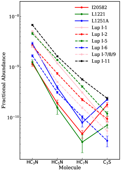
Figure 3: Abundances of detected species.

With the column densities of molecules presented in Table 5, abundances relative to $N$(H₂) (see Table 8) of detected species were obtained, which are given in Table 6. Figure 3 presents the changes of abundances among N-bearing LCCMs HC_2n+1N (n=1-3) and between N-bearing species and C₃S.

For N-bearing species HC_2n+1N (n=1-3), the abundance decreases while n increases. WCCC source Lup I-1 and the five Lupus I starless cores show the highest abundances. Abundances of N-bearing species are lower in the other three outflow sources.

For the molecule C₃S, the abundance in L1251A is the highest among all the detected sources. The abundance of C₃S in I20582 or L1221 is also quite high compared with that of the TMC-1 like cloud Lup I-6. The three outflow sources all have abundances of C₃S larger than that of HC₇N, especially in the case of L1251A in which the abundance of C₃S is even comparable to that of HC₅N.

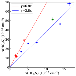
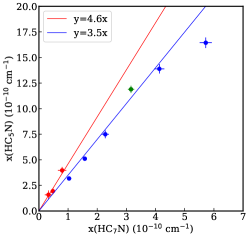
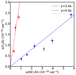
Figure 4: Abundance ratios of different species. Left: x(HC₃N) to x(HC₅N); Middle: x(HC₅N) to x(HC₇N); Right: x(C₃S) to x(HC₇N)). For each panel, the blue line shows the result of linear fitting in bi-logarithm coordinates, and the red line indicates y=$<\frac{y_{i}}{x_{i}}>$x, where $x_{i}$ and $y_{i}$ denote the corresponding abundances for plotted dots. In all panels the blue dots label all the Lup I starless cores, the green dot shows Lup I-1. In this figure the red dotes denote the other three outflows, which were excluded by the correlation between the two parameters of all the Lup I sources.

Table 7 presents the abundance ratios of all the species for all the sources. The ratios of x(HC₃N)/x(HC₅N) for the Lup I starless cores and WCCC source Lup I-1 are all rather close to each other, with an average value of $\sim$3.8. However the ratios of the other three outflow sources are 6.8 on the average and higher than those of the starless cores and the Lup I-1 outflow source. The ratios of x(HC₅N)/x(HC₇N) are 3.6 on the average for all the starless cores and the Lup I-1 outflow source. While the other three outflow sources show an average ratio of 4.6. For the ratio of x(C₃S)/x(HC₇N), the starless cores and the outflow source Lup I-1 have a ratio of 0.4 on the average and the other three outflow sources 3.4, showing the largest difference among the compared ratios. These results indicate that the changes of the CCM emissions with the carbon length in Lup I starless cores and the outflow source Lup I-1 are different from those of the other three outflow sources. The three panels of Figure 4 clearly show that the correlations between each ratio of x(HC₃N)/x(HC₅N), x(HC₅N)/x(HC₇N) and x(C₃S)/x(HC₇N) are different for the starless cores/Lup I-1 outflow source and the other three outflow sources. The difference between the x(C₃S)/x(HC₇N) of the Lup I starless cores/Lup I-1 outflow source and the other three outflow sources is the largest.

4 Discussion

According to their different relative values of abundances of N-bearing CCMs and C₃S, the detected sources can be divided into three groups.

• Group CC includes all the five cold and quiescent dark cores in the Lup I region. Their abundances of N-bearing species decrease with the length of the carbon chains. The ratio x(HC_2n+1N)/x(HC_2n+3N) (n=1-2) is 3.7 on the average. Their ratio of x(C₃S )/x(HC₇N ) is 0.4 on the average.

• Group WC contains Lup I-1 only, which is a known WCCC source. Its ratios of x(HC_2n+1N)/x(HC_2n+3N) (n=1-2) are about the same as those of Group CC. However the ratios of x(C₃S)/x(HC₇N) is 0.3, larger than those of Group CC, which means that C₃S  is more deficient in Lup I-1 than in Group CC sources.

• Group JS consists of I20582, L1221 and L1251A, all with jets and shocks. Their abundances of N-bearing species x(HC_2n+1N) decline faster with the increase of ‘n’ than the other two group sources. Their x(C₃S /x(HC₇N )) ratio is 3.4 on the average, which is in contrast to the same ratios of the sources in the other two groups and it has not been seen previously.

  Below we discuss physical conditions and chemical contents for each group.

4.1 Lupus I starless dust cores

Lupus I is a nearby molecular cloud complex. The distance measured by Lombardi et al. (2008) is 155$\pm$8 pc. For our Lup I cores, except Lup I-1, all are dark and without associated stellar sources within radii of one arcmin except Lup I-5 which contains an object surveyed with Spitzer offset by $\sim$ 0.5 $\arcmin$ from the center (Gaczkowski et al., 2015) . The Herschel 250 µm images of Lup I cores are shown in the bottom panel of Figure A1. The dust temperatures of these cores range from 10.0 to 11.9 K, with an average value of 11.0 K which is similar to that of the cyanopolyyne peak in TMC-1, 10.6 K (Table 8).

The dust cores Lup I-2 and Lup I-5 are located in the gas core C6 where HC₃N J=3-2 and 10-9 were detected (Benedettini et al., 2012). Lup I-6 was identified as a TMC-1 like cloud and is located in the C3 core where HC₃N J=10-9 was detected (Sakai et al., 2010; Benedettini et al., 2012). The gas core C3 also includes the dust core Lup I-7/8/9, which was detected by our TMRT observations too. Lup I-11 is in the gas core C8 where HC₃N J=3-2 and 10-9 were detected (Benedettini et al., 2012). It is also starless with IRAS 15422-3414 located 62 arcsec away.

From Figs. 1 and 2 and Table 3, one can see that CCM emissions of the four dust cores, Lup I-2, Lup I-5, Lup I-7/8/9 and Lup I-11 are all quite strong. Emissions of three (except Lup I-2) of them are even stronger than those of Lup I-6 (Lupus-IA) (Sakai et al., 2010). These results demonstrate that these four starless dust cores detected with LABOCA, Herschel and Planck are all CCM emission cores. The detections of fruitful CCM emissions in Lupus I starless cores as well as in Lup I-1, the second WCCC source (Sakai et al., 2009), indicate that Lupus I is a CCM rich region similar to Taurus.

There is no apparent ongoing star formation in these Lup I cores yet, except Lup I-1. The chemistry of these cores in Lupus I belong to that of a cold and quiescent phase. In this early phase carbon atoms and ions needed to produce carbon-chain molecules arise from photodissociation and photoionization during the diffuse phase of the cloud. In such cloud the C and C⁺ from a more diffuse earlier stage of evolution have not been incorporated into CO yet (Suzuki et al., 1992).

All these starless cores and the outflow source Lup I-1 indicate that the Lup I is a rich CCM and popular carbon-chain–producing region, which may match that of the Taurus molecular complex located at a similar distance from the Sun. This region is located at the edge of the youngest subgroup (Upper-Scorpius) of the Scorpius-Centaurus OB association. It borders the expanding HI shell around the Upper-Scorpius at the north-east side which may represent the source of carbon atoms and ions to form CCMs in the Lup I region (Gaczkowski et al., 2015; Tothill et al., 2009; Suzuki et al., 1992).

The abundance ratios of N-bearing species x(HC_2n+1N)/x(HC_2n+3N) of Lup I starless cores are 3.8 and 3.5 (n=1,2) (Sect 3.4), which is not inconsistent with the values of 2-3 for n=1,2 in dark clouds (Bujarrabal et al., 1981).

About the ratio of x(C₃S)/x(HC₇N), the values of the Lup I starless cores range from 0.3 to 0.5 with an average value of 0.4. It is noteworthy that the x(C₃S)/x(HC₇N) ratio of Lup I-5 is the smallest, which is indicated by the blue point below the blue line in the right panel of Figure 4. The C₃S  emission of this core seems to be influenced by a Spitzer detected c2d source at the 0.5$\arcmin$ from the core center (Gaczkowski et al., 2015).

Regarding the abundance ratio of a source previously detected with the TMRT, Serpens South 1a (Li et al., 2016), the x(HC₃N)/x(HC₅N) and x(HC₅N)/x(HC₇N) ratios are 6.5 and 2.0 respectively, and 4.3 on the average, which is close to those of the Lup I starless cores. The ratio of x(C₃S)/x(HC₇N) is 1.0 which is larger than those of all the Lup I cores. Serpens South 1a is located in the Serpens South Cluster where young stellar objects are embedded. Infall motion was detected with HC₇N  and NH₃. This may be related to the change of the x(C₃S)/x(HC₇N) ratio.

4.2 WCCC source Lup I-1

Lup I-1 is a WCCC source (Sakai et al., 2009) second only to L1527 (Sakai et al., 2008). WCCC sources contain stellar envelope regions with a slightly elevated temperature of $\sim$30 K. In this warmer environment, CH₄ can be evaporated from the dust grain mantles into the surrounding gas, and reacts with C⁺ to produce carbon-chain molecules (Hassel et al., 2008; Sakai et al., 2009; Brown & Charnley, 1991; Millar & Freeman, 1984). Lup I-1 contains a young class 0 stellar object (Yıldız et al., 2015). The bolometric temperature is 52 K, higher than that of L1527 (44 K) (Kristensen et al., 2012). Besides the normal radiation of the protostar, a recent accretion burst likely happened during the last 10² to 10³ yr. This burst might lead to an increase of the stellar luminosity by a factor of 100, which would heat the dust and enhance WCCC emission in this core (Sakai et al., 2008). This was listed as one of the interesting perspectives raised by the recent episodic accretion burst by Jørgensen et al. (2013).

Lup I-1 shows a young molecular outflow driven by a Class 0 object. The outflows traced with CO $J=3-2$ and $6-5$ have an average dynamical time $1.1\times 10^{3}$ yr. The dynamic time given by the lower-J CO line ($J=2-1$) is 2$\times$10³ yr (Tachihara et al., 1996). These time scales are all about one order of magnitude smaller than those of the WCCC source L1527 ($1.1\times 10^{4}$ yr) (Yıldız et al., 2015).

The x(HC₃N)/x(HC₅N) and x(HC₅N)/x(HC₇N) ratios of Lup I-1 are similar to those of the Lup I starless cores. However the x(HC₃N)/x(HC₅N) ratio of the median values of 16 embedded low mass protostars is 8.7, and that of Orion is 13$\pm$6 (Law et al., 2018; Bujarrabal et al., 1981), showing that the changes of emissions from N-bearing species with given length of the carbon chain differ in different star formation regions. In low-mass star formation regions, the cyanopolyynes are usually quite deficient but still closely related (Law et al., 2018). The different x(HC₃N)/x(HC₅N) ratios in starless cores and outflow sources may be caused by the different dominant pathways between HC₃N and HC₅N (Takano et al., 1998; Taniguchi et al., 2016).

The C₃S column density of Lup I-1 is lower than those of HC₃N, HC₅N and HC₇N, and the ratio of x(C₃S)/x(HC₇N) is as small as that of Lup I-5, i. e. the smallest among our targets. It shows that the C₃S abundance in Lup I-1 does not increase as much as in the other three outflow sources (see Sect. 4.4) though HH185 was found within the confines of the outflow region (Tachihara et al., 1996). The reason may be that the CCMs retained from the early core phase keep the abundances of these species at high levels, which might possibly happen during a fast collapse of the cloud’s core like in Lup I-1 (Sakai et al., 2008). Another reason may be that the outflow is very young and there is not enough time for the formation of S-bearing LCCMs from shock induced S⁺.

4.3 Excitation conditions and chemistry in Group JS

4.3.1 Group JS

Three molecular outflow sources, I20582, L1221 and L1251A are included in the Group JS.

In I20582, molecular outflows were detected in the $J=1-0$ lines of CO and ¹³CO (Haikala & Laureijs, 1989; Bally et al., 1995). The outflow age is $\sim 10^{5}$ yr (Tafalla & Myers, 1997). HH 199B1 to HH 199B3 are at or near the CO blue lobe detected with the OVRO interferometer (Arce & Sargent, 2004; Bally et al., 1995). HH 199R1-R5 are located in the north-east and are distributed up to 8′ away from I20582. There is a chain of 2.122 $\mu$m H₂ jet knots through the center and aligned in the south-east to north-west direction (Arce & Sargent, 2004; Bally et al., 1995). The enriched infrared and optical characteristics indicate strong shocks in this source. The observation by Bally et al. (1995) revealed strong S⁺ emission in HH 199B1-B3, B6 and HH 199R2. The peaks of the dense gas detected with CS J=2-1 coincide with the HH 199B1-B3 objects and the CO blue lobe peak, where there is a lack of quiescent gas traced by c-C₃H₂ (Tafalla & Myers, 1997).

L1221 has the highest dust temperature $15.1\pm 0.2$ K among all the LCCM detected sources. CO $J=1-0$ outflows with an age $\sim 5\times 10^{4}$ yr were detected with the 45-m of Nobeyama Radio Observatory (NRO) (Umemoto et al., 1991). It was showing a U-shape distribution resulting from the interaction between the outflow and the surrounding gas (Umemoto et al., 1991). This core therefore appears to be cometary and contains the infrared source IRAS 22266+6845. There is a close binary consisting of two infrared sources located in the east and west of the IRAS source and the eastern one seems to drive the outflow (Lee & Ho, 2005). The source was detected in K^′ band and has a south-eastern extension in the same direction as the eastern lobe of the outflow, showing shocked H₂ emission. HH 363 seen in H$\alpha$ and S⁺ is also associated with the outflow (Alten et al., 1997). Recently, three IRS sources were revealed with Spitzer IRAC/MIPS data and ground based submillimeter emissions. IRS 1 and IRS 2 are Class I objects and IRS 3 is a Class 0 stellar object. IRS 1 contains an arc and IRS 3 a jet. IRS 3 also exhibits 3-6 cm emission which indicates shock ionization due to the interaction between the jet from IRS 3 and the surrounding gas (Young et al., 2009).

Finally, in the outflow source L1251A, a collimated molecular outflow was detected with CO $J=2-1$ line observation by Lee et al. (2010). The dynamical timescale of this outflow is $5.2\times 10^{4}$ yr assuming an inclination angle of 70^∘ (Lee et al., 2010). Spitzer IRAC observations revealed four infrared sources IRS 1-IRS 4. The driving source is IRS 3, a Class 0 object. From this object a collimated long infrared jet originated. Our observed position is 12 arcsec east and 9 arcsec south to IRS 3 (see Figure 6). The detected strong Spitzer IRAC observations revealed a jet with a bipolar structure extending from north to south though IRS 3. The jet may originate from a paraboloidal shock (Lee et al., 2010).

About the N-bearing species in these outflows, the average values of x(HC₃N)/x(HC₅N) and x(HC₅N)/x(HC₇N) are 6.8 and 4.6 respectively, which are both larger than those of the Lup I starless cores and the WCCC source Lup I-1, showing that the abundance of N-bearing species decreases faster with carbon length in these outflows than in starless cores and WCCC sources. The ratio of x(HC₃N)/x(HC₅N) is somewhat lower than the median value (8.7) of 16 low mass protostars detected by Law et al. (2018).

Table 7 shows that in the starless cores, x(C₃S) is two or more times lower than x(HC₇N). The x(C₃S) in the WCCC source Lup I-1 is also three times less than x(HC₇N). While in the other three outflow sources the x(C₃S) are 2-5 times of the x(HC₇N). These results demonstrate that the x(C₃S)/x(HC₇N) values for the three outflows are larger than those of starless cores and the WCCC source almost one order of magnitude higher than their average value.

4.3.2 Chemical mechanism of Group JS sources

The abnormal high abundance of C₃S compared with those of nitrogen-bearing LCCMs in JS sources has not been seen before. Previous studies revealed that the column densities of C₂S have good positive correlation with those of HC₃N and HC₅N in quiescent dark cores (Suzuki et al., 1992). The column densities of C₃S are 3-5 times lower than those of C₂S (Suzuki et al., 1992; Fuente et al., 1990). High C₂S and C₃S abundances were found towards Taurus dark clouds, and there is still a good correlation between column densities of C₂S and HC₅N. In star formation regions, S-bearing CCMs were at best only marginally detected (Suzuki et al., 1992), indicating that the results of our three outflow sources are unusual. WCCC theory was a possible explanation for the large hydrocarbon abundances such as C₄H and C₆H present in L1251A (Cordiner et al., 2011). However, WCCC can not explain the abundances of C₃S in the three outflow sources, since the relative intensities of N-bearing and S-bearing molecules in WCCC sources are close to those in early cold quiescent cores as listed in Table 7.

In the observations of Cordiner et al. (2011) towards L1251A, the C₃S column density is lower than that of HC₇N, which is contrary to our results. Their target point locates at R.A.(2000)=22:30:40.4, Dec.(2000)=75:13:46, while ours (Table 1 and Figure 6) is more than one arcmin closer to IRS3 and the jet (Cordiner et al., 2011; Lee et al., 2010). The associated outflow may heat the surroundings and contribute in inhibiting the depletion of S-molecules (Fuente et al., 2016; Vastel et al., 2018). We speculate that the high abundances of C₃S are relevant to the jets and shocks in the three sources.

These aspects adequately demonstrate that sulfur ions are produced during shock processes developed in these three sources. Shock processes may lead to the reduction of CCMs. However, shocks can fuel the environments with plenty of S⁺ and thus driving the generation of S-bearing CCMs including C₃S. The regions with most abundant S-bearing CCMs do not necessarily completely coincide with the shocked regions since sulfur elements will only enter into S-bearing CCMs through mild chemical reactions. Unlike in cold dark clouds and WCCC sources, shock induced chemistry plays a major role in performances of N- and S-bearing CCMs in these three outflow sources. This is a new chemistry and we name it shocked carbon-chain chemistry (SCCC). The characteristics of our SCCC sources are as following:

1. Their emissions of the N-bearing species are generally weaker than those in early cold and dark cores and WCCC sources. Taking our samples including three SCCC sources and six of the early cold/WCCC sources into account only, the highest column density of HC₃N characterizing the SCCC sources is close to the lowest value of the early cold/WCCC sources.

2. They have relatively strong C₃S emission. Different from the early cold and dark cores and WCCC sources, the column densities of C₃S of SCCC sources exceed those of HC₇N, and this could be used as a criterion to identify SCCC source.

3. The sources are associated with molecular outflows and infrared/optical jets. The dynamic time scales range from 5$\times$10⁴ to 10⁵ yr.

4. Emissions of ionization species, especially S⁺, are enhanced in shocked regions.

4.4 Model test

We modeled the chemistry of WCCC/SCCC sources by treating them as homogeneous, isotropic clouds. In this simulation, a single point chemical network was run under an ordinary differential equation solver DVODE (Brown et al., 1989) with most physical parameters fixed, n(H₂) = 10⁵ cm^-3, A_V = 5 mag, $\sigma$_g = 0.03 $\mu$, and cosmic-ray ionization rate $\gamma$ = $1.2\times 10^{-17}s^{-1}$ (Lee et al., 2004). The metal abundances were adopted as the low-metal abundance case of Graedel et al. (1982), except for that of sulfur. In star-forming regions, the total abundance of sulfur-bearing species is $\sim$ $10^{-8}$ (Li et al., 2016), and this value was adopted instead of the widely used $8\times 10^{-8}$ (Lee et al., 1998). All the elements were initially ionized except for the hydrogen atoms. The network of chemical reactions as well as the binding energies of the species were adopted from the UMIST Database for Astrochemistry (http://www.udfa.net) as described in McElroy et al. (2013). The network consists of 6173 gas phase reactions and 195 reactions on grain surfaces involving 467 atomic and molecular species. The accretion and desorption rates were calculated according to Hasegawa et al. (1992), assuming a sticking coefficient of unity. The temperatures of the gas and dust were assumed to be well coupled. The changes of the fractional abundances of HC_2n+1N (n=1-3) and C₃S with time are shown in the left panel of Figure 5.

The temperature, represented by the dotted green line in the left panel of Figure 5, stays as 15 K till $10^{5}$ yr after the beginning of modeling. Apparently abundances of N- and S-bearing CCMs would increase first and then get depleted significantly before $10^{5}$ yr. During this period, the abundance of C₃S is positively correlated with those of N-bearing CCMs. These characteristics agree with the observations in dark clouds and star-forming sources (Suzuki et al., 1992).

As the temperature increases to 50 K at $1\times 10^{5}$ yr, abundances of N-bearing species increase quickly because of the reactions between the durable nitrogen atoms and the evaporated molecules such as CH₄ and $\mathrm{C_{2}H_{2}}$. Soon after, abundances of N-bearing CCMs drop slowly for the lack of sustained supplements of precursors. The enhancements of N-bearing CCMs with shorter carbon chains, especially HC₃N, are more significant when compared with heavier N-bearing LCCMs. Such a behavior can explain why WCCC sources such as L1527 and our Group JS sources have relatively large x(HC_2n+1N)/x(HC_2n+3N). However, the abundance of C₃S is not enhanced much during this period because sulfur atoms have not been consumed yet, are not as effectively incorporated as nitrogen atoms, and the downward trend of C₃S can not be reversed. These results indicate that, besides hydrocarbons such as C₄H detected in WCCC sources, the N-bearing CCMs will also be largely enhanced in the early phase of WCCC. It can explain the variances between the younger WCCC source Lup I-1 (Sakai et al., 2009) and the older one L1527 (Sakai et al., 2008) whose abundances of N-bearing CCMs are nearly an order of magnitude lower than those of the former one.

Shocks can be the driving sources for a persistent supply of sulfur atoms and ions. The right panel of Figure 5 shows the evolution of the abundances of some important species after a J-shock simulated by the MHD shock code of Flower & Pineau des Forêts (2015). The simulation ran with a magnetic field parameter b = 0.1, a pre-shock density n_H = 10⁵ cm^-3, and shock speed, $v_{s}$ = 5 km s^-1 as described in Hasegawa et al. (1992). The abundances of $N^{+}$, $C^{+}$ and S⁺ would peak at 5$\times$$10^{2}$ yr after the shock, and then decrease because of the piling up of the after-shock fluid and contribute in inhibiting the depletion rates. In realistic cases in molecular clouds, after-shock material can be spread diffusely and bring the shock-induced ions into the environment. A simple order of magnitude estimation can be made to support the idea that the shock can provide enough S⁺ to drive the evolution of sulfur-bearing carbon-chain molecules. Supersonic shocks with a velocity $v_{e}$ = 5 km s^-1 are powerful enough to spur sulfur elements from grain surfaces and to release shocked gas into the environment with S⁺ at abundance $f_{s}=10^{-9}$ (the right panel of Figure 5). For a jet with a mass flux ($S_{s}$) $10^{-7}$ $M_{\sun}$/yr and a velocity ($v_{s}$) 300 km s^-1, the rate of the supplement of sulfur ions to the environment can be estimated as

$$f_{s}(\frac{v_{s}}{v_{e}})^{2}\frac{S_{s}}{M_{env}}\ \sim\ 10^{-20}\ s^{-1}\ per\ H\ atom$$ (3)

in which the envelope mass, $M_{env}$, is taken as 1 solar mass.

After $2\times 10^{5}$ yr, a supplement of S⁺ is applied at a rate of $10^{-20}$ $s^{-1}$ per H atom. The abundance of C₃S rises by one order of magnitude and quickly exceeds that of HC₇N. The artificial supplement of S⁺ is critical for explaining the emission characteristics of S- and N-bearing CCMs in SCCC sources, since WCCC alone can not reproduce the high abundance of C₃S. The abundance of C₃S even exceeds the emission of HC₅N at 2.5$\times$10⁵ yr if the duration of supplementing of S⁺ is not limited. The source L1251A is close to that point with a C₃S column density comparable to that of HC₅N. The time duration between this point and the start of the SCCC process (5$\times$10⁴ yr) is comparable to the dynamical timescale of L1251A (5.2$\times$10⁴ yr; Sect 4.3.2). The column density of C₃S may exceed that of HC₅N in more evolved SCCC sources.

Shocks are more effective in supplying S⁺ than C⁺ and N⁺ (see the right panel of Figure 5). Our sources in the JS group are all associated with HH objects and jets harboring H$\alpha$ lines and S ii features in emission, and shocked regions are reservoirs of $S^{+}$ (Bally et al., 1995; Alten et al., 1997; Lee et al., 2010). The precursors of N-bearing CCMs such as N and C⁺ are more abundant compared with S⁺ (see the left panel of Figure 5) which makes the shock induced enhancements of N-bearing LCCMs relatively ineffective. On the other hand, the pre-consuming of precursors such as CH₄ in the WCCC process would further restrain the enhancements of N-bearing LCCMs. The abundances of N-nearing CCMs are nearly unaffected if supplement rates of C⁺ ($10^{-21}$ s^-1 per H atom) and N⁺ ($10^{-22}$ s^-1 per H atom) are added in the gas-grain model after $2\times 10^{5}$ yr. These characteristics imply that sulfur-containing species are unique tracers of shocks.

5 Summary

Using the new TMRT telescope of the Shanghai Observatory, 11 sources including five outflow sources and six Lupus I starless dust cores were observed measuring HC₃N $J=2-1$, HC₅N $J=6-5$, HC₇N $J=14-13,~{}15-14,~{}16-15$ and C₃S $J=3-2$. Four of the five outflow sources, I20582, L1221, L1251A and Lup I-1 were detected. Among them, I20582 (IRAS20582+7724) and L1221 were newly detected as carbon-chain–producing regions. In the six starless cores of the Lupus I region all the observed transitions were detected except Lup I-3/4. For our detected sources, the excitation temperatures derived from hyperfine component fitting of HC₃N $J=2-1$ are consistent with the dust temperatures derived from Herschel data. Column densities are calculated. Abundances were derived and analyzed for different kinds of species and sources. The main results are as follows:

1. Emission of C₃S $J=3-2$ in the three outflow sources I20582, L1221 and L1521A was found stronger than their HC₇N emissions, which can not be explained by chemistry of early cold and dark cores and warm carbon-chain chemistry (WCCC) sources. Shock carbon-chain chemistry (SCCC) is suggested. In SCCC sources, shocks fuel the environments with abundant S⁺ and thus drive the generation of S-bearing CCMs including C₃S.

2. In the other outflow source Lup I-1 all the observed lines are strong. However, emission of the C₃S is still weaker than those of the detected N-bearing species in this source, similar to the cases in the starless cores in the Lupus region. In young SCCC sources such as L1251A, WCCC can still play a role in local regions.

3. Emissions of N- and S-bearing CCMs of starless cores in Lupus I are pretty strong, and those of Lup I-11, Lup I-5 and Lup I-7/8/9 are even stronger than those of the TMC-1 like cloud Lup I-6 (Lupus-1A). The results of these cores and Lup I-1 show that Lupus I is a carbon-chain molecule( CCM) rich complex similar to the Taurus complex.

4. Our gas-grain chemical model shows that SCCC is necessary to explain the observations toward the three above mentioned outflow sources since the WCCC can enhance the abundances of N-bearing CCMs while it does not strongly influence the S-bearing CCMs. Shock feedback by protostars can provide enough S⁺ to drive SCCC. Our results demonstrate that the chemistry of S- and N-bearing species can be different in molecular outflow/jet sources. More observations are needed to further explore SCCC.

Figure 1: HC₃N Spectra.

Figure 2: Spectra of HC₅N, HC₇N and C₃S.

Figure 2: Continued.

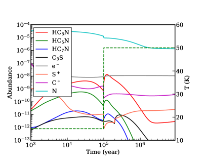
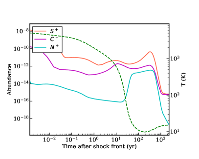
Figure 5: Left: Abundances of carbon-chain molecules from our single point gas-grain chemical model for cold/warm gas; Right: Abundances of some elementary ions after the passage of a shock (Flower & Pineau des Forêts, 2012, 2015). The dotted green line represents gas temperature.

Table 1: Sources

Name	Ra(J2000)	Dec(J2000)	D(pc)	Notes	Reference	Observation date
L1660	07:20:06.75	-24:02:20.9	1000	Molecular outflow	a	2016.03.24
IRAS 20582+7724	20:57:10.6	+77:35:46	200	Molecular outflow, L1228	b	2016.01.25/26,2017,11,9
L1221	22:28:02.7	+69:01:13	200	Molecular outflow	c	2016.01.26,2017,11,9
L1251A	22:30:35.0	+75:14:00	330	Molecular outflow	d	2015.12.16, 2016.01.25
Lup I-1	15:43:01.68	-34:09:08.9	155	Molecular outflow,WCCC	e	2016.03.21
Lup I-2	15:44:59.8	-34:17:09	155	In Lup1 C6	f	2016.01.25
Lup I-3/4	15:45:14.8	-34:17:02.7	155	In Lup1 C7	f	2016.03.21
Lup I-5	15:45:03.80	-34:17:57.3	155	In Lup1 C6	f	2016.03.21
Lup I-6	15:42:52.4	-34:07:54	155	Lupus-1A, in Lup1 C3	g	2016.01.25
Lup I-7/8/9	15:42:44.06	-34:08:30.4	155	In Lup1 C3	f	2016.03.24
Lup I-11	15:45:25.10	-34:24:01.8	155	In Lup1 C8	f	2016.03.24

^aLee & Ho (2005); Davis et al. (1997); Wu et al. (2004) and the references therein; ^bDevine et al. (2009); ^cUmemoto et al. (1991); ^dCordiner et al. (2011); ^eGaczkowski et al. (2015); Benedettini et al. (2012); Sakai et al. (2009); Lombardi et al. (2008); ^fGaczkowski et al. (2015); Benedettini et al. (2012); Lombardi et al. (2008); ^gGaczkowski et al. (2015); Benedettini et al. (2012); Sakai et al. (2010); Lombardi et al. (2008)

Table 2: Observed line and telescope parameters

Molecular	Transition	freq.(MHz)	$Log_{10}(A_{ij}\ s^{-1})$	$E_{up}(K)$	HPBWs (”)
HC3N	J=2-1 F=1-1	18198.3745	-7.26550	1.30990	52
	J=2-1 F=3-2	18196.3104	-6.88533	1.30995	52
	J=2-1 F=2-1	18196.2169	-7.01030	1.30980	52
	J=2-1 F=1-0	18195.1364	-7.14068	1.31003	52
	J=2-1 F=2-2	18194.9195	-7.48753	1.30988	52
HC5N	J=6-5 F=7-6	15975.9831	-6.86356	2.68359	60
	J=6-5 F=6-5	15975.9663	-6.87581	2.68345	60
	J=6-5 F=5-4	15975.9336	-6.87816	2.68359	60
HC7N	J=16-15	18047.9697	-6.11305	7.36235	53
	J=15-14	16919.9791	-6.19805	6.49617	56
	J=14-13	15791.9870	-6.28888	5.68424	60
C3S	J=3-2	17342.2564	-6.44743	1.66464	55

Table 3: Observed Parameters

Lines	Transition	I20582	L1221	L1251A	LupusI-1	LupusI-2	LupusI-5	LupusI-6	LupusI-7/8/9	LupusI-11
		Part I  Vlsr ($\mathrm{km~{}s^{-1}}$)
HC3N	J=2-1 F=1-1	-8.1(1)	-4.53(4)	-3.92(3)	5.11(2)	4.88(3)	4.97(3)	5.13(2)	5.13(2)	4.38(2)
	J=2-1 F=3-2	-8.04(3)	-4.49(3)	-3.96(2)	5.10(2)	4.87(2)	4.95(2)	5.12(2)	5.14(2)	4.37(2)
	J=2-1 F=2-1	-8.06(4)	-4.51(4)	-3.95(2)	5.10(2)	4.86(2)	4.94(2)	5.12(2)	5.14(2)	4.37(2)
	J=2-1 F=1-0	-8.01(3)	-4.47(4)	-3.97(3)	5.09(2)	4.86(3)	4.94(3)	5.11(2)	5.14(2)	4.37(2)
	J=2-1 F=2-2	-8.12(6)	-4.46(5)	-3.96(4)	5.09(2)	4.84(3)	4.99(3)	5.14(2)	5.13(2)	4.37(2)
HC5N	J=6-5 F=7-6			-3.79(3)	5.08(2)	4.94(2)	5.09(2)	5.11(2)	5.14(2)	4.39(2)
	J=6-5 F=6-5	-8.00(4)	-4.59(5)		5.08(2)			5.11(2)	5.14(2)	4.39(2)
	J=6-5 F=5-4			-3.97(3)	5.09(4)	4.89(2)	4.96(2)	5.11(3)	5.14(2)	4.38(2)
HC7N	J=16-15	-7.95(7)		-4.00(3)	5.10(2)	4.87(3)	4.96(3)	5.11(2)	5.14(2)	4.39(2)
	J=15-14		-4.49(9)	-3.96(4)	5.09(2)	4.83(3)	4.95(2)	5.10(3)	5.14(2)	4.39(2)
	J=14-13	-7.73(8)		-4.09(6)	5.08(2)	4.82(3)	4.94(2)	5.12(2)	5.12(2)	4.37(2)
C3S	J=3-2	-8.07(5)	-4.55(5)	-3.98(2)	5.12(3)	4.71(4)	4.94(3)	5.10(4)	5.14(3)	4.37(2)
		Part II  $T_{\mathrm{MB}}$ (K)
HC3N	J=2-1 F=1-1	0.05(2)	0.09(2)	0.37(8)	1.5(2)	0.38(8)	0.7(2)	0.59(9)	1.0(1)	0.88(9)
	J=2-1 F=3-2	0.28(2)	0.30(2)	1.57(8)	5.1(2)	1.71(9)	2.9(2)	2.04(9)	4.1(1)	3.50(9)
	J=2-1 F=2-1	0.15(2)	0.21(2)	0.83(8)	3.2(2)	1.08(9)	1.7(2)	1.39(9)	2.6(1)	2.30(9)
	J=2-1 F=1-0	0.08(2)	0.13(2)	0.36(8)	1.6(2)	0.48(9)	0.9(2)	0.82(9)	1.3(1)	1.17(9)
	J=2-1 F=2-2	0.06(2)	0.08(2)	0.22(8)	1.1(2)	0.39(9)	0.55(2)	0.63(9)	1.2(1)	0.97(9)
HC5N	J=6-5 F=7-6			0.20(3)	1.28(5)	0.53(4)	1.01(5)	0.62(5)	0.93(5)	1.00(5)
	J=6-5 F=6-5	0.061(7)	0.057(8)		1.08(5)			0.47(5)	0.79(5)	0.90(5)
	J=6-5 F=5-4			0.14(3)	0.92(5)	0.34(4)	0.61(6)	0.42(5)	0.70(5)	0.81(5)
HC7N	J=16-15	0.037(8)		0.08(4)	0.76(7)	0.28(5)	0.54(7)	0.40(5)	0.55(5)	0.65(5)
	J=15-14		0.026(8)	0.10(4)	8.3(7)	0.26(5)	0.54(7)	0.30(5)	0.53(5)	0.63(6)
	J=14-13	0.030(8)		0.06(4)	0.75(7)	0.31(5)	0.65(7)	0.38(5)	0.44(4)	0.72(6)
C3S	J=3-2	0.049(8)	0.036(8)	0.26(4)	0.22(6)	0.11(4)	0.25(6)	0.10(5)	0.13(4)	0.32(4)
		Part III  FWHM (km s-1)
HC3N	J=2-1 F=1-1	1.0(2)	0.4(1)	0.36(5)	0.19(2)	0.45(4)	0.33(4)	0.22(3)	0.18(3)	0.22(3)
	J=2-1 F=3-2	0.85(4)	0.74(4)	0.34(2)	0.25(2)	0.42(2)	0.42(2)	0.26(2)	0.21(2)	0.23(4)
	J=2-1 F=2-1	0.90(7)	0.80(6)	0.36(3)	0.25(2)	0.39(3)	0.41(3)	0.24(3)	0.20(2)	0.22(2)
	J=2-1 F=1-0	1.0(1)	0.54(8)	0.35(3)	0.23(3)	0.44(4)	0.41(3)	0.20(3)	0.18(3)	0.21(2)
	J=2-1 F=2-2	0.6(1)	0.5(1)	0.40(5)	0.24(3)	0.40(4)	0.50(5)	0.18(3)	0.17(3)	0.22(3)
HC5N	J=6-5 F=7-6				0.21(2)	0.67(3)	0.59(2)	0.19(3)	0.18(2)	0.23(2)
	J=6-5 F=6-5	1.31(8)	0.8(1)	0.56(3)	0.27(3)			0.19(3)	0.16(2)	0.18(2)
	J=6-5 F=5-4			0.39(4)	0.23(2)	0.37(3)	0.39(3)	0.18(2)	0.16(2)	0.18(2)
HC7N	J=16-15	0.9(1)		0.35(7)	0.29(2)	0.43(4)	0.42(4)	0.18(2)	0.19(2)	0.25(2)
	J=15-14		0.64(3)	0.31(5)	0.26(2)	0.46(4)	0.42(3)	0.25(3)	0.20(2)	0.27(2)
	J=14-13	0.6(2)		0.6(1)	0.31(2)	0.49(3)	0.41(3)	0.22(3)	0.25(2)	0.26(2)
C3S	J=3-2	1.4(2)	0.8(1)	0.32(3)	0.24(3)	0.54(2)	0.30(4)	0.3(1)	0.35(5)	0.24(3)
		Part IV  Area (K km s-1)
HC3N	J=2-1 F=1-1	0.041(8)	0.033(6)	0.14(2)	0.30(2)	0.18(2)	0.25(2)	0.14(1)	0.19(1)	0.20(1)
	J=2-1 F=3-2	0.26(1)	0.23(1)	0.57(2)	1.38(5)	0.77(3)	1.27(4)	0.55(2)	0.90(3)	0.85(3)
	J=2-1 F=2-1	0.13(1)	0.14(1)	0.32(1)	0.84(3)	0.45(2)	0.78(3)	0.36(2)	0.55(2)	0.54(2)
	J=2-1 F=1-0	0.066(7)	0.053(7)	0.13(1)	0.40(2)	0.23(2)	0.41(3)	0.18(1)	0.25(1)	0.27(1)
	J=2-1 F=2-2	0.031(6)	0.035(7)	0.10(1)	0.30(2)	0.17(1)	0.30(3)	0.12(1)	0.21(1)	0.23(1)
HC5N	J=6-5 F=7-6			0.12(1)	0.28(1)	0.38(1)	0.64(2)	0.12(1)	0.18(1)	0.24(1)
	J=6-5 F=6-5	0.077(4)	0.058(5)		0.31(1)			0.096(6)	0.013(6)	0.174(7)
	J=6-5 F=5-4			0.041(4)	0.23(1)	0.13(1)	0.25(1)	0.080(5)	0.118(6)	0.158(6)
HC7N	J=16-15	0.026(4)		0.031(6)	0.24(1)	0.13(1)	0.24(1)	0.077(6)	0.109(6)	0.168(6)
	J=15-14		0.013(3)	0.031(5)	0.23(1)	0.126(8)	0.24(1)	0.078(7)	0.110(6)	0.18(1)
	J=14-13	0.014(3)		0.038(7)	0.25(1)	0.16(1)	0.28(1)	0.089(6)	0.116(6)	0.199(9)
C3S	J=3-2	0.069(7)	0.024(3)	0.088(6)	0.054(7)	0.064(7)	0.079(8)	0.033(8)	0.046(6)	0.083(6)

Table 4: HC₃N HFS fitting

Sources	$\tau$(HC3N)	Tex(HC3N)	Td
		K	K
I20582	$<$0.1	–	13.5(0.3)
L1221	0.28(0.19)	14.02(5.11)	15.1(0.2)
L1251A	$<$0.1	–	12.4(0.2)
LupusI-1	0.84(0.08)	15.79(1.69)	13.9(0.1)
LupusI-2	0.55(0.11)	9.52(1.32)	11.5(0.2)
LupusI-5	0.72(0.13)	11.93(1.71)	11.2(0.1)
LupusI-6	1.43(0.13)	7.03(0.52)	10.0(0.2)
LupusI-7/8/9	0.85(0.08)	14.50(1.33)	10.2(0.1)
LupusI-11	1.07(0.08)	11.39(0.77)	11.9(0.8)

Table 5: Column densities derived from each line component (in units of 10¹² cm^-2)

Lines	Transition	I20582	L1221	L1251A	LupusI-1	LupusI-2	LupusI-5	LupusI-6	LupusI-7/8/9	LupusI-11
		Part I  Column density derived from each line component ($10^{12}$ cm-2)
HC3N	J=2-1 F=1-1	21(4)	20(3)	69(6)	157(8)	83(6)	112(11)	57(4)	80(4)	98(5)
	J=2-1 F=3-2	23.8(0.7)	28(1)	49.4(1.0)	131(1)	63(1)	104(2)	42.1(0.8)	69.7(0.8)	72.1(0.9)
	J=2-1 F=2-1	22(1)	30(1)	52(1)	148(3)	69(2)	118(3)	50(1)	79(1)	85(1)
	J=2-1 F=1-0	25(2)	25(3)	49(4)	157(7)	79(5)	139(8)	56(3)	80(3)	95(3)
	J=2-1 F=2-2	16(3)	22(4)	46(5)	156(10)	78(6)	135(12)	52(3)	89(4)	107(4)
HC5N	J=6-5 F=7-6			7.8(0.6)	35(1)	24(1)	40(1)	12.7(0.5)	19.1(0.5)	27.8(0.8)
	J=6-5 F=6-5	3.6(0.6)	3.2(0.8)		46(1)			11.9(0.6)	16.4(0.6)	23.6(0.8)
	J=6-5 F=5-4			6.7(0.7)	40(1)	20(1)	39(1)	11.8(0.7)	17.5(0.7)	25.4(0.8)
HC7N	J=16-15	1.1(0.2)		1.3(0.2)	10.0(0.3)	5.2(0.3)	9.8(0.4)	3.1(0.2)	4.4(0.2)	6.9(0.2)
	J=15-14		0.7(0.2)	1.4(0.2)	10.2(0.4)	5.4(0.3)	10.2(0.4)	3.3(0.3)	4.6(0.2)	7.8(0.3)
	J=14-13	0.7(0.1)		1.8(0.3)	12.2(0.4)	7.6(0.4)	13.0(0.5)	4.0(0.3)	5.2(0.2)	9.3(0.3)
C3S	J=3-2	3.5(0.4)	1.4(0.2)	4.2(0.2)	2.8(0.4)	2.9(0.3)	3.5(0.4)	1.4(0.3)	2.0(0.3)	3.9(0.2)
		Part II  Column density for each specie ($10^{12}$ cm-2)
HC3N		21(2)	25(2)	53(3)	150(6)	74(4)	121(7)	52(2)	79(3)	91(3)
HC5N		3.6(0.6)	3.2(0.8)	7.3(0.6)	40(1)	22(1)	39(1)	12.1(0.6)	17.7(0.6)	25.6(0.8)
HC7N		0.9(0.2)	0.7(0.1)	1.5(0.3)	10.8(0.4)	6.1(0.3)	11.0(0.4)	3.5(0.2)	4.7(0.2)	8.0(0.3)
C3S		3.5(0.4)	1.4(0.2)	4.2(0.2)	2.8(0.4)	2.9(0.3)	3.5(0.4)	1.4(0.3)	2.0(0.3)	3.9(0.2)

Table 6: Abundances (in unit $10^{-10}$)

Sources	HC3N	HC5N	HC7N	C3S
I20582	10(1)	1.7(0.3)	0.42(0.07)	1.7(0.2)
L1221	16(1)	2.2(0.4)	0.5(0.1)	1.01(0.08)
L1251A	26(1)	3.6(0.3)	0.7(0.1)	2.1(0.1)
LupusI-1	40(1)	11.0(0.3)	2.92(0.10)	0.76(0.10)
LupusI-2	25(1)	7.7(0.4)	2.1(0.1)	1.0(0.1)
LupusI-5	43(2)	14.2(0.5)	3.9(0.2)	1.3(0.1)
LupusI-6	13(1)	3.1(0.2)	0.89(0.06)	0.36(0.09)
LupusI-7/8/9	23(1)	5.0(0.2)	1.36(0.06)	0.56(0.07)
LupusI-11	61(2)	17.1(0.5)	5.3(0.2)	2.6(0.2)

Table 7: Abundance ratio

Sources	x(HC3N)		x(HC5N)		x(C3S)
	/x(HC5N)	Average	/x(HC7N)	Average	/x(HC7N)	Average
I20582	5.8		4.0		5.0
L1221	7.3		5.0		2.0
L1251A	7.3	6.8	4.9	4.6	3.3	3.4
LupusI-1	3,8	3.8	3.7	3.7	0.3	0.3
LupusI-2	3.3		3.6		0.5
LupusI-5	3.1		3.5		0.3
LupusI-6	4.3		3.5		0.4
LupusI-7/8/9	4.5		3.8		0.4
LupusI-11	3.6	3.8	3.2	3.5	0.5	0.4

Appendix A Dust Temperatures and Column Densities

All the sources observed except L1660 have Herschel data at 70, 160, 250, 350, and 500 $\mu$m in the Herschel Science Archive, where we extracted Level 2 or Level 2.5 images. These data, which are from the Gould Belt Survey and a few other Herschel key programs and open time programs, have resolutions of 8.$\!\!\arcsec$4, 13.$\!\!\arcsec$5, 18.$\!\!\arcsec$1, 24.$\!\!\arcsec$9 and 36.$\!\!\arcsec$4 at 70, 160, 250, 350, and 500 $\mu$m respectively^,, and the corresponding pixel sizes are 3.$\!\!\arcsec$2, 3.$\!\!\arcsec$2, 6.$\!\!\arcsec$0, 10.$\!\!\arcsec$0 and 14.$\!\!\arcsec$0. On the basis of these multi-bands far-IR data, we obtained dust temperatures and column densities.

A.1 Background Removal

Background/foreground emission was removed using the CUPID-findback algorithm of the Starlink suite (Currie et al., 2014). The algorithm constructs the background iteratively from the original image. At first, a filtered form of the input data is produced by replacing every input pixel by the minimum of the input values within a rectangular box centered on the pixel. This filtered data is then filtered again, using a filter that replaces every pixel value by the maximum value in a box centered on the pixel. Then each pixel in this filtered data is replaced by the mean value in a box centered on the pixel. The same box size is used for the first three steps. The final background estimate is obtained via some corrections and iterations by comparisons with the initial input data. More details about the algorithm can be found on the online document of findback. As a key parameter, the box has been assigned to be the source size at 250 µm which was measured based on the area with emission higher than 50% of the peak intensity for each target.

A.2 Flux Measurements

For each source, we firstly determined the source size based on the emission at 250 µm (Figure 6) via fitting an ellipse to the region with emission higher than 50% of the peak intensity around the target. Then fluxes at other bands were obtained by integrating the emission encompassed by the ellipse if the ellipse was larger than the beam. Otherwise fluxes referring to the beam centered at the source have been used. The source size at 250 µm and fluxes at Herschel bands are given in 2ed-7th column of Table 8.

A.3 Spectral Energy Distribution Fitting

The fluxes at Herschel bands have been modeled using single temperature gray-bodies,

$$S_{\nu}=B_{\nu}(T)(1-e^{-\tau_{\nu}})\Omega$$ (4)

where the Planck function $B_{\nu}(T)$ is modified by the optical depth

$$\tau_{\nu}=\mu_{\mathrm{H_{2}}}m_{\mathrm{H}}\kappa_{\nu}N_{\mathrm{H_{2}}}/R_{\mathrm{gd}}.$$ (5)

Here, $\mu_{\mathrm{H_{2}}}=2.8$ is the mean molecular weight adopted from Kauffmann et al. (2008), $m_{\mathrm{H}}$ is the mass of a hydrogen atom, $N_{\mathrm{H_{2}}}$ is the column density, $R_{\mathrm{gd}}=100$ is the gas to dust ratio. The dust opacity $\kappa_{\nu}$ can be expressed as a power law of frequency,

$$\kappa_{\nu}=5.9\left(\frac{\nu}{850~{}\mathrm{GHz}}\right)^{\beta}~{}\mathrm{cm^{2}g^{-1}}.$$ (6)

with $\kappa_{\nu}(\mathrm{850~{}GHz})=5.9~{}\mathrm{cm^{2}g^{-1}}$ adopted from Ossenkopf & Henning (1994). The $\Omega$ in Equation 4 is the solid angle of the target. The free parameters are the dust temperature, dust emissivity index $\beta$ and column density.

The fluxes at 70 $\mu$m were excluded from the SED fitting because emission at this wavelength may arise from a warmer dust component and a large fraction of the 70 $\mu$m emission originates from very small grains, where the assumption of a single equilibrium temperature is not valid.

The fitting was performed with the Levenberg-Marquardt algorithm provided in the python package lmfit (Newville et al., 2016). Fitted SED curves were shown in Figure 7. The resulting dust temperatures and column densities are listed in columns 8 and 9 of Table 8.

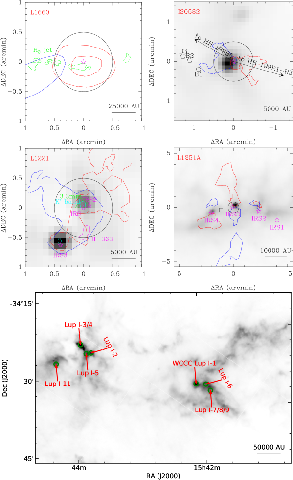
Figure 6: Upper 4 panels show materials covered within a single beam (black circle) for outflow sources L1660 (Davis et al., 1997; Schwartz et al., 1988), I20582 (Arce & Sargent, 2004), L1221 (Alten et al., 1997; Lee & Ho, 2005; Young et al., 2009) and L1251A (Lee et al., 2010). Blue and red lobes of CO outflows are roughly sketched by blue and red solid lines. The black square in the panel of L1251A denotes the point observed by Cordiner et al. (2011). Bottom panel shows the locations of the observed Lupus I cores and the beams (green circles). Background are Herschel 250 $\mu$m maps (André et al., 2010; Rygl et al., 2013).

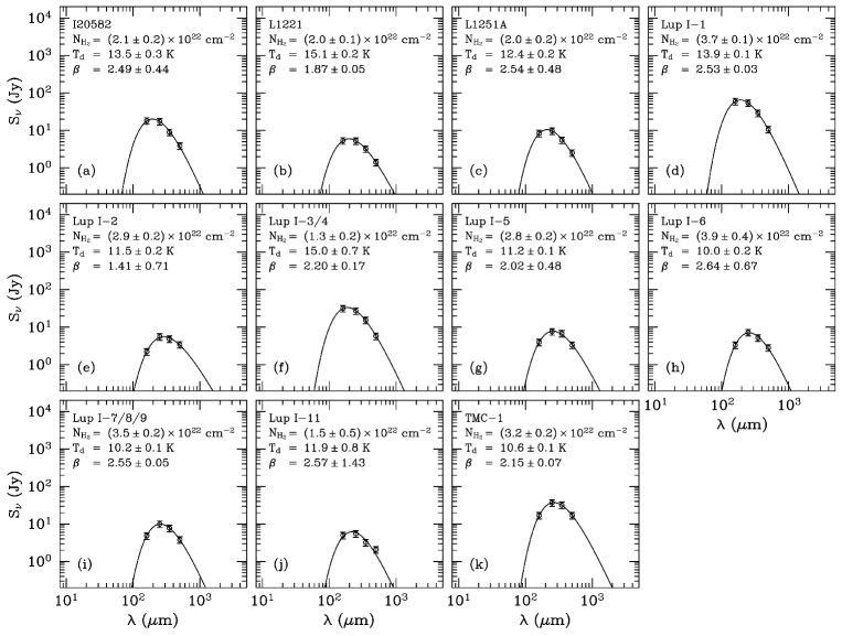
Figure 7: SED of the observed sources. For comparisions the SED of TMC-1 is also presented. The filled circles are the data points used for the SED fitting. The error bar of each point is plotted.

Table 8: Dust Parameters

Source	S70	S160	S250	S350	S500	Size250	Tdust	N${}_{\mathrm{H_{2}}}$
	Jy	Jy	Jy	Jy	Jy	arcsec	K	$10^{22}$ cm-2
IRAS20582+7724	9.04	18.14	17.28	8.94	3.89	43.16	13.5(0.3)	2.1(0.2)
L1221	6.22	5.34	5.28	3.23	1.40	21.91	15.1(0.2)	2.0(0.1)
L1251A	1.75	8.35	9.77	5.50	2.53	40.67	12.4(0.2)	2.0(0.2)
Lupus1-1	21.49	59.44	54.10	29.07	10.67	55.00	13.9(0.1)	3.7(0.1)
Lupus1-2	0.19	2.24	5.61	4.86	3.44	36.00	11.5(0.2)	2.9(0.2)
Lupus1-3/4	8.86	31.73	27.13	15.37	5.83	57.96	15.0(0.7)	1.3(0.2)
Lupus1-5	0.25	4.00	7.67	6.79	3.32	42.69	11.2(0.1)	2.8(0.2)
Lupus1-6	0.04	3.34	7.26	5.22	2.87	43.00	10.0(0.2)	3.9(0.4)
Lupus1-7/8/9	0.00	4.86	10.00	7.79	3.80	50.42	10.2(0.1)	3.5(0.2)
Lupus1-11	0.32	3.31	5.50	3.21	2.08	39.20	11.9(0.8)	1.5(0.5)
TMC-1	0.14	16.95	36.78	31.92	16.96	100.00	10.6(0.1)	3.2(0.2)

References

- Alten et al. (1997) Alten V. P., Bally J., Devine D., Miller G. J., 1997, in Reipurth B., Bertout C., eds, IAU Symposium Vol. 182, Herbig-Haro Flows and the Birth of Stars. p. 51
- André et al. (2010) André P., et al., 2010, A&A, 518, L102
- Arce & Sargent (2004) Arce H. G., Sargent A. I., 2004, ApJ, 612, 342
- Avery et al. (1976) Avery L. W., Broten N. W., MacLeod J. M., Oka T., Kroto H. W., 1976, ApJ, 205, L173
- Bally et al. (1995) Bally J., Devine D., Fesen R. A., Lane A. P., 1995, ApJ, 454, 345
- Bell et al. (1997) Bell M. B., Feldman P. A., Travers M. J., McCarthy M. C., Gottlieb C. A., Thaddeus P., 1997, ApJ, 483, L61
- Benedettini et al. (2012) Benedettini M., Pezzuto S., Burton M. G., Viti S., Molinari S., Caselli P., Testi L., 2012, MNRAS, 419, 238
- Bernes (1977) Bernes C., 1977, A&AS, 29, 65
- Brown & Charnley (1991) Brown P. D., Charnley S. B., 1991, MNRAS, 249, 69
- Brown et al. (1989) Brown P., Byrne G., Hindmarsh A., 1989, SIAM Journal on Scientific and Statistical Computing, 10, 1038
- Bujarrabal et al. (1981) Bujarrabal V., Guelin M., Morris M., Thaddeus P., 1981, A&A, 99, 239
- Bussa & VEGAS Development Team (2012) Bussa S., VEGAS Development Team 2012, in American Astronomical Society Meeting Abstracts #219. p. 446.10
- Cordiner et al. (2011) Cordiner M. A., Charnley S. B., Buckle J. V., Walsh C., Millar T. J., 2011, ApJ, 730, L18
- Currie et al. (2014) Currie M. J., Berry D. S., Jenness T., Gibb A. G., Bell G. S., Draper P. W., 2014, in Manset N., Forshay P., eds, Astronomical Society of the Pacific Conference Series Vol. 485, Astronomical Data Analysis Software and Systems XXIII. p. 391
- Davis et al. (1997) Davis C. J., Ray T. P., Eisloeffel J., Corcoran D., 1997, A&A, 324, 263
- Devine et al. (2009) Devine D., Bally J., Chiriboga D., Smart K., 2009, AJ, 137, 3993
- Dickens et al. (2001) Dickens J. E., Langer W. D., Velusamy T., 2001, ApJ, 558, 693
- Flower & Pineau des Forêts (2012) Flower D. R., Pineau des Forêts G., 2012, MNRAS, 421, 2786
- Flower & Pineau des Forêts (2015) Flower D. R., Pineau des Forêts G., 2015, A&A, 578, A63
- Friesen et al. (2013) Friesen R. K., Medeiros L., Schnee S., Bourke T. L., Francesco J. D., Gutermuth R., Myers P. C., 2013, MNRAS, 436, 1513
- Fuente et al. (1990) Fuente A., Cernicharo J., Barcia A., Gomez-Gonzalez J., 1990, A&A, 231, 151
- Fuente et al. (2016) Fuente A., et al., 2016, A&A, 593, A94
- Gaczkowski et al. (2015) Gaczkowski B., et al., 2015, A&A, 584, A36
- Garden et al. (1991) Garden R. P., Hayashi M., Hasegawa T., Gatley I., Kaifu N., 1991, ApJ, 374, 540
- Graedel et al. (1982) Graedel T. E., Langer W. D., Frerking M. A., 1982, ApJS, 48, 321
- Gratier et al. (2013) Gratier P., Pety J., Guzmán V., Gerin M., Goicoechea J. R., Roueff E., Faure A., 2013, A&A, 557, A101
- Guilloteau & Lucas (2000) Guilloteau S., Lucas R., 2000, in Mangum J. G., Radford S. J. E., eds, Astronomical Society of the Pacific Conference Series Vol. 217, Imaging at Radio through Submillimeter Wavelengths. p. 299
- Haikala & Laureijs (1989) Haikala L. K., Laureijs R. J., 1989, A&A, 223, 287
- Hasegawa et al. (1992) Hasegawa T. I., Herbst E., Leung C. M., 1992, ApJS, 82, 167
- Hassel et al. (2008) Hassel G. E., Herbst E., Garrod R. T., 2008, ApJ, 681, 1385
- Hirota & Yamamoto (2006) Hirota T., Yamamoto S., 2006, ApJ, 646, 258
- Hirota et al. (2009) Hirota T., Ohishi M., Yamamoto S., 2009, ApJ, 699, 585
- Inostroza et al. (2011) Inostroza N., Huang X., Lee T. J., 2011, J. Chem. Phys., 135, 244310
- Irvine et al. (1988) Irvine W. M., Ziurys L. M., Avery L. W., Matthews H. E., Friberg P., 1988, Astrophysical Letters and Communications, 26, 167
- Jørgensen et al. (2013) Jørgensen J. K., et al., 2013, ApJ, 779, L22
- Kaifu et al. (2004) Kaifu N., et al., 2004, PASJ, 56, 69
- Kauffmann et al. (2008) Kauffmann J., Bertoldi F., Bourke T. L., Evans II N. J., Lee C. W., 2008, A&A, 487, 993
- Kristensen et al. (2012) Kristensen L. E., et al., 2012, A&A, 542, A8
- Langer et al. (1980) Langer W. D., Schloerb F. P., Snell R. L., Young J. S., 1980, in Bulletin of the American Astronomical Society. p. 485
- Law et al. (2018) Law C. J., Öberg K. I., Bergner J. B., Graninger D., 2018, ApJ, 863, 88
- Lee & Ho (2005) Lee C.-F., Ho P. T. P., 2005, ApJ, 632, 964
- Lee et al. (1998) Lee H.-H., Roueff E., Pineau des Forets G., Shalabiea O. M., Terzieva R., Herbst E., 1998, A&A, 334, 1047
- Lee et al. (2004) Lee J.-E., Bergin E. A., Evans II N. J., 2004, ApJ, 617, 360
- Lee et al. (2010) Lee J.-E., et al., 2010, ApJ, 709, L74
- Li et al. (2016) Li J., et al., 2016, ApJ, 824, 136
- Liszt et al. (2012) Liszt H., Sonnentrucker P., Cordiner M., Gerin M., 2012, ApJ, 753, L28
- Loison et al. (2014) Loison J.-C., Wakelam V., Hickson K. M., Bergeat A., Mereau R., 2014, MNRAS, 437, 930
- Lombardi et al. (2008) Lombardi M., Lada C. J., Alves J., 2008, A&A, 480, 785
- Lucas & Liszt (2000) Lucas R., Liszt H. S., 2000, A&A, 358, 1069
- Magakian (2003) Magakian T. Y., 2003, A&A, 399, 141
- Mangum & Shirley (2015) Mangum J. G., Shirley Y. L., 2015, PASP, 127, 266
- Matthews et al. (1984) Matthews H. E., Irvine W. M., Friberg P., Brown R. D., Godfrey P. D., 1984, Nature, 310, 125
- McElroy et al. (2013) McElroy D., Walsh C., Markwick A. J., Cordiner M. A., Smith K., Millar T. J., 2013, A&A, 550, A36
- McGuire et al. (2017) McGuire B. A., Burkhardt A. M., Shingledecker C. N., Kalenskii S. V., Herbst E., Remijan A. J., McCarthy M. C., 2017, ApJ, 843, L28
- Millar & Freeman (1984) Millar T. J., Freeman A., 1984, MNRAS, 207, 405
- Mitchell & Huntress (1979) Mitchell G. F., Huntress Jr. W. T., 1979, Nature, 278, 722
- Newville et al. (2016) Newville M., Stensitzki T., Allen D. B., Rawlik M., Ingargiola A., Nelson A., 2016, Lmfit: Non-Linear Least-Square Minimization and Curve-Fitting for Python, Astrophysics Source Code Library (ascl:1606.014), doi:10.5281/zenodo.49428
- Ohashi et al. (1999) Ohashi N., Lee S. W., Wilner D. J., Hayashi M., 1999, ApJ, 518, L41
- Ossenkopf & Henning (1994) Ossenkopf V., Henning T., 1994, A&A, 291, 943
- Pety et al. (2005) Pety J., Teyssier D., Fossé D., Gerin M., Roueff E., Abergel A., Habart E., Cernicharo J., 2005, A&A, 435, 885
- Rygl et al. (2013) Rygl K. L. J., et al., 2013, A&A, 549, L1
- Sakai et al. (2008) Sakai N., Sakai T., Hirota T., Yamamoto S., 2008, ApJ, 672, 371
- Sakai et al. (2009) Sakai N., Sakai T., Hirota T., Burton M., Yamamoto S., 2009, ApJ, 697, 769
- Sakai et al. (2010) Sakai N., Shiino T., Hirota T., Sakai T., Yamamoto S., 2010, ApJ, 718, L49
- Sanhueza et al. (2012) Sanhueza P., Jackson J. M., Foster J. B., Garay G., Silva A., Finn S. C., 2012, ApJ, 756, 60
- Schwartz et al. (1988) Schwartz P. R., Gee G., Huang Y.-L., 1988, ApJ, 327, 350
- Snell et al. (1981) Snell R. L., Schloerb F. P., Young J. S., Hjalmarson A., Friberg P., 1981, ApJ, 244, 45
- Suzuki et al. (1992) Suzuki H., Yamamoto S., Ohishi M., Kaifu N., Ishikawa S.-I., Hirahara Y., Takano S., 1992, ApJ, 392, 551
- Tachihara et al. (1996) Tachihara K., Dobashi K., Mizuno A., Ogawa H., Fukui Y., 1996, PASJ, 48, 489
- Tafalla & Myers (1997) Tafalla M., Myers P. C., 1997, ApJ, 491, 653
- Takano et al. (1998) Takano S., et al., 1998, A&A, 329, 1156
- Taniguchi et al. (2016) Taniguchi K., Ozeki H., Saito M., Sakai N., Nakamura F., Kameno S., Takano S., Yamamoto S., 2016, ApJ, 817, 147
- Teyssier et al. (2004) Teyssier D., Fossé D., Gerin M., Pety J., Abergel A., Roueff E., 2004, A&A, 417, 135
- Tothill et al. (2009) Tothill N. F. H., et al., 2009, ApJS, 185, 98
- Turner (1971) Turner B. E., 1971, ApJ, 163, L35
- Umemoto et al. (1991) Umemoto T., Hirano N., Kameya O., Fukui Y., Kuno N., Takakubo K., 1991, ApJ, 377, 510
- Vastel et al. (2018) Vastel C., et al., 2018, MNRAS, 478, 5514
- Wang et al. (2015a) Wang J.-Q., et al., 2015a, Chinese Astron. Astrophys., 39, 394
- Wang et al. (2015b) Wang J. Q., et al., 2015b, Acta Astronomica Sinica, 56, 63
- Williams et al. (1999) Williams J. P., Myers P. C., Wilner D. J., Di Francesco J., 1999, ApJ, 513, L61
- Wu et al. (2004) Wu Y., Wei Y., Zhao M., Shi Y., Yu W., Qin S., Huang M., 2004, A&A, 426, 503
- Yıldız et al. (2015) Yıldız U. A., et al., 2015, A&A, 576, A109
- Young et al. (2009) Young C. H., et al., 2009, ApJ, 702, 340