Adversarial Learned Molecular Graph Inference and Generation

Abstract

Recent methods for generating novel molecules use graph representations of molecules and employ various forms of graph convolutional neural networks for inference. However, training requires solving an expensive graph isomorphism problem, which previous approaches do not address or solve only approximately. In this work, we propose ALMGIG, a likelihood-free adversarial learning framework for inference and de novo molecule generation that avoids explicitly computing a reconstruction loss. Our approach extends generative adversarial networks by including an adversarial cycle-consistency loss to implicitly enforce the reconstruction property. To capture properties unique to molecules, such as valence, we extend the Graph Isomorphism Network to multi-graphs. To quantify the performance of models, we propose to compute the distance between distributions of physicochemical properties with the 1-Wasserstein distance. We demonstrate that ALMGIG more accurately learns the distribution over the space of molecules than all baselines. Moreover, it can be utilized for drug discovery by efficiently searching the space of molecules using molecules’ continuous latent representation. Our code is available at https://github.com/ai-med/almgig

1 Introduction

Deep generative models have been proven successful in generating high-quality samples in the domain of images, audio, and text, but it was only recently when models have been developed for de novo chemical design [9, 18]. The goal of de novo chemical design is to map desirable properties of molecules, such as a drug being active against a certain biological target, to the space of molecules. This process – called inverse Quantitative Structure-Activity Relationship (QSAR) – is extremely challenging due to the vast size of the chemical space, which is estimated to contain in the order of $10^{33}$ drug-like molecules [30]. Searching this space efficiently is often hindered by the discrete nature of molecules, which prevents the use of gradient-based optimization. Thus, obtaining a continuous and differentiable representation of molecules is a desirable goal that could ease drug discovery. For de novo generation of molecules, it is important to produce chemically valid molecules that comply with the valence of atoms, i.e., how many electron pairs an atom of a particular type can share. For instance, carbon has a valence of four and can form at most four single bonds. Therefore, any mapping from the continuous latent space of a model to the space of molecules should result in a chemically valid molecule.

The current state-of-the-art deep learning models are adversarial or variational autoencoders (AAE, VAE) that represent molecules as graphs and rely on graph convolutional neural networks (GCNs) [6, 15, 21, 23, 25, 26, 36, 38, 41]. The main obstacle is in defining a suitable reconstruction loss, which is challenging when inputs and outputs are graphs. Because there is no canonical form of a graph’s adjacency matrix, two graphs can be identical despite having different adjacency matrices. Before the reconstruction loss can be computed, correspondences between nodes of the target and reconstructed graph need to be established, which requires solving a computationally expensive graph isomorphism problem. Existing graph-based VAEs have addressed this problem by either traversing nodes in a fixed order [15, 36, 25] or employing graph matching algorithms [38] to approximate the reconstruction loss.

We propose ALMGIG, a likelihood-free Generative Adversarial Network for inference and generation of molecular graphs (see fig. 1). This is the first time that an inference and generative model of molecular graphs can be trained without computing a reconstruction loss. Our model consists of an encoder (inference model) and a decoder (generator) that are trained by implicitly imposing the reconstructing property via cycle-consistency, thus, avoiding the need to solve a computationally prohibitive graph isomorphism problem. To learn from graph-structered data, we base our encoder on the recently proposed Graph Isomorphism Network [39], which we extend to multi-graphs, and employ the Gumbel-softmax trick [14, 27] to generate discrete molecular graphs. Finally, we explicitly incorporate domain knowledge such that generated graphs represent valid chemical structures. We will show that this enables us to perform efficient nearest neighbor search in the space of molecules.

In addition, we performed an extensive suite of benchmarks to accurately determine the strengths and weaknesses of models. We argue that summary statistics such as the percentage of valid, unique, and novel molecules used in previous studies, are poor proxies to determine whether generated molecules are chemically meaningful. We instead compare the distributions of 10 chemical properties and demonstrate that our proposed method is able to more accurately learn a distribution over the space of molecules than previous approaches.

2 Related Work

Graphs, where nodes represent atoms, and edges chemical bonds, are a natural representation of molecules, which has been explored in [6, 15, 21, 23, 25, 26, 36, 38, 41]. Most methods rely on graph convolutional neural networks (GCNs) for inference, which can efficiently learn from the non-Euclidean structure of graphs [3, 6, 21, 25, 36, 38, 41]. Molecular graphs can be generated sequentially, adding single atoms or small fragments using an RNN-based architecture [3, 15, 21, 23, 25, 29, 36, 41], or in a single step [6, 26, 38]. Sequential generation has the advantage that partially generated graphs can be checked, e.g., for valence violations [25, 36]. Molecules can also be represented as strings using SMILES encoding, for which previous work relied on recurrent neural networks for inference and generation [2, 5, 9, 11, 18, 24, 28, 29, 31, 32, 37]. However, producing valid SMILES strings is challenging, because models need to learn the underlying grammar of SMILES. Therefore, a considerable portion of generated SMILES tend to be invalid (15-80%) [2, 11, 24, 32, 37] – unless constraints are built into the model [5, 18, 21, 31]. The biggest downside of the SMILES representation is that it does not capture molecular similarity: substituting a single character can alter the underlying molecule structure significantly or invalidate it. Therefore, partially generated SMILES strings cannot be validated and transitions in the latent space of such models may lead to abrupt changes in molecule structure [15].

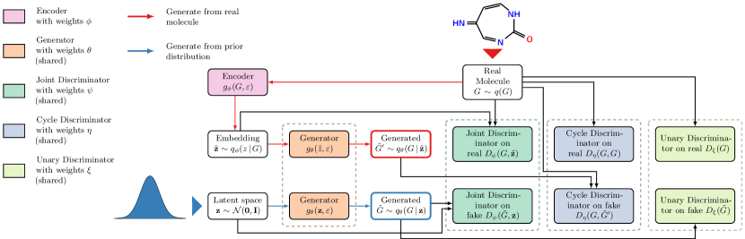
Figure 1: Overview of the proposed ALMGIG model. Boxes with identical background color represent neural networks that share their weights. The joint discriminator plays a similar role as the discriminator in standard GANs. The cycle discriminator enforces the reconstruction property without explicitly computing a reconstruction loss. Molecules can be generated by transforming a sample from a simple prior distribution (blue path), or by embedding a real molecule into the latent space and reconstructing it (red path).

With respect to the generative model, most previous work use either VAEs or adversarial learning. VAEs and AAEs take a molecule representation as input and project it via an inference model (encoder) to a latent space, which is subsequently transformed by a decoder to produce a molecule representation [2, 5, 9, 15, 16, 18, 24, 25, 36, 38]. New molecules can be generated by drawing points from a simple prior distribution over the latent space (usually Gaussian) and feeding it to the decoder. AAEs [2, 16] perform variational inference by adversarial learning, using a discriminator as in GANs, which allows using a more complex prior distribution over the latent space. Both VAEs and AAEs are trained to minimize a reconstruction loss, which is expensive to compute. Standard GANs for molecule generation lack an encoder and a reconstruction loss, and are trained via a two-player game between a generator and discriminator [6, 11, 32]. The generator transforms a simple input distribution into a distribution in the space of molecules, such that the discriminator is unable to distinguish between real molecules in the training data and generated molecules. Without an inference model, GANs cannot be used for neighborhood search in the latent space.

3 Methods

We represent molecules as graphs and propose our Adversarial Learned Molecular Graph Inference and Generation (ALMGIG) framework to learn a distribution in the space of molecules, generate novel molecules, and efficiently search the neighborhood of existing molecules. ALMGIG is a bidirectional GAN that has a GCN-based encoder that projects a graph into the latent space and a decoder that outputs a one-hot representation of atoms and an adjacency matrix defining atomic bonds. Hence, graph generation is performed in a single step, which allows considering global properties of a molecule. An undirected multi-graph $G=(\mathcal{V},\mathcal{R},\mathcal{E})$ is defined by its vertices $\mathcal{V}=\{v_{1},\ldots,v_{n}\}$, relation types $\mathcal{R}=\{r_{1},\ldots,r_{m}\}$, and typed edges (relations) $\mathcal{E}=\{(v_{i},r_{k},v_{j})\,|\,v_{i},v_{j}\in\mathcal{V},r_{k}\in\mathcal{R}\}$. Here, we only allow vertices to be connected by at most one type of edge. We represent a multi-graph $G$ by its adjacency tensor $\mathbf{A}\in\{0,1\}^{n\times n\times m}$, where $A_{ijk}$ is one if $(v_{i},r_{k},v_{j})\in\mathcal{E}$ and zero otherwise, and the node feature matrix $\mathbf{X}=\left(\mathbf{x}_{v_{1}},\ldots,\mathbf{x}_{v_{n}}\right)^{\top}\in\mathbb{R}^{n\times d}$, where $d$ is the number of features describing each node. Here, vertices are atoms, $\mathcal{R}$ is the set of bonds considered (single, double, triple), and node feature vectors $\mathbf{x}_{v_{i}}$ are one-hot encoded atom types (carbon, oxygen, …), with $d$ representing the total number of atom types. We do not model hydrogen atoms, but implicitly add hydrogens to match an atom’s valence.

3.1 Adversarially Learned Inference

We first describe Adversarially Learned Inference with Conditional Entropy (ALICE) [20], which is at the core of ALMGIG and has not been used for de novo chemical design before. It allows training our encoder-decoder model fully adversarially and implicitly enforces the reconstruction property without the need to compute a reconstruction loss (see overview in fig. 1). It has two generative models: (i) the encoder maps graphs into the latent space, and (ii) the decoder inverts this transformation by mapping latent codes to graphs. Training is performed by matching joint distributions over graphs $G\in\mathcal{G}$ and latent variables $\mathbf{z}\in\mathcal{Z}$. Let $q(G)$ be the marginal data distribution, from which we have samples, $\tilde{\mathbf{z}}$ a latent representation produced by the encoder, and $\tilde{G}$ a generated graph. The encoder generative model over the latent variables is $q_{\phi}(z\,|\,G)$ with parameters $\phi$, and the decoder generative model over graphs is $q_{\theta}(G\,|\,z)$, parametrized by $\theta$. Putting everything together, we obtain the encoder joint distribution $q_{\phi}(G,z)=q(G)q_{\phi}(z\,|\,G)$, and the decoder joint distribution $p_{\theta}(G,z)=p_{z}(z)q_{\theta}(G\,|\,z)$. The objective of Adversarially Learned Inference is to match the two joint distributions [7]. A discriminator network $D_{\psi}$ with parameters $\psi$ is trained to distinguish samples $(G,\tilde{\mathbf{z}})\sim q_{\phi}(G,z)$ from $(\tilde{G},\mathbf{z})\sim p_{\theta}(G,z)$. Drawing samples $\tilde{\mathbf{z}}$ and $\tilde{G}$ is made possible by specifying the encoder $q_{\phi}$ and decoder $q_{\theta}$ as neural networks using the change of variable technique: $\tilde{\mathbf{z}}=g_{\phi}(G,\varepsilon)$, $\tilde{G}=g_{\theta}(\mathbf{z},\varepsilon)$, where $\varepsilon$ is some random source of noise. The objective then becomes the following min-max game:

$$\begin{split}\min_{\theta,\phi}\max_{\psi}\quad&\mathbb{E}_{G\sim q(G),~{}\tilde{\mathbf{z}}\sim q_{\phi}(z\,|\,G)}[\log\sigma(D_{\psi}(G,\tilde{\mathbf{z}}))]\\ &+\mathbb{E}_{\tilde{G}\sim q_{\theta}(G\,|\,z),~{}\mathbf{z}\sim p(z)}[\log(1-\sigma(D_{\psi}(\tilde{G},\mathbf{z})))].\end{split}$$ (1)

where $\sigma(\cdot)$ denotes the sigmoid function. At the optimum of (1), the marginal distributions $q_{\theta}(G\,|\,z)$ and $q_{\phi}(z\,|\,G)$ will match, but their relationship can still be undesirable. For instance, the decoder $g_{\theta}(\mathbf{z},\varepsilon)$ could map a given $z$ to $G_{1}$ half of the time and to a distinct $G_{2}$ the other half of the time – the same applies to the encoder [20]. ALICE [20] solves this issue by including a cycle-consistency constraint via an additional adversarial loss. This encourages encoder and decoder to mimic the reconstruction property without explicitly solving a computationally demanding graph isomorphism problem. To this end, a second discriminator with parameters $\eta$ is trained to distinguish a real from a reconstructed graph:

$$\begin{split}\min_{\theta,\phi}\max_{\eta}\quad&\mathbb{E}_{G\sim q(G)}[\log\sigma(D_{\eta}(G,G))]\\ &+\mathbb{E}_{\tilde{G}^{\prime}\sim q_{\theta}(G\,|\,\tilde{z}),~{}\tilde{\mathbf{z}}\sim q_{\phi}(z\,|\,G)}[\log(1-\sigma(D_{\eta}(G,\tilde{G}^{\prime})))].\end{split}$$ (2)

While encoder and decoder in ALICE have all the desired properties at the optimum, we rarely find the global optimum, because both are deep neural networks. Therefore, we extend ALICE by including a unary discriminator $D_{\xi}$ only on graphs, as in standard GANs. This additional objective facilitates generator training when the joint distribution is difficult to learn:

$$\begin{split}\min_{\theta,\phi}\max_{\xi}\quad&\mathbb{E}_{G\sim q(G)}[\log\sigma(D_{\xi}(G))]\\ &+\mathbb{E}_{\tilde{G}\sim q_{\theta}(G\,|\,z),~{}\mathbf{z}\sim p(z)}[\log(1-\sigma(D_{\xi}(\tilde{G})))].\end{split}$$ (3)

We will demonstrate in our ablation study that this is indeed essential.

During training, we concurrently optimize (1), (2), and (3) by first updating $\theta$ and $\phi$, while keeping $\psi$, $\eta$ and $\xi$ fixed, and then the other way around. We use a higher learning rate when updating encoder and decoder weights $\theta$, $\phi$ as proposed in [13]. Finally, we employ the 1-Lipschitz constraint in [12] such that discriminators $D_{\psi}$, $D_{\eta}$, and $D_{\xi}$ are approximately 1-Lipschtiz continuous. Next, we will describe the architecture of the encoder, decoder, and discriminators.

3.2 Generator

Adjacency matrix (bonds) and node types (atoms) of a molecular graph are discrete structures. Therefore, the generator must define an implicit discrete distribution over edges and node types, which differs from traditional GANs that can only model continuous distributions. We overcome this issue by using the Gumbel-softmax trick similar to [6]. The generator network $g_{\theta}(\mathbf{z},\varepsilon)$ takes a point $\mathbf{z}$ from latent space and noise $\varepsilon$, and outputs a discrete-valued and symmetric graph adjacency tensor $\mathbf{A}$ and a discrete-valued node feature matrix $\mathbf{X}$. We use an MLP with three hidden layers with 128, 256, 512 units and $\tanh$ activation, respectively. To facilitate better gradient flow, we employ skip-connections from $\mathbf{z}$ to layers of the MLP. First, the latent vector $\mathbf{z}$ is split into three equally-sized parts $\mathbf{z}_{1},\mathbf{z}_{2},\mathbf{z}_{3}$. The input to the first hidden layer is the concatenation $[\mathbf{z}_{1},\varepsilon]$, its output is concatenated with $\mathbf{z}_{2}$ and fed to the second layer, and similarly for the third layer with $\mathbf{z}_{3}$.

We extend $\mathbf{A}$ and $\mathbf{X}$ to explicitly model the absence of edges and nodes by introducing a separate ghost-edge type and ghost-node type. This will enable us to encourage the generator to produce chemically valid molecular graphs as described below. Thus, we define $\tilde{\mathbf{A}}\in\{0,1\}^{n\times n\times(m+1)}$ and $\tilde{\mathbf{X}}\in\{0,1\}^{n\times(d+1)}$. Each vector $\tilde{\mathbf{A}}_{ij\bullet}$, representing generated edges between nodes $i$ and $j$, needs to be a member of the simplex $\Delta^{m}=\{(y_{0},y_{1},\ldots,y_{m})\,|\,y_{k}\in\{0,1\},\sum_{k=0}^{m}y_{k}=1\}$, because only none or a single edge between $i$ and $j$ is allowed. Here, we use the zero element to represent the absence of an edge. Similarly, each generated node feature vector $\tilde{\mathbf{x}}_{v_{i}}$ needs to be a member of the simplex $\Delta^{d}$, where the zero element represents ghost nodes.

Gumbel-softmax Trick.

The generator is a neural network with two outputs, $\mathrm{MLP}_{A}(\mathbf{z})\in\mathbb{R}^{n\times n\times(m+1)}$ and $\mathrm{MLP}_{X}(\mathbf{z})\in\mathbb{R}^{n\times(d+1)}$, which are created by linearly projecting hidden units into a $n^{2}(m+1)$ and $n(d+1)$ dimensional space, respectively. Next, continuous outputs need to be transformed into discrete values according to the rules above to obtain tensors $\tilde{\mathbf{A}}$ and $\tilde{\mathbf{X}}$ representing a generated graph. Since the argmax operation is non-differentiable, we employ the Gumbel-softmax trick [14, 27], which uses reparameterization to obtain a continuous relaxation of discrete states. Thus, we obtain an approximately discrete adjacency tensor $\tilde{\mathbf{A}}$ from $\mathrm{MLP}_{A}(\mathbf{z})$, and feature matrix $\tilde{\mathbf{X}}$ from $\mathrm{MLP}_{X}(\mathbf{z})$.

Node Connectivity and Valence Constraints.

While this allows us to generate graphs with varying number of nodes, the generator could in principle generate graphs consisting of two or more separate connected components. In addition, generating molecules where atoms have the correct number of shared electron pairs (valence) is an important aspect the generator needs to consider, otherwise generated graphs would represent invalid molecules. Finally, we want to prohibit edges between any pair of ghost nodes. All of these issues can be addressed by incorporating regularization terms proposed in [26]. Multiple connected components can be avoided by generating graphs that have a path between every pair of non-ghost nodes. Using the generated tensor $\tilde{\mathbf{A}}$, which explicitly accounts for ghost edges, the number of paths between nodes $i$ and $j$ is given by

$$\textstyle\tilde{\mathbf{B}}_{ij}=I(i=j)+\sum_{k=1}^{m}\sum_{p=1}^{n-1}\left(\tilde{\mathbf{A}}^{p}\right)_{ijk}.$$ (4)

The regularizer comprises two terms, the first term encourages non-ghost nodes $i$ and $j$ to be connected by a path, and the second term that a ghost node and non-ghost node remain disconnected:

$$\textstyle\frac{\mu}{n^{2}}\sum_{i,j}\left[1-\left(\tilde{\mathbf{x}}_{v_{i}}\right)_{0}\right]\left[1-\left(\tilde{\mathbf{x}}_{v_{j}}\right)_{0}\right]\left[1-\tilde{\mathbf{B}}_{ij}\right]+\frac{\mu}{n^{2}}\left(\tilde{\mathbf{x}}_{v_{i}}\right)_{0}\left(\tilde{\mathbf{x}}_{v_{j}}\right)_{0}\tilde{\mathbf{B}}_{ij},$$ (5)

where $\mu$ is a hyper-parameter, and $\left(\tilde{\mathbf{x}}_{v_{i}}\right)_{0}>0$ if the $i$-th node is a ghost node.

To ensure atoms have valid valence, we enforce an upper bound – hydrogen atoms are modeled implicitly – on the number of edges of a node, depending on its type (e.g. four for carbon). Let $\mathbf{u}=(u_{0},u_{1},\ldots,u_{d})^{\top}$ be a vector indicating the maximum capacity (number of bonding electron pairs) a node of a given type can have, where $u_{0}=0$ denotes the capacity of ghost nodes. The vector $\mathbf{b}=(b_{0},b_{r_{1}},\ldots,b_{r_{m}})$ denotes the capacity for each edge type with $b_{0}=0$ representing ghost edges. The actual capacity of a node $v_{i}$ can be computed by $c_{v_{i}}=\sum_{j\neq i}\mathbf{b}^{\top}\tilde{\mathbf{A}}_{ij\bullet}.$ If $c_{v_{i}}$ exceeds the value in $\mathbf{u}$ corresponding to the node type of $v_{i}$, the generator incurs a penalty. The valence penalty with hyper-parameter $\nu>0$ is defined as

$$\frac{\nu}{n}\sum_{i=1}^{n}\max(0,c_{v_{i}}-\mathbf{u}^{\top}\tilde{\mathbf{x}}_{v_{i}}).$$ (6)

3.3 Encoder and Discriminators

The architecture of the encoder $g_{\phi}(G,\varepsilon)$, and the three discriminators $D_{\psi}(G,\mathbf{z})$, $D_{\eta}(G_{1},G_{2})$, and $D_{\xi}(G)$ are closely related, because they all take graphs as input. First, we extract node-level descriptors by stacking several GCN layers. Next, node descriptors are aggregated to obtain a graph-level descriptor, which forms the input to a MLP. Here, inputs are multi-graphs with $m$ edge types, which we model by extending the Graph Isomorphism Network (GIN) architecture [39] to multi-graphs. Let $\mathbf{h}_{v_{i}}^{(l+1)}$ denote the descriptor of node $v_{i}$ after the $l$-th GIN layer, with $\mathbf{h}_{v_{i}}^{(0)}=\mathbf{x}_{v_{i}}$, then node descriptors get updated as follows:

$$\textstyle\mathbf{h}_{v_{i}}^{(l+1)}=\tanh\left[\sum_{k=1}^{m}\mathrm{MLP}_{r_{k}}^{(l)}\left((1+\epsilon^{(l)})\mathbf{h}_{v_{i}}^{(l)}+\sum_{u\in\mathcal{N}_{r_{k}}(v_{i})}\mathbf{h}_{u}^{(l)}\right)\right],$$ (7)

where $\epsilon^{(l)}\in\mathbb{R}$ is a learnable weight, and $\mathcal{N}_{r_{k}}(v_{i})=\{u\,|\,(u,r_{k},v_{i})\in\mathcal{E}\}$. Next, graph-level node aggregation is performed. We use skip connections [40] to aggregate node-level descriptors from all $L$ GIN layers and soft attention [22] to allow the network to learn which node descriptors to use. The graph-level descriptor $\mathbf{h}_{G}$ is defined as

$$\mathbf{h}_{v_{i}}^{c} =\mathrm{CONCAT}(\mathbf{x}_{v_{i}},\mathbf{h}_{v_{i}}^{(1)}\ldots,\mathbf{h}_{v_{i}}^{(L)}),$$ (8)

$$\mathbf{h}_{v_{i}}^{c^{\prime}} =\tanh(\mathbf{W}_{1}\mathbf{h}_{v_{i}}^{c}+\mathbf{b}_{1}), \mathbf{h}_{G}=\textstyle\sum_{v\in\mathcal{V}}\sigma(\mathbf{W}_{2}\mathbf{h}_{v}^{c^{\prime}}+\mathbf{b}_{2})\odot\mathbf{h}_{v}^{c^{\prime}},$$ (9)

where $\mathbf{W}$ and $\mathbf{b}$ are parameters to be learned. Graph-level descriptors can be abstracted further by adding an additional MLP on top, yielding $\mathbf{h}_{G}^{\prime}$. The discriminator $D_{\xi}(G)$ contains a single GIN module, $D_{\eta}(G_{1},G_{2})$ contains two GIN modules to extract descriptors $\mathbf{h}_{G_{1}}^{\prime}$ and $\mathbf{h}_{G_{2}}^{\prime}$, which are combined by component-wise multiplication and fed to a 2-layer MLP. $D_{\psi}(G,\mathbf{z})$ has a noise vector as second input, which is the input to an MLP whose output is concatenated with $\mathbf{h}_{G}^{\prime}$ and linearly projected to form $\log[\sigma(D_{\psi}(G,\mathbf{z}))]$. The encoder $g_{\phi}(G,\varepsilon)$ is identical to $D_{\psi}(G,\mathbf{z})$, except that its output matches the dimensionality of $\mathbf{z}$.

4 Evaluation Metrics

To evaluate generated molecules, we adapted the metrics proposed in [4]: the proportion of valid, unique, and novel molecules, and a comparison of 10 physicochemical descriptors to assess whether new molecules have similar chemical properties as the reference data. Validity is the percentage of molecular graphs with a single connected component and correct valence for all its nodes. Uniqueness is the percentage of unique molecules within a set of $N$ randomly sampled valid molecules. Novelty is the percentage of molecules not in the training data within a set of $N$ unique randomly sampled molecules. Validity and novelty are percentages with respect to the set of valid and unique molecules, which we obtain by repeatedly sampling $N$ molecules (up to 10 times). Models that do not generate $N$ valid/unique molecules will be penalized. To measure to which extent a model is able to estimate the distribution of molecules from the training data, we first compute the distribution of 10 chemical descriptors $d_{k}$ used in [4]. Internal similarity is a measure of diversity that is defined as the maximum Tanimoto similarity with respect to all other molecules in the dataset – using the binary Extended Connectivity Molecular Fingerprints with diameter 4 (ECFP4) [34]. The remaining descriptors measure physicochemical properties of molecules (see fig. 4 for a full list).

For each descriptor, we compute the difference between the distribution with respect to generated molecules ($Q$) and the reference data ($P$) using the 1-Wasserstein distance. This is in contrast to [4], who use the Kullback-Leibler (KL) divergence $D_{\text{KL}}(P\parallel Q)$. Using the KL divergence has several drawbacks: (i) it is undefined if the support of $P$ and $Q$ do not overlap, and (ii) it is not symmetric. Due to the lack of symmetry, it makes a big difference whether $Q$ has a bigger support than $P$ or the other way around. Most importantly, an element outside of the support of $P$ is not penalized, therefore $D_{\text{KL}}(P\parallel Q)$ will remain unchanged whether samples of $Q$ are just outside of the support of $P$ or far away.

The 1-Wasserstein distance, also called Earth Mover’s Distance (EMD), is a valid metric and does not have this undesirable properties. It also offers more flexibility in how out-of-distribution samples are penalized by choosing an appropriate ground distance (e.g. Euclidean distance for quadratic penalty, and Manhattan distance for linear penalty). We approximate the distribution on the reference data and the generated data using histograms $\mathbf{h}_{k}^{\text{ref}}$ and $\mathbf{h}_{k}^{\text{gen}}$, and define the ground distance $\mathbf{C}_{ij}(k)$ between the edges of the $i$-th and $j$-th bin as the Euclidean distance, normalized by the minimum of the standard deviation of descriptor $d_{k}$ on the reference and the generated data. As overall measure of how well properties of generated molecules match those of molecules in the reference data, we compute the mEMD, defined as

$$\mathrm{mEMD}(\mathbf{h}_{k}^{\text{ref}},\mathbf{h}_{k}^{\text{gen}}) ={\textstyle\frac{1}{10}\sum_{k=1}^{10}\exp[-\mathrm{EMD}(\mathbf{h}_{k}^{\text{ref}},\mathbf{h}_{k}^{\text{gen}})],}$$ (10)

$$\mathrm{EMD}(\mathbf{h}_{k}^{\text{ref}},\mathbf{h}_{k}^{\text{gen}}) ={\textstyle\min_{\mathbf{P}\in\mathbf{U}(\mathbf{h}_{k}^{\text{ref}},\mathbf{h}_{k}^{\text{gen}})}\langle\mathbf{C}(k),\mathbf{P}\rangle,}$$ (11)

where $\mathbf{U}(\mathbf{a},\mathbf{b})$ is the set of coupling matrices with $\mathbf{P}{\mathchoice{\rm 1\mskip-4.0mul}{\rm 1\mskip-4.0mul}{\rm 1\mskip-4.5mul}{\rm 1\mskip-5.0mul}}=\mathbf{a}$ and $\mathbf{P}^{\top}{\mathchoice{\rm 1\mskip-4.0mul}{\rm 1\mskip-4.0mul}{\rm 1\mskip-4.5mul}{\rm 1\mskip-5.0mul}}=\mathbf{b}$ [35]. A perfect model with $\mathrm{EMD}=0$ everywhere would obtain a mEMD score of 1.

5 Experiments

In our experiments, we use molecules from the QM9 dataset [33] with at most 9 heavy atoms. We consider $d=4$ node types (atoms C, N, O, F), and $m=3$ edge types (single, double, and triple bonds). After removal of molecules with non-zero formal charge, we retained $131\,941$ molecules, which we split into 80% for training, 10% for validation, and 10% for testing.

We extensively compare ALMGIG against three state-of-the-art VAEs: NeVAE [36] and CGVAE [25] are graph-based VAEs with validity constraints, while GrammarVAE [18] uses the SMILES representation. We also compare against MolGAN [6], which is a Wasserstein GAN without inference network, reconstruction loss, node connectivity, or valence constraints. Finally, we include a random graph generation model, which only enforces valence constraints during generation, similar to CGVAE and NeVAE, but selects node types ($\mathbf{X}$) and edges ($\mathbf{A}$) randomly. Note that generated graphs can have multiple connected components if valence constraints cannot be satisfied otherwise; we consider these to be invalid. For NeVAE, we use our own implementation, for the remaining methods, we use the authors’ publicly available code. Further details are described in supplement 0.B.

5.1 Latent Space

(a)

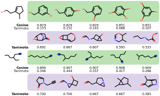
(b)
Reconstructed (%) Generated (%) Ghost-node bond 0  (0.00) 2  (0.02) Valency 17  (0.13) 36  (0.28) Split graph 296  (2.31) 686  (5.36) Valid $12\,487$ (97.55) $12\,076$ (94.34)

Figure 2: (a) Nearest neighbors with respect to the molecule in the first column in embedding space (green rows) and according to Tanimoto similarity (purple rows). (b) Frequency of errors of ALMGIG on test set.

In the first experiment, we investigate properties of the encoder and the associated latent space. We project molecules of the test set into the latent space, and perform a $k$ nearest neighbor search to find the closest latent representation of a molecule in the training set in terms of cosine distance. We compare results against the nearest neighbors by Tanimoto similarity of ECFP4 fingerprints [34]. Figure 2a shows that the two approaches lead to quite different sets of nearest neighbors. Nearest neighbors based on molecules’ latent representation usually differ by small substructures. For instance, the five nearest neighbor in the first row of fig. 2a differ by the location of side chains around a shared ring structure. On the other hand, the topology of nearest neighbors by Tanimoto similarity (second row) differs considerably from the query. Moreover, all but one nearest neighbor contain nitrogen atoms, which are absent from the query. In the second example (last two rows), the nearest neighbors in latent space are all linear structures with one triple bond and nitrogen, whereas all nearest neighbors by Tanimoto similarity contain ring structures and only one contains a triple bond. Additional experiments with respect to interpolation in the latent space can be found in supplement 0.A.1.

5.2 Molecule Generation

Next, we evaluate the quality of generated molecules. We generate molecules from $N=$10\,000$$ latent vectors, sampled from a unit sphere Gaussian and employ the metrics described in section 4. Note that previous work defined uniqueness and novelty as the percentage with respect to all valid molecules rather than $N$, which is hard to interpret, because models with low validity would have high novelty. Hence, percentages reported here are considerably lower.

Figure 3a shows that ALMGIG generates molecules with high validity (94.9%) and is only outperformed by CGVAE, which by design is constrained to only generate valid molecules, but has ten times more parameters than ALMGIG (1.1M vs. 13M). Moreover, ALMGIG ranks second in novelty and third in uniqueness (excluding random); we will investigate the reason for this difference in detail in the next section on distribution learning. Graph-based NeVAE always generates molecules with correct valence, but often (88.2%) generates graphs with multiple connected components, which we regard as invalid. Its set of valid generated molecules has the highest uniqueness. We can also observe that graph-based models outperform the SMILES-based GrammarVAE, which is prone to generate invalid SMILES representation of molecules, which is a known problem [2, 11, 24, 32, 37]. MolGAN is a regular GAN without inference network. It is struggling to generate molecules with valid valence and only learned one particular mode of the distribution, which we will discuss in more detail in the next section. It is inferior to ALMGIG in all categories, in particular with respect to novelty and uniqueness of generated molecules.

Next, we inspect the reason for generated molecules being invalid to assess whether imposed node connectivity and valence constraints are effective. Molecules can be generated by (a) reconstructing the latent representation of a real molecule in the test set, or (b) by decoding a random latent representation draw from an isotropic Gaussian (see fig. 1). Figure 2b reveals that most errors are due to multiple disconnected graphs being generated (2-5%). While individual components do represent valid molecules, we treat them as erroneous molecular graphs. In these instances, 98-99% of graphs have 2 connected components and the remainder has 3. Less than 0.3% of molecules have atoms with improper valence and less than 0.1% of graphs have atomic bonds between ghost nodes. Therefore, we conclude that the constraints are highly effective.

(a)

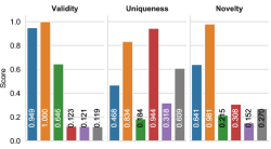
(b)

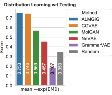
Figure 3: (a) Overview of simple molecule generation statistics. (b) Comparison with respect to the proposed mEMD evaluation metric for distribution learning. See figs. 4 and 0.A.2 for differences between individual distributions.

Finally, we turn to the random graph generation model. It achieves a relatively high uniqueness of 60.9%, which ranks third, and has a higher novelty than MolGAN and GrammarVAE. Many generated graphs have multiple connected components, which yields a low validity. The fact that the random model cannot be clearly distinguished from trained models, indicates that validity, uniqueness, and novelty do not accurately capture what we are really interested in: Can we generate chemically meaningful molecules with similar properties as in the training data? We will investigate this question next.

5.3 Distribution Learning

While the simple overall statistics in the previous section can be useful rough indicators, they ignore the physicochemical properties of generated molecules and do not capture to which extent a model is able to estimate the distribution of molecules from the training data. Therefore, we compare the distribution of 10 chemical descriptors in terms of EMD (11). Distributions of individual descriptors are depicted in fig. 4 and fig. 0.A.2 of the supplement.

First of all, we want to highlight that using the proposed mEMD score, we can easily identify the random model (see fig. 3b), which is not obvious from the simple summary statistics in fig. 3a. In particular, from fig. 3a we could have concluded that NeVAE is only marginally better than the random model. The proposed scheme clearly demonstrates that NeVAE is superior to the random model (overall score 0.457 vs 0.350). Considering differences between individual descriptors reveals that randomly generated molecules are not meaningful due to higher number of hydrogen acceptors, molecular weight, molecular complexity, and polar surface area (see fig. 0.A.2d).

(a)

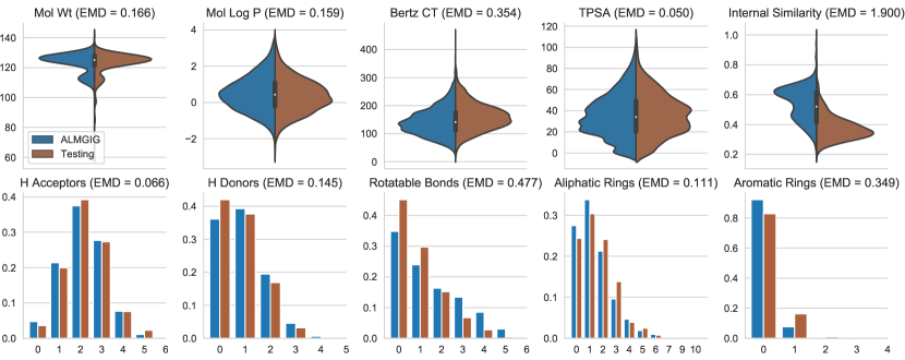
(b)

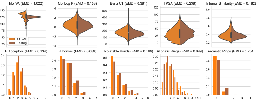
Figure 4: Distribution of chemical properties of the test data and of 10,000 unique molecules generated by (a) ALMGIG, and (b) CGVAE [25]. Mol Wt: molecular weight. Mol Log P: water-octanol partition coefficient. Bertz CT: molecular complexity index. TPSA: molecular polar surface area. H Acceptors (Donors): Number of hydrogen acceptors (donors).

ALMGIG achieves the best overall mEMD score, with molecular weight and polar surface area best matching that of the test data by a large margin (EMD = 0.17 and 0.05, see fig. 4a). The highest difference is due to the internal similarity of generated molecules (EMD = 1.90). Among all VAEs, CGVAE is performing best (see fig. 4b). However, it notably produces big molecules with larger weight (EMD = 1.02) and lower polar surface area (EMD = 0.238). The former explains its high novelty value in fig. 3a: by creating bigger molecules than in the data, a high percentage of generated molecules is novel and unique. Molecules generated by NeVAE (see fig. 0.A.2a) have issues similar to CGVAE: they have larger weight (EMD = 1.72) and higher polar surface area (EMD = 0.839), which benefits uniqueness. In contrast to ALMGIG and CGVAE, it also struggles to generate molecules with aromatic rings (EMD = 0.849). GrammarVAE in fig. 0.A.2b is far from capturing the data distribution, because it tends to generate long SMILES strings corresponding to heavy molecules (EMD = 5.66 for molecular weight). Molecules produced by MolGAN are characterized by a striking increase in internal similarity without any overlap with the reference distribution (EMD = 6.41; fig. 0.A.2c). This result is an example where comparison by KL divergence would be undefined. An interesting detail can be derived from the distribution of molecular weight: MolGAN has problems generating molecules with intermediate to low molecular weight ($<115$ g/mol), which highlights a common problem with GANs, where only one mode of the distribution is learned by the model (mode collapse). In contrast, ALMGIG can capture this mode, but still misses the smaller mode with molecular weight below 100 g/mol (see fig. 4a). This mode contains only $2344$ molecules (2.2%), which makes it challenging – for any model – to capture. This demonstrates that our proposed Wasserstein-based evaluation can reveal valuable insights that would have been missed when solely relying on validity, novelty, and uniqueness.

5.4 Ablation Study

Table 1: Configurations evaluated in our ablation study. SC: Skip-connections.

	Penalties		Discriminators			Architecture
	Conn.	Valence	Unary	Joint	Cycle	GIN SC	Gen. SC	Attention
ALMGIG	✓	✓	✓	✓	✓	✓	✓	✓
No Connectivity	✗	✓	✓	✓	✓	✓	✓	✓
No Valence	✓	✗	✓	✓	✓	✓	✓	✓
No Conn+Valence	✗	✗	✓	✓	✓	✓	✓	✓
No GIN SC	✓	✓	✓	✓	✓	✗	✓	✓
No Generator SC	✓	✓	✓	✓	✓	✓	✗	✓
No Attention	✓	✓	✓	✓	✓	✓	✓	✗
ALICE	✓	✓	✗	✓	✓	✓	✓	✓
ALI	✓	✓	✗	✓	✗	✓	✓	✓
(W)GAN	✓	✓	✓	✗	✗	✓	✓	✓

Next, we evaluate a number of modeling choices by conducting an extensive ablation study (see table 1). We first evaluate the impact of the connectivity (5) and valence penalty (6) during training. Next, we evaluate architectural choices, namely (i) skip connections in the GIN of encoder and discriminators, (ii) skip connections in the generator, and (iii) soft attention in the graph pooling layer (8). Finally, we use the proposed architecture and compared different adversarial learning schemes: ALI [7], ALICE [20], and a traditional WGAN without an encoder network $g_{\phi}(G,\varepsilon)$ [1, 10]. Note that WGAN is an extension of MolGAN [6] with connectivity and valence penalties, and GIN-based architecture.

Our results are summarized in fig. 5 (details in fig. 0.A.3 of the supplement). As expected, removing valence and connectivity penalties lowers the validity, whereas the drop when only removing the valence penalty is surprisingly small, but does lower the uniqueness considerably. Regarding our architectural choices, results demonstrate that only the proposed architecture of ALMGIG is able to generate a sufficient number of molecules with aromatic rings (EMD = 0.35), when removing the attention mechanism (EMD = 0.96), skip connections from the GIN (EMD = 0.74), or from the generator (EMD = 1.26) the EMD increases at least two-fold. When comparing alternative adversarial learning schemes, we observe that several configurations resulted in mode collapse. It is most obvious for ALI, GAN, and WGAN, which can only generate a few molecules and thus have very low uniqueness and novelty. In particular, ALI and WGAN are unable to generate molecules with aromatic rings. ALICE is able to generate more diverse molecules, but is capturing only a single mode of the distribution: molecules with low to medium weight are absent. This demonstrates that including a unary discriminator, as in ALMGIG, is vital to capture the full distribution over chemical structures. Finally, it is noteworthy that WGAN, using our proposed combination of GIN architecture and penalties, outperforms MolGAN [6]. This demonstrates that our proposed architecture can already improve existing methods for molecule generation considerably. When also extending the adversarial learning framework, the results demonstrate that ALMGIG can capture the underlying distribution of molecules more accurately than any competing method.

(a)

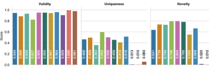
(b)

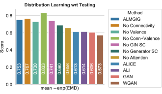
Figure 5: Results of ablation study. (a) Simple molecule generation statistics. (b) Comparison with respect to the proposed mEMD evaluation metric for distribution learning.

6 Conclusion

We formulated generation and inference of molecular graphs as a likelihood-free adversarial learning task. Compared to previous work, it allows training without explicitly computing a reconstructing loss, which would require solving an expensive graph isomorphism problem. Moreover, we argued that the common validation metrics validity, novelty, and uniqueness are insufficient to properly assess the performance of algorithms for molecule generation, because they ignore physicochemical properties of generated molecules. Instead, we proposed to compute the 1-Wasserstein distance between distributions of physicochemical properties of molecules. We showed that the proposed adversarial learning framework for molecular graph inference and generation, ALMGIG, allows efficiently exploring the space of molecules via molecules’ continuous latent representation, and that it more accurately represents the distribution over the space of molecules than previous methods.

Acknowledgements

This research was partially supported by the Bavarian State Ministry of Education, Science and the Arts in the framework of the Centre Digitisation.Bavaria (ZD.B), and the Federal Ministry of Education and Research in the call for Computational Life Sciences (DeepMentia, 031L0200A). We gratefully acknowledge the support of NVIDIA Corporation with the donation of the Quadro P6000 GPU used for this research.

Appendix 0.A Additional Results

0.A.1 Latent Space Interpolation

In this experiment, we interpolate between two molecules by computing their respective latent representation $\tilde{\mathbf{z}}_{A}$ and $\tilde{\mathbf{z}}_{B}$ and reconstructing molecules from latent codes on the line between $\tilde{\mathbf{z}}_{A}$ and $\tilde{\mathbf{z}}_{B}$. The results are depicted in fig. 0.A.1. Interpolation between molecules appears smooth, but we can also see examples of latent representations corresponding to graphs with multiple connected components (second to last row), which we excluded from our analyses above, but included here for illustration.

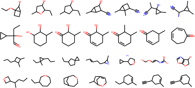
Figure 0.A.1: Each row is a one-dimensional interpolation in latent space. The left and right most molecule are from the QM9 data, the remaining molecules lie on the line from the latent representation of the left most to the right most molecule.

0.A.2 Distribution Learning

Figure 0.A.2: Distribution of 10 descriptors of molecules in the test data and of 10,000 unique molecules generated by (a) NeVAE [36], (b) GrammarVAE [18], (c) MolGAN [6], and (d) randomly.

(a)

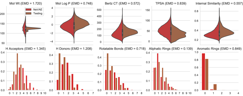
(b)

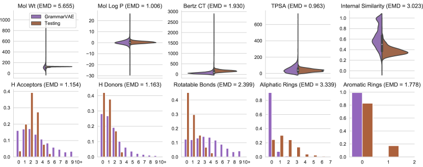
(c)

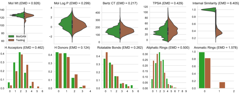
(d)

Figure 0.A.3: Distribution of 10 descriptors of molecules in the test data and of 10,000 unique generated molecules used in ablation study.

(a)

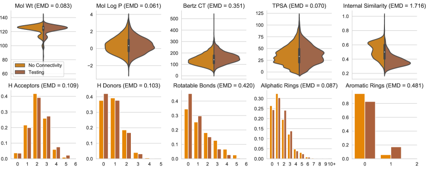
(b)

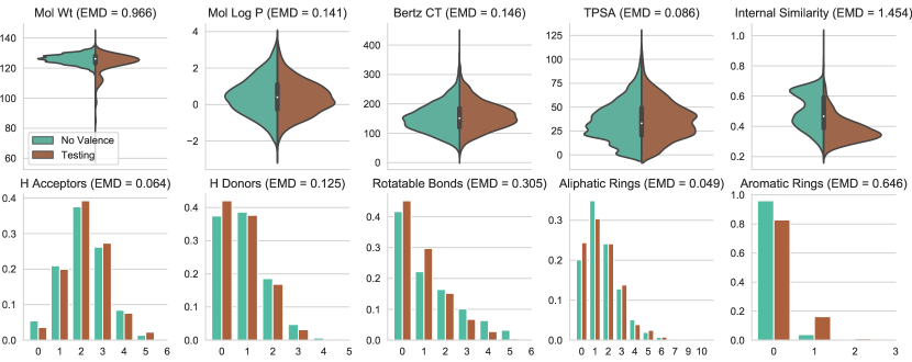
(c)

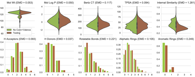
(d)

(e)

(f)

(g)

(h)

(i)

(j)

Appendix 0.B Implementation Details

Table 0.B.1: Number of learnable weights for each model.

Model	Parameters
ALMGIG	1.11M
No Encoder Skip-Conn.	1.03M
No Generator Skip-Conn.	1.10M
No Attention	1.03M
ALICE	987K
ALI	729K
(W)GAN	509K
CGVAE	13.6M
MolGAN	439K
NeVAE	0.5K
GrammarVAE	5.4M

GIN.

We implemented the sum over the descriptors of neighboring nodes in the GIN layer (7) as a dense matrix product between the adjacency matrix $\mathbf{A}_{\bullet,\bullet,r_{k}}$ and the matrix $(\mathbf{h}_{v_{1}}^{(l)},\ldots,\mathbf{h}_{v_{n}}^{(l)})^{\top}$, which has a complexity of $O(n^{2}d)$. Clearly, this is a bottleneck for large graphs. However, due to the sparsity of the adjacency matrix, we can be employ sparse matrix computation. In the first layer, where descriptors are one-hot encoded node types, the computation requires $O(\bar{e})$ operations, with $\bar{e}$ being the average number of edges between nodes. After the second layer, descriptors will be dense and we have to compute the product between a sparse and a dense matrix, which requires $O(\bar{e}d)$ operations. To the best of our knowledge, most deep learning frameworks only support sparse computation on rank-2 matrices, therefore additional engineering would be required to incorporate the batch dimension for efficient sparse matrix computation.

Architecture.

If not mentioned otherwise, tanh is used as activation function. Encoders and discriminators have $L=2$ GIN-layers with 128 units for each of the $m=3$ edge types. The GIN-MLP in (7) has one linear layer. The two linear layers used for soft-attention and subsequent graph-pooling in (8) have 128 units each. The MLP taking the graph-pooled descriptor $\mathbf{h}_{G}$ and outputting $\mathbf{h}_{G}^{\prime}$ has two fully-connected layers with 128 and 64 units, respectively. The cycle-discriminator $D_{\eta}(G_{1},G_{2})$ uses a 2-layer MLP with 64 units each to combine graph-level feature descriptors $\mathbf{h}_{G_{1}}^{\prime}$ and $\mathbf{h}_{G_{2}}^{\prime}$. Networks $D_{\psi}(G,\mathbf{z})$, $g_{\phi}(G,\varepsilon)$ have a 96-dimensional noise vector as second input, which is the input to one fully-connected layer with 256 units. Likewise, $g_{\theta}(\mathbf{z},\varepsilon)$ takes two 96-dimensional vectors; $\mathbf{z}$ is split into three 32-dimensional vectors used in the decoder’s skip connections and $\varepsilon$ is concatenated with $\mathbf{z}_{1}$ and fed to a 3-layer MLP with 128, 256, and 512 units. The hyper-parameter $\tau$ used in the Gumbel-softmax [14, 27] is set to $\tau=1$. We trained for 250 epochs using the Adam optimizer [17] with $\beta_{1}=0.5$, $\beta_{2}=0.9$, with initial learning rates 0.001 and 0.0004 for the generator and discriminator, respectively. We lowered the initial learning rates by a factor of 0.5, 0.1, and 0.01 after 80, 150, and 200 epochs, respectively. The regularization weights $\mu$ and $\nu$ in (5) and (6) were tuned manually and set to $0.005$ and $0.05$. In practice, we compute a smoothed version of $\tilde{\mathbf{B}}_{ij}$ in (4) using $s(x)=\sigma(a(x-\frac{1}{2}))$ with $a=100$, which improves numerical stability. The weight of the gradient penalty [12] of the discriminators was set to 10. Weights $\theta$ and $\phi$ of the encoder and decoder get updated at the same time, as are the weights $\psi$, $\eta$, and $\xi$ of the discriminators. Updates are performed sequentially, with a 1:1 ratio of discriminator to encoder/decoder updates. To stabilize training and encourage exploration, we added a discount term proportional to the variance of the predictions of the discriminator $D_{\psi}(\tilde{G},\mathbf{z})$. The term was weighted by $-0.2$ and added to the remaining losses when updating weights $\theta$ and $\phi$ of the encoder and decoder.

Random Graph Generation.

For the random graph generation model, we used a similar setup as the generator used in NeVAE [36]. We first randomly select the atom types for each node in the graph to create $\mathbf{X}$, and then sequentially draw edges $(v_{i},r_{k},v_{j})$ such that the valence of atoms is always correct. We denote by $\delta(i,j\,|\,\mathcal{E}_{l})\in\{0;1\}$ whether nodes $v_{i}$ and $v_{j}$ are disconnected in the graph specified by the set of edges $\mathcal{E}_{l}$, and by $\delta(r_{k}\,|\,v_{i},v_{j},\mathcal{E}_{l})\in\{0;1\}$ whether nodes $v_{i}$ and $v_{j}$ can be connected by an edge of type $r_{k}$ without violating valence constraints. The first mask is used to ensure only a single bond between atoms is formed, and the second mask to satisfy valence constraints. Independent random noise drawn from $\mathcal{N}(0,1)$ is denoted by $\varepsilon$.

The probability of the $i$-th node feature vector $\mathbf{x}_{v_{i}}$ encoding the atom type is given by

$$P(\mathbf{x}_{v_{i}}=\mathbf{e}_{j})=\frac{\exp{\varepsilon_{j}}}{\sum_{j^{\prime}=1}^{d}\exp{\varepsilon_{j^{\prime}}}},$$

where $\mathbf{e}_{j}$ is the one-hot encoding of the $j$-th atom type ($j=1,\ldots,d$). Edges are added sequentially: in the $l$-th step, the probability of an edge $(v_{i},r_{k},v_{j})$, conditional on the previously added edges $\mathcal{E}_{l-1}$ is given by

$$P((v_{i},r_{k},v_{j})\,|\,\mathcal{E}_{l-1}) =P(v_{i},v_{j}\,|\,\mathcal{E}_{l-1})P(r_{k}\,|\,v_{i},v_{j},\mathcal{E}_{l-1}),$$

$$P(v_{i},v_{j}\,|\,\mathcal{E}_{l-1}) =\frac{\delta(i,j\,|\,\mathcal{E}_{l-1})\exp(\varepsilon_{i,j})}{\sum_{i^{\prime},j^{\prime}}\delta(i^{\prime},j^{\prime}\,|\,\mathcal{E}_{l-1})\exp(\varepsilon_{i^{\prime},j^{\prime}})},$$

$$P(r_{k}\,|\,v_{i},v_{j},\mathcal{E}_{l-1}) =\frac{\delta(r_{k}\,|\,v_{i},v_{j},\mathcal{E}_{l-1})\exp(\varepsilon_{r_{k}})}{\sum_{k^{\prime}=1}^{r}\delta(r_{k^{\prime}}\,|\,v_{i},v_{j},\mathcal{E}_{l-1})\exp(\varepsilon_{r_{k^{\prime}}})}.$$

We repeatedly sample edges until no additional valid edges can be added. Therefore, generated random molecular graphs will always have correct valences, but can have multiple connected components if valence constraints cannot be satisfied otherwise; we consider these samples to be invalid.

Software.

We implemented our model using TensorFlow version 1.10.0 and performed training on a NVIDIA Quadro P6000. We used RDKit [19] version 2018.09.3.0 for computing molecular descriptors. Validity of generated molecular graphs was assessed by RDKit’s SanitizeMol function. To evaluate how well models estimate the distribution of molecules from the training data, we used the benchmark suite GuacaMol version 0.3.2 [4] and the Python Optimal Transport (POT) library version 0.5.1 [8].

References

- [1] Arjovsky, M., Chintala, S., Bottou, L.: Wasserstein Generative Adversarial Networks. In: 34th International Conference on Machine Learning. vol. 70, pp. 214–223 (2017)
- [2] Blaschke, T., Olivecrona, M., Engkvist, O., Bajorath, J., Chen, H.: Application of Generative Autoencoder in De Novo Molecular Design. Molecular Informatics 37(1-2), 1700123 (2018)
- [3] Bradshaw, J., Paige, B., Kusner, M.J., Segler, M., Hernández-Lobato, J.M.: A model to search for synthesizable molecules. In: Advances in Neural Information Processing Systems 32. pp. 7937–7949 (2019)
- [4] Brown, N., Fiscato, M., Segler, M.H., Vaucher, A.C.: GuacaMol: Benchmarking Models for de Novo Molecular Design. Journal of Chemical Information and Modeling 59(3), 1096–1108 (2019)
- [5] Dai, H., Tian, Y., Dai, B., Skiena, S., Song, L.: Syntax-Directed Variational Autoencoder for Structured Data. In: 6th International Conference on Learning Representations (2018)
- [6] De Cao, N., Kipf, T.: MolGAN: An implicit generative model for small molecular graphs (2018), https://arxiv.org/abs/1805.11973
- [7] Dumoulin, V., Belghazi, I., Poole, B., Mastropietro, O., Lamb, A., Arjovsky, M., Courville, A.: Adversarially learned inference. 5th International Conference on Learning Representations (2017)
- [8] Flamary, R., Courty, N.: POT Python Optimal Transport library (2017), https://github.com/rflamary/POT
- [9] Gómez-Bombarelli, R., Wei, J.N., Duvenaud, D., Hernández-Lobato, J.M., Sánchez-Lengeling, B., et al.: Automatic Chemical Design Using a Data-Driven Continuous Representation of Molecules. ACS Central Science 4(2), 268–276 (2018)
- [10] Goodfellow, I., Pouget-Abadie, J., Mirza, M., Xu, B., Warde-Farley, D., Ozair, S., Courville, A., Bengio, Y.: Generative Adversarial Nets. In: Advances in Neural Information Processing Systems 27. pp. 2672–2680 (2014)
- [11] Guimaraes, G.L., Sanchez-Lengeling, B., Outeiral, C., Farias, P.L.C., Aspuru-Guzik, A.: Objective-Reinforced Generative Adversarial Networks (ORGAN) for Sequence Generation Models (2017), https://arxiv.org/abs/1705.10843
- [12] Gulrajani, I., Ahmed, F., Arjovsky, M., Dumoulin, V., Courville, A.: Improved Training of Wasserstein GANs. In: Advances in Neural Information Processing Systems 30. pp. 5767–5777 (2017)
- [13] Heusel, M., Ramsauer, H., Unterthiner, T., Nessler, B., et al.: GANs trained by a two time-scale update rule converge to a local nash equilibrium. In: Advances in Neural Information Processing Systems 30. pp. 6626–6637 (2017)
- [14] Jang, E., Gu, S., Poole, B.: Categorical reparameterization with Gumbel-softmax. In: 5th International Conference on Learning Representations (2017)
- [15] Jin, W., Barzilay, R., Jaakkola, T.: Junction Tree Variational Autoencoder for Molecular Graph Generation. In: 35th International Conference on Machine Learning. pp. 2323–2332 (2018)
- [16] Kadurin, A., Nikolenko, S., Khrabrov, K., Aliper, A., Zhavoronkov, A.: druGAN: An Advanced Generative Adversarial Autoencoder Model for de Novo Generation of New Molecules with Desired Molecular Properties in Silico. Molecular Pharmaceutics 14(9), 3098–3104 (2017)
- [17] Kingma, D.P., Ba, J.: Adam: A Method for Stochastic Optimization. In: 3rd International Conference on Learning Representations (2015)
- [18] Kusner, M.J., Paige, B., Hernández-Lobato, J.M.: Grammar Variational Autoencoder. In: 34th International Conference on Machine Learning. pp. 1945–1954 (2017)
- [19] Landrum, G., Kelley, B., Tosco, P., Sriniker, Gedeck, et al.: Rdkit/rdkit: 2018_09_3 (q3 2018) release (2019). https://doi.org/10.5281/zenodo.2608859
- [20] Li, C., Liu, H., Chen, C., Pu, Y., Chen, L., Henao, R., Carin, L.: ALICE: Towards Understanding Adversarial Learning for Joint Distribution Matching. In: Advances in Neural Information Processing Systems 30, pp. 5495–5503 (2017)
- [21] Li, Y., Zhang, L., Liu, Z.: Multi-objective de novo drug design with conditional graph generative model. Journal of Cheminformatics 10, 33 (2018)
- [22] Li, Y., Tarlow, D., Brockschmidt, M., Zemel, R.: Gated graph sequence neural networks. In: 4th International Conference on Learning Representations (2016)
- [23] Li, Y., Vinyals, O., Dyer, C., Pascanu, R., Battaglia, P.: Learning Deep Generative Models of Graphs (2018), https://arxiv.org/abs/1803.03324
- [24] Lim, J., Ryu, S., Kim, J.W., Kim, W.Y.: Molecular generative model based on conditional variational autoencoder for de novo molecular design. Journal of Cheminformatics 10, 31 (2018)
- [25] Liu, Q., Allamanis, M., Brockschmidt, M., Gaunt, A.: Constrained Graph Variational Autoencoders for Molecule Design. In: Advances in Neural Information Processing Systems 31, pp. 7806–7815 (2018)
- [26] Ma, T., Chen, J., Xiao, C.: Constrained Generation of Semantically Valid Graphs via Regularizing Variational Autoencoders. In: Advances in Neural Information Processing Systems 31, pp. 7113–7124 (2018)
- [27] Maddison, C.J., Mnih, A., Teh, Y.W.: The concrete distribution: A continuous relaxation of discrete random variables. In: 5th International Conference on Learning Representations (2017)
- [28] Olivecrona, M., Blaschke, T., Engkvist, O., Chen, H.: Molecular de-novo design through deep reinforcement learning. Journal of Cheminformatics 9, 48 (2017)
- [29] Podda, M., Bacciu, D., Micheli, A.: A Deep Generative Model for Fragment-Based Molecule Generation. In: Proc. of AISTATS (2020)
- [30] Polishchuk, P.G., Madzhidov, T.I., Varnek, A.: Estimation of the size of drug-like chemical space based on GDB-17 data. Journal of Computer-Aided Molecular Design 27(8), 675–679 (2013)
- [31] Popova, M., Isayev, O., Tropsha, A.: Deep reinforcement learning for de novo drug design. Science Advances 4(7) (2018)
- [32] Putin, E., Asadulaev, A., Vanhaelen, Q., Ivanenkov, Y., Aladinskaya, A.V., Aliper, A., Zhavoronkov, A.: Adversarial Threshold Neural Computer for Molecular de Novo Design. Molecular Pharmaceutics 15(10), 4386–4397 (2018)
- [33] Ramakrishnan, R., Dral, P.O., Rupp, M., von Lilienfeld, O.A.: Quantum chemistry structures and properties of 134 kilo molecules. Scientific Data 1 (2014)
- [34] Rogers, D., Hahn, M.: Extended-connectivity fingerprints. Journal of Chemical Information and Modeling 50(5), 742–754 (2010)
- [35] Rubner, Y., Tomasi, C., Guibas, L.J.: The Earth Mover’s Distance as a Metric for Image Retrieval. International Journal of Computer Vision 40(2), 99–121 (2000)
- [36] Samanta, B., De, A., Jana, G., Ganguly, N., Gomez-Rodriguez, M.: NeVAE: A Deep Generative Model for Molecular Graphs. In: 33rd AAAI Conference on Artificial Intelligence. pp. 1110–1117 (2019)
- [37] Segler, M.H.S., Kogej, T., Tyrchan, C., Waller, M.P.: Generating Focused Molecule Libraries for Drug Discovery with Recurrent Neural Networks. ACS Central Science 4(1), 120–131 (2018)
- [38] Simonovsky, M., Komodakis, N.: GraphVAE: Towards Generation of Small Graphs Using Variational Autoencoders. In: ICANN. pp. 412–422 (2018)
- [39] Xu, K., Hu, W., Leskovec, J., Jegelka, S.: How powerful are graph neural networks? In: 7th International Conference on Learning Representations (2019)
- [40] Xu, K., Li, C., Tian, Y., Sonobe, T., Kawarabayashi, K.i., Jegelka, S.: Representation Learning on Graphs with Jumping Knowledge Networks. In: 35th International Conference on Machine Learning. pp. 5453–5462 (2018)
- [41] You, J., Liu, B., Ying, R., Pande, V., Leskovec, J.: Graph Convolutional Policy Network for Goal-Directed Molecular Graph Generation. In: Advances in Neural Information Processing Systems 31. pp. 6412–6422 (2018)