Complex heat capacity and entropy production of temperature modulated systems

Abstract

Non-equilibrium systems under temperature modulation are investigated in the light of the stochastic thermodynamics. We show that, for small amplitudes of the temperature oscillations, the heat flux behaves sinusoidally with time, a result that allows the definition of the complex heat capacity. The real part of the complex heat capacity is the dynamic heat capacity, and its imaginary part is shown to be proportional to the rate of entropy production. We also show that the poles of the complex heat capacity are equal to imaginary unit multiplied by the eigenvalues of the unperturbed evolution operator, and are all located in the lower half plane of the complex frequency, assuring that the Kramers-Kronig relations are obeyed. We have also carried out an exact calculation of the complex heat capacity of a harmonic solid and determined the dispersion relation of the dynamic heat capacity and of the rate of entropy production.

1 Introduction

Among the various methods used in calorimetry, there is one in which the heat flow and temperature are modulated in time, oscillating around their mean values. Modulation calorimetry [1, 2] was introduced by Corbino and consisted of measuring the temperature modulation through the oscillations of the electrical resistance in metal filaments fed by an alternating electrical current. By this method he measured the specific heat of tungsten as did others later on by similar methods [3, 4, 5, 6, 7]. Other methods of modulated calorimetry were developed [8, 9], including the so-called temperature-modulated differential scanning calorimetry [10, 11, 12].

The response of a system to a thermal perturbation is represented by the heat capacity $C$. As the amount of heat exchanged and the temperature may not vary slowly on time, $C$ is defined as the ratio between the heat flux and the time derivative of the temperature. It is called dynamic heat capacity and should be distinguished from the equilibrium or static heat capacity $C_{0}$. Nevertheless, it approaches the static heat capacity when the variation in temperature is slow enough.

The time variation of $C$ may be so fast on the experimental time scale that it is more convenient to consider its time average $\overline{C}$, defined as the integral of $C$ over one period of oscillation divided by the period. The dynamic heat capacity $\overline{C}(\omega)$ presents a dependence on the angular frequency $\omega$ of temperature oscillations, that is, a dispersion on $\omega$, which allows the introduction of a complex heat capacity $C_{c}$ [12, 13, 14, 15, 16, 17, 18, 19, 20, 21]. According to Birge and Nagel [13], the dispersion of the real part of the complex heat capacity requires by the Kramers-Kronig relations the existence of an imaginary part. The dynamic heat capacity $\overline{C}$ is the real part of the complex heat capacity, $\overline{C}={\rm Re}(C_{c})$. The question then arises as to the meaning of the imaginary part of the complex heat capacity [13, 14, 15, 16, 17, 18, 19, 20, 21].

Usually, the imaginary part ${\rm Im}(C_{c})$ of the complex heat capacity is related to the absorption of heat by the sample, but in modulation temperature experiments there is no net absorption of energy because in a cycle the heat absorbed equals the heat released. In spite of this fact, there is a net increase in entropy in a cycle, which induces an entropy flux to outside. The imaginary part of the complex heat capacity is interpreted as either the net entropy flux during one cycle, or the entropy produced in a cycle $S_{\rm cy}$ [13, 14, 15, 16, 17, 18, 19, 20, 21]. These two interpretations are not independent from each other because the net entropy flux and net entropy production are equal in the dynamic steady state. Birge and Nagel [13] argue that

$$S_{\rm cy}=\pi\varepsilon^{2}\,{\rm Im}(C_{c}),$$ (1)

where $\varepsilon=T_{1}/T_{0}$ is the ratio between the amplitude $T_{1}$ of temperature oscillations and the mean temperature $T_{0}$. An interpretation given by Hohne relates the imaginary part to the area of the cycle obtained by plotting the heat flux versus temperature [16],

$$A_{\rm cy}=\pi\,T_{1}^{2}\,{\rm Im}(C_{c}).$$ (2)

Any system in out of equilibrium will be in a state of continuous production of entropy. In the non-equilibrium stationary state, which is approached for large times, the rate of entropy production $\Pi$ becomes equal to the entropy flux $\Phi$. In the present case of temperature modulation, the system does not properly reach a stationary state but reaches, after a transient regime, a dynamic stationary state in which the various quantities oscillates with the same frequency. In this case the time average of the entropy flux $\overline{\Phi}$ becomes equal to the time average of the rate of entropy production $\overline{\Pi}$. This quantity is never negative and vanishes in the thermodynamic equilibrium, that is, when the $\omega\to 0$.

Here we analyze the behavior of temperature modulated systems in the light of the stochastic thermodynamics of systems with continuous phase space [22, 23, 24, 25, 26, 27, 28, 29, 30, 31, 32]. More precisely, we consider the approach based on the Fokker-Planck-Kramers equation [23, 31]. From the present approach we calculate exactly the heat capacity, of a harmonic solid and show the following general results. For small amplitudes of the temperature oscillations, the heat flux behaves sinusoidally, a behavior that permits the definition of complex heat capacity. The imaginary part of the complex heat capacity ${\rm Im}(C_{c})$ is proportional to the rate of production of entropy, or more precisely, to the time average $\overline{\Pi}$ of this quantity. The poles of the complex heat capacity $C_{c}$ are equal to the eigenvalues of the unperturbed evolution operator multiplied by the imaginary unit. In addition, the poles are located in the lower half plane of the complex frequency.

2 Non-equilibrium stochastic thermodynamics

The basic equation of stochastic thermodynamics that we use here is the Fokker-Planck-Kramers (FPK) equation describing the time evolution of a system of interacting particles at a given temperature $T$ [23, 31]. The FPK equation governs the time evolution of the probability $P(x,v,t)$ of state $(x,v)$ at time $t$, where $x$ and $v$ denotes the collection of positions and velocities of particles, and is given by [23, 31]

$$\frac{\partial P}{\partial t}=-\sum_{i}\left(v_{i}\frac{\partial P}{\partial x_{i}}+\frac{1}{m}f_{i}\frac{\partial P}{\partial v_{i}}+\frac{\partial J_{i}}{\partial v_{i}}\right),$$ (3)

where

$$J_{i}=-\gamma v_{i}P-\frac{\gamma k_{\mbox{\tiny B}}T}{m}\frac{\partial P}{\partial v_{i}},$$ (4)

and $m$ is the mass of each particle, $\gamma$ is the dissipation constant, and $f_{i}=-\partial V/\partial x_{i}$ is the force acting on particle $i$. If $T$ is kept constant, the probability distribution approaches for long times the Gibbs equilibrium distribution associated to the energy function

$$E=\sum_{i}\frac{1}{2}mv_{i}^{2}+V.$$ (5)

When $T$ is time dependent, the Gibbs distribution is no longer a solution of the FPK equation and we will resort to the method explained below.

The time variation of the average of any state function is obtained by multiplying the right and left-hand side of the FPK equation and integrating over all positions and velocities. Accordingly, the time variation of the mean energy $U=\langle E\rangle$ is found to be

$$\frac{dU}{dt}=-\Phi_{\rm q},$$ (6)

where $\Phi_{\rm q}$ is the heat flux from the system to the environment,

$$\Phi_{\rm q}=n\gamma(m\langle v_{i}^{2}\rangle-k_{\mbox{\tiny B}}T).$$ (7)

The first term on the right-hand site is understood as the heating power and the second as the heat loss. We are considering that $\langle v_{i}^{2}\rangle$ is independent of $i$, and $n$ is the number of degrees of freedom.

The entropy is assumed to have the Gibbs form

$$S=-k_{\mbox{\tiny B}}\int P\ln Pdxdv.$$ (8)

Its time variation can be split into two parts,

$$\frac{dS}{dt}=\Pi-\Phi,$$ (9)

where $\Pi$ is the rate of entropy production [23, 31],

$$\Pi=\frac{nm}{\gamma T}\int\frac{J_{i}^{2}}{P}dxdv,$$ (10)

and $\Phi$ is the entropy flux from the system to the environment,

$$\Phi=\frac{\Phi_{\rm q}}{T}.$$ (11)

Notice that the rate of entropy production $\Pi$ is always positive, as follows from the right-hand side of equation (10), vanishing only in equilibrium when $J_{i}=0$. The dynamic heat capacity is defined by

$$C=\frac{-\Phi_{\rm q}}{dT/dt}.$$ (12)

and equals $C=(dU/dt)/(dT/dt)$. It should be remarked that the dynamic heat capacity does not share the property $C_{0}\geq 0$ of the static heat capacity, and it may be negative. This happens when the variation in temperature is so fast that the flux of heat is in opposition of phase. The positivity of heat capacity, which is the hallmark of thermodynamic stability of the system, is required if the system is in or near equilibrium, which is not the case here, in general.

3 Complex heat capacity

Next we consider that the temperature oscillates in time around $T_{0}$ with an angular frequency $\omega$ and amplitude $T_{1}$, according to

$$T=T_{0}+T_{1}\cos\omega t.$$ (13)

To solve the FPK equation for this case we start by defining the differential operators ${\cal F}$ and ${\cal K}$ by

$${\cal F}P=-\sum_{i}\left(v_{i}\frac{\partial P}{\partial x_{i}}+\frac{1}{m}f_{i}\frac{\partial P}{\partial v_{i}}-\gamma\frac{\partial v_{i}P}{\partial v_{i}}\right)+{\cal K}P,$$ (14)

and

$${\cal K}P=\frac{\gamma k_{\mbox{\tiny B}}T_{0}}{m}\sum_{i}\frac{\partial^{2}P}{\partial v_{i}^{2}}.$$ (15)

The FPK equation (3) takes the form

$$\frac{\partial P}{\partial t}={\cal F}P+\varepsilon\cos\omega t{\cal K}P,$$ (16)

where $\varepsilon=T_{1}/T_{0}$. When $\varepsilon$ is zero, and for long times, the probability distribution $P$ approaches the Gibbs distribution $P_{0}=\exp\{-E/k_{\mbox{\tiny B}}T_{0}\}/Z$, which gives ${\cal F}P_{0}=0$. To find a solution which is correct up to first order in $\varepsilon$, it suffices to replace $P$ in the last term of equation (16) by the time independent equilibrium probability distribution $P_{0}$,

$$\frac{\partial P}{\partial t}={\cal F}P+\varepsilon\cos\omega t{\cal K}P_{0}.$$ (17)

To solve equation (17), we start by noticing that its solution can be seen as the real part part of a complex quantity, that is, $P={\rm Re}(P_{c})$, and that $P_{c}$ obeys the equation

$$\frac{\partial P_{c}}{\partial t}={\cal F}P_{c}+\varepsilon e^{-i\omega t}{\cal K}P_{0}.$$ (18)

Formally, $P_{c}$ is the solution of the FPK equation when $T$ is replaced by

$$T_{c}=T_{0}+T_{1}e^{-i\omega t}.$$ (19)

The solution of equation (18) is of the type

$$P_{c}=P_{0}+\varepsilon Qe^{-i\omega t},$$ (20)

where $Q$ is a time independent complex quantity, obeying the equation

$$-i\omega Q={\cal F}Q+{\cal K}P_{0},$$ (21)

where we have taken into account that ${\cal F}P_{0}=0$. The problem of solving equation (18), and therefore (17), is reduced to solving equation (21).

If equation (21) is solved, the average $\langle g\rangle_{c}$ of a state function $g$ with respect to $P_{c}$ is

$$\langle g\rangle_{c}=\langle g\rangle_{0}+\varepsilon\langle g\rangle_{1}e^{-i\omega t},$$ (22)

where the subscripts 0 and 1 denote the averages with respect to $P_{0}$ and $Q$, respectively, and the average with respect to $P$ will be $\langle g\rangle={\rm Re}\langle g\rangle_{c}$. Accordingly, the heat flux $\Phi_{\rm q}={\rm Re}(\Phi_{\rm q}^{c})$, where

$$\Phi_{\rm q}^{c}=n\gamma(m\langle v_{i}^{2}\rangle_{c}-k_{\mbox{\tiny B}}T_{c})=\phi\varepsilon e^{-i\omega t},$$ (23)

and we are using the abbreviation

$$\phi=n\gamma(m\langle v_{i}^{2}\rangle_{1}-k_{\mbox{\tiny B}}T_{0}),$$ (24)

and the result $\langle v_{i}^{2}\rangle_{0}=k_{\mbox{\tiny B}}T_{0}$.

The complex heat capacity $C_{c}$ is defined in a way analogous to the definition of the dynamic heat capacity (12),

$$C_{c}=\frac{-\Phi_{\rm q}^{c}}{dT_{c}/dt}=\frac{\Phi_{\rm q}^{c}}{i\omega T_{1}e^{-i\omega t}}=\frac{\phi}{i\omega T_{0}},$$ (25)

and is time independent. From the definition (12) of the dynamic heat capacity,

$$C=\frac{{\rm Re}(\Phi_{\rm q}^{c})}{\omega T_{1}\sin\omega t}=\frac{1}{\omega T_{0}}{\rm Re}\frac{\phi e^{-i\omega t}}{\sin\omega t},$$ (26)

and from the relation (11) between entropy flux $\Phi$ and heat flux, the entropy flux is

$$\Phi=\frac{{\rm Re}(\Phi_{\rm q}^{c})}{T_{0}+T_{1}\cos\omega t}=\frac{1}{T_{0}}{\rm Re}\frac{\phi e^{-i\omega t}}{r+\cos\omega t},$$ (27)

where $r=T_{0}/T_{1}>1$. To determine the time averages of $C$ and $\Phi$ we use the following results

$$\frac{1}{2\pi}\int_{0}^{2\pi}\frac{e^{-i\theta}}{\sin\theta}d\theta=\frac{1}{i},$$ (28)

$$\frac{1}{2\pi}\int_{0}^{2\pi}\frac{e^{-i\theta}}{r+\cos\theta}d\theta=-\lambda,$$ (29)

where $\lambda=(r/\sqrt{r^{2}-1})-1$, which are easily obtained by the methods of residues. Using these results we find

$$\overline{C}=\frac{1}{\omega T_{0}}{\rm Re}(\phi/i)={\rm Re}(C_{c}),$$ (30)

$$\overline{\Pi}=\overline{\Phi}=-\frac{\lambda}{T_{0}}{\rm Re}(\phi)=\lambda\omega{\rm Im}(C_{c}),$$ (31)

where we have taken into account that in the dynamic non-equilibrium stationary state the time averages of the flux of entropy and rate of entropy production are equal, $\overline{\Pi}=\overline{\Phi}$. The two results (30) and (31) are summed up as

$$C_{c}=\overline{C}+\frac{i}{\lambda\omega}\overline{\Pi}.$$ (32)

For small values of $\varepsilon$, we find $\lambda=\varepsilon^{2}/2$ and

$$S_{\rm cy}=\frac{2\pi}{\omega}\overline{\Pi}=\pi\varepsilon^{2}\,{\rm Im}(C_{c}).$$ (33)

which is the result (1) of Birge and Nagel [13], connecting the production of entropy in a cycle and the imaginary part of $C_{c}$. The area of the cycle in the temperature versus heat flux plane is

$$A_{\rm cy}=\frac{2\pi}{\omega}\overline{T\Phi_{\rm q}}=\pi\,T_{1}^{2}\,{\rm Im}(C_{c})$$ (34)

which is the result of Hohne [16], connecting $A_{\rm cy}$ to the imaginary part of $C_{c}$.

We now proceed to an analysis of the poles of $C_{c}$. We prove that they are located in the lower half plane of the complex frequency assuring that the Kramers-Kronig relations [33, 34] connect the real and imaginary part of $C_{c}$. Let us denote by $\psi_{\ell}$ and $\Lambda_{\ell}$ the eigenfunctions and eigenvalues of ${\cal F}$. Notice that the probability distribution $P_{0}=\psi_{0}$ is an eigenfunction with zero eigenvalue. Expanding $Q$ in eigenfunctions of ${\cal F}$,

$$Q=\sum_{\ell}q_{\ell}\psi_{\ell},$$ (35)

and replacing into equation (21) for $Q$, we find

$$q_{\ell}=-\frac{\langle{\cal K}\chi_{\ell}\rangle_{0}}{i\omega+\Lambda_{\ell}},$$ (36)

where $\chi_{\ell}$ are the eigenfunctions of the adjoint operator ${\cal F}^{\dagger}$ of the operator ${\cal F}$. The coefficient $q_{0}=0$ because $\psi_{0}^{\dagger}=1$. Since $C_{c}$ is an average with respect to $Q$, the poles of $C_{c}$ are the possible poles of $q_{\ell}$, $\ell\neq 0$, which are $\omega_{\ell}=i\Lambda_{\ell}$ as can be inferred from (36), and we see that they are related to the nonzero eigenvalues $\Lambda_{\ell}$ of the unperturbed ${\cal F}$ operator. Considering that the nonzero eigenvalues of the operator ${\cal F}$ are complex number with negative real part, $\Lambda_{\ell}=-\Lambda_{\ell}^{0}+i\Lambda_{\ell}^{1}$, we find

$$\omega_{\ell}=-\Lambda_{\ell}^{1}-i\Lambda_{\ell}^{0},$$ (37)

and the poles are located in the lower half plane of complex $\omega$ because $\Lambda_{\ell}^{0}>0$.

Looking at expression (25), it seems at first sight that $\omega=0$ is a pole. But that is not the case. To be a pole, $C_{c}$ should diverge in the limit $\omega\to 0$, but in fact it is finite and equal to the static heat capacity. The absence of poles in the upper half plane guarantees that $C_{c}$ is analytic in this region and that the real and imaginary part of $C_{c}$ obey the Kramers-Kronig relations.

4 Harmonic solid

In the following we carry out an exact calculations to determine $\overline{C}$ and $\overline{\Pi}$ for a harmonic solid whose energy is given by

$$E=\frac{1}{2}\sum_{i}mv_{i}^{2}+\frac{1}{2}\sum_{ij}K_{ij}x_{i}x_{j},$$ (38)

where $K_{ij}$ are the elements of a $n\times n$ real symmetric matrix $K$ with nonnegative eigenvalues. According to our approach developed above it suffices to find the real and complex part of $C_{c}$, which is obtained by calculating $\langle v_{i}^{2}\rangle_{1}$ and $\phi$. Let us use the notation $B_{ij}=\langle x_{i}x_{j}\rangle_{1}$, $A_{ij}=\langle v_{i}v_{j}\rangle_{1}$, and $C_{ij}=\langle x_{i}v_{j}\rangle_{1}$. From equation (21) the averages with respect to $Q$ can be calculated by

$$-i\omega\langle g\rangle_{1}=\langle{\cal F}^{\dagger}g\rangle_{1}+\langle{\cal K}g\rangle_{0},$$ (39)

a relation valid for any state function $g$. From equation (39), we find a closed set of equations for the matrices $A$, $B$ and $C$, whose entries are $A_{ij}$, $B_{ij}$ and $C_{ij}$, respectively,

$$(-i\omega+2\gamma)A = -\frac{1}{m}(KC+C^{\sf T}K)+\frac{2\gamma k_{\mbox{\tiny B}}T_{0}}{m}I,$$ (40)

$$-i\omega B = C+C^{\sf T},$$ (41)

$$(-i\omega+\gamma)C = A-\frac{1}{m}BK.$$ (42)

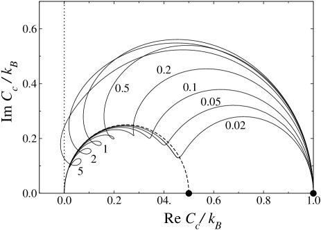
Figure 1: Imaginary versus real part of the complex heat capacity (47) for $\omega_{\ell}^{2}/\gamma^{2}=0$ (dashed line) and other values indicated (solid lines). The thermodynamic equilibrium, $\omega=0$, is indicated by a full circle. The vertical dotted line indicates the zero value of the real part.

To solve these equations we use a unitary transformation that diagonalizes the matrix $K$, transforming it in a diagonal matrix consisting of the eigenvalues $m\omega_{\ell}^{2}$ of $K$. By inspection of the equations it is seen that the matrices $A$, $B$ and $C$ become also diagonal. Denoting the diagonal elements denoted by $a_{\ell}$, $b_{\ell}$ and $c_{\ell}$, the equations for these variables are

$$(-i\omega+2\gamma)a_{\ell} = -2\omega_{\ell}^{2}c_{\ell}+\frac{2\gamma k_{\mbox{\tiny B}}T_{0}}{m},$$ (43)

$$-i\omega b_{\ell} = 2c_{\ell},$$ (44)

$$(-i\omega+\gamma)c_{\ell} = a_{\ell}-\omega_{\ell}^{2}b_{\ell}.$$ (45)

The quantity $\phi$, given by (24), and connected to the complex heat capacity by $C_{c}=\phi/i\omega T_{0}$, becomes $\phi=\gamma{\rm Tr}(A-k_{\mbox{\tiny B}}T_{0}I)$. Considering that the trace is invariant under a unitary transformation we find $\phi=\sum_{\ell}\phi_{\ell}$, where $\phi_{\ell}=\gamma(a_{\ell}-k_{\mbox{\tiny B}}T_{0})$. Solving the above equations for $a_{\ell}$, $b_{\ell}$ and $c_{\ell}$, we determine $\phi_{\ell}$ and

$$\phi=k_{\mbox{\tiny B}}T_{0}\sum_{\ell}\frac{i\omega\gamma}{\gamma-i\omega}\,\frac{\omega^{2}-4\omega_{\ell}^{2}+i\omega\gamma}{\omega^{2}-4\omega_{\ell}^{2}+2i\omega\gamma},$$ (46)

and reach the following result for the complex heat capacity

$$C_{c}=k_{\mbox{\tiny B}}\sum_{\ell}\frac{\gamma(\omega^{2}-4\omega_{\ell}^{2}+i\omega\gamma)}{(\gamma-i\omega)(\omega^{2}-4\omega_{\ell}^{2}+2i\omega\gamma)}.$$ (47)

The imaginary part versus the real part of $C_{c}$ is shown in figure 1. Notice that the real part, which is identified as the dynamical heat capacity, may be negative as seen in one of the curves of this figure.

Each term of the complex heat capacity $C_{c}$ has three poles, all located in the lower half-plane of the complex $\omega$, as shown in figure 2. If $4\omega_{\ell}^{2}>\gamma^{2}$, the poles are

$$\omega=\left\{\begin{array}[]{l}-i\gamma\\ -i\gamma\pm\sqrt{4\omega_{\ell}^{2}-\gamma^{2}}\end{array}\right.$$ (48)

If $4\omega_{\ell}^{2}<\gamma^{2}$, the poles are pure imaginary and given by

$$\omega=\left\{\begin{array}[]{l}-i\gamma\\ -i\gamma\pm i\sqrt{\gamma^{2}-4\omega_{\ell}^{2}}\end{array}\right.$$ (49)

The complex heat capacity (47) is thus analytic in the upper half-plane and vanishes as $1/|\omega|$ so that it obeys theKramers-Kronig relations.

Figure 2: (a) and (c) show the poles $\omega$ of the complex heat capacity $C_{c}$; and (b) and (d) show the eigenvalues $\Lambda$ of the unperturbed evolution operator ${\cal F}$. They are related by $\omega=i\Lambda$, that is, the poles are obtained from the eigenvalues through an anticlockwise rotation of $\pi/2$.

The real part of $C_{c}$ gives the time average of the dynamic heat capacity,

$$\overline{C}=k_{\mbox{\tiny B}}\sum_{\ell}\frac{2\gamma^{2}(\omega^{4}-6\omega_{\ell}^{2}\omega^{2}+8\omega_{\ell}^{4}+\gamma^{2}\omega^{2})}{(\omega^{2}+\gamma^{2})(\omega^{4}-8\omega_{\ell}^{2}\omega^{2}+16\omega_{\ell}^{4}+4\gamma^{2}\omega^{2})},$$ (50)

and its imaginary part gives the time average of the rate of entropy production,

$$\overline{\Pi}=k_{\mbox{\tiny B}}\sum_{\ell}\frac{\lambda\gamma\omega^{2}(\omega^{4}-8\omega_{\ell}^{2}\omega^{2}+16\omega_{\ell}^{4}+4\omega_{\ell}^{2}\gamma^{2}+\gamma^{2}\omega^{2})}{(\omega^{2}+\gamma^{2})(\omega^{4}-8\omega_{\ell}^{2}\omega^{2}+16\omega_{\ell}^{4}+4\gamma^{2}\omega^{2})}.$$ (51)

The rate of production of entropy $\overline{\Pi}$ is positive as demanded by expression (10). It vanishes when $\omega=0$ and reaches the value $\lambda\gamma nk_{\mbox{\tiny B}}$ when $\omega\to\infty$. The dynamic heat capacity vanishes in this limit. When $\omega=0$ it yields the value $nk_{\mbox{\tiny B}}$, which is the classical heat capacity of a harmonic solid with $n$ degrees of freedom.

The eigenvalues of the operator ${\cal F}$ is obtained by solving the eigenvalue equation ${\cal F}\psi=\Lambda\psi$. They can be found by assume a solution of the type $\psi=P_{0}G$ where $G(x,v)$ is the quadratic form

$$G=G_{0}+\frac{1}{2}\sum_{ij}(A_{ij}v_{i}v_{j}+B_{ij}x_{i}x_{j}+C_{ij}x_{i}v_{i}).$$ (52)

The replacement of this form into the eigenvalue equation, yields a set of equations for $A$, $B$ and $C$ which is found to be that given by equations (40), (41), and (42), with $-i\omega$ replaced by $\lambda$ and without the last term of (40). Proceeding in a similar manner, we find the eigenvalues of ${\cal F}$, which are shown in figure 2. If $4\omega_{\ell}^{2}>\gamma^{2}$, the eigenvalues are

$$\Lambda=\left\{\begin{array}[]{l}-\gamma\\ -\gamma\mp i\sqrt{4\omega_{\ell}^{2}-\gamma^{2}}\end{array}\right.$$ (53)

If $4\omega_{\ell}^{2}<\gamma^{2}$, the eigenvaues are real and given by

$$\Lambda=\left\{\begin{array}[]{l}-\gamma\\ -\gamma\pm\sqrt{\gamma^{2}-4\omega_{\ell}^{2}}\end{array}\right.$$ (54)

This confirms the result that the poles of the complex heat capacity are indeed given by $\omega=i\Lambda$.

5 Conclusion

Systems subject to a sinusoidal time dependent temperature are in a state of non-equilibrium and permanent production of entropy. In such a situation it is appropriate to analyzed them under the light of stochastic non-equilibrium thermodynamics. In theoretical studies of thermal modulation, the sinusoidal behavior of the heat flux is usually taken from granted. Using stochastic thermodynamics, we have demonstrated that this assumption is generally valid as long as the amplitude of the oscillations of temperature is small. That is, the heat flux behaves sinusoidally in time as the temperature but with a phase shift. If the amplitude is not small, the heat flux is still a periodic function of time but is not pure sinusoidal. Anyhow, the smallness of the amplitude of the temperature modulation is always met in experimental investigations so that we do not need to go beyond the linear approximation. In the case of harmonic forces, on the other hand, we have shown that it is not necessary to assume that the amplitude is small. In this case the heat flux will be always sinusoidal if the temperature is sinusoidal.

The pure sinusoidal behavior of the heat flux allowed the definition of the complex heat capacity whose real part is the dynamical heat capacity. The imaginary part of the complex heat capacity is interpreted as related to the net entropy flux in a cycle which equals the net production of entropy in a cycle. Here we have demonstrated this significant result achieved by Birge and Nagel [13] in their experimental investigations on the specific-heat spectroscopy. Our procedure is distinct from other approaches and is accurate enough to reach a precise relation between the imaginary part of the complex heat capacity and the entropy production, including the correct prefactor.

We have found and demonstrated a connection between the poles of the complex heat capacity and the eigenvalues of the unperturbed evolution operator. The former being the latter multiplied by the imaginary unit. In addition, we have shown that all poles are located in the lower half-plane of the complex frequency plane. The absence of poles in the upper half-plane implies the analyticity of the complex heat capacity in this region which in turn leads to the Kramers-Kronig relations. These results constitute some of the main results of the present study.

When the forces are harmonic, it is possible to solve exactly the FPK equation for any amplitude of the sinusoidal temperature. That is, it is possible to solve the FPK equation for any value of $\varepsilon$, not necessarily small. This is possible because in this case the time dependent probability distribution is Gaussian so that the only correlations that are needed are the pair correlations. We have carried out an exact calculations of the pair correlations from which we find exactly the complex heat capacity as a function of the frequency and obtained the frequency dispersion of the dynamic heat capacity and of the rate of entropy production.

It should be mentioned finally that all results obtained here, which include in the first place the possibility of the definition of a complex heat capacity, are founded on the sinusoidal behavior of the flux of heat. As we have demonstrated, this happens when the amplitude of the time oscillations of the temperature is small. It also happens when forces are harmonic, in which case the amplitude of temperature oscillations do not have to be small.

References

References

- [1] E. Gmelin, Thermochimica Acta 304/305, 1-26 (1997).
- [2] Y. Kraftmakher, Modulation Calorimetry, Theory and Applications (Springer, Berlin, 2004).
- [3] A. G. Worthing, Phys. Rev. 12, 199-225 (1918)
- [4] P. F. Gaehr, Phys. Rev. 12, 396-423 (1918).
- [5] K. K. Smith and P. W. Bigler, Phys. Rev. 19, 268-270 (1922).
- [6] L. I. Bockstahler, Phys. Rev. 25, 677-685 (1925).
- [7] C. Zwikker, Z. Physik 52, 668-677 (1925).
- [8] L. P. Filippov, Int. J. Heat Mass Transfer. 9, 681-691 (1966).
- [9] P. F. Sullivan and G. Seidel, Phys. Rev. 173, 679-685 (1968).
- [10] P. S. Gill, S. R. Sauerbrunn and M. Reading, Journal of Thermal Analysis 40, 931-939 (1993).
- [11] G. W. H. Höhne, W. F. Hemminger, and H.-J. Flammersheim, Differential Scanning Calorimetry (Springer, Berlin, 2003).
- [12] H. Gobrecht, K. Hamann and G. Willers, J. Phys. E: Sci. Instrum. 4, 21 (1971).
- [13] N. O. Birge and S. R. Nagel, Phys. Rev. Lett. 54, 2674 (1985).
- [14] Y.-H. Jeong, Thermochimica Acta 304/305, 67 (1997).
- [15] J. E. K. Schawe, Thermochimica Acta 304/305, 119 (1997).
- [16] G. W. H. Höhne, Thermochimica Acta 304/305, 121 (1997).
- [17] S. L. Simon and G. B. McKenna, J. Chem. Phys. 107 8678 (1997).
- [18] K. J. Jones, I. Kinshott, M. Reading, A. A. Lacey, C. Nikolopoulos, and H. M. Pollock, Thermochimica Acta 304/305, 187 (1997).
- [19] H. Baur and B. Wunderlich, Journal of Thermal Analysis 54, 437 (1998).
- [20] P. Claudy and J. M. Vignon, Journal of Thermal Analysis and Calorimetry 60, 333 (2000).
- [21] J.-L. Garden and J. Richard, Thermochimica Acta 461, 57 (2007).
- [22] T. Tomé, Braz. J. Phys. 36, 1285 (2006).
- [23] T. Tomé and M. J. de Oliveira, Phys. Rev. E 82, 021120 (2010).
- [24] C. Van de Broeck and M. Esposito, Phys. Rev. E 82, 011144 (2010).
- [25] R. E. Spinney and I. J. Ford, Phys. Rev. E 85, 051113 (2012).
- [26] F. Zhang, L. Xu, K. Zhang, E. Wang and J. Wang, J. Chem. Phys. 137, 065102(2012).
- [27] U. Seifert, Rep. Prog. Phys. 75, 126001 (2012).
- [28] M. Santillan and H. Qian, Physica A 392, 123 (2013).
- [29] D. Luposchainsky and H. Hinrichsen, J. Stat. Phys. 153, 828 (2013).
- [30] W. Wu and J. Wang, J. Chem. Phys. 141, 105104 (2014).
- [31] T. Tomé and M. J. de Oliveira, Phys. Rev. E 91, 042140 (2015).
- [32] T. Tomé and M. J. de Oliveira, Stochastic Dynamics and Irreversibility (Springer, Cham, 2015).
- [33] L. D. Landau and E. M. Lifshitz, Statistical Physics (Pergamon, London, 1958).
- [34] S. R. de Groot and P. Mazur, Non-Equilibrium Thermodynamics (North-Holland, Amsterdam, 1962).