Extended Scale-Free Networks

Résumé

Recently, Broido & Clauset (2019) mentioned that (strict) Scale-Free networks were rare, in real life. This might be related to the statement of Stumpf, Wiuf & May (2005), that sub-networks of scale-free networks are not scale-free. In the later, those sub-networks are asymptotically scale-free, but one should not forget about second-order deviation (possibly also third order actually). In this article, we introduce a concept of extended scale-free network, inspired by the extended Pareto distribution, that actually is maybe more realistic to describe real network than the strict scale free property. This property is consistent with Stumpf, Wiuf & May (2005) : sub-network of scale-free larger networks are not strictly scale-free, but extended scale-free.

1 From Strict Scale-Free to Scale-Free Types

scale-free network is a network whose degree distribution follows a power law, at least asymptotically. When studying internet networks, Barabási & Albert (1999) observed that some nodes, that they called hubs, had much more connections than others, and that the distribution of the number of links connecting to a node was a power-law. They coined the term scale-free network to describe that class of networks, when degrees have a power-law distribution. Clauset, Cosma & Newman (2007) studied real networks, and found some exhibiting that property. Nevertheless, recently, Broido & Clauset (2019) claimed that (strict) scale-free network are actually rare. More specifically, inspired by Alderson et al. (2009), they define various notions of weak or strong scale-free networks. If their taxonomy of scale-free network, in interesting we will consider here only the concept of strict scale-free if the degree distribution above a given cutoff $k_{\min}$ is a power law (as in Barabási & Albert (1999)).

As discussed in Voitalov et al. (2018), the scale-free property is closely related to the Pareto distribution, used in extreme value theory (and is the continuous version of the discrete power-law used for degrees). Nevertheless, as we will recall, this (strict) Pareto appears usually only above a very high threshold, and distributions are only Pareto type. Recently, Beirlant, Joossens & Segers (2009) suggested to take into account the second order approximation: the first order has a power law, and so is the second order, with smaller tail index. This is the extended Pareto distribution. In this article, we will explore an “extended scale-free” property, and study its impact on networks. And as we will see, this property is close to one described in Stumpf, Wiuf & May (2005) when studying sub-networks of larger ones.

1.1 Strict Scale-Free

Consider a network $(\mathcal{V},\mathcal{E})$, and let $n$ denote the number of nodes. Following Barabási & Albert (1999), the network is said to be scale-free if

$$p_{k_{\min}}(k)=\mathbb{P}[D=k]=Ck^{-\alpha},\leavevmode\nobreak\ \alpha>1,\text{ for }k\geq k_{\min}\geq 1$$

where $\alpha$ is the scaling exponent, and $C$ is the normalization constant. Inference is performed using a degree sequence $d_{1},\cdots,d_{n}$. Equivalently, the log-log plot should be linear (and the absolute value of the slope is the scaling exponent)

$$\log p_{k_{\min}}(k)=\log c-\alpha\log k.$$

This linear property for the logarithm of the frequency is the one usually used in network studies. Note that $p_{1}$ is also called Zipf’s distribution.

Definition 1.

The discrete Zipf’s distribution is defined as

$$p_{d-\text{Z},\alpha}(k)=\frac{1}{\zeta(\alpha)}k^{-\alpha}\text{ for }k\in\mathbb{N}_{+}=\{1,2,\ldots\}$$

where $\zeta()$ is Rieman’s function, $\displaystyle{\zeta(\alpha)=\sum_{k=1}^{\infty}k^{-\alpha}}$, defined for $\alpha>1$.

In this article, we exclude nodes that have $0$ connection. In many applications, some nodes are just disconnected from the others, having a null degree. In social networks, those individuals might be simple observers, and do not interact with others. This will also appear when considering sub-networks. Hence, when dealing with sub-networks in the last section of this article, we will remove nodes that are not connected to anyone.

1.2 Discrete PD with Cumulative Probabilities

Another popular approach is to consider cumulative probabilities, instead of frequencies. An interesting feature is that the cumulative probability of a power law probability distribution is also power law, but with an exponent $\alpha-1$. More specifically, let $\overline{F}(k)=\mathbb{P}[D>k]=1-\mathbb{P}[D\leq k]$ denote the complementary cumulative distribution function. If we consider a continuous version of $p(x)=Cx^{-\alpha}$, we obtain

$$\overline{F}(x)=\int_{x}^{\infty}p(t)dt=C\int_{x}^{\infty}t^{-\alpha}dt=\frac{Cx^{\alpha-1}}{\alpha-1}=\gamma x^{\alpha-1}$$

which is also a power function. And it is actually possible to derive a discrete probability function from a power $\overline{F}$ function, or more such as the (standard) Pareto function (see Arnold (1983) or chapter 20 in Johnson, Kotz & Balakrishnan (1994))

$$\overline{F}_{\text{PD},\xi}(x)=x^{-1/\xi}\text{ for }x\geq 1,$$

with $\xi>0$.

Definition 2.

The discrete strict Pareto distribution is defined as

$$p_{d-\text{PD},\xi}(k)=k^{-1/\xi}-(k+1)^{-1/\xi}\text{ for }k\in\mathbb{N}_{+}$$

defined for $\xi\in\mathbb{R}_{+}$.

For discretized version of continuous ones, we will use tail index $\xi$, having in mind the fact that $\alpha$ is of order $1+1/\xi$. The popular case $\alpha\in(2,3)$ means that $\xi\in(1/2,1)$, with $\alpha$ all the more small that $\xi$ is large. Observe that if the degrees have a discrete strict Pareto distribution, their expected value is

$$<D_{d-\text{P}}>=\sum_{k=1}^{\infty}kp_{d-\text{PD},\xi}(k)=\sum_{k=1}^{\infty}k^{-1/\xi}=\zeta(1/\xi)$$

which is different from $(1-\xi)^{-1}$ obtained with a continuous Pareto distribution.

1.3 Discrete GPD and Second Law of Extremes

Pareto distributions are very popular since the second law of extremes (see Pickands (1975) and Balkema & de Haan (1974)) which states that if $X$ is a random variable such that there exists a function $a(u)$ such that

$$a(u)^{-1}(X-u)|X>u\rightarrow Z,\text{ as }u\rightarrow\infty$$

(in the weak convergence sense) for some non-degenerate $Z$ on $\mathbb{R}_{+}$, then $Z$ follows a Generalized Pareto (GPD) with complementary cumulative distribution function

$$\overline{F}_{\text{GPD},\sigma,\xi}(x)=\mathbb{P}[Z>x]=\left(1+\xi\frac{x}{\sigma}\right)^{-1/\xi},\text{ for }x\geq 0.$$

As a consequence, for large $u$, we have usually the approximation for $\mathbb{P}[X-u>x|X>u]$

$$\mathbb{P}[a(u)\big{(}a(u)^{-1}(X-u)\big{)}>x|X>u]\sim\mathbb{P}[a(u)Z>x]=\mathbb{P}[Z>a(u)^{-1}x]=\overline{F}_{\text{GPD},\sigma a(u),\xi}(x)$$

as suggested in Davison & Smith (1990). We will then write $X\in\text{MDA}_{\xi}$ - for Max-Domain of Attraction. Nevertheless, as proved in Anderson (1980) and Shimura (2012), this approximation might not be valid if $X$ as a discrete support. An important additional property if to have a long-tailed distribution for $\overline{F}$ in the sens that

$$\frac{\overline{F}(u+1)}{\overline{F}(u)}\rightarrow 1\text{ as }u\rightarrow\infty$$

As proved in Shimura (2012), a discrete random variable $X\in\text{MDA}_{\xi}$ if and only if (i) $\overline{p}$ is long-tailed and (ii) $X=\lceil X^{\star}\rceil$ where $X^{\star}\in\text{MDA}_{\xi}$. And in that case,

$$p_{u}(u+k)=\mathbb{P}[X-u=k|X>u]\approx p_{d-\text{GPD},a(u)\sigma,\xi}(k),\text{ for }k\in\mathbb{N}$$

Thus, following Krishna & Pundir (2009), define :

Definition 3.

The discrete generalized Pareto distribution is defined as

$$p_{d-\text{GPD},\sigma,\xi}(k)=\overline{F}_{\text{GPD},\sigma,\xi}(k-1)-\overline{F}_{\text{GPD},\sigma,\xi}(k)=\left(1+\xi\frac{k-1}{\sigma}\right)^{-1/\xi}-\left(1+\xi\frac{k}{\sigma}\right)^{-1/\xi}\text{ for }k\in\mathbb{N}_{+}$$

defined for $\xi\in\mathbb{R}_{+}$.

A (continuous) GPD random variable can be expressed as a mixture of exponential variables, that is an exponential random variable with a Gamma distributed rate parameter : if $X^{\star}\sim\mathcal{E}(\Lambda)$ with $\Lambda\sim\mathcal{G}(\alpha,\beta)$, then $X^{\star}$ has a GPD distribution, with tail index $\xi=1/\alpha$. Interestingly, as proved in Buddana & Kozubowski (2014), a similar property holds for the discrete $d$-GPD, which is a mixture of geometric variables (with also Gamma heterogeneity).

The three probability distributions ($p_{d-\text{Z}}$, $p_{d-\text{P}}$ and $p_{d-\text{GPD}}$), for similar tail exponent $\xi$, can be visualized on Figure 1 (for the Zipf, $\alpha=1+1/\xi$).

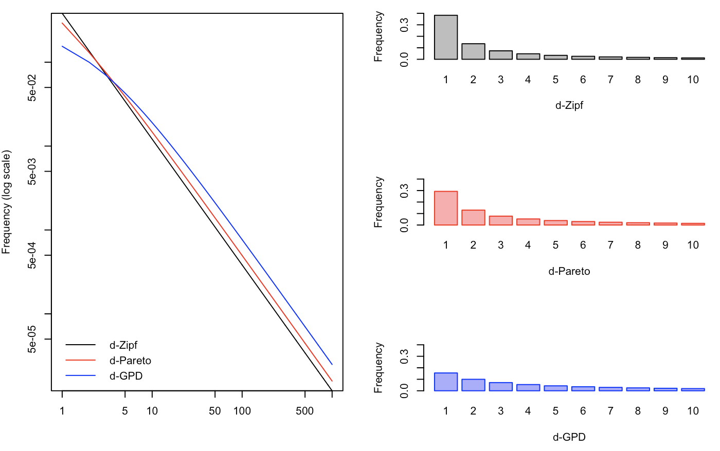
Figure 1: $p_{d-\text{Z}}$, $p_{d-\text{P}}$ and $p_{d-\text{GPD}}$, on a log-log scale on the left, and for the first 10 values on the right, with the same index $\xi$.

1.4 Regular Variation and Power-Law Type

This power law property is deeply related to the concept of scale-free distribution : scale-free means that the distribution is the same whatever scale we consider. Hence, for any $\lambda$, $f(\lambda k)$ is proportional to $f(k)$, or $f(\lambda k)=h_{\lambda}f(x)$ (we must consider here the continuous version $f$ and not $p$ since, unless $\lambda\in\mathbb{N}$, $\lambda k$ is not always an integer). Thus, since $h_{\lambda}=f(\lambda)/f(1)$, we get that $f(\lambda x)=f(\lambda)\cdot f(x)$, which is the multiplicative version of Cauchy’s functional equation (also called Hamel-Cauchy), with unique solution $f(x)=x^{-\alpha}$ (up to a multiplicative constant). Hence, scale-free means that $f(\lambda x)/f(x)$ is constant (and in that case, $f(x)=Cx^{-\alpha}$). A natural extension is to assume that $f(\lambda x)/f(x)$ is asymptotically constant.

A function $g$ is said to be regularly varying (at infinity) if $g(tx)/g(x)$ tends to $t^{\theta}$, for some $\theta\in\mathbb{R}$, when $t$ goes to infinity. If $\theta=0$, then $g$ is said to be slowly varying, to derive an extended version of the power law.

Definition 4.

A continuous variable $X^{\star}$ is said to be Pareto-type distributed, with tail exponent $\xi$ if $\mathbb{P}[X^{\star}>x]=x^{-1/\xi}\ell(x)$ for some slowly varying function $\ell$.

In section 2, the idea will be to consider a simple parametric expresion for function $\ell$, that will decay to a constant at some power speed.

1.5 Probability-Generating Function of Scale-Free Distribution

An alternative way to describe the distribution is not to use $p$, but its probability-generating function (PGF), $G(s)$, defined as

$$G(s)=\sum_{k=0}^{\infty}p(k)s^{k},$$

for instance, with a Poisson variable, ${\displaystyle G(z)=e^{\lambda(z-1)}}$, while with a power law, or a scale free distribution

$$G(s)=\frac{1}{\zeta(\alpha)}\sum_{i=1}^{\infty}i^{-\alpha}s^{i}=\frac{\text{Li}_{\alpha}(s)}{\zeta(\alpha)}$$

where $\text{Li}_{\alpha}$ is Jonquière’s polylogarithm function (see Abramowitz & Stegun (1972)). We will use that alternative representation when focusing on sub-networks.

2 Extended Scale-Free

The Extended Pareto Distribution (EPD) was introduced in Beirlant, Joossens & Segers (2009), and there are many way to derive that distribution, most of them being equivalent.

2.1 Mixture of Scale-Free

Hall (1982) suggested to write a Pareto type distribution $\overline{F}(x)=x^{-1/\xi}\ell(x)$ as $\overline{F}(x)=x^{-1/\xi}\cdot C(1-\delta(x))$. Here, $\ell$ is not only slowly varying, but also $\ell(x)$ tends to $C$ when $x$ goes to infinity (at some power rate). More specifically, assume that $\delta(x)=Dx^{\beta}+o(x^{\beta})$ where $\beta<0$. If $\delta(x)=Dx^{\beta}$, we can write

$$\overline{F}(x)=C_{1}x^{-\gamma_{1}}+C_{2}x^{-\gamma_{2}}$$

which can be seen as a mixture of two (strict) Pareto distributions.

2.2 Second-Order Regular Variation

The first law of extremes (also called Fisher-Tippett theorem) is based on the limiting distribution of maximum $x_{(n)}$ of an i.i.d. sample $\{x_{1},\cdots,x_{n}\}$. More precisely, assume that there exists a function $a(n)$ such that

$$a(n)^{-1}\big{[}X_{(n)}-F^{-1}(1-1/n)\big{]}\rightarrow Z,\text{ as }n\rightarrow\infty$$

for some non-degenerate $Z$ on $\mathbb{R}_{+}$, then $Z$ follows a Generalized Extreme Value (GEV) distribution (see Embrechts, Klüppelberg & Mikosch (1997) or Beirlant et al. (2004)). Let $U$ denote the quantile function $U(x)=F^{-1}(1-1/x)$, then somehow, we might be interested by the limit (if it exists) of $a(n)^{-1}(U(xn)-U(n))$ when $n$ goes to infinity. This is related to the concept of extended regular variation (see de Haan & Ferreira (2006)) : $g$ is said to be $ERV_{\gamma}$ if

$$\lim_{t\rightarrow\infty}\frac{g(tx)-g(t)}{a(t)}=c\frac{x^{\gamma}-1}{\gamma}$$

which can be seen as extension of regular variation of index $\gamma$. For instance, the quantile function of a (strict) Pareto distribution with index $\xi$, $U(x)=x^{\xi}$, and with auxiliary function $a(t)=\xi t^{\xi}$, $a(n)^{-1}(U(xn)-U(n))=(x^{\xi}-1)/\xi$ (see Beirlant et al. (2004)).

Second order regular variation is obtained assuming that there is a function $b$ such that

$$\lim_{t\rightarrow\infty}\frac{1}{b(t)}\left[\frac{g(tx)-g(t)}{a(t)}-\frac{x^{\gamma}-1}{\gamma}\right]$$

exists, and is denoted $h(x)$. de Haan & Stadtmüller (1996) obtained a general expression for $h$, related to some index $\rho$. In a nutshell, following Drees (1998) and Cheng & Jiang (2001), the limit can be expressed

$$\lim_{t\rightarrow\infty}\frac{1}{b(t)}\left[\frac{g(tx)-g(t)}{a(t)}-\frac{x^{\gamma}-1}{\gamma}\right]=\frac{x^{\gamma+\rho}-1}{\gamma+\rho}$$

with $\rho<0$ (theorem B.3.10 in Albrecher, Beirlant & Teugels (2017)).

2.3 Extended Scale-Free

For the strict Pareto distribution, we have seen that

$$\lim_{t\rightarrow\infty}x^{-\gamma}\frac{\overline{F}(tx)}{\overline{F}(t)}=1$$

But let us consider the following extension (based on the expression of the second-order regular variation)

$$\lim_{t\rightarrow\infty}x^{-\gamma}\frac{\overline{F}(tx)}{\overline{F}(t)}=1+\frac{x^{\rho}-1}{\rho},\text{ for some }\rho\leq 0$$

or, up to some affine transformation, $\overline{F}(x)=cx^{-\gamma}[1+x^{\rho}\ell(x)]$. Since $(1+u)^{b}\sim(1+bu)$, define (changing $\gamma$ in $\alpha$, $\rho$ in $\tau$)

$$\overline{F}(x)=\mathbb{P}[X>x]={\left[x\left(1+\delta-\delta x^{\tau}\right)\right]^{-1/\xi}},\text{ for }x\geq u$$

where $\tau\leq 0$ and $\delta>\max(-1,1/\tau)$. This is the Extended Pareto Distribution, as define in Beirlant, Joossens & Segers (2009).

Definition 5.

The discrete extended Pareto distribution is defined as

$$p_{d-\text{EPD},\delta,\tau,\xi}(k)=\overline{F}_{\text{EPD},\delta,\tau,\xi}(k-1)-\overline{F}_{\text{EPD},\delta,\tau,\xi}(k)={\left[(k-1)\left(1+\delta-\delta\left(k-1\right)^{\tau}\right)\right]^{-1/\xi}}-{\left[k\left(1+\delta-\delta k^{\tau}\right)\right]^{-1/\xi}}\text{ for }k\in\mathbb{N}_{+}$$

Figure 2: $p_{d-\text{Z}}$ and $p_{d-\text{mix-P}}$ on a log-log scale on the left, and $p_{d-\text{Z}}$ and $p_{d-\text{EP}}$ on the right.

Figure 3: $\overline{F}_{d-\text{Z}}$ and $\overline{F}_{d-\text{mix-P}}$ on a log-log scale on the left, and $\overline{F}_{d-\text{Z}}$ and $\overline{F}_{d-\text{EP}}$ on the right.

2.4 Shifted Pareto Distributions

So far, we defined (discrete) distributions for degrees taking values in $\{1,2,3,\ldots\}$. Quite naturally, one can that $D$ has a Pareto distribution with a shift of $u\in\mathbb{N}_{+}$ if $D-u$ has a Pareto distribution. For instance, with a strict Pareto distribution, when plotting the complementary cumulative probability function $\overline{F}_{d-\text{PD}}$ on a log-log scale, the function is a (semi)-straight line with slope $-1/\xi$, starting in $(u,2^{-1/\xi})$.

3 Inference & Estimation of $\alpha$ or $\xi$

3.1 Inference for Continuous Pareto Distributions (Hill Estimator)

In order to estimate $\alpha$, or $1/\xi$, the power exponent, we can use classical estimators obtained on continuous observations. More specifically, for a strict Pareto sample, use Hill estimate, given a sample $\{x_{1},\cdots,x_{n}\}$, sorted, such that $x_{(1)}\leq x_{(2)}\leq\cdots\leq x_{(n)}$,

$$\widehat{\xi}=\frac{1}{n}\sum_{i=1}^{n}\log x_{(i)}-\log x_{(1)}$$

(see Appendix 6.1 for a brief justification) but one can also focus on the $k$ largest values

$$\widehat{\xi}_{k}=\frac{1}{k}\sum_{i=n-k+1}^{n}\log x_{(i)}-\log x_{(n-k)}$$

This estimator is strongly consistent, $\widehat{\xi}_{k}\overset{a.s.}{\rightarrow}\xi$ and (with further assumptions, see Embrechts, Klüppelberg & Mikosch (1997))

$$\sqrt{k}\big{(}\widehat{\xi}_{k}-\alpha\big{)}\overset{\mathcal{L}}{\rightarrow}\mathcal{N}(0,\xi^{2})$$

Nevertheless, this estimator performs badly when the sample is not strictly Pareto distributed, see Figure 4. For the EPD, Albrecher, Beirlant & Teugels (2017) suggest to use maximum likelihood techniques.

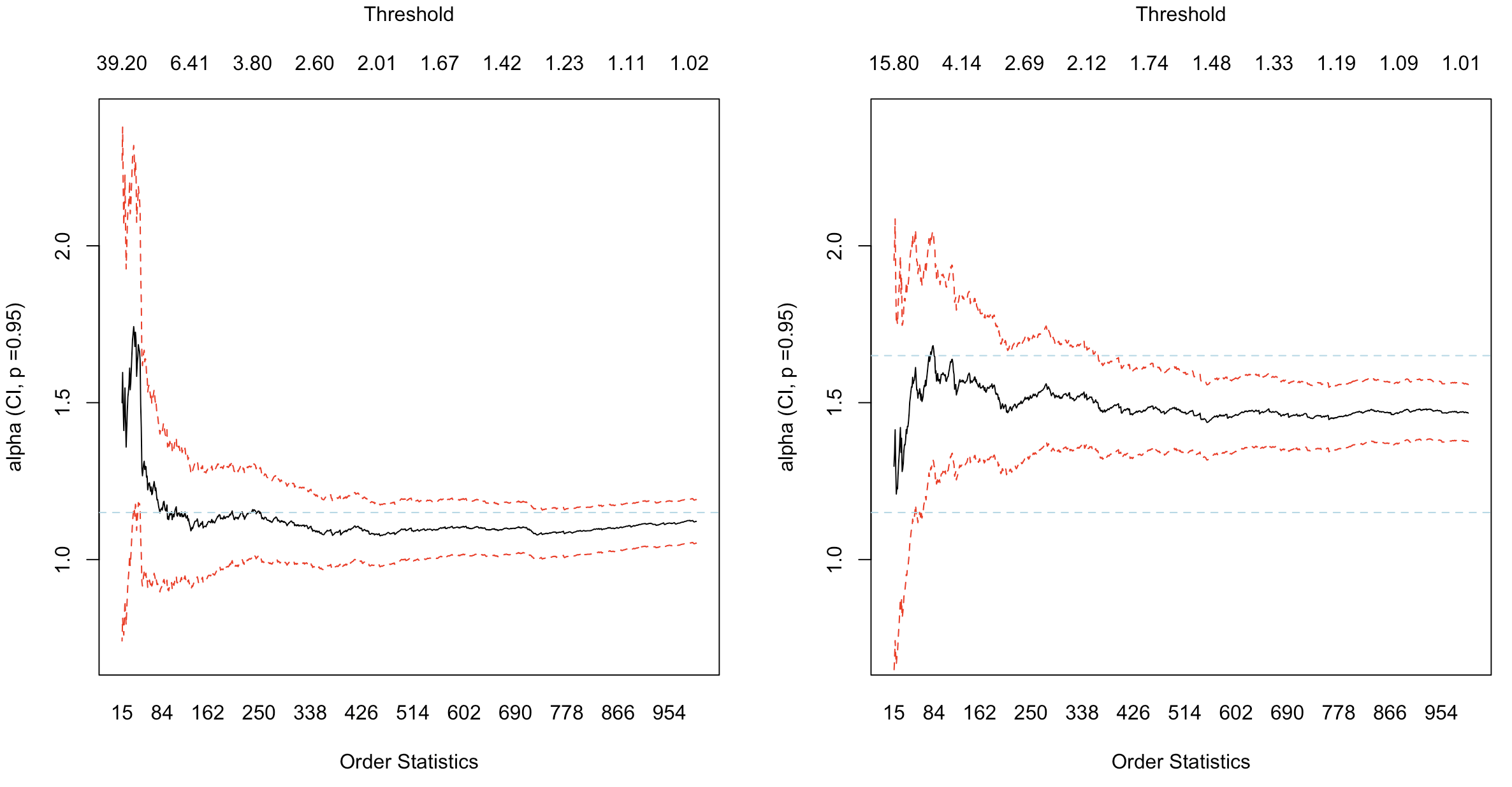
Figure 4: Hill plot, for a (strict) scale free distribution on the left, and an extended scale-free distribution on the right.

3.2 Inference for Discrete Pareto Distributions

Two techniques are used to estimate parameters (whatever the underlying scale-free distribution considered). The first one is based on the chi-square statistic,

$$Q(\boldsymbol{\theta})=\sum_{k=1}^{k_{\max}}\frac{(n\cdot p_{d-\star,\boldsymbol{\theta}}(k)-n_{k})^{2}}{n\cdot p_{d-\star,\boldsymbol{\theta}}(k)}$$

where $n_{k}$ is the number of nodes with exactly $k$ neighbors. Actually, to get a more robust version, if $n_{k}$ is too small, we will regroup per classes, to have (at least) 10 nodes per class (see Appendix 6.2). An alternative is to use maximum likelihood techniques (see Appendix 6.2).

4 Strict and Extended Scale-Free Networks

Before studying real networks, let us generate networks that are extended scale-free, to see what they look like.

4.1 Generating a Network from Degree Distribution

Consider a sequence $d_{1},\cdots,d_{n}$ of non-negative integers such that $d_{n}\leq\cdots\leq d_{1}$. From Erdös-Gallai theorem, see Tripathi, Venugopalan & West (2010), that sequence can be represented as the degree sequence of a finite simple graph on $n$ vertices if and only if $d_{1}+\cdots+d_{n}$ is even, and

$${\displaystyle\sum_{i=1}^{k}d_{i}\leq k(k-1)+\sum_{i=k+1}^{n}\min(d_{i},k)}$$

holds for every ${\displaystyle 1\leq k\leq n}$. In this section, we use the methodology described in Newman (2002) to generate graphs with an Extended Pareto distribution for the degree

4.2 Network Structures

On Figure 5, we can see the average shortest path for all nodes in the largest connected subgraph. This was obtained by averaging 1,000 simulated networks with $n=1,000$ nodes, with various $\tau$. The larger the absolute value of $\tau$, the longer the average shortest-path distance.

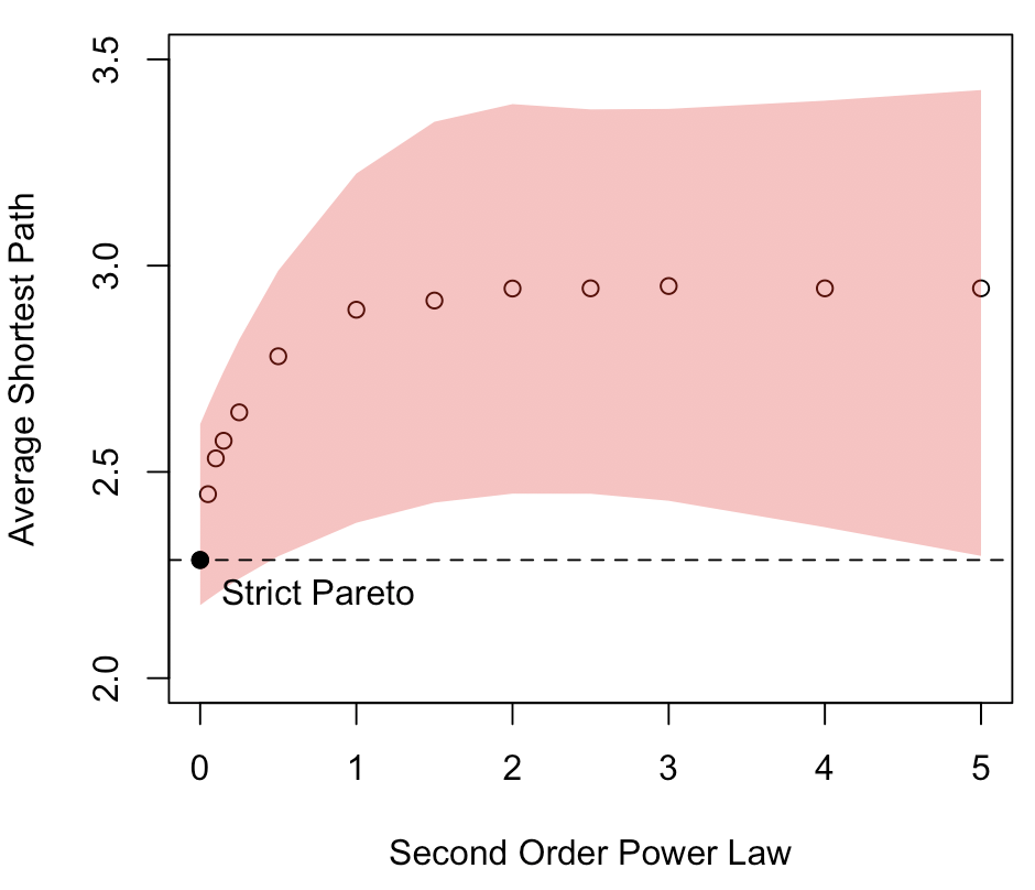
Figure 5: Average shortest path on simulated networks with $n=1,000$ notes, when degrees have an extended scale free distribution $EPD(\gamma=1.15,\kappa,\tau)$ when $-\tau$ varies from $0$ (strict Pareto) to $5$. The shaded area is the $90\%$ confidence band obtained with 500 simulated networks (for each $\tau$).

Heuristically, this can be explained since with a strict power law distribution, sub-graphs are connected to each other through (big) hubs, and those network have a small-world property : everyone is close to anyone. With a (strong) second order, there are less very big hubs, and more smaller one : the distance w to anyone tends to be, on average, longer.

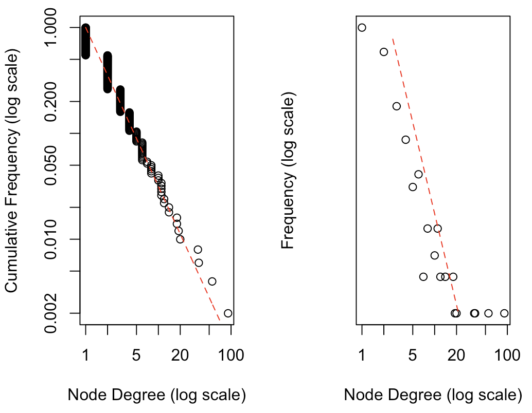
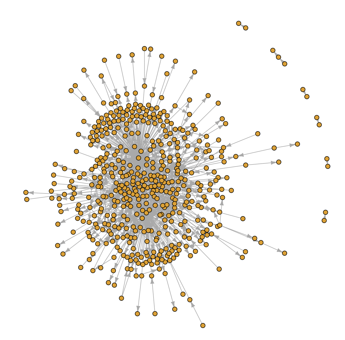
Figure 6: Strict Scale Free Network

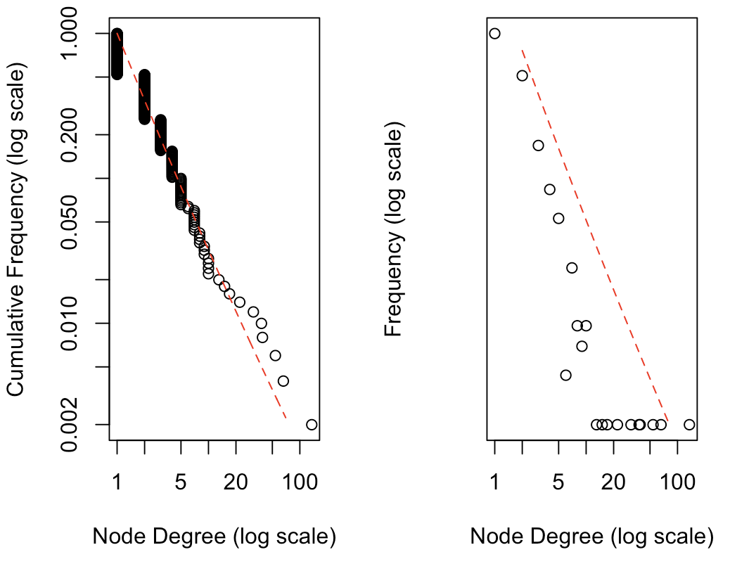
Figure 7: Extended Scale Free Network

4.3 Sub-network of Scale-Free Networks

Stumpf, Wiuf & May (2005) claimed that sub-networks of scale-free networks are not scale-free anymore. Of course, this result depend on how we sub-sample from a general network, and how scale-free is defined. Let $\{\mathcal{V},\mathcal{E}\}$ a network, i.e. a collection of vertices and edges. Let $A$ denote its adjacency matrix : let $i$ and $j$ denote two nodes in $\mathcal{V}$, then $A_{i,j}=1$ if an only if $(i-j)$ is in $\mathcal{E}$. We assume here that there are no zero-degree node, i.e. $\forall i\in\mathcal{V}$, $\exists j\in\mathcal{V}$ such that $A_{i,j}=1$.

To generate a sub-network, select randomly (and uniformly) a sub-sample of nodes $\mathcal{V}^{*}$, then extract the sub-adjacency matrix $A^{\star}$, and the $(i-j)$ is in $\mathcal{E}$ if an only if $A^{\star}_{i,j}=1$. Interestingly, one can easily write the PGF of the degree distribution on the sub-network,

$$G^{*}(s)=G(1-p(1-s))$$

where $p$ is the probability to keep a given node. Since we excluded orphaned nodes, it is necessary to rescale the PGM, and then

$$G^{*}(s)=\frac{G(1-p(1-s))}{1-G(1-p)}$$

As discussed in Stumpf, Wiuf & May (2005), if we get back to simple scale-free network, we can obtain the following

$$\mathbb{P}[d=k]\sim\frac{1}{k},\text{ then }\mathbb{P}[d>k]\sim\frac{1}{k^{2}}\text{ while }\mathbb{P}^{*}[d^{*}>k]\sim\frac{1}{k(k-1)}$$

$$\mathbb{P}[d=k]\sim\frac{1}{k^{2}},\text{ then }\mathbb{P}[d>k]\sim\frac{1}{k^{3}}\text{ while }\mathbb{P}^{*}[d^{*}>k]\sim\frac{1}{k(k-1)(k-2)}$$

Observe that those two reminds us of the Hall class (see Hall (1982)). Hence

$$\frac{1}{k(k-1)}=[k^{2}(1-k^{-1})]^{-1}$$

which is an extended Pareto distribution with index $\tau=-1$.

5 Real Internet Networks

In order to illustrate this second order property, we will use data from the Stanford Network Analysis Project (SNAP), from Facebook, Twitter and Google Plus (see McAuley & Leskovec (2012)). The first one contains 4,039 nodes and 88,234 edges, the second one contains 81,306 nodes and 1,768,149 edges and the third 107,614 nodes and 13,673,453 edges.

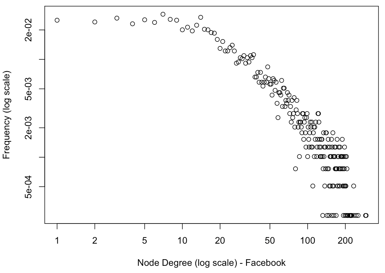
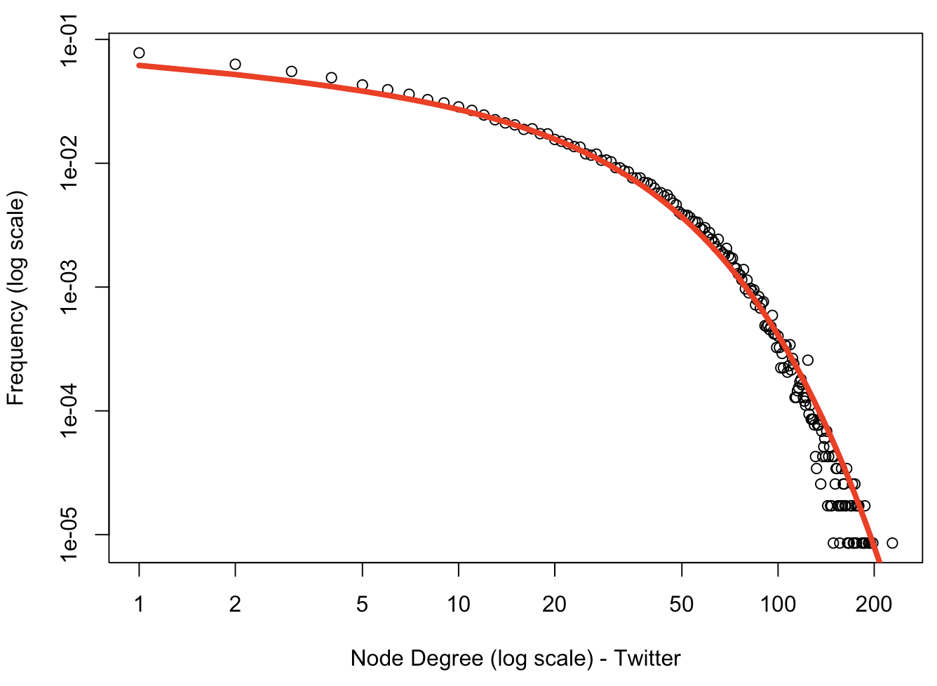
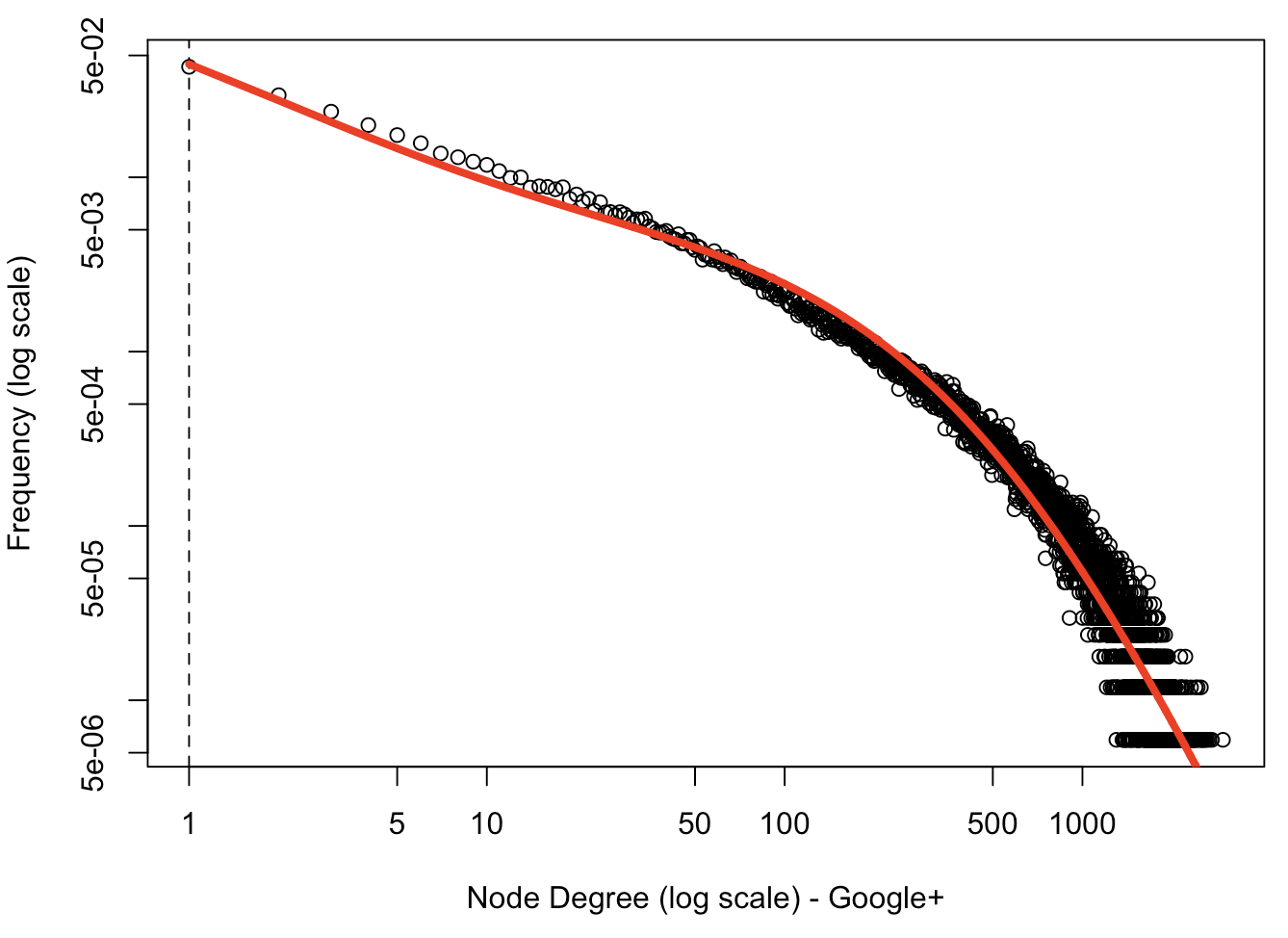
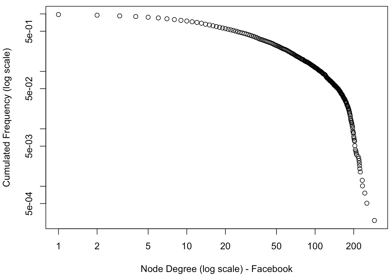
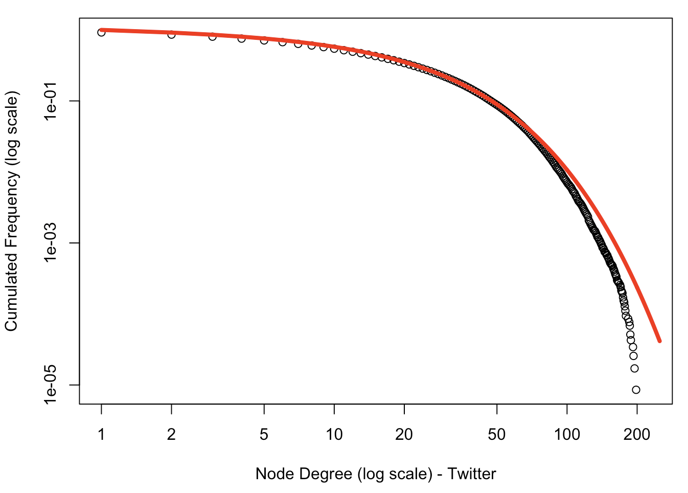
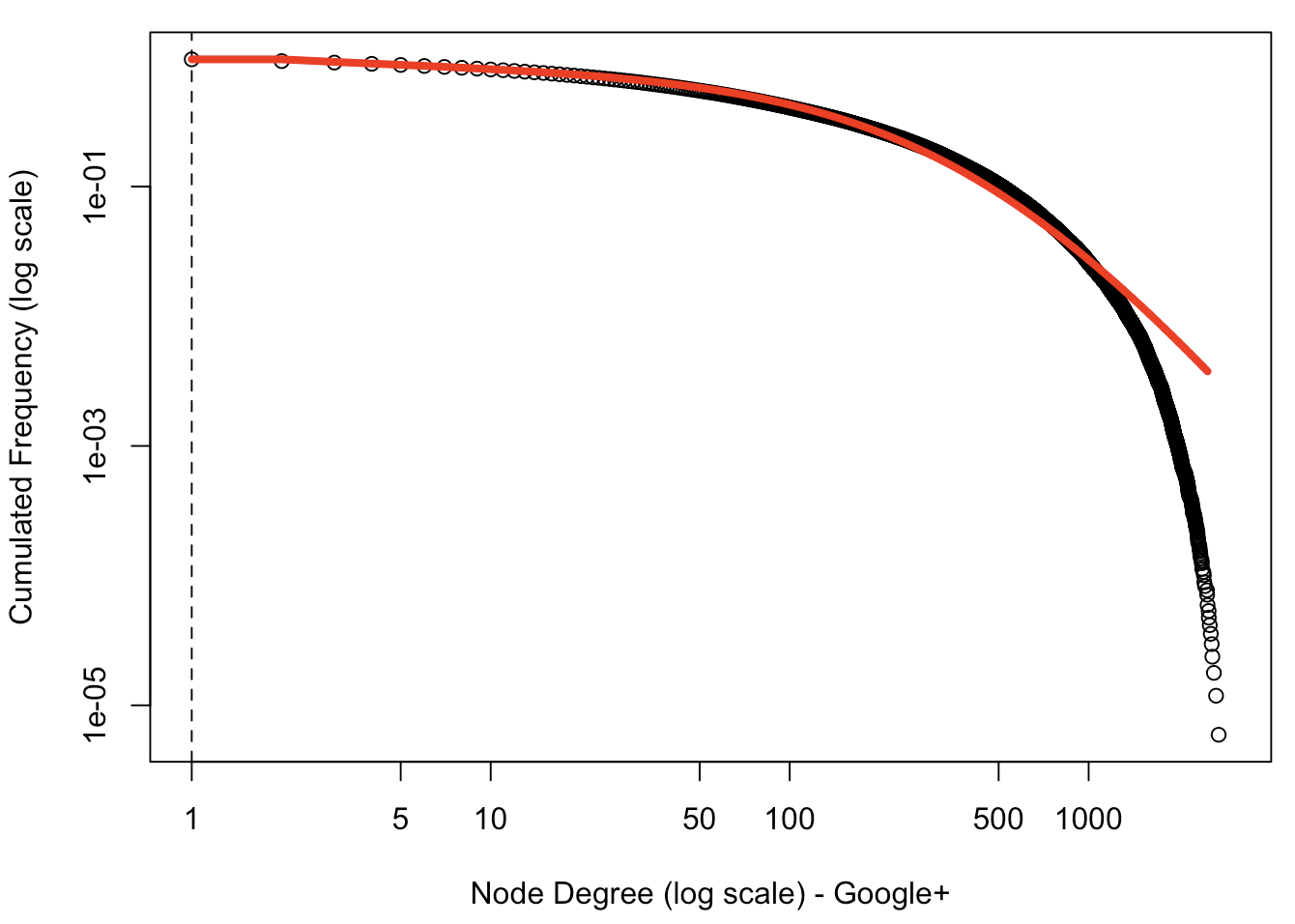
Figure 8: Distribution of degrees on Facebook sub-network (left), Twitter (center) and Googple+ (right), including the extended scale free distribution (estimated by maximum likelihood) for Twitter and Google+.

In the SNAP-Facebook dataset, we have we have 10 sub-networks. It is known for being a not scale-free network, see Gjokaf. This is confirmed on the left of Figure 8 where no extended distribution can be used to capture such a strong concavity.

For the Twitter network, Aparicio, Villazón-Terrazas & Álvarez (2015) fitted a scale free distribution $\mathbb{P}(k)\sim Ck^{-\lambda}$, outgoing degree distribution has tail index of $\widehat{\lambda}=2.1715$ while incoming degree distribution has tail index $\widehat{\lambda}=1.8778$. Here, we did not distinguish incoming and outgoing edges. When fitting an extended Pareto distribution, we obtained $\widehat{\xi}=0.757$ (or $1+\widehat{\xi}^{-1}=2.32$, consistent with the values obtained in Aparicio, Villazón-Terrazas & Álvarez (2015)) and $\widehat{\tau}=-1$. For Google+, we obtained also $\widehat{\tau}=-1$. This value is consistent with the result obtained in Stumpf, Wiuf & May (2005), and can be visualized on the center of Figure 8 (for Twitter network) and on the right of 8 (for Google+ network). On those two sets of figures, the parametric fitted distribution is added to the scatterplot.

6 Appendix

6.1 Fitting Continuous Distributions

Consider a continuous power law distribution, with density

$$f(x)=(\alpha-1)x^{-\alpha},\leavevmode\nobreak\ x\geq 1.$$

The likelihood of a sample $\boldsymbol{x}=\{x_{1},\ldots,x_{n}\}$ is then

$$\mathcal{L}(\alpha;\boldsymbol{x})=\prod_{i=1}^{n}f(x_{i})=\prod_{i=1}^{n}(\alpha-1)(x_{i})^{-\alpha}$$

For convenience, use the logarithm of the likelihood,

$$\log\mathcal{L}(\alpha;\boldsymbol{x})=\sum_{i=1}^{n}\log(\alpha-1)-\alpha\log(x_{i})$$

The maximum of the logarithm of the likelihood function is obtained when

$$\left.\frac{\partial\log\mathcal{L}(\alpha;\boldsymbol{x})}{\partial\alpha}\right|_{\alpha=\widehat{\alpha}}=0\text{ i.e. }\widehat{\alpha}=1+n\left(\sum_{i=1}^{n}\log(x_{i})\right)^{-1}$$

6.2 Fitting Discrete Distributions

It was mentioned in section 3.2 that the chi-square distance can be used to estimate the (unknown) parameter

$$Q(\boldsymbol{\theta})=\sum_{k=1}^{k_{\max}}\frac{(np_{d-\star,\boldsymbol{\theta}}(k)-n_{k})^{2}}{np_{d-\star,\boldsymbol{\theta}}(k)}$$

A more robust version can be obtained by regrouping too-small degrees, to have at least 10 nodes : consider some (consecutive) partition $\mathcal{K}_{1},\ldots,\mathcal{K}_{m}$ such that $\sum_{k\in\mathcal{K}_{j}}n_{k}\geq 10$ for all $j$, and then

$$Q(\boldsymbol{\theta})=\sum_{j=1}^{m}\frac{(np_{d-\star,\boldsymbol{\theta}}(\mathcal{K}_{j})-n_{\mathcal{K}_{j}})^{2}}{np_{d-\star,\boldsymbol{\theta}}(\mathcal{k}_{j})}$$

where

$$n_{\mathcal{K}_{j}}=\sum_{k\in\mathcal{K}_{j}}k\text{ and }p_{d-\star,\boldsymbol{\theta}}(\mathcal{K}_{j})=F_{\star}(\max\{\mathcal{K}_{j}\})-F_{\star}(\min\{\mathcal{K}_{j}\}-1)$$

Then the estimator is

$$\widehat{\boldsymbol{\theta}}=\text{argmin}\{Q(\boldsymbol{\theta})\}$$

For the discrete EPD model, given a vector x of degrees, the R code to compute the chi-square distance between the empirical distribution and $p_{d-\text{EPD}}$ is, for some given $\boldsymbol{\theta}$ (i.e. values gamma, tau and kappa)

    T = table(x)
    T2 = T[as.character(1:max(as.numeric(names(T))))]
    names(T2) = as.character(1:max(as.numeric(names(T))))
    T2[is.na(T2)] = 0
    k = 1
    sumt2 = 0
    VK = NULL
    k0 = k
    while(k<=max(as.numeric(names(T)))){
      sumt2=sumt2+T2[as.character(k)]
      if(sumt2<10){k=k+1}
      if(sumt2>=10){VK=rbind(VK,c(k0,k,sumt2))
      k0=k
      k=k+1
      sumt2=0}
    }
    VK[2:nrow(VK),1] = VK[2:nrow(VK),1]+1
    PEMP = VK[,3]/(VK[,2]+1-VK[,1])/sum(VK[,3])
    PEPD = pepd(VK[,2]+1,gamma=gamma,tau=tau,kappa=kappa)-
           pepd(VK[,1],gamma=gamma,tau=tau,kappa=kappa)
    VK = cbind(VK,PEMP,PEPD)
    Q = sum( (PEMP-PEPD)^2/PEPD )

Then we use an optimization route (mainly function optim()) to find $\widehat{\boldsymbol{\theta}}$.

The maximum likelihood is obtained here with a slight change at the end of the previous code

    PEPD=pepd(x+1,gamma=gm,tau=ta,kappa=kp)-
         pepd(x,gamma=gm,tau=ta,kappa=kp)
    MLE=-sum(log(PEPD))

Then, use optim to find the maximum of the log-likelihood, or the minimum of the chi-square distance.

On Figure 9, we can visualize the boxplots of the six-estimators of $\alpha$ considered here, on 1,000 simulated samples, with two techniques and three underlying distribution (a discrete strict Pareto with tail index $alpha=1.15$). On the left, we use the chi-square minimum distance, and on the right, the maximum-likelihood technique. We consider either a strict Pareto, a Generalized Pareto (GPD) and the Extended Pareto (EPD).

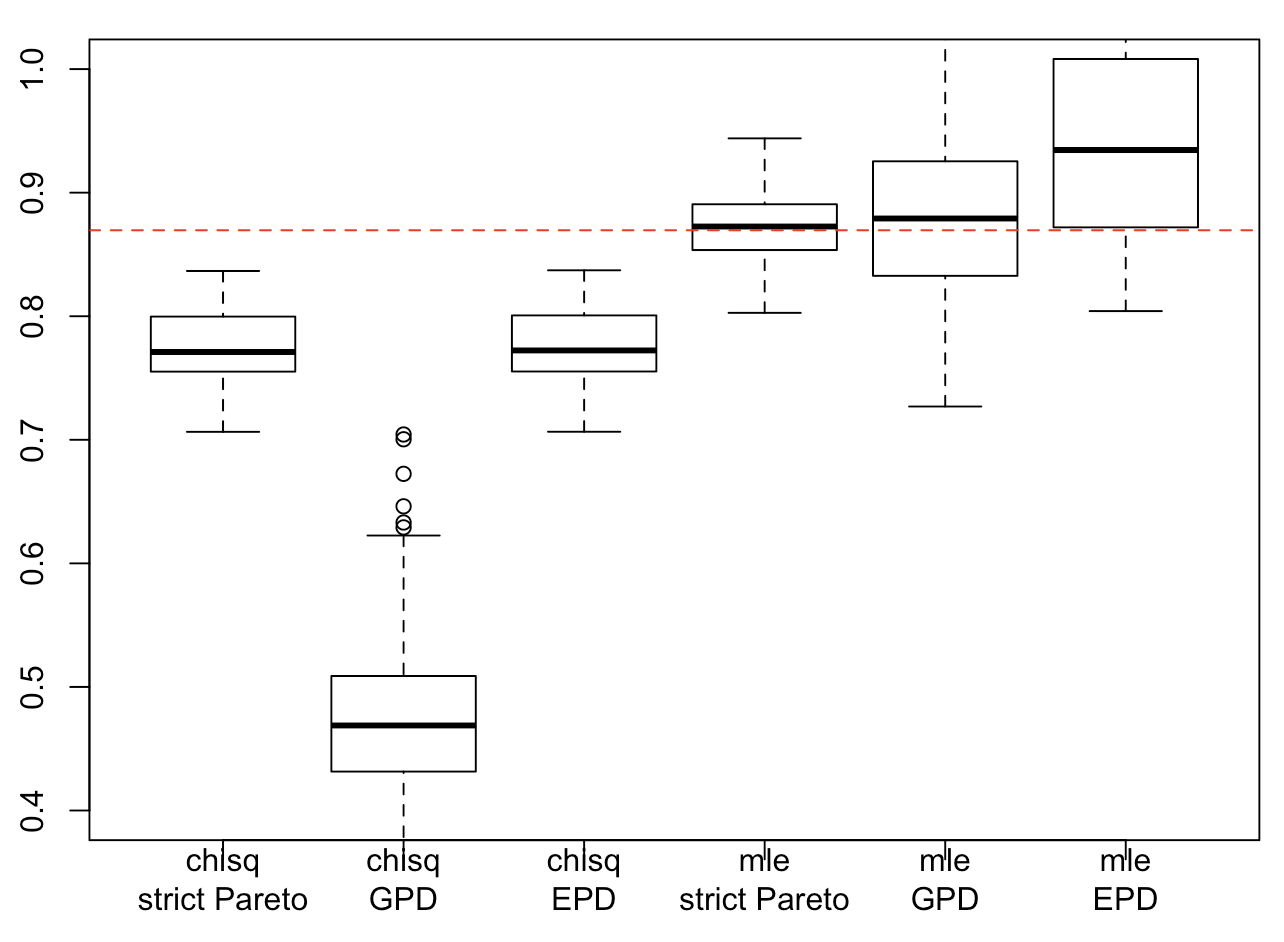
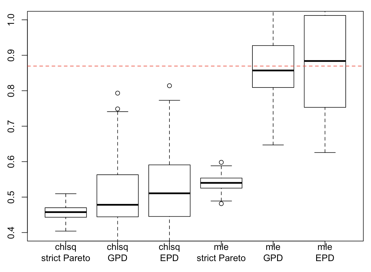
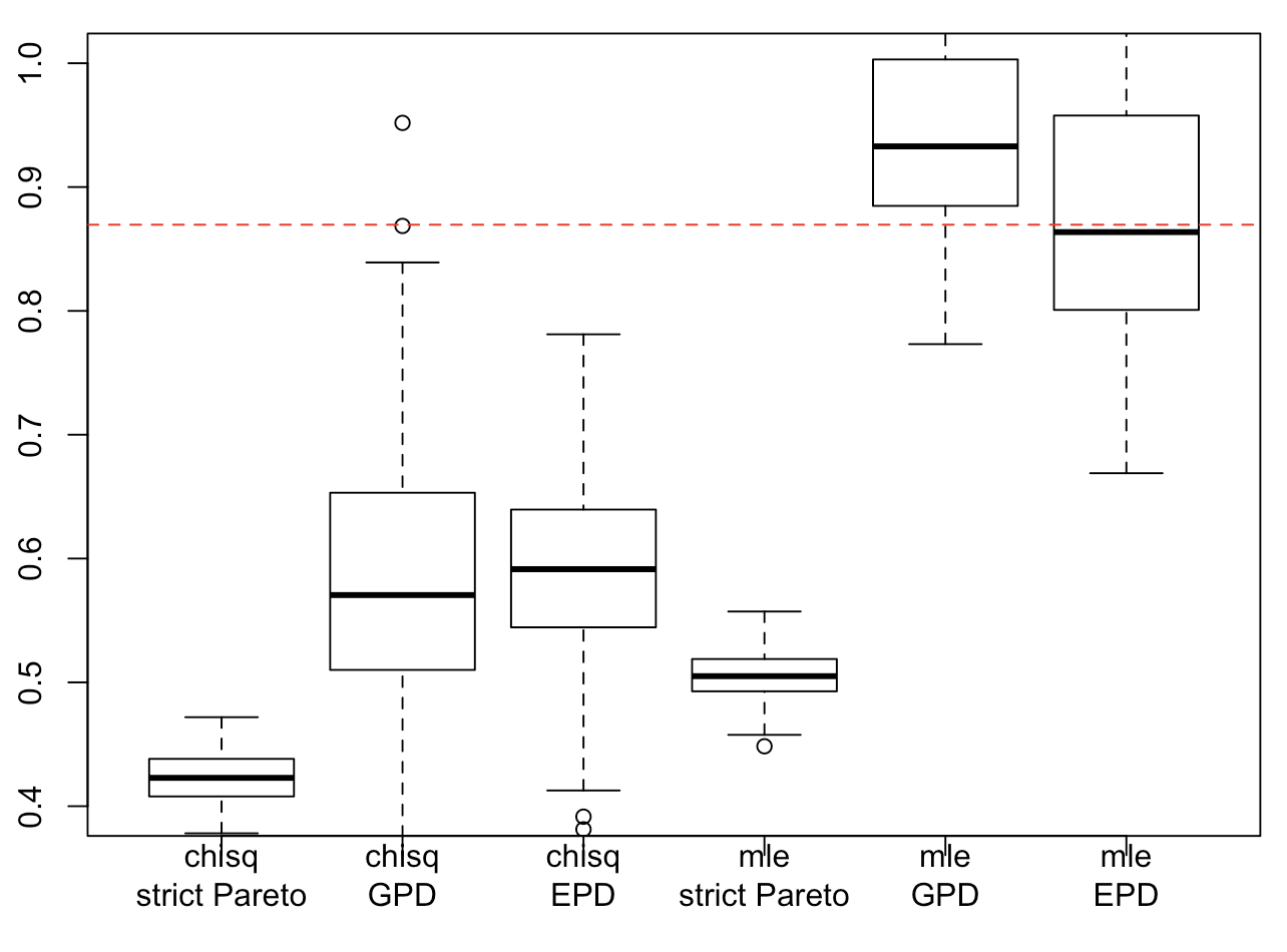
Figure 9: Simulated strict Pareto on the left ($\alpha=1.15$) and extended Pareto in the center ($\alpha=1.15$ and $\tau=-1$) and on the right ($\alpha=1.15$ and $\tau=-1.6$). Boxplot represent the distribution of $\widehat{\xi}$ over $1,000$ simulated networks (with $1,000$ nodes).

References

- Abramowitz & Stegun (1972) Abramowitz, M.; Stegun, I.A. (1972). Handbook of Mathematical Functions with Formulas, Graphs, and Mathematical Tables. New York, NBS.
- Albrecher, Beirlant & Teugels (2017) Albrecher, H., Beirlant, J. & Teugels, J.L. (2017). Reinsurance: Actuarial and Statistical Aspects. Wiley.
- Alderson et al. (2009) Alderson, D., Lun Li, W. Willinger & J.C. Doyle (2009). Understanding Internet topology: principles, models, and validation. IEEE/ACM Transactions on Networking, 13 (6), 1205–1218.
- Anderson (1980) Anderson, C.W. (1980). Local limit theorems for the maxima of discrete random variables. Mathematical Proceedings of the Cambridge Philosophical Society, 88 (1), 161–165.
- Aparicio, Villazón-Terrazas & Álvarez (2015) Aparicio, S., Villazón-Terrazas, J. & Álvarez, G. (2015). A Model for Scale-Free Networks: Application to Twitter. Entropy, 17:8, 5848–5867, doi:10.3390/e17085848
- Arnold (1983) Arnold, B.C. (1983) Pareto Distributions. International Cooperative Publishing House, Fairland, MD
- Balkema & de Haan (1974) Balkema, A. & de Haan, L. (1974). Residual life time at great age. Annals of Probability, 2, 792–804.
- Barabási & Albert (1999) Barabási, Albert-László; Albert, Réka. (1999). Emergence of scaling in random networks. Science. 286 (5439), 509–512.
- Barabási (2016) Barabási, Albert-László (2016). Network Science. Cambridge University Press. http://networksciencebook.com/
- Beirlant, Joossens & Segers (2009) Beirlant, J., Joossens, E. & Segers, J. (2009). Second-Order Refined Peaks-Over-Threshold Modelling for Heavy-Tailed Distributions. Journal of Statistical Planning and Inference, 139, 2800–2815.
- Beirlant et al. (2004) Beirlant, J., Goegebeur, Y., Teugels, J. & Segers, J. (2004). Statistics of Extremes: Theory and Applications. Wiley.
- Blitzstein & Diaconis (2010) Blitzstein, Joseph & Diaconis, Persi. A Sequential Importance Sampling Algorithm for Generating Random Graphs with Prescribed Degrees. Internet Mathematics 6 (4), 489–522.
- Broido & Clauset (2019) Broido, Anna D. & Aaron Clauset (2018). Scale-free networks are rare. Nature Communications, 10 (1017)
- Buddana & Kozubowski (2014) Buddana, A. & Kozubowski, T.J. (2014). Discrete Pareto Distributions. Economic Quality Control, 29 (2), 143–156.
- Chatterjee, Diaconis & Sly (2011) Chatterjee, Sourav; Diaconis, Persi & Sly, Allan. (2011) Random graphs with a given degree sequence. Annals of Applied Probabability, 21 (4), 1400–1435. doi:10.1214/10-AAP728
- Clauset, Cosma & Newman (2007) Clauset, Aaron, Cosma Rohilla Shalizi & M. E. J Newman (2007). Power-law distributions in empirical data. SIAM Review. 51 (4), 661–703.
- Cheng & Jiang (2001) Cheng, S. & Jiang, C. (2001) The edgeworth expansion for distributions of extreme values. Science China Mathematics 44, 427–437.
- Davison & Smith (1990) Davison, A.C.& Smith, R. L. (1990). Models for exceedances over high thresholds. Journal of the Royal Statistical Society. Series B. Methodological, 52 (3), 393–442.
- Drees (1998) Drees, H.: On smooth statistical tails functionals. Scandinavian Journal of Statistics, 25, 187–210
- Embrechts, Klüppelberg & Mikosch (1997) Embrechts, P. Klüppelberg, C. & Mikosch, C. (1997). Modelling Extremal Events. Springer Verlag.
- Gentleman et al. (2019) Gentleman, R., Whalen, E., Huber, W. & Falcon, S. (2019). graph: graph: A package to handle graph data structures. R package version 1.62.0.
- Gjoka et al. (2009) Gjoka, M., Kurant, M., Butts, C.T. & Markopoulou, A. (2009) A Walk in Facebook: Uniform Sampling of Users in Online Social Networks. arXiv:0906.0060.
- de Haan & Ferreira (2006) de Haan, L.D. & Ferreira, A. (2006). Extreme Value Theory. An Introduction. Springer.
- de Haan & Stadtmüller (1996) de Haan, L. & Stadtml̈ler, U. (1996) Generalized regular variation of second order. J. Austral. Math. Soc. A. Pure Math. 61, 381–395.
- Hall (1982) Hall, P. (1982). On some simple estimates of an exponent of regular variation. Journal of the Royal Statistical Society. Series B. Methodological, 44, 37–42.
- Hitz, Davis & Samorodnitsky (2017) Hitz, Adrien, Davis, Richard & Samorodnitsky, Gennady (2017). Discrete Extremes. arXiv:1707.05033.
- Johnson, Kotz & Balakrishnan (1994) Johnson, N.L., Kotz, S. & Balakrishnan, N. (1994) Continuous univariate distributions Vol 1. Wiley Series in Probability and Statistics.
- Krishna & Pundir (2009) Krishna, H. & Pundir, P. S. (2009). Discrete Burr and discrete Pareto distributions. Statistical Methodology, 6 (2), 177–188.
- Li et al. (2005) Li, L., Alderson, D., Doyle, J. C. & Willinger, W. (2005). Towards a theory of scale-free graphs: Definition, properties, and implications. Internet Mathematics, 2, 431–523.
- McAuley & Leskovec (2012) McAuley, J. & Leskovec, J. (2012). Learning to Discover Social Circles in Ego Networks. NIPS.
- Newman (2002) Newman, M. E. J. (2002). Random graphs as models of networks. arXiv:cond-mat/0202208.
- Pickands (1975) Pickands, J. III. (1975). Statistical inference using extreme order statistics. The Annals of Statistics, 3, 119–131.
- Shimura (2012) Shimura, T. (2012) Discretization of distributions in the maximum domain of attraction. Extremes, 15 (3), 299–317.
- Stumpf, Wiuf & May (2005) M. Stumpf, C. Wiuf, and R. May (2005). Subnets of scale-free networks are notscale-free: sampling properties of networks Proceedings of the National Academy of Sciences of the United States of America, 102: 12, 4221–4224.
- Tripathi, Venugopalan & West (2010) Tripathi, Amitabha, Venugopalan, Sushmita & West, Douglas B. (2010). A short constructive proof of the Erdös-Gallai characterization of graphic lists. Discrete Mathematics, 310 (4), 843–844, doi:10.1016/j.disc.2009.09.023.
- Voitalov et al. (2018) Voitalov, I., van der Hoorn, P., van der Hofstad, R. & Krioukov, D. (2018) Scale-free Networks Well Done. arXiv:1811.02071.
- Willinger, Alderson & Doyle (2009) Willinger, W., Alderson, D. & Doyle, J. C. (2009). Mathematics and the Internet: A source of enormous confusion and great potential. Notices of the American Mathematical Society 56, 586–599.
- Zipf (1949) Zipf, G.K. (1949) Human Behaviour and the Principle of Least Effort. Addison-Wesley, Reading,MA.