General Toeplitz matrices subject to Gaussian perturbations

Abstract.

We study the spectra of general $N\times N$ Toeplitz matrices given by symbols in the Wiener Algebra perturbed by small complex Gaussian random matrices, in the regime $N\gg 1$. We prove an asymptotic formula for the number of eigenvalues of the perturbed matrix in smooth domains. We show that these eigenvalues follow a Weyl law with probability sub-exponentially close to $1$, as $N\gg 1$, in particular that most eigenvalues of the perturbed Toeplitz matrix are close to the curve in the complex plane given by the symbol of the unperturbed Toeplitz matrix.

1. Introduction and main result

Let $a_{\nu}\in{\bf C}$, for $\nu\in{\bf Z}$ and assume that

(1.1) $$|a_{\nu}|\leq{\mathcal{O}}(1)m(\nu),$$

where $m:{\bf Z}\to]0,+\infty[$ satisfies

(1.2) $$(1+|\nu|)m(\nu)\in\ell^{1},$$

and

(1.3) $$m(-\nu)=m(\nu),\ \forall\nu\in\mathds{Z}.$$

Let

(1.4) $$p(\tau)=\sum_{-\infty}^{+\infty}a_{\nu}\tau^{\nu},$$

act on complex valued functions on ${\bf Z}$. Here $\tau$ denotes translation by 1 unit to the right: $\tau u(j)=u(j-1)$, $j\in{\bf Z}$. By (1.2) we know that $p(\tau)={\mathcal{O}}(1):\ell^{2}({\bf Z})\to\ell^{2}({\bf Z})$. Indeed, for the corresponding operator norm, we have

(1.5) $$\|p(\tau)\|\leq\sum|a_{j}|\|\tau^{j}\|=\|a\|_{\ell^{1}}\leq{\mathcal{O}}(1)\|m\|_{\ell^{1}}.$$

From the identity, $\tau(e^{ik\xi})=e^{-i\xi}e^{ik\xi}$, we define the symbol of $p(\tau)$ by

(1.6) $$p(e^{-i\xi})=\sum_{-\infty}^{\infty}a_{\nu}e^{-i\nu\xi}.$$

It is an element of the Wiener algebra [BöSi99] and by (1.2) in $C^{1}(S^{1})$.

We are interested in the Toeplitz matrix

(1.7) $$P_{N}\stackrel{{\scriptstyle\mathrm{def}}}{{=}}1_{[0,N[}p(\tau)1_{[0,N[},$$

acting on $\mathbf{C}^{N}\simeq\ell^{2}([0,N[)$, for $1\ll N<\infty$. Furthermore, we frequently identify $\ell^{2}([0,N[)$ with the space $\ell^{2}_{[0,N[}({\bf Z})$ of functions $u\in\ell^{2}({\bf Z})$ with support in $[0,N[$.

The spectra of such Toeplitz matrices have been studied thoroughly, see [BöSi99] for an overview. Let $P_{\infty}$ denote $p(\tau)$ as an operator $\ell^{2}({\bf Z})\to\ell^{2}({\bf Z})$. It is a normal operator and by Fourier series expansions, we see that the spectrum of $P_{\infty}$ is given by

(1.8) $$\sigma(P_{\infty})=p(S^{1}).$$

The restriction $P_{\mathbf{N}}=P_{\infty}|_{\ell^{2}(\mathbf{N})}$ of $P_{\infty}$ to $\ell^{2}(\mathbf{N})$, is in general no longer normal, except for specific choices of the coefficients $a_{\nu}$. The essential spectrum of the Toeplitz operator $P_{\mathbf{N}}$ is given by $p(S^{1})$ and we have pointspectrum in all loops of $p(S^{1})$ with non-zero winding number, i.e.

(1.9) $$\sigma(P_{\mathbf{N}})=p(S^{1})\cup\{z\in\mathbf{C};\mathrm{ind}_{p(S^{1})}(z)\neq 0\}.$$

By a result of Krein [BöSi99, Theorem 1.15] the winding number of $p(S^{1})$ around the point $z\not\in p(S^{1})$ is related to the Fredholm index of $P_{\mathbf{N}}-z$: $\mathrm{Ind}(P_{\mathbf{N}}-z)=-\mathrm{ind}_{p(S^{1})}(z)$.

The spectrum of the Toeplitz matrix $P_{N}$ is contained in a small neighborhood of the spectrum of $P_{\mathbf{N}}$. More precisely, for every $\epsilon>0$,

(1.10) $$\sigma(P_{N})\subset\sigma(P_{\mathbf{N}})+D(0,\epsilon)$$

for $N>0$ sufficiently large, where $D(z,r)$ denotes the open disc of radius $r$, centered at $z$. Moreover, the limit of $\sigma(P_{N})$ as $N\to\infty$ is contained in a union of analytic arcs inside $\sigma(P_{\mathbf{N}})$, see [BöSi99, Theorem 5.28].

We show in Theorem 1.1 below that after adding a small random perturbation to $P_{N}$, most of its eigenvalues will be close to the curve $p(S^{1})$ with probability very close to $1$. See Figure 1 below for a numerical illustration.

1.1. Small Gaussian perturbation

Consider the random matrix

(1.11) $$Q_{\omega}\stackrel{{\scriptstyle\mathrm{def}}}{{=}}Q_{\omega}(N)\stackrel{{\scriptstyle\mathrm{def}}}{{=}}(q_{j,k}(\omega))_{1\leq j,k\leq N}$$

with complex Gaussian law

$$(Q_{\omega})_{*}(d\mathds{P})=\pi^{-N^{2}}\mathrm{e}^{-\|Q\|_{\mathrm{HS}}^{2}}L(dQ),$$

where $L$ denotes the Lebesgue measure on $\mathbf{C}^{N\times N}$. The entries $q_{j,k}$ of $Q_{\omega}$ are independent and identically distributed complex Gaussian random variables with expectation $0$, and variance $1$.

We recall that the probability distribution of a complex Gaussian random variable $\alpha\sim\mathcal{N}_{\mathbf{C}}(0,1)$, is given by

$$\alpha_{*}(d\mathds{P})=\pi^{-1}\mathrm{e}^{-|\alpha|^{2}}L(d\alpha),$$

where $L(d\alpha)$ denotes the Lebesgue measure on $\mathbf{C}$. If $\mathds{E}$ denotes the expectation with respect to the probability measure $\mathds{P}$, then

$$\mathds{E}[\alpha]=0,\quad\mathds{E}[|\alpha|^{2}]=1.$$

We are interested in studying the spectrum of the random perturbations of the matrix $P_{N}^{0}=P_{N}$:

(1.12) $$P_{N}^{\delta}\stackrel{{\scriptstyle\mathrm{def}}}{{=}}P_{N}^{0}+\delta Q_{\omega},\quad 0\leq\delta\ll 1.$$

1.2. Eigenvalue asympotics in smooth domains

Let $\Omega\Subset\mathbf{C}$ be an open simply connected set with smooth boundary $\partial\Omega$, which is independent of $N$, satisfying

1. $\partial\Omega$ intersects $p(S^{1})$ in at most finitely many points;

2. $p(S^{1})$ does not self-intersect at these points of intersection;

3. these points of intersection are non-critical, i.e.

   $$\partial_{\zeta}p\neq 0\hbox{ on }p^{-1}(\partial\Omega\cap p(S^{1}));$$

4. $\partial\Omega$ and $p(S^{1})$ are transversal at every point of the intersection.

Theorem 1.1.

Let $p$ be as in (1.6) and let $P_{N}^{\delta}$ be as in (1.12). Let $\Omega$ be as above, satisfying conditions (1) - (4), pick a $\delta_{0}\in]0,1[$ and let $\delta_{1}>3/2$. If

(1.13) $$\mathrm{e}^{-N^{\delta_{0}}}\leq\delta\ll N^{-\delta_{1}},$$

then there exists $\varepsilon_{N}=o(1)$, as $N\to\infty$, such that

(1.14) $$\left|\#(\sigma(P^{\delta}_{N})\cap\Omega)-\frac{N}{2\pi}\int_{S^{1}\cap\,p^{-1}(\Omega)}L_{S^{1}}(d\theta)\right|\leq\varepsilon_{N}N,$$

with probability

(1.15) $$\geq 1-\mathrm{e}^{-N^{\delta_{0}}}.$$

In (1.14) we view $p$ as a map from $S^{1}$ to $\mathbf{C}$. Theorem 1.1 shows that most eigenvalues of $P_{N}^{\delta}$ can be found close to the curve $p(S^{1})$ with probability subexponentially close to $1$. This is illustrated in Figure 1 for two different symbols.

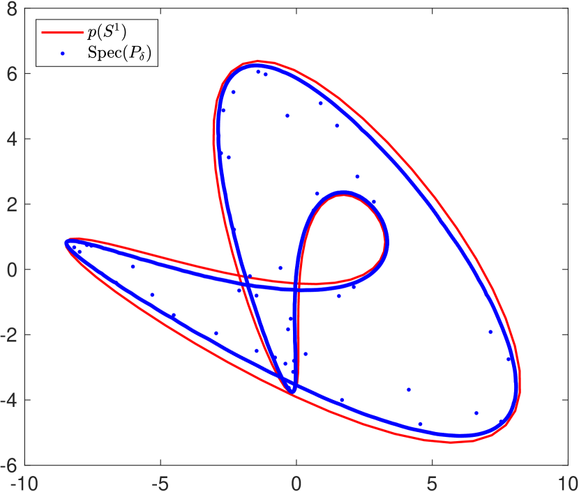
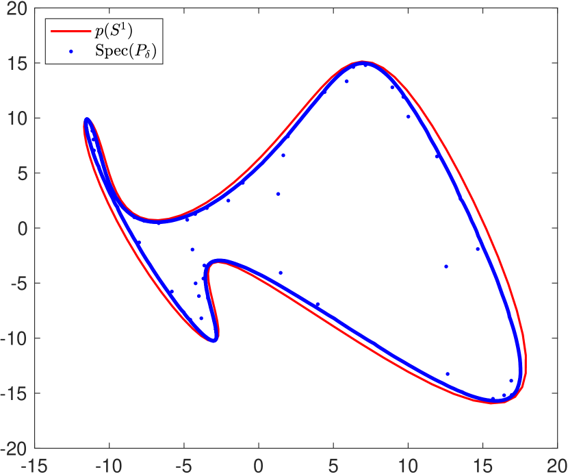
Figure 1. The left hand side shows the spectrum of the perturbed Toeplitz matrix with symbol defined in (1.16), (1.17) and the right hand side shows the spectrum of the perturbed Toeplitz matrix with symbol defined in (1.18), (1.17) The red line shows the symbol curve $p(S^{1})$.

The left hand side of Figure 1 shows the spectrum of a perturbed Toeplitz matrix with $N=2000$ and $\delta=10^{-14}$, given by the symbol $p=p_{0}+p_{1}$ where

(1.16) $$p_{0}(1/\zeta)=-\zeta^{-4}-(3+2i)\zeta^{-3}+i\zeta^{-2}+\zeta^{-1}+10\zeta+(3+i)\zeta^{2}+4\zeta^{3}+i\zeta^{4}$$

and

(1.17) $$p_{1}(1/\zeta)=\sum_{\nu\in\mathbf{Z}}a_{\nu}\zeta^{\nu},\quad a_{0}=0,~{}a_{-\nu}=0.7|\nu|^{-5}+i|\nu|^{-9},~{}a_{\nu}=-2i\nu^{-5}+0.5\nu^{-9}~{}~{}\nu\in\mathbf{N}.$$

The red line shows the curve $p(S^{1})$. The right hand side of Figure 1 similarly shows the spectrum of the perturbed Toeplitz matrix given by $p=p_{0}+p_{1}$ where $p_{1}$ is as above and

(1.18) $$p_{0}(1/\zeta)=-4\zeta^{1}-2i\zeta^{2}+2i\zeta^{-1}-\zeta^{-2}+2\zeta^{-3}.$$

In our previous work [SjVo19], we studied Toeplitz matrices with a finite number of bands, given by symbols of the form

(1.19) $$p(\tau)=\sum_{j=-N_{-}}^{N_{+}}a_{j}\tau^{j},\quad a_{-N_{-}},a_{-N_{-}+1},\dots,a_{N_{+}}\in\mathbf{C},\ a_{\pm N_{\pm}}\neq 0.$$

In this case the symbols are analytic functions on $S^{1}$ and we are able to provide in [SjVo19, Theorem 2.1] a version of Theorem 1.1 with a much sharper remainder estimate. See also [Sj19, SjVo16], concerning the special cases of large Jordan block matrices $p(\tau)=\tau^{-1}$ and large bi-diagonal matrices $p(\tau)=a\tau+b\tau^{-1}$, $a,b\in\mathbf{C}$. However, Figure 1 suggests that one could hope for a better remainder estimate in Theorem 1.1 as well.

1.3. Convergence of the empirical measure and related results

An alternative way to study the limiting distribution of the eigenvalues of $P_{N}^{\delta}$, up to errors of $o(N)$, is to study the empirical measure of eigenvalues, defined by

(1.20) $$\xi_{N}\stackrel{{\scriptstyle\mathrm{def}}}{{=}}\frac{1}{N}\sum_{\lambda\in\mathrm{Spec}(P_{N}^{\delta})}\delta_{\lambda}$$

where the eigenvalues are counted including multiplicity and $\delta_{\lambda}$ denotes the Dirac measure at $\lambda\in\mathbf{C}$. For any positive monotonically increasing function $\phi$ on the positive reals and random variable $X$, Markov’s inequality states that $\mathds{P}[|X|\geq\varepsilon]\leq\phi(\varepsilon)^{-1}\mathds{E}[\phi(|X|)]$, assuming that the last quantity is finite. This yields that for $C_{1}>0$ large enough

(1.21) $$\mathds{P}[\|Q_{\omega}\|_{\mathrm{HS}}\leq\sqrt{C_{1}N}]\geq 1-\mathrm{e}^{-N}.$$

If $\delta\leq N^{-1}$, then (1.5) and the the Borel-Cantelli Theorem shows that, almost surely, $\xi_{N}$ has compact support for $N>0$ sufficiently large.

We will show that, almost surely, $\xi_{N}$ converges weakly to the push-forward of the uniform measure on $S^{1}$ by the symbol $p$.

Theorem 1.2.

Let $\delta_{0}\in]0,1[$, let $\delta_{1}>3/2$ and let $p$ be as in (1.4). If (1.13) holds, i.e.

$$\mathrm{e}^{-N^{\delta_{0}}}\leq\delta\ll N^{-\delta_{1}}$$

then, almost surely,

(1.22) $$\xi_{N}\rightharpoonup p_{*}\left(\frac{1}{2\pi}L_{S^{1}}\right),\quad N\to\infty,$$

weakly, where $L_{S^{1}}$ denotes the Lebesgue measure on $S^{1}$.

This result generalizes [SjVo19, Corollary 2.2] from the case of Toeplitz matrices with a finite number of bands to the general case (1.4).

Similar results to Theorem 1.2 have been proven in various settings. In [BaPaZe18a, BaPaZe18b], the authors consider the special case of band Toeplitz matrices, i.e. $P_{N}$ with $p$ as in (1.19). In this case they show that the convergence (1.22) holds weakly in probability for a coupling constant $\delta=N^{-\gamma}$, with $\gamma>1/2$. Furthermore, they prove a version of this theorem for Toeplitz matrices with non-constant coefficients in the bands, see [BaPaZe18a, Theorem 1.3, Theorem 4.1]. They follow a different approach than we do: They compute directly the $\log|\det\mathcal{M}_{N}-z|$ by relating it to $\log|\det M_{N}(z)|$, where $M_{N}(z)$ is a truncation of $M_{N}-z$, where the smallest singular values of $M_{N}-z$ have been excluded. The level of truncation however depends on the strength of the coupling constant and it necessitates a very detailed analysis of the small singular values of $M_{N}-z$.

In the earlier work [GuWoZe14], the authors prove that the convergence (1.22) holds weakly in probability for the Jordan bloc matrix $P_{N}$ with $p(\tau)=\tau^{-1}$ (1.4) and a perturbation given by a complex Gaussian random matrix whose entries are independent complex Gaussian random variables whose variances vanishes (not necessarily at the same speed) polynomially fast, with minimal decay of order $N^{-1/2+}$. See also [DaHa09] for a related result.

In [Wo16], using a replacement principle developed in [TaVuKr10], it was shown that the result of [GuWoZe14] holds for perturbations given by complex random matrices whose entries are independent and identically distributed random complex random variables with expectation $0$ and variance $1$ and a coupling constant $\delta=N^{-\gamma}$, with $\gamma>2$.

Acknowledgments

The first author acknowledges support from the 2018 S. Bergman award. The second author was supported by a CNRS Momentum fellowship. We are grateful to Ofer Zeitouni for his interest and a remark which lead to a better presentation of this paper.

2. The unperturbed operator

We are interested in the Toeplitz matrix

(2.1) $$P_{N}=1_{[0,N[}p(\tau)1_{[0,N[}:\ell^{2}([0,N[)\to\ell^{2}([0,N[)$$

for $1\ll N<\infty$, see also (1.7). Here we identify $\ell^{2}([0,N[)$ with the space $\ell^{2}_{[0,N[}({\bf Z})$ of functions $u\in\ell^{2}({\bf Z})$ with support in $[0,N[$. Sometimes we write $P_{N}=P_{[0,N[}$ and identify $P_{N}$ with $P_{I}=1_{I}p(\tau)1_{I}$ where $I=I_{N}$ is any interval in ${\bf Z}$ of “length” $|I|=\#I=N$.

Let $P_{\bf N}=P_{[0,+\infty[}$ and let $P_{{\bf Z}/\widetilde{N}{\bf Z}}$ denote $P=p(\tau)$, acting on $\ell^{2}({\bf Z}/\widetilde{N}{\bf Z})$ which we identify with the space of $\widetilde{N}$-periodic functions on ${\bf Z}$. Here $\widetilde{N}\geq 1$. Using the the discrete Fourier transform, we see that

(2.2) $$\sigma(P_{{\bf Z}/\widetilde{N}{\bf Z}})=p(S_{\widetilde{N}}),$$

where $S_{\widetilde{N}}$ is the dual of ${\bf Z}/\widetilde{N}\mathbf{Z}$ and given by

$$S_{\widetilde{N}}=\{e^{ik2\pi/\widetilde{N}};\,0\leq k<\widetilde{N}\}.$$

Let

(2.3) $$p_{N}(\tau)=\sum_{|\nu|\leq N}a_{\nu}\tau^{\nu}=\sum_{\nu\in{\bf Z}}a_{\nu}^{N}\tau^{\nu},\ \ a_{\nu}^{N}=1_{[-N,N]}(\nu)a_{\nu}.$$

and notice that

(2.4) $$P_{N}=1_{[0,N[}\,p_{N}(\tau)1_{[0,N[}.$$

We now consider $[0,N[$ as an interval $I_{N}$ in ${\bf Z}/\widetilde{N}{\bf Z}$, $\widetilde{N}=N+M$, where $M\in\{1,2,..\}$ will be fixed and independent of $N$. The matrix of $P_{N}$, indexed over $I_{N}\times I_{N}$ is then given by

(2.5) $$P_{N}(j,k)=a^{N}_{\widetilde{j}-\widetilde{k}},\ j,k\in I_{N}\subset{\bf Z}/\widetilde{N}Z,$$

where $\widetilde{j},\widetilde{k}\in{\bf Z}$ are the preimages of $j,k$ under the projection ${\bf Z}\to{\bf Z}/\widetilde{N}{\bf Z}$, that belong to the interval $[0,N[\subset{\bf Z}$.

Let $\widetilde{P}_{N}$ be given by the formula (2.4), with the difference that we now view $\tau$ as a translation on $\ell^{2}({\bf Z}/\widetilde{N}{\bf Z})$:

(2.6) $$\widetilde{P}_{N}=1_{I_{N}}p_{N}(\tau)1_{I_{N}}.$$

The matrix of $\widetilde{P}_{N}$ is given by

(2.7) $$\widetilde{P}_{N}(j,k)=\sum_{\nu\in{\bf Z},\atop\nu\equiv j-k\,\mathrm{mod\,}\widetilde{N}{\bf Z}}a_{\nu}^{N},\quad j,k\in I_{N}.$$

Alternatively, if we let $\widetilde{j},\widetilde{k}$ be the preimages in $[0,N[$ of $j,k\in I_{N}$, then

(2.8) $$\widetilde{P}_{N}(j,k)=\sum_{\widehat{j}\in{\bf Z};\ \widehat{j}\equiv\widetilde{j}\,\mathrm{mod\,}\widetilde{N}{\bf Z}}a^{N}_{\widehat{j}-\widetilde{k}}.$$

Recall that the terms in (2.7), (2.8) with $|\nu|>N$ or $|\widehat{j}-\widetilde{k}|>N$ do vanish. This implies that with $\widetilde{j}$, $\widetilde{k}$ as in (2.8),

(2.9) $$\widetilde{P}_{N}(j,k)-P_{N}(j,k)=a^{N}_{\widetilde{j}-\widetilde{N}-\widetilde{k}}+a^{N}_{\widetilde{j}+\widetilde{N}-\widetilde{k}}.$$

Here

$$\begin{split}&\widetilde{j}-\widetilde{N}\in[0,N[-\widetilde{N}=[-\widetilde{N},N-\widetilde{N}[=[-N-M,-M[,\\ &\widetilde{j}+\widetilde{N}\in[0,N[+\widetilde{N}=[\widetilde{N},N+\widetilde{N}[=[N+M,2N+M[.\end{split}$$

Since $\widetilde{k}\in[0,N[$ we have for the first term in (2.9) that $|\widetilde{j}-\widetilde{N}-\widetilde{k}|=\widetilde{k}+M+(N-\widetilde{j})$ with nonnegative terms in the last sum. Similarly for the second term in (2.9), we have $|\widetilde{j}+\widetilde{N}-\widetilde{k}|=\widetilde{j}+M+(N-\widetilde{k})$ where the terms in the last sum are all $\geq 0$.

It follows that the trace class norm of $P_{N}-\widetilde{P}_{N}$ is bounded from above by

$$\begin{split}\sum_{j<-M,\ k\geq 0}|a_{j-k}|&+\sum_{j\geq N+M,\ k<N}|a_{j-k}|=\sum_{k\geq 0,\ j\leq-M}|a_{j-k}|+\sum_{k\leq 0,\ j\geq M}|a_{j-k}|\\ &\leq 2C\sum_{k=0}^{\infty}\sum_{j=0}^{\infty}m(M+k+j)=2C\sum_{k=0}^{\infty}(k+1)m(M+k)\\ &=2C\sum_{k=M}^{\infty}(k+1-M)m(k).\end{split}$$

By (1.2), it follows that

(2.10) $$\|P_{N}-\widetilde{P}_{N}\|_{\mathrm{tr}}\leq 2C\sum_{k=M}^{+\infty}(k+1-M)m(k)\to 0,\ M\to\infty,$$

uniformly with respect to $N$.

3. A Grushin problem for $P_{N}-z$

Let $K\Subset\mathbf{C}$ be an open relatively compact set and let $z\in K$. Consider

(3.1) $$J=[-M,0[,\ I_{N}=[0,N[$$

as subsets of ${\bf Z}/(N+M){\bf Z}$ so that

$$J\cup I_{N}={\bf Z}/(N+M){\bf Z}=:{\bf Z}_{N+M}$$

is a partition. Recall (2.3), (2.6) and consider

$$p_{N}(\tau)-z:\ell^{2}({\bf Z}_{N+M})\to\ell^{2}({\bf Z}_{N+M})$$

and write this operator as a $2\times 2$ matrix

(3.2) $$p_{N}-z=\begin{pmatrix}\widetilde{P}_{N}-z&R_{-}\\ R_{+}&R_{+-}(z)\end{pmatrix},$$

induced by the orthogonal decomposition

(3.3) $$\ell^{2}({\bf Z}_{N+M})=\ell^{2}(I_{N})\oplus\ell^{2}(J).$$

The operator $p_{N}(\tau)$ is normal and we know by (2.2) that its spectrum is

(3.4) $$\sigma(p_{N}(\tau))=p_{N}(S_{N+M}).$$

Replacing $\widetilde{P}_{N}$ in (3.2) by $P_{N}$ (2.4), we put

(3.5) $${\mathcal{P}}_{N}(z)=\begin{pmatrix}P_{N}-z&R_{-}\\ R_{+}&R_{+-}(z)\end{pmatrix}.$$

Then, by (2.10),

(3.6) $$\|{\mathcal{P}}_{N}(z)-(p_{N}-z)\|_{\mathrm{tr}}\leq 2C\sum_{k=M}^{+\infty}(k+1-M)m(k)=:\epsilon(M).$$

If $\epsilon(M)<\mathrm{dist\,}(z,p_{N}(S_{N+M}))=:d_{N}(z)$, then ${\mathcal{P}}(z)$ is bijective and

(3.7) $$\|{\mathcal{P}}_{N}(z)^{-1}\|\leq\frac{1}{d_{N}(z)-\epsilon(M)}.$$

Write,

$$\begin{split}{\mathcal{P}}_{N}(z)&=p_{N}(\tau)-z+{\mathcal{P}}_{N}(z)-(p_{N}(\tau)-z)\\ &=(p_{N}(\tau)-z)\left(1+(p_{N}(\tau)-z)^{-1}({\mathcal{P}}_{N}(z)-(p_{N}(\tau)-z))\right).\end{split}$$

Here,

$$\begin{split}\big{|}\det\big{(}1+(p_{N}(\tau)-z)^{-1}&({\mathcal{P}}_{N}(z)-(p_{N}(\tau)-z))\big{)}\big{|}\\ &\leq\exp\|(p_{N}(\tau)-z)^{-1}({\mathcal{P}}_{N}(z)-(p_{N}(\tau)-z))\|_{\mathrm{tr}}\\ &\leq\exp(\epsilon(M)/d_{N}(z)),\end{split}$$

so

(3.8) $$|\det{\mathcal{P}}_{N}(z)|\leq|\det(p_{N}(\tau)-z)|\,e^{\epsilon(M)/d_{N}(z)}.$$

Similarly from

$$\begin{split}p_{N}(\tau)-z&={\mathcal{P}}_{N}(z)+p_{N}(\tau)-z-{\mathcal{P}}_{N}(z)\\ &={\mathcal{P}}_{N}(z)\left(1+{\mathcal{P}}_{N}(z)^{-1}(p_{N}(\tau)-z-{\mathcal{P}}_{N}(z)\right),\end{split}$$

we get

(3.9) $$|\det(p_{N}(\tau)-z)|\leq|\det{\mathcal{P}}_{N}(z)|e^{\frac{\epsilon(M)}{d_{N}(z)-\epsilon(M)}}.$$

In analogy with (3.5), we write

(3.10) $${\mathcal{P}}_{N}(z)^{-1}={\mathcal{E}}_{N}(z)=\begin{pmatrix}E^{N}&E_{+}^{N}\\ E_{-}^{N}&E_{-+}^{N}\end{pmatrix}:\ \ell^{2}(I_{N})\oplus\ell^{2}(J)\to\ell^{2}(I_{N})\oplus\ell^{2}(J),$$

where $J$, $I_{N}$ were defined in (3.1), still viewed as intervals in ${\bf Z}_{N+M}$. From (3.7) we get for the respective operator norms:

(3.11) $$\|E^{N}\|,\|E^{N}_{+}\|,\|E^{N}_{-}\|,\|E^{N}_{-+}\|\leq(d_{N}(z)-\epsilon(M))^{-1}.$$

4. Second Grushin problem

We begin with a result, which is a generalization of [SjZw07, Proposition 3.4] to the case where $R_{+-}\neq 0$.

Proposition 4.1.

Let ${\mathcal{H}}_{1},{\mathcal{H}}_{2},{\mathcal{H}}_{\pm},{\mathcal{S}}_{\pm}$ be Banach spaces. If

(4.1) $${\mathcal{P}}=\begin{pmatrix}P&R_{-}\\ R_{+}&R_{+-}\end{pmatrix}:{\mathcal{H}}_{1}\times{\mathcal{H}}_{-}\to{\mathcal{H}}_{2}\times{\mathcal{H}}_{+}$$

is bijective with bounded inverse,

$${\mathcal{E}}=\begin{pmatrix}E&E_{+}\\ E_{-}&E_{-+}\end{pmatrix}:{\mathcal{H}}_{2}\times{\mathcal{H}}_{+}\to{\mathcal{H}}_{1}\times{\mathcal{H}}_{-},$$

and if

(4.2) $${\mathcal{S}}=\begin{pmatrix}E_{-+}&S_{-}\\ S_{+}&0\end{pmatrix}:{\mathcal{H}}_{+}\times{\mathcal{S}}_{-}\to{\mathcal{H}}_{-}\times{\mathcal{S}}_{+}$$

is bijective with bounded inverse

$${\mathcal{F}}=\begin{pmatrix}F&F_{+}\\ F_{-}&F_{-+}\end{pmatrix}:{\mathcal{H}}_{-}\times{\mathcal{S}}_{+}\to{\mathcal{H}}_{+}\times{\mathcal{S}}_{-},$$

then

(4.3) $${\mathcal{T}}=\begin{pmatrix}P&R_{-}S_{-}\\ S_{+}R_{+}&S_{+}R_{+-}S_{-}\end{pmatrix}=:\begin{pmatrix}T&T_{-}\\ T_{+}&T_{+-}\end{pmatrix}:{\mathcal{H}}_{1}\times{\mathcal{S}}_{-}\to{\mathcal{H}}_{2}\times{\mathcal{S}}_{+}$$

is bijective with the bounded inverse

(4.4) $${\mathcal{G}}=\begin{pmatrix}G&G_{+}\\ G_{-}&G_{-+}\end{pmatrix}=\begin{pmatrix}E-E_{+}FE_{-}&E_{+}F_{+}\\ F_{-}E_{-}&-F_{-+}\end{pmatrix}:{\mathcal{H}}_{2}\times{\mathcal{S}}_{+}\to{\mathcal{H}}_{1}\times{\mathcal{S}}_{-}$$

Proof.

We can essentially follow the proof of [SjZw07, Proposition 3.4]. We need to solve

(4.5) $$\begin{cases}Pu+R_{-}S_{-}u_{-}=v\\ S_{+}R_{+}u+S_{+}R_{+-}S_{-}u_{-}=v_{+}.\end{cases}$$

Putting $\widetilde{v}_{+}=R_{+}u+R_{+-}S_{-}u_{-}$, the first equation is equivalent to

$$\begin{cases}Pu+R_{-}S_{-}u_{-}=v\\ R_{+}u+R_{+-}S_{-}u_{-}=\widetilde{v}_{+},\end{cases}\quad\text{i.e.}\quad\mathcal{P}\begin{pmatrix}u\\ S_{-}u_{-}\\ \end{pmatrix}=\begin{pmatrix}v\\ \widetilde{v}_{+}\\ \end{pmatrix},$$

and hence to

(4.6) $$\begin{cases}u=Ev+E_{+}\widetilde{v}_{+}\\ S_{-}u_{-}=E_{-}v+E_{-+}\widetilde{v}_{+}.\end{cases}$$

Therefore, we can replace $u$ by $\widetilde{v}_{+}$ and (4.5) is equivalent to

(4.7) $$\begin{pmatrix}E_{-+}&S_{-}\\ S_{+}&0\\ \end{pmatrix}\begin{pmatrix}\widetilde{v}_{+}\\ -u_{-}\\ \end{pmatrix}=\begin{pmatrix}-E_{-}v\\ v_{+}\\ \end{pmatrix}$$

which can be solved by $\mathcal{F}$. Hence, (4.7) is equivalent to

$$\begin{cases}\widetilde{v}_{+}=-FE_{-}v+F_{+}v_{+}\\ -u_{-}=-F_{-}E_{-}v+F_{-+}v_{+},\end{cases}$$

and (4.6) gives the unique solution of (4.5)

$$\begin{cases}u=(E-E_{+}FE_{-})v+E_{+}F_{+}v_{+}\\ u_{-}=F_{-}E_{-}v-F_{-+}v_{+}.\end{cases}\qed$$

4.1. Grushin problem for $E_{-+}(z)$

We want to apply Proposition 4.1 to ${\mathcal{P}}={\mathcal{P}}(z)={\mathcal{P}}_{N}(z)$ in (3.5) with the inverse ${\mathcal{E}}={\mathcal{E}}_{N}(z)$ in (3.10), where we sometimes drop the index $N$. We begin by constructing an invertible Grushin problem for $E_{-+}$:

Let $0\leq t_{1}\leq\dots\leq t_{M}$ denote the singular values of $E_{-+}(z)$. Let $e_{1},\dots,e_{M}$ denote an orthonormal basis of eigenvectors of $E_{-+}^{*}E_{-+}$ associated to the eigenvalues $t_{1}^{2}\leq\dots\leq t_{M}^{2}$. Since $E_{-+}$ is Fredholm of index $0$, we have that $\dim\mathcal{N}(E_{-+}(z))=\dim\mathcal{N}(E_{-+}^{*}(z))$. Using the spectral decomposition $\ell^{2}(J)=\mathcal{N}(E_{-+}^{*}E_{-+})\oplus_{\perp}\mathcal{R}(E_{-+}^{*}E_{-+})$ together with the fact that $\mathcal{N}(E_{-+}^{*}E_{-+})=\mathcal{N}(E_{-+})$ and $\mathcal{R}(E_{-+}^{*})=\mathcal{N}(E_{-+})^{\perp}$, it follows that $\mathcal{R}(E_{-+}^{*})=\mathcal{R}(E_{-+}^{*}E_{-+})$. Similarly, we get that $\mathcal{R}(E_{-+})=\mathcal{R}(E_{-+}E_{-+})^{*}$. One then easily checks that $E_{-+}:\mathcal{R}(E_{-+}^{*}E_{-+})\to\mathcal{R}(E_{-+}E_{-+}^{*})$ is a bijection. Similarly, we get that $E_{-+}^{*}:\mathcal{R}(E_{-+}E_{-+}^{*})\to\mathcal{R}(E_{-+}^{*}E_{-+})$ is a bijection. Let $f_{1},\dots,f_{M_{0}}$ denote an orthonormal basis of $\mathcal{N}(E_{-+}^{*}(z))$ and set

$$f_{j}=t_{j}^{-1}E_{-+}e_{j},\quad j=M_{0}+1,\dots,M.$$

Then, $f_{1},\dots,f_{M}$ is an orthonormal basis of $\ell^{2}(J)$ comprised of eigenfunctions of $E_{-+}E_{-+}^{*}$ associated with the eigenvalues $t_{1}^{2}\leq\dots\leq t_{M}^{2}$. In particular, $\sigma(E_{-+}E_{-+}^{*})=\sigma(E_{-+}^{*}E_{-+})$ and

(4.8) $$E_{-+}e_{j}=t_{j}f_{j},\quad E_{-+}^{*}f_{j}=t_{j}e_{j},\quad j=1,\dots,M.$$

Let $0\leq t_{1}\leq...\leq t_{k}$ be the singular values of $E_{-+}(z)$ in the interval $[0,\tau]$ for $\tau>0$ small. Let ${\mathcal{S}}_{+},\,{\mathcal{S}}_{-}\subset\ell^{2}(J)$ be the corresponding (sums of) spectral subspaces for $E_{-+}^{*}E_{-+}$ and $E_{-+}E_{-+}^{*}$ respectively, corresponding to the eigenvalues $t_{1}^{2}\leq t_{2}^{2}\leq...\leq t_{k}^{2}$ in $[0,\tau^{2}]$. Using (4.8), we see that the restrictions (denoted by the same symbols)

$$E_{-+}:{\mathcal{S}}_{+}\to{\mathcal{S}}_{-},\ E_{-+}^{*}:{\mathcal{S}}_{-}\to{\mathcal{S}}_{+},$$

have norms $\leq\tau$. Also,

(4.9) $$E_{-+}:{\mathcal{S}}_{+}^{\perp}\to{\mathcal{S}}_{-}^{\perp},\ E_{-+}^{*}:{\mathcal{S}}_{-}^{\perp}\to{\mathcal{S}}_{+}^{\perp}$$

are bijective with inverses of norm $\leq 1/\tau$.

Let $S_{+}$ be the orthogonal projection onto ${\mathcal{S}}_{+}$, viewed as an operator $\ell^{2}(J)\to{\mathcal{S}}_{+}$, whose adjoint is the inclusion map ${\mathcal{S}}_{+}\to\ell^{2}(J)$. Let $S_{-}:{\mathcal{S}}_{-}\to\ell^{2}(J)$ be the inclusion map. Let ${\mathcal{S}}$ be the operator in (4.2) with ${\mathcal{H}}_{\pm}=\ell^{2}(J)$, corresponding to the problem

(4.10) $$\begin{cases}E_{-+}g+S_{-}g_{-}=h\in\ell^{2}(J),\\ S_{+}g=h_{+}\in{\mathcal{S}}_{+},\end{cases}$$

for the unknowns $g\in\ell^{2}(J)$, $g_{-}\in{\mathcal{S}}_{-}$. Using the orthogonal decompositions,

$$\ell^{2}(J)={\mathcal{S}}_{+}^{\perp}\oplus{\mathcal{S}}_{+},\ \ell^{2}(J)={\mathcal{S}}_{-}^{\perp}\oplus{\mathcal{S}}_{-},$$

we write $g=\sum_{1}^{k}g_{j}e_{j}+g^{\perp}$ and $h=\sum_{1}^{k}h_{j}f_{j}+h^{\perp}$. Then, (4.10) is equivalent to

$$\begin{cases}g^{\perp}=(E_{-+})^{-1}h^{\perp}\\ \begin{pmatrix}g_{j}\\ g_{-}^{j}\end{pmatrix}=\begin{pmatrix}0&1\\ 1&-t_{j}\end{pmatrix}\begin{pmatrix}h_{j}\\ h_{+}^{j}\end{pmatrix},~{}~{}j=1,\dots,M,\end{cases}$$

where we also used that $g_{-}=\sum_{1}^{k}g_{-}^{j}f_{j}$ and $h_{+}=\sum_{1}^{k}h_{+}^{j}e_{j}$. It follows that

(4.11) $$\begin{cases}g=(E_{-+})^{-1}h^{\perp}+\sum_{1}^{k}h_{+}^{j}e_{j}\\ g_{-}=\sum_{1}^{k}h^{j}f_{j}-\sum_{1}^{k}t_{j}h_{+}^{j}f_{j}.\end{cases}$$

Hence, the unique solution to (4.10) is given by

(4.12) $$\begin{pmatrix}g\\ g_{-}\end{pmatrix}={\mathcal{F}}\begin{pmatrix}h\\ h_{+}\end{pmatrix}=\begin{pmatrix}F&F_{+}\\ F_{-}&F_{-+}\end{pmatrix}\begin{pmatrix}h\\ h_{+}\end{pmatrix},$$

where

(4.13) $$\begin{split}&F=E_{-+}^{-1}\Pi_{{\mathcal{S}}_{-}^{\perp}},\ \ F_{+}=S_{+}^{*},\\ &F_{-}=S_{-}^{*},\ \ F_{-+}=-{{E_{-+}}_{|}}_{{\mathcal{S}}_{+}}:\,{\mathcal{S}}_{+}\to{\mathcal{S}}_{-}.\end{split}$$

Here $\Pi_{B}$ denotes the orthogonal projection onto the subspace $B$ of $A$, viewed as a self-adjoint operator $A\to A$. Notice that $F=\Pi_{\mathcal{S}_{+}^{\perp}}F$ and that

(4.14) $$F_{-+}=-\sum_{1}^{k}t_{j}f_{j}\circ e_{j}^{*}.$$

Using as well (4.9), we have

(4.15) $$\|F\|\leq 1/\tau,\ \|F_{+}\|,\|F_{-}\|\leq 1,\|F_{-+}\|\leq\tau.$$

4.2. Composing the Grushin problems

From now on we assume that

(4.16) $$0<\alpha\ll 1,\ \ \epsilon(M)\leq\alpha/2,$$

and the estimates below will be uniformly valid for $z\in K\setminus\gamma_{\alpha}$, $N\gg 1$, where $K$ is some fixed relatively compact open set in ${\bf C}$ and

(4.17) $$\gamma_{\alpha}=\{z\in{\bf C};\,\mathrm{dist\,}(z,\gamma)\leq\alpha\},\ \ \gamma=p(S^{1}).$$

We apply Proposition 4.1 to ${\mathcal{P}_{N}}$ in (3.5) with the inverse $\mathcal{E}_{N}$ in (3.10), and to $\mathcal{S}$ defined in (4.10) with inverse in $\mathcal{F}$ in (4.12). Let $z\in K\backslash\gamma_{\alpha}$, then

(4.18) $${\mathcal{T}_{N}}=\begin{pmatrix}P_{N}-z&R_{-}S_{-}\\ S_{+}R_{+}&S_{+}R_{+-}S_{-}\end{pmatrix}=\begin{pmatrix}T&T_{-}\\ T_{+}&T_{+-}\end{pmatrix}:L^{2}(I_{N})\times{\mathcal{S}}_{-}\to L^{2}(I_{N})\times{\mathcal{S}}_{+},$$

defined as in (4.3), is bijective with the bounded inverse

(4.19) $${\mathcal{G}_{N}}=\begin{pmatrix}G^{N}&G_{+}^{N}\\ G_{-}^{N}&G_{-+}^{N}\end{pmatrix}=\begin{pmatrix}E^{N}-E_{+}^{N}FE_{-}^{N}&E_{+}^{N}F_{+}\\ F_{-}E_{-}^{N}&-F_{-+}\end{pmatrix}.$$

Since $S_{\pm}$ have norms $\leq 1$, we get

(4.20) $$\|T_{\pm}\|\leq\|R_{\pm}\|=\mathcal{O}(1),$$

uniformly in $N$, $\alpha$ and $z\in K$. Also, since the norms of $E^{N},E_{+}^{N},E_{-}^{N}$ are $\leq 2/\alpha$ (uniformly as $N\to\infty$) by (3.11), we get from (4.4), (4.15), that

(4.21) $$\|G^{N}\|\leq\frac{2}{\alpha}+\frac{4}{\tau\alpha^{2}},\ \|G^{N}_{-+}\|\leq\tau,\ \|G^{N}_{\pm}\|\leq\frac{2}{\alpha}.$$

Proposition 4.2.

Let $K\Subset\mathbf{C}$ be an open relatively compact set, let $z\in K\backslash\gamma_{\alpha}$, and let $\tau>0$ be as in the definition of the Grushin problem (4.10). Then, for $\tau>0$ small enough, depending only on $K$, we have that $G_{+}$ is injective and $G_{-}$ is surjective. Moreover, there exists a constant $C>0$, depending only on $K$, such that for all $z\in K\backslash\gamma_{\alpha}$ the singular values $s_{j}^{+}$ of $G_{+}$, and $s_{j}^{-}$ of $G_{-}^{*}$ satisfy

(4.22) $$\frac{1}{C}\leq s_{j}^{\pm}\leq\frac{2}{\alpha},\quad 1\leq j\leq k(z)=\mathrm{rank}(G_{\pm}).$$

Proof.

We begin with the injectivity of $G_{+}$. From

(4.23) $$\begin{pmatrix}P&T_{-}\\ T_{+}&T_{+-}\end{pmatrix}\begin{pmatrix}G&G_{+}\\ G_{-}&G_{-+}\end{pmatrix}=1,$$

we have $T_{+}G_{+}+T_{+-}G_{-+}=1$ which we write $T_{+}G_{+}=1-T_{+-}G_{-+}$. Here

$$\|T_{+-}G_{-+}\|\leq\|R_{+-}\|\tau={\mathcal{O}}(\tau),$$

where we used that $\|R_{-+}\|\leq\|p(\tau)-z\|=\mathcal{O}(1)\|m\|_{\ell^{1}}$, thus the error term above only depends on $K$. Choosing $\tau>0$ small enough, depending on $K$ but not on $N$, we get that $\|T_{+-}G_{+-}\|\leq 1/2$. Then $1-T_{+-}G_{-+}$ is bijective with $\|(1-T_{+-}G_{-+})^{-1}\|\leq 2$ and $G_{+}$ has the left inverse

(4.24) $$(1-T_{+-}G_{-+})^{-1}T_{+}$$

of norm $\leq 2\|R_{+}\|={\mathcal{O}}(1)$, depending only on $K$.

Now we turn to the surjectivity of $G_{-}$. From

$$\begin{pmatrix}G&G_{+}\\ G_{-}&G_{-+}\end{pmatrix}\begin{pmatrix}P-z&T_{-}\\ T_{+}&T_{+-}\end{pmatrix}=1,$$

we get

$$\begin{pmatrix}(P-z)^{*}&T_{+}^{*}\\ T_{-}^{*}&T_{+-}^{*}\end{pmatrix}\begin{pmatrix}G^{*}&G_{-}^{*}\\ G_{+}^{*}&G_{-+}^{*}\end{pmatrix}=1,$$

and as above we then see that $G_{-}^{*}$ has the left inverse $(1-T_{+-}^{*}G_{-+}^{*})^{-1}T_{-}^{*}$. Hence $G_{-}$ has the right inverse

(4.25) $$T_{-}(1-G_{-+}T_{+-})^{-1},$$

of norm $\leq 2\|R_{-}\|=\mathcal{O}(1)$, depending only on $K$.

The lower bound on the singular values follows from the estimates on the left inverses of $G_{+}$ and $G_{-}^{*}$, and the upper bound follows from (4.21). ∎

5. Determinants

We continue working under the assumptions (4.16), (4.17). Additionally, we fix $\tau>0$ sufficiently small (depending only on the fixed relatively compact set $K\Subset\mathbf{C}$) so that $\|T_{+-}G_{-+}\|$, $\|G_{-+}T_{+-}\|$ (both $={\mathcal{O}}(\tau)$) are $\leq 1/2$, which implies that $G_{+}$ is injective and $G_{+}$ is surjective, see Proposition 4.2.

From now on we will work with $z\in K\backslash\gamma_{\alpha}$. The constructions and estimates in Section 3 are then uniform in $z$ for $N\gg 1$ and the same holds for those in Section 4.

Remark 5.1.

To get the $o(N)$ error term in Theorem 1.1, we will take $\alpha>0$ arbitrarily small, and $M>1$ large enough (but fixed) so that $\varepsilon(M)\leq\alpha/2$, see (2.10) as well as $N>1$ sufficiently large. In the following, the error terms will typically depend on $\alpha$, although we will not always denote this explicitly, however they will be uniform in $N>1$ and in $z\in K\backslash\gamma_{\alpha}$.

5.1. The unperturbed operator

For $z\in K\setminus\gamma_{\alpha}$, we have $d_{N}(z)\geq\alpha$ and (3.8), (3.9) give

(5.1) $$|\det{\mathcal{P}}_{N}(z)|\leq e^{\epsilon(M)/\alpha}|\det(p_{N}(\tau)-z)|,$$

(5.2) $$|\det(p_{N}(\tau)-z)|\leq e^{2\epsilon(M)/\alpha}|\det{\mathcal{P}}_{N}(z)|,$$

where we also used that

$$\frac{\epsilon(M)}{d_{N}(z)-\epsilon(M)}\leq\frac{\epsilon(M)}{\alpha-\epsilon(M)}\leq\frac{2\epsilon(M)}{\alpha},$$

by the second inequality in (4.16). Recall here that $p_{N}(\tau)$ acts on $\ell^{2}({\bf Z}/\widetilde{N}{\bf Z})$, $\widetilde{N}=N+M$.

By the Schur complement formula, we have

(5.3) $$\begin{split}\det(P_{N}-z)=\det{\mathcal{P}}(z)\,\det E_{-+}(z),\\ \det(P_{N}-z)=\det{\mathcal{T}}(z)\,\det G_{-+}(z),\end{split}$$

so

(5.4) $$\frac{\det{\mathcal{T}}}{\det{\mathcal{P}}}=\frac{\det E_{-+}}{\det G_{-+}}.$$

Recall from the Section 4.1 that the singular values of $E_{-+}$ are denoted by $0\leq t_{1}\leq t_{2}\leq\dots\leq t_{M}$ and that those of $G_{-+}$ are $t_{1},...,t_{k}$, where $k=k(z,N)$ is determined by the condition $t_{k}\leq\tau<t_{k+1}$. Thus

$$\left|\frac{\det E_{-+}}{\det G_{-+}}\right|=\prod_{k+1}^{M}t_{j}$$

and we get (since $\tau\ll 1$)

$$\tau^{M}\leq\left|\frac{\det E_{-+}}{\det G_{-+}}\right|\leq\left(\frac{2}{\alpha}\right)^{M}.$$

Since $\tau>0$ is small, but fixed depending only on $K$, we have uniformly for $z\in K\setminus\gamma_{\alpha}$, $N\gg 1$:

(5.5) $$\left|\ln|\det E_{-+}|-\ln|\det G_{-+}|\right|\leq\mathcal{O}(1)$$

and by (5.4)

(5.6) $$\left|\ln|\det{\mathcal{T}}|-\ln|\det{\mathcal{P}}|\right|\leq\mathcal{O}(1).$$

From (5.1), (5.2), we get

(5.7) $$\left|\ln|\det{\mathcal{P}}|-\ln|\det(p_{N}(\tau)-z)|\right|\leq\mathcal{O}(1),$$

hence

(5.8) $$\left|\ln|\det{\mathcal{T}}|-\ln|\det(p_{N}(\tau)-z)|\right|\leq\mathcal{O}(1).$$

5.2. The perturbed operator

We next extend the estimates to the case of a perturbed operator

(5.9) $$P_{N}^{\delta}=P_{N}+\delta Q,$$

where $Q:\ell^{2}(I_{N})\to\ell^{2}(I_{N})$ satisfies

(5.10) $$\delta\|Q\|\ll 1.$$

Remark 5.2.

Later we will restrict in probability to the event that $\|Q\|_{\mathrm{HS}}\leq\sqrt{C_{1}N}$ for a certain constant $C_{1}>0$ and we then require that $\delta\sqrt{N}\ll 1$ which implies (5.10), see also (1.21).

Proposition 5.3.

Let $K\Subset\mathbf{C}$ be an open relatively compact set and suppose that (4.16), (4.17) hold. Recall (3.5), if $\delta\|Q\|\alpha^{-1}\ll 1$, then for all $z\in K\backslash\gamma_{\alpha}$

(5.11) $$\mathcal{P}_{N}^{\delta}=\begin{pmatrix}P_{N}^{\delta}-z&R_{-}\\ R_{+}&R_{+-}(z)\end{pmatrix}={\mathcal{P}}+\begin{pmatrix}\delta Q&0\\ 0&0\end{pmatrix},$$

is bijective with bounded inverse

(5.12) $$\mathcal{E}_{N}^{\delta}=\begin{pmatrix}E^{\delta}&E^{\delta}_{+}\\ E^{\delta}_{-}&E^{\delta}_{+-}\end{pmatrix}.$$

Recall (4.18), if $\delta\|Q\|\alpha^{-2}\ll 1$, then for all $z\in K\backslash\gamma_{\alpha}$

(5.13) $$\mathcal{T}_{N}^{\delta}=\begin{pmatrix}P_{N}^{\delta}-z&T_{-}\\ T_{+}&T_{+-}\end{pmatrix}={\mathcal{T}_{N}}+\begin{pmatrix}\delta Q&0\\ 0&0\end{pmatrix}.$$

is bijective with bounded inverse

(5.14) $$\mathcal{G}_{N}^{\delta}=\begin{pmatrix}G^{\delta}&G^{\delta}_{+}\\ G^{\delta}_{-}&G^{\delta}_{+-}\end{pmatrix},$$

with

(5.15) $$G_{-+}^{\delta}(z)=G_{-+}-G_{-}\delta Q(1+G\delta Q)^{-1}G_{+}.$$

Moreover, $\|\mathcal{E}_{N}^{\delta}\|\leq 4/\alpha$, $\|\mathcal{G}_{N}^{\delta}\|\leq\mathcal{O}(\alpha^{-2})$, uniformly in $z\in K\backslash\gamma_{\alpha}$ and $N>1$.

Proof.

We sometimes drop the subscript $N$. By (3.10),

$$\mathcal{P}^{\delta}\mathcal{E}=1+\begin{pmatrix}\delta QE&\delta QE_{+}\\ 0&0\end{pmatrix}.$$

By (3.11), it follows that $\|E\|\leq 2/\alpha$, so if $\delta\|Q\|\alpha^{-1}\ll 1$, then by Neumann series argument, the above is invertible and

(5.16) $$\mathcal{E}\left(1+\begin{pmatrix}\delta QE&\delta QE_{+}\\ 0&0\end{pmatrix}\right)^{-1}$$

is a right inverse of $\mathcal{P}^{\delta}$, of norm $\leq 2\|\mathcal{E}\|\leq 4/\alpha$. Since $\mathcal{P}^{\delta}$ is Fredholm of index $0$, this is also a left inverse. The proof for $\mathcal{T}_{N}^{\delta}$ is similar, using that $\|G\|=\mathcal{O}(\alpha^{-2})$ by (4.21) , since $\tau>0$ is fixed. Finally, the expression (5.15) follows easily from expanding (5.16). ∎

We drop the subscript $N$ until further notice. By (5.13), we have

(5.17) $$\|{\mathcal{T}}-{\mathcal{T}}^{\delta}\|_{\mathrm{tr}}\leq\delta\|Q\|_{\mathrm{tr}}.$$

Write,

$${\mathcal{T}}^{\delta}={\mathcal{T}}(1-{\mathcal{T}}^{-1}({\mathcal{T}}-{\mathcal{T}}^{\delta})),$$

where

(5.18) $$\|{\mathcal{T}}^{-1}({\mathcal{T}}-{\mathcal{T}}^{\delta})\|_{\mathrm{tr}}\leq{\mathcal{O}}(\delta)\|Q\|_{\mathrm{tr}}.$$

Here, we used that $\|{\mathcal{T}}^{-1}\|=\|\mathcal{G}\|=\mathcal{O}(1)$, by (4.21) and the fact that $\tau>0$ is fixed. We recall that the estimates here depend on $\alpha$, yet are uniform in $z\in K\backslash\gamma_{\alpha}$ and $N>1$. It follows that

$$|\det(1-{\mathcal{T}}^{-1}({\mathcal{T}}-{\mathcal{T}}^{\delta}))|\leq\exp\|{\mathcal{T}}^{-1}({\mathcal{T}}-{\mathcal{T}}^{\delta})\|_{\mathrm{tr}}\leq\exp({\mathcal{O}}(\delta)\|Q\|_{\mathrm{tr}}),$$

and

(5.19) $$\begin{split}|\det{\mathcal{T}}_{\delta}|&=|\det{\mathcal{T}}||\det(1-{\mathcal{T}}^{-1}({\mathcal{T}}-{\mathcal{T}}^{\delta}))|\\ &\leq\exp({\mathcal{O}}(\delta)\|Q\|_{\mathrm{tr}})|\det{\mathcal{T}}|.\end{split}$$

Similarly from the identity

$${\mathcal{T}}={\mathcal{T}}^{\delta}(1-{\mathcal{T}}_{\delta}^{-1}({\mathcal{T}}^{\delta}-{\mathcal{T}})),$$

(putting $\delta$ as a subscript whenever convenient), we get

(5.20) $$|\det{\mathcal{T}}|\leq\exp({\mathcal{O}}(\delta)\|Q\|_{\mathrm{tr}})|\det{\mathcal{T}}^{\delta}|,$$

thus

(5.21) $$\left|\ln|\det{\mathcal{T}}_{\delta}|-\ln|{\mathcal{T}}|\right|\leq{\mathcal{O}}(\delta)\|Q\|_{\mathrm{tr}}.$$

Assume that (uniformly in $N>1$ and independently of $\alpha$)

(5.22) $$\delta\|Q\|_{\mathrm{tr}}\leq{\mathcal{O}}(1)$$

and recall (5.8). Then

(5.23) $$\left|\ln|\det{\mathcal{T}}_{\delta}|-\ln|\det(p_{N}(\tau)-z)|\right|\leq{\mathcal{O}}(1).$$

Notice that the error term depends on $\alpha$. Using also the general identity (cf. (5.3)),

(5.24) $$\begin{split}\det(P_{N}^{\delta}-z)=\det{\mathcal{T}}^{\delta}(z)\,\det G^{\delta}_{-+}(z),\end{split}$$

we get

(5.25) $$\ln|\det(P_{N}^{\delta}-z)|=\ln|\det(p_{N}(\tau)-z)|+\ln|\det G_{-+}^{\delta}|+{\mathcal{O}}(1),$$

uniformly for $z\in K\setminus\gamma_{\alpha}$, $N\gg 1$.

6. Lower bounds with probability close to 1

We now adapt the discussion in [SjVo19, Section 5] to ${\mathcal{T}}^{\delta}$. Let

(6.1) $$P_{N}^{\delta}=P_{N}+\delta Q_{\omega},\ \ Q_{\omega}=(q_{j,k}(\omega))_{1\leq j,k\leq N},$$

where $0\leq\delta\ll 1$ and $q_{j,k}(\omega)\sim{\mathcal{N}}(0,1)$ are independent normalized complex Gaussian random variables. By the Markov inequality, we have

(6.2) $${\bf P}[\|Q_{\omega}\|_{\mathrm{HS}}\leq\sqrt{C_{1}N}]\geq 1-e^{-N},$$

for some universal constant $C_{1}>0$. In the following we restrict the attention to the case when

(6.3) $$\|Q_{\omega}\|_{\mathrm{HS}}\leq\sqrt{C_{1}N},$$

and (as before) $z\in K\setminus\gamma_{\alpha}$, $N\gg 1$. We assume that

(6.4) $$\delta\ll N^{-1}.$$

Then

$$\delta\|Q\|_{\mathrm{tr}}\leq\delta N^{1/2}\|Q\|_{\mathrm{HS}}\leq\delta C_{1}N\ll 1,$$

and the estimates of the previous sections apply.

Let ${\mathcal{Q}}_{C_{1}N}$ be the set of matrices satisfying (6.3). As in [SjVo19, Section 5.3] we study the map (5.15), i.e.

(6.5) $$\begin{split}{\mathcal{Q}}_{C_{1}N}\ni Q\mapsto G_{-+}^{\delta}(z)&=G_{-+}-G_{-}\delta Q(1+G\delta Q)^{-1}G_{+}\\ &=G_{-+}-\delta G_{-}(Q+T(z,Q))G_{+},\end{split}$$

where

(6.6) $$T(z,Q)=\sum_{1}^{\infty}(-\delta)^{n}Q(GQ)^{n},$$

and notice first that by (4.21)

(6.7) $$\|T\|_{\mathrm{HS}}\leq{\mathcal{O}}(\delta\alpha^{-2}N).$$

We strengthen the assumption (6.4) to

(6.8) $$\delta\ll N^{-1}\alpha^{2}.$$

At the end of Section 4 we have established the uniform injectivity and surjectivity respectively for $G_{+}$ and $G_{-}$. This means that the singular values $s_{j}^{\pm}$ of $G_{\pm}$ for $1\leq j\leq k(z)=\mathrm{rank\,}(G_{-})=\mathrm{rank\,}(G_{+})$ satisfy

(6.9) $$\frac{1}{C}\leq s_{j}^{\pm}\leq\frac{2}{\alpha}$$

This corresponds to [SjVo19, (5.27)] and the subsequent discussion there carries over to the present situation with the obvious modifications. Similarly to [SjVo19, (5.42)] we strengthen the assumption on $\delta$ to

(6.10) $$\delta\ll N^{-3/2}\alpha^{2}$$

Remark 6.1.

If following exactly the proof in [SjVo19, Section 5.3] we would need to suppose that $\delta\ll N^{-3}\alpha^{2}$. However, it is sufficient for our purposes to work with $\|Q_{\omega}\|_{\mathrm{HS}}\leq\sqrt{C_{1}N}$ which holds with probability (6.2) instead of $\|Q_{\omega}\|_{\mathrm{HS}}\leq C_{1}N$ as we did in [SjVo19, Section 5.3]. This change allows us to make the weaker assumption (6.10) while still being able to follow the proof in [SjVo19, Section 5.3].

Notice, that assumption (6.10) is stronger than the assumptions on $\delta$ in Proposition 5.3. The same reasoning as in [SjVo19, Section 5.3] leads to the following adaptation of Proposition 5.3 in [SjVo19]:

Proposition 6.2.

Let $K\subset{\bf C}$ be compact, $0<\alpha\ll 1$ and choose $M$ so that $\epsilon(M)\leq\alpha/2$. Let $\delta$ satisfy (6.10). Then the second Grushin problem with matrix ${\mathcal{T}}^{\delta}$ is well posed with a bounded inverse ${\mathcal{G}}^{\delta}$ introduced in Proposition 5.3. The following holds uniformly for $z\in K\setminus\gamma_{\alpha}$, $N\gg 1$:

There exist positive constants $C_{0}$, $C_{2}$ such that

$${\bf P}\left(\ln|\det G_{-+}^{\delta}(z)|^{2}\geq-t\hbox{ and }\|Q\|_{\mathrm{HS}}\leq C_{1}\sqrt{N}\right)\geq 1-e^{-N}-C_{2}\delta^{-M}e^{-t/2},$$

when

$$t\geq C_{0}-2M\ln\delta,\ \ 0<\delta\ll N^{-3/2}\alpha^{2}.$$

7. Counting eigenvalues in smooth domains

We work under the assumptions of Proposition 6.2 and from now on we assume that $\delta$ satisfies (1.13), i.e.

(7.1) $$\mathrm{e}^{-N^{\delta_{0}}}\leq\delta\ll N^{-\delta_{1}},$$

for some fixed $\delta_{0}\in]0,1[$ and $\delta_{1}>3/2$. Notice that (6.10) holds for $N>1$ sufficiently large (depending on $\alpha$). Then with probability $\geq 1-e^{-N}$ we have $G_{-+}^{\delta}(z)={\mathcal{O}}(1)$ for every $z\in K\setminus\gamma_{\alpha}$, hence by (5.25)

(7.2) $$\ln|\det(P_{N}^{\delta}-z)|\leq\ln|\det(p_{N}(\tau)-z)|+{\mathcal{O}}(1).$$

On the other hand, by (5.25) and Proposition 6.2, we have for every $z\in K\setminus\gamma_{\alpha}$ that

(7.3) $$\ln|\det(P_{N}^{\delta}-z)|\geq\ln|\det(p_{N}(\tau)-z)|-\frac{t}{2}-{\mathcal{O}}(1)$$

with probability

(7.4) $$\geq 1-e^{-N}-C_{2}\delta^{-M}e^{-t/2},$$

when

(7.5) $$t\geq C_{0}-2M\ln\delta.$$

Define $\phi(z)=\phi_{N}(z)$ by requiring that

(7.6) $$N\phi(z)=\ln|\det(p_{N}(\tau)-z)|\hbox{ on }K\setminus\gamma_{\alpha},$$

and

(7.7) $$\phi(z)\hbox{ is continuous in }K\hbox{ and harmonic in }\stackrel{{\scriptstyle\circ}}{{\gamma}}_{\alpha}$$

Here it is understood that we may enlarge $\gamma_{\alpha}$ away from a neighborhood of the most interesting region $\partial\Omega\cap\gamma$ and achieve that $\partial\gamma_{\alpha}$ be smooth everywhere.

Choose

(7.8) $$t=N^{\epsilon_{0}},$$

for some fixed $\epsilon_{0}\in]0,1[$ with $\delta_{0}<\varepsilon_{0}$, see (7.1), (1.13). Then

$$C_{2}\delta^{-M}e^{-t/2}=\exp\left(\ln C_{2}-M\ln\delta-N^{\epsilon_{0}}/2\right),$$

and we require from $\delta$ that

$$\ln C_{2}-M\ln\delta-N^{\epsilon_{0}}/2\leq-N^{\epsilon_{0}}/4,$$

i.e.

$$\ln\delta\geq\frac{\ln C_{2}}{M}-\frac{N^{\epsilon_{0}}}{4M}.$$

This is fulfilled if $N\gg 1$ and

$$\ln\delta\geq-\frac{N^{\epsilon_{0}}}{5M},$$

i.e.

(7.9) $$\delta\geq\exp\left(-\frac{1}{5M}N^{\epsilon_{0}}\right)$$

and (7.8), (7.9) imply (7.5) when $N\gg 1$. Notice that (7.1) implies (7.9) for $N\gg 1$.

Combining (7.3), (7.6), (7.8) and (7.9), we get for each $z\in K\setminus\gamma_{\alpha}$ that

(7.10) $$\ln|\det(P_{N}^{\delta}-z)|\geq N(\phi(z)-\epsilon_{1}),$$

with probability

(7.11) $$\geq 1-e^{-N}-e^{-N^{\epsilon_{0}}/4}$$

where

(7.12) $$\epsilon_{1}=N^{\epsilon_{0}-1}.$$

Here and in the following, we assume that $N\geq N(\alpha,K)$ sufficiently large.

On the other hand, with probability $\geq 1-e^{-N}$, we have

(7.13) $$\ln|\det(P_{N}^{\delta}-z)|\leq N(\phi(z)+\epsilon_{1})$$

for all $z\in K\setminus\gamma_{\alpha}$. We assume that $K$ is large enough to contain a neighborhood of $\gamma_{\alpha}$. Then, since the left hand side in (7.13) is subharmonic and the right hand side is harmonic in $\gamma_{\alpha}$, we see that (7.13) remains valid also in $\gamma_{\alpha}$ and hence in all of $K$.

Let $\Omega\Subset{\bf C}$ be as in Theorem 1.1, so that $\partial\Omega$ intersects $\gamma$ at finitely many points $\widetilde{z}_{1},...,\widetilde{z}_{k_{0}}$ which are not critical values of $p$ and where the intersection is transversal. Choose $z_{1},...,z_{L}\in\partial\Omega\setminus\gamma_{\alpha}$ such that with $r_{0}=C_{0}\alpha$, $C_{0}\gg 1$, we have

(7.14) $$\frac{r_{0}}{4}\leq|z_{j+1}-z_{j}|\leq\frac{r_{0}}{2}$$

where the $z_{j}$ are distributed along the boundary in the positively oriented sense and with the cyclic convention that $z_{L+1}=z_{1}$. Notice that $L={\mathcal{O}}(1/\alpha)$. Then

$$\partial\Omega\subset\bigcup_{1}^{L}D(z_{j},r_{0}/2)$$

and we can arrange so that $z_{j}\not\in\gamma_{\alpha}$ and even so that

(7.15) $$\mathrm{dist\,}(z_{j},\gamma_{\alpha})\geq\alpha.$$

Choose $K$ above so that $\overline{\Omega}\Subset K$. Combining (7.13) and (7.10) we have that $\det(P_{N}^{\delta}-z)$ satisfies the upper bound (7.13) for all $z\in K$ and the lower bound (7.10) for $z=z_{1},\dots,z_{L}$ with probability

(7.16) $$\geq 1-\mathcal{O}(\alpha^{-1})(e^{-N}+e^{-N^{\epsilon_{0}}/4}).$$

Since $\phi$ is continuous and subharmonic, we can apply the zero counting theorem of [Sj10] (see also [Sj19, Chapter 12]) to the holomorphic function $\det(P_{N}^{\delta}-z)$ and get

(7.17) $$\left|\#(\sigma(P_{N}^{\delta})\cap\Omega)-\frac{N}{2\pi}\int_{\Omega}\Delta\phi L(dz)\right|\leq{\mathcal{O}}(N)\times\\ \left(L\epsilon_{1}+\int_{\partial\Omega+D(0,r_{0})}\Delta\phi L(dz)+\sum_{1}^{L}\int_{D(z_{j},r_{0})}\Delta\phi(z)\left|\ln\frac{|z-z_{j}|}{r_{0}}\right|L(dz)\right)$$

with probability (7.16).

Recall that $L={\mathcal{O}}(1/\alpha)$ (hence ${\mathcal{O}}(1)$ for every fixed $\alpha$). $\Delta\phi$ is supported in $\gamma_{\alpha}$ and the number of discs $D(z_{j},r_{0})$ that intersect $\gamma_{\alpha}$ is $\leq{\mathcal{O}}(1)$ uniformly with respect to $\alpha$. Also $\ln(|z-z_{j}|/r_{0})={\mathcal{O}}(1)$ on the intersection of each such disc with $\gamma_{\alpha}$. Since $\epsilon_{1}=N^{\epsilon_{0}-1}$, we get from (7.17):

(7.18) $$\left|\#(\sigma(P_{N}^{\delta})\cap\Omega)-\frac{N}{2\pi}\int_{\Omega}\Delta\phi L(dz)\right|\\ \leq{\mathcal{O}}(N)\left({\mathcal{O}}_{\alpha}(N^{\epsilon_{0}-1})+\int_{(\gamma\cap\partial\Omega)+D(0,2r_{0})}\Delta\phi(z)L(dz)\right).$$

We next study the measure $\Delta\phi$. Away from $\gamma\cap\partial\Omega$ we may enlarge $\gamma_{\alpha}$ to become a nice domain with smooth boundary everywhere. Notice that

(7.19) $$\ln|\det(p_{N}(\tau)-z)|=\sum_{1}^{N+M}\ln|z-\lambda_{j}|,$$

where

$$\lambda_{j}=p\left(\exp\frac{2\pi ij}{N+M}\right),\ 1\leq j\leq N+M,$$

and this expression is equal to $N\phi(z)$ in $K\setminus\gamma_{\alpha}$.

Define

(7.20) $$\psi(z)=\phi(z)-\frac{1}{N}\sum_{1}^{N+M}\ln|z-\lambda_{j}|,$$

so that $\psi$ is continuous away from the $\lambda_{j}\in\gamma$,

(7.21) $$\psi(z)=0\hbox{ in }{\bf C}\setminus\gamma_{\alpha},$$

(7.22) $${{\psi}_{|}}_{\partial\gamma_{\alpha}}=0,$$

(7.23) $$\Delta\psi=-\frac{2\pi}{N}\sum_{1}^{N+M}\delta_{\lambda_{j}}\hbox{ in }\stackrel{{\scriptstyle\circ}}{{\gamma}}_{\alpha}.$$

It follows that in $\gamma_{\alpha}$:

(7.24) $$\psi(z)=-\frac{2\pi}{N}\sum_{1}^{N+M}G_{\gamma_{\alpha}}(z,\lambda_{j}),$$

where $G_{\gamma_{\alpha}}$ is the Green kernel for $\gamma_{\alpha}$.

$\phi$ is harmonic away from $\partial\gamma_{\alpha}$, so for $\phi$ as a distribution on ${\bf C}$, we have $\mathrm{supp\,}\Delta\phi\subset\partial\gamma_{\alpha}$. Now $\psi-\phi$ is harmonic near $\partial\gamma_{\alpha}$, so $\Delta\psi=\Delta\phi$ near $\partial\gamma_{\alpha}$. In the interior of $\gamma_{\alpha}$ we have (7.23) and in order to compute $\Delta\psi$ globally, we let $v\in C_{0}^{\infty}({\bf C})$ and Green’s formula to get

$$\langle\Delta\psi,v\rangle=\langle\psi,\Delta v\rangle=\int_{\gamma_{\alpha}}\psi\Delta vL(dz)\\ =\int_{\gamma_{\alpha}}\Delta\psi vL(dz)+\int_{\partial\gamma_{\alpha}}\psi\partial_{\nu}v|dz|-\int_{\partial\gamma_{\alpha}}\partial_{\nu}\psi v|dz|.$$

Here $\nu$ is the exterior unit normal and in the last term it is understood that we apply $\partial_{\nu}$ to the restriction of $\psi$ to $\stackrel{{\scriptstyle\circ}}{{\gamma}}_{\alpha}$ then take the boundary limit. (7.22), (7.23), (7.24) imply that in the sense of distributions on ${\bf C}$,

(7.25) $$\Delta\psi=-\frac{2\pi}{N}\sum_{1}^{N+M}\delta_{\lambda_{j}}+\frac{2\pi}{N}\partial_{\nu}\left(\sum_{1}^{N+M}G_{\gamma_{\alpha}}(\cdot,\lambda_{j})\right)L_{\partial\gamma_{\alpha}}(dz)$$

where $L_{\partial\gamma_{\alpha}}$ denotes the (Lebesgue) arc length measure supported on $\partial\gamma_{\alpha}$.

By the preceding discussion we conclude that

(7.26) $$\Delta\phi=\frac{2\pi}{N}\left(\sum_{1}^{N+M}\partial_{\nu}G_{\gamma_{\alpha}}(\cdot,\lambda_{j})L_{\partial\gamma_{\alpha}}(dz)\right).$$

Each term in the sum is a non-negative measure of mass 1:

(7.27) $$\int\partial_{\nu}G(z,\lambda_{j})L_{\partial\gamma_{\alpha}}(dz)=1.$$

Lemma 7.1.

We have

(7.28) $$\left|\partial_{\nu}G_{\gamma_{\alpha}}(z,\lambda_{j})\right|\leq\frac{1}{\alpha}e^{-\frac{|z-\lambda_{j}|}{C\alpha}},$$

for $z\in\partial\gamma_{\alpha}\cap\mathrm{neigh\,}(\gamma\cap\partial\Omega)$, $\lambda_{j}\in\gamma_{\alpha}$, $|z-\lambda_{j}|\geq\alpha/{\mathcal{O}}(1)$. (7.28) also holds when $z\in\partial\gamma_{\alpha},$ $\lambda_{j}\in\gamma_{\alpha}$, $|z-\lambda_{j}|\geq\alpha/{\mathcal{O}}(1)$ and $(z,\lambda_{j})\in(\Omega\times({\bf C}\setminus\Omega))\cup(({\bf C}\setminus\Omega)\times\Omega)$.

Proof.

By scaling of the harmonic function $G_{\gamma_{\alpha}}(\cdot,\lambda_{j})$ by a factor $1/\alpha$, it suffices to show that

(7.29) $$\left|G_{\gamma_{\alpha}}(z,\lambda_{j})\right|\leq e^{-\frac{|z-\lambda_{j}|}{C\alpha}},$$

for $(z,\lambda_{j})$ as after (7.28) with the difference that $z$ now varies in $\gamma_{\alpha}$ instead of $\partial\gamma_{\alpha}$.

We decompose $\gamma_{\alpha}$ as $\Gamma_{1}\cup\Gamma_{2}\cup\gamma_{1,\alpha}\cup...\cup\gamma_{T,\alpha}$, where $\Gamma_{1}$ and $\Gamma_{2}$ are the enlarged parts of $\gamma_{\alpha}$ with $\Gamma_{1}\subset\Omega$, $\Gamma_{2}\subset{\bf C}\setminus\Omega$ and $\gamma_{1,\alpha},...,\gamma_{T,\alpha}$ are the regular parts of width $2\alpha$, corresponding to the segments of $\gamma$, that intersect $\partial\Omega$ transversally.

For simplicity, we assume that $\Gamma_{1}$ and $\Gamma_{2}$ are connected and that each segment $\gamma_{k,\alpha}$ links $\Gamma_{1}$ to $\Gamma_{2}$ and crosses $\partial\Omega$ once. We may think of $\gamma_{\alpha}$ as a graph with the vertices $\Gamma_{1}$, $\Gamma_{2}$ and with $\gamma_{k,\alpha}$ as the edges.

Let first $\lambda_{j}$ belong to $\Gamma_{1}$. We apply the first estimate in Proposition 2.2 in [Sj10] or equivalently Proposition 12.2.2 in [Sj19] and see that $-G_{\gamma_{\alpha}}(z,\lambda_{j})\leq{\mathcal{O}}(1)$ for $z\in\gamma_{\alpha}$, $|z-\lambda_{j}|\geq 1/{\mathcal{O}}(1)$. Possibly, after cutting away a piece of $\gamma_{k,\alpha}$ and adding it to $\Gamma_{1}$, we may assume that $-G_{\gamma_{\alpha}}(z,\lambda_{j})\leq{\mathcal{O}}(1)$ in $\gamma_{k,\alpha}$. Consider one of the $\gamma_{k,\alpha}$ as a finite band with the two ends given by the closure of the set of $z\in\partial\gamma_{k,\alpha}$ with $\mathrm{dist\,}(z,\partial\gamma_{\alpha})<\alpha$. Let $G_{\gamma_{k,\alpha}}$ denote the Green kernel of $\gamma_{k,\alpha}$. Then the second estimate in the quoted proposition applies and we find

$$-G_{\gamma_{k,\alpha}}(x,y)\leq{\mathcal{O}}(1)e^{-|x-y|/{\mathcal{O}}(\alpha)},\hbox{ when }x,y\in\gamma_{k,\alpha},\ |x-y|\geq\alpha/{\mathcal{O}}(1).$$

Let

$$u=\chi{{G_{\gamma_{\alpha}}(\cdot,\lambda_{j})}_{|}}_{\gamma_{k,\alpha}},$$

where $\chi\in C^{\infty}(\gamma_{k,\alpha};[0,1])$ vanishes near the ends of $\gamma_{k,\alpha}$, is equal to 1 away from an $\alpha$-neighborhood of these end points and with the property that $\nabla\chi={\mathcal{O}}(1/\alpha)$, $\nabla^{2}\chi={\mathcal{O}}(1/\alpha^{2})$. Then ${{u}_{|}}_{\partial\gamma_{k,\alpha}}=0$ and $\Delta u={\mathcal{O}}(\alpha^{-2})$ is supported in an $\alpha$-neighborhood of the union of the two ends and hence of uniformly bounded $L^{1}$-norm. Now we apply the second estimate in the quoted proposition to $u=\int G_{\gamma_{k,\alpha}}(\cdot,y)\Delta u(y)L(dy)$ and we see that

(7.30) $$G_{\gamma_{\alpha}}(\cdot,\lambda_{j})={\mathcal{O}}(e^{-1/{\mathcal{O}}(\alpha)}).$$

in $\{x\in\gamma_{k,\alpha};\,\mathrm{dist\,}(x,\partial\Omega\cap\gamma_{k,\alpha})\leq 1/{\mathcal{O}}(1)\}$. Varying $k$, we get (7.30) in $\{x\in\gamma_{\alpha};\,\mathrm{dist\,}(x,\partial\Omega\cap\gamma)\leq 1/{\mathcal{O}}(1)\}$. Applying the maximum principle to the harmonic function ${{G_{\gamma_{\alpha}}(\cdot,\lambda_{j})}_{|}}_{({\bf C}\setminus\Omega)\cap\gamma_{\alpha}}$, we see that (7.30) holds uniformly in $({\bf C}\setminus\Omega)\cap\gamma_{\alpha}$.

Similarly, we have (7.30) uniformly in

$$\{x\in\gamma_{\alpha};\,\mathrm{dist\,}(x,\partial\Omega\cap\gamma)\leq 1/{\mathcal{O}}(1)\}\cup(\Omega\cap\gamma_{\alpha}),$$

when $\lambda_{j}\in\Gamma_{2}$ and we have shown (7.29), (7.28) when $\lambda_{j}\in\Gamma_{1}\cup\Gamma_{2}$. Similarly, we have (7.28) when $\lambda_{j}\in\gamma_{k,\alpha}$ is close to one of the ends.

It remains to treat the case when $\lambda_{j}\in\gamma_{k,\alpha}$ is at distance $\geq 1/{\mathcal{O}}(1)$ from the ends of $\gamma_{k,\alpha}$. Defining $u=\chi{{G_{\gamma_{\alpha}}(\cdot,\lambda_{j})}_{|}}_{\gamma_{k,\alpha}}$ as before we now have

$$\Delta u=[\Delta,\chi]G_{\gamma_{\alpha}(\cdot,\lambda_{j})}+\delta_{\lambda_{j}},$$

where the first term in the right hand side has its support in an $\alpha$-neighborhood of the union of the ends and is ${\mathcal{O}}(1)$ in $L^{1}$. By the second part of the quoted proposition we have

(7.31) $$u(x)={\mathcal{O}}(1)\exp\left(-\frac{1}{{\mathcal{O}}(\alpha)}\min\left(\mathrm{dist\,}(x,\mathrm{ends\,}(\gamma_{k,\alpha})),|x-\lambda_{j}|\right)\right),$$

away from an $\alpha$-neighborhood of $\mathrm{ends\,}(\gamma_{k,\alpha})\cup\{\lambda_{j}\}$. Here $\mathrm{ends\,}(\gamma_{k,\alpha})$ denotes the union of the two ends of $\gamma_{k,\alpha}$. Since $u$ is harmonic away from $\lambda_{j}$ and from $\alpha$-neighborhoods of the ends, we get from (7.31) that

(7.32) $$\nabla u(x)={\mathcal{O}}\left(\frac{1}{\alpha}\right)\exp\left(-\frac{1}{{\mathcal{O}}(\alpha)}\min\left(\mathrm{dist\,}(x,\mathrm{ends\,}(\gamma_{k,\alpha})),|x-\lambda_{j}|\right)\right),$$

which gives (7.28) near $\partial\Omega\cap\gamma$. By using the maximum principle as before, we can extend the validity of (7.28) to all of $\partial\gamma_{\alpha}\setminus D(\lambda_{j},\alpha/{\mathcal{O}}(1))$. ∎

Continuing, notice that by (3.4), (7.19)

(7.33) $$\#\{\sigma(P_{S_{\widetilde{N}}})\cap\eta\}=\#\{\widehat{S}_{\widetilde{N}}\cap p_{N}^{-1}(\eta)\},\quad\widetilde{N}=N+M,$$

for $\eta\subset\gamma$. Since two consecutive points of $\widehat{S}_{\widetilde{N}}$ differ by an angle of $2\pi/\widetilde{N}$ and by the assumptions (1)-(4) prior to Theorem 1.1, we get that

$$\#\{\lambda_{j};\,\mathrm{dist\,}(\lambda_{j},\partial\Omega\cap\gamma)<4r_{0}\}=\mathcal{O}(\alpha N)$$

and also

$$\#\{\lambda_{j};\,\mathrm{dist\,}(\lambda_{j},\partial\Omega\cap\gamma)\in[2^{k}r_{0},2^{k+1}r_{0}[\}=\mathcal{O}(\alpha 2^{k}N),\ k=2,3,...$$

From (7.28) we get

(7.34) $$\begin{split}\frac{N}{2\pi}\int_{(\partial\Omega\cap\gamma)+D(0,2r_{0})}\Delta\phi L(dz)&=\sum_{j}\int_{((\partial\Omega\cap\gamma)+D(0,2r_{0}))\cap\partial\gamma_{\alpha}}\partial_{\nu}G_{\gamma_{\alpha}}(z,\lambda_{j})L(dz)\\ &=\mathcal{O}(\alpha N)+\sum_{k=2}^{\infty}\sum_{\lambda_{j};\atop\mathrm{dist\,}(\lambda_{j},\partial\Omega\cap\gamma)\in[2^{k}r_{0},2^{k+1}r_{0}[}e^{-2^{k}/\mathcal{O}(1)}\\ &=\mathcal{O}(1)\left(\alpha N+\sum_{k=2}^{\infty}e^{-2^{k}/\mathcal{O}(1)}\alpha 2^{k}N\right)\\ &=\mathcal{O}(\alpha N)+\mathcal{O}(1)N\alpha\int_{0}^{\infty}e^{-t/{\mathcal{O}}(1)}dt\\ &=\mathcal{O}(\alpha N).\end{split}$$

Combining (7.27) and (7.28), we get when $\mathrm{dist\,}(\lambda_{j},\partial\Omega\cap\gamma)\geq 2r_{0}$:

$$\int_{\partial\gamma_{\alpha}\cap\Omega}\partial_{\nu}G_{\gamma_{\alpha}}(z,\lambda_{j})L_{\partial\gamma_{\alpha}}(dz)=\begin{cases}1+\mathcal{O}(1)e^{-\mathrm{dist\,}(\lambda_{j},\partial\Omega\cap\gamma)/\mathcal{O}(\alpha)},&\hbox{when }\lambda_{j}\in\Omega,\\ \mathcal{O}(1)e^{-\mathrm{dist\,}(\lambda_{j},\partial\Omega\cap\gamma)/\mathcal{O}(\alpha)},&\hbox{when }\lambda_{j}\not\in\Omega.\end{cases}$$

We now get

(7.35) $$\begin{split}\frac{N}{2\pi}\int_{\Omega}\Delta\phi L(dz)=&\sum_{j;\,\mathrm{dist\,}(\lambda_{j},\gamma\cap\partial\Omega)\leq 4r_{0}}\int_{\partial\gamma_{\alpha}\cap\Omega}\partial_{\nu}G_{\gamma_{\alpha}}(z,\lambda_{j})L_{\partial\gamma_{\alpha}}(dz)\\ &+\sum_{k=2}^{\infty}\sum_{\lambda_{j}\in\Omega,\atop\mathrm{dist\,}(\lambda_{j},\gamma\cap\partial\Omega)\in[2^{k}r_{0},2^{k+1}r_{0}[}\int_{\partial\gamma_{\alpha}\cap\Omega}\partial_{\nu}G_{\gamma_{\alpha}}(z,\lambda_{j})L_{\partial\gamma_{\alpha}}(dz)\\ &+\sum_{k=2}^{\infty}\sum_{\lambda_{j}\in{\bf C}\setminus\Omega,\atop\mathrm{dist\,}(\lambda_{j},\gamma\cap\partial\Omega)\in[2^{k}r_{0},2^{k+1}r_{0}[}\int_{\partial\gamma_{\alpha}\cap\Omega}\partial_{\nu}G_{\gamma_{\alpha}}(z,\lambda_{j})L_{\partial\gamma_{\alpha}}(dz)\\ =&\mathcal{O}(\alpha N)+\sum_{k=2}^{\infty}\sum_{\lambda_{j}\in\Omega,\atop\mathrm{dist\,}(\lambda_{j},\gamma\cap\partial\Omega)\in[2^{k}r_{0},2^{k+1}r_{0}[}(1+\mathcal{O}(1)e^{-2^{k}/\mathcal{O}(1)})\\ &+\sum_{k=2}^{\infty}\sum_{\lambda_{j}\in{\bf C}\setminus\Omega,\atop\mathrm{dist\,}(\lambda_{j},\gamma\cap\partial\Omega)\in[2^{k}r_{0},2^{k+1}r_{0}[}\mathcal{O}(1)e^{-2^{k}/\mathcal{O}(1)}\\ &=\#\{\lambda_{j}\in\Omega\}+\mathcal{O}(\alpha N).\end{split}$$

Thus (7.18) gives

(7.36) $$\begin{split}\#(\sigma(P_{N}^{\delta})\cap\Omega)&=\#(\{\lambda_{j}\}\cap\Omega)+{\mathcal{O}}(\alpha N)+{\mathcal{O}}_{\alpha}(N^{\epsilon_{0}})\\ &=\frac{N}{2\pi}\left(\int_{S^{1}\cap p^{-1}(\Omega)}L_{S^{1}}(d\theta)\right)+{\mathcal{O}}(\alpha N)+{\mathcal{O}}_{\alpha}(N^{\epsilon_{0}})+o(N),\end{split}$$

with a probability as in (7.16) which is bounded from below by the probability (1.15) for $N>1$ sufficiently large. Here and in the next formula we view $p_{N}$ and $p$ as maps from $S^{1}$ to $\mathbf{C}$. In the second equality we used that by (7.33)

(7.37) $$\begin{split}\#(\{\lambda_{j}\}\cap\Omega)&=\frac{\widetilde{N}}{2\pi}\int_{S^{1}\cap p_{N}^{-1}(\Omega)}L_{S^{1}}(d\theta)+\mathcal{O}(1)\\ &=\frac{N}{2\pi}\int_{S^{1}\cap p_{N}^{-1}(\Omega)}L_{S^{1}}(d\theta)+\mathcal{O}(M)\\ &=\frac{N}{2\pi}\int_{S^{1}\cap p^{-1}(\Omega)}L_{S^{1}}(d\theta)+o(N),\end{split}$$

where we used that $p_{N}\to p$ uniformly on $S^{1}$ and where the measure $L_{S^{1}}(d\theta)$ in the integral denotes the Lebesgue measure on $S^{1}$.

Theorem 1.1 follows by taking $\alpha>0$ in (7.36) arbitrarily small and $N>1$ sufficiently large.

8. Convergence of the empirical measure

In this section we present a proof of Theorem 1.2 following the strategy of [SjVo19, Section 7.3]. An alternative, and perhaps more direct way, to conclude the weak convergence of the empirical measure from a counting theorem as Theorem 1.2, has been presented in [SjVo19, Section 7.1].

Recall the definition of the empirical measure $\xi_{N}$ (1.20). By (1.21), (1.5) combined with a Borel Cantelli argument, it follows that almost surely

(8.38) $$\mathop{\rm supp}\xi_{N}\subset\overline{D(0,\|p\|_{L^{\infty}(S^{1})}+1)}\stackrel{{\scriptstyle\mathrm{def}}}{{=}}K\subset D(0,\|p\|_{L^{\infty}(S^{1})}+2)\stackrel{{\scriptstyle\mathrm{def}}}{{=}}K^{\prime}$$

for $N$ sufficiently large. For $p$ as in (1.4), put

(8.39) $$\xi=p_{*}\left(\frac{1}{2\pi}L_{S^{1}}\right)$$

which has compact support,

(8.40) $$\mathop{\rm supp}\xi=p(S^{1})\subset K.$$

Here, $\frac{1}{2\pi}L_{S^{1}}$ denotes the normalized Lebesgue measure on $S^{1}$.

Using [SjVo19, Theorem 7.1], it remains to show that for almost every $z\in K^{\prime}$ we have that $U_{\xi_{N}}(z)\to U_{\xi}(z)$ almost surely, where

$$U_{\xi_{N}}(z)=-\int\log|z-x|\xi_{N}(dx),\quad U_{\xi}(z)=-\int\log|z-x|\xi(dx).$$

The cited Theorem is a modification of a classical result which allows to deduce the weak convergence of measures from the point-wise convergence of the associated Logarithmic potentials, see for instance [Ta12, Theorem 2.8.3] or [BoCa13].

For $z\notin\sigma(P_{N}^{\delta})$

(8.41) $$U_{\xi_{N}}(z)=-\frac{1}{N}\log|\det(P_{N}^{\delta}-z)|.$$

For any $z\in\mathbf{C}$ the set $\Sigma_{z}=\{Q\in\mathbf{C}^{N\times N};\det(P_{N}+\delta Q-z)=0\}$ has Lebesgue measure $0$, since $\mathbf{C}^{N\times N}\ni Q\mapsto\det(P_{N}^{\delta}-z)$ is analytic and not constantly $0$. Thus $\mu_{N}(\Sigma_{z})=0$, where $\mu_{N}$ is the Gaussian measure given in after (1.11), and for every $z\in\mathbf{C}$ (8.41) holds almost surely.

Let $\delta$ satisfy (1.13) for some fixed $\delta_{0}\in]0,1[$ and $\delta_{1}>3/2$. Pick a $\varepsilon_{0}\in]\delta_{0},1[$. Let $z\in K^{\prime}\backslash p(S^{1})$. Recall (4.17). For $\alpha>0$ sufficiently small, we have that $z\in K^{\prime}\backslash\gamma_{\alpha}$. By taking $N>1$ sufficiently large, we have that $p(S^{1})\subset\gamma_{\alpha/2}$.

Then, by (7.10) and (7.13),

(8.42) $$\left|\frac{1}{N}\log|\det(P_{N}^{\delta}-z)|-\phi(z)\right|\leq\mathcal{O}(N^{\varepsilon_{0}-1}).$$

with probability $\geq 1-\mathrm{e}^{-N}-\mathrm{e}^{-N^{\varepsilon_{0}/4}}$. Here, $\phi(z)=N^{-1}\ln|\det(p_{N}(\tau)-z)|$ by (7.6), since $z\notin\gamma_{\alpha}$.

Using a Riemann sum argument and the fact that $p_{N}\to p$ uniformly on $S^{1}$, we have that

(8.43) $$\left|\phi(z)+U_{\xi}(z)\right|\longrightarrow 0,\quad\hbox{as }N\to\infty.$$

Thus, by (8.42), (8.43), we have for any $z\in K^{\prime}\backslash p(S^{1})$ that

(8.44) $$\left|U_{\xi_{N}}(z)-U_{\xi}(z)\right|=o(1)$$

with probability $\geq 1-\mathrm{e}^{-N}-\mathrm{e}^{-N^{\varepsilon_{0}/4}}$. By the Borel-Cantelli theorem if follows that for every $z\in K^{\prime}\backslash p(S^{1})$

(8.45) $$U_{\xi_{N}}(z)\longrightarrow U_{\xi}(z),\quad\hbox{as }N\to\infty,\hbox{ almost surely},$$

which by [SjVo19, Theorem 7.1] concludes the proof of Theorem 1.2.

References

[BoCa13]
C. Bordenave and D. Chafaï.
Lecture notes on the circular law.
In V. H. Vu, editor, Modern Aspects of Random Matrix Theory,
volume 72, pages 1–34. Amer. Math. Soc., 2013.
[BaPaZe18a]
A. Basak, E. Paquette, and O. Zeitouni.
Regularization of non-normal matrices by gaussian noise - the banded
toeplitz and twisted toeplitz cases.
Forum Math. Sigma 7, e3, 2019.
[BaPaZe18b]
A. Basak, E. Paquette, and O. Zeitouni.
Spectrum of random perturbations of toeplitz matrices with finite
symbols.
preprint https://arxiv.org/pdf/1812.06207.pdf, 2018.
[BöSi99]
A. Böttcher and B. Silbermann.
Introduction to large truncated Toeplitz matrices.
Springer, 1999.
[Da07]
E. B. Davies.
Non-Self-Adjoint Operators and Pseudospectra, volume 76 of
Proc. Symp. Pure Math.Amer. Math. Soc., 2007.
[DaHa09]
E.B. Davies and M. Hager.
Perturbations of Jordan matrices.
J. Approx. Theory, 156(1):82–94, 2009.
[DiSj99] M. Dimassi and J. Sjöstrand, Spectral
asymptotics in the semi-classical limit, Cambridge University Press
1999.
[EmTr05]
M. Embree and L. N. Trefethen.
Spectra and Pseudospectra: The Behavior of Nonnormal Matrices
and Operators.
Princeton University Press, 2005.
[GuWoZe14]
A. Guionnet, P. Matchett Wood, and O. Zeitouni.
Convergence of the spectral measure of non-normal matrices.
Proc. AMS, 142(2):667–679, 2014.
[HaSj08]
M. Hager and J. Sjöstrand.
Eigenvalue asymptotics for randomly perturbed non-selfadjoint
operators.
Mathematische Annalen, 342:177–243, 2008.
[Ka97]
O. Kallenberg.
Foundations of Modern Probability.
Probability and its Applications. Springer, 1997.
[Sj10]
J. Sjöstrand.
Counting zeros of holomorphic functions of exponential growth.
Journal of pseudodifferential operators and applications,
1(1):75–100, 2010.
[Sj19]
J. Sjöstrand.
Non-Self-Adjoint Differential Operators, Spectral Asymptotics
and Random Perturbations, Vol. 14 of Pseudo-Differential Operators
Theory and Applications.
Birkhäuser Basel, 2019.
[SjVo16]
J. Sjöstrand and M. Vogel.
Large bi-diagonal matrices and random perturbations.
J. of Spectral Theory, 6(4):977–1020, 2016.
[SjZw07]
J. Sjöstrand and M. Zworski.
Elementary linear algebra for advanced spectral problems.
Annales de l’Institute Fourier, 57:2095–2141, 2007.
[Ta12]
T. Tao.
Topics in Random Matrix Theory, volume 132 of Graduate
Studies in Mathematics.
American Mathematical Society, 2012.
[TaVuKr10]
T. Tao, V. Vu, and M. Krishnapur.
Random matrices: universality of esds and the circular law.
The Annals of Probability, 38(5):2023–2065, 2010.
[Vo16]
M. Vogel.
The precise shape of the eigenvalue intensity for a class of
non-selfadjoint operators under random perturbations.
to appear in Annales Henri Poincaré, 2016.
e-preprint [arXiv:1401.8134].
[Wo16]
P. M. Wood.
Universality of the esd for a fixed matrix plus small random noise: A
stability approach.
Annales de l’Institute Henri Poincare, Probabilités et
Statistiques, 52(4):1877–1896, 2016.