Dichotomize and Generalize: PAC-Bayesian Binary Activated Deep Neural Networks

Abstract

We present a comprehensive study of multilayer neural networks with binary activation, relying on the PAC-Bayesian theory. Our contributions are twofold: (i) we develop an end-to-end framework to train a binary activated deep neural network, (ii) we provide nonvacuous PAC-Bayesian generalization bounds for binary activated deep neural networks. Our results are obtained by minimizing the expected loss of an architecture-dependent aggregation of binary activated deep neural networks. Our analysis inherently overcomes the fact that binary activation function is non-differentiable. The performance of our approach is assessed on a thorough numerical experiment protocol on real-life datasets.

1 Introduction

The remarkable practical successes of deep learning make the need for better theoretical understanding all the more pressing. The PAC-Bayesian theory has recently emerged as a fruitful framework to analyze generalization abilities of deep neural network. Inspired by precursor work of Langford and Caruana (2001), nonvacuous risk bounds for multilayer architectures have been obtained by Dziugaite and Roy (2017); Zhou et al. (2019). Although informative, these results do not explicitly take into account the network architecture (number of layers, neurons per layer, type of activation function). A notable exception is the work of Neyshabur et al. (2018) which provides a PAC-Bayesian analysis relying on the network architecture and the choice of ReLU activation function. The latter bound arguably gives insights on the generalization mechanism of neural networks (namely in terms of the spectral norms of the learned weight matrices), but their validity hold for some margin assumptions, and they are likely to be numerically vacuous.

We focus our study on deep neural networks with a sign activation function. We call such networks binary activated multilayer (BAM) networks. This specialization leads to nonvacuous generalization bounds which hold under the sole assumption that training samples are iid. We provide a PAC-Bayesian bound holding on the generalization error of a continuous aggregation of BAM networks. This leads to an original approach to train BAM networks, named PBGNet. The building block of PBGNet arises from the specialization of PAC-Bayesian bounds to linear classifiers (Germain et al., 2009), that we adapt to deep neural networks. The term binary neural networks has been coined by Bengio (2009), and further studied in Hubara et al. (2016); Soudry et al. (2014); Hubara et al. (2017): it refers to neural networks for which both the activation functions and the weights are binarized (in contrast with BAM networks). These architectures are motivated by the desire to reduce the computation and memory footprints of neural networks.

Our theory-driven approach is validated on real life datasets, showing competitive accuracy with $\tanh$-activated multilayer networks, and providing nonvacuous generalization bounds.

Organisation of the paper. We formalize our framework and notation in Section 2, along with a presentation of the PAC-Bayes framework and its specialization to linear classifiers. Section 3 illustrates the key ideas we develop in the present paper, on the simple case of a two-layers neural network. This is then generalized to deep neural networks in Section 4. We present our main theoretical result in Section 5: a PAC-Bayesian generalization bound for binary activated deep neural networks, and the associated learning algorithm. Section 6 presents the numerical experiment protocol and results. The paper closes with avenues for future work in Section 7.

2 Framework and notation

We stand in the supervised binary classification setting: given a real input vector ${\mathbf{x}}\in\mathds{R}^{d_{0}}$, one wants to predict a label $y\in\{-1,1\}$. Let us consider a neural network of $L$ fully connected layers with a (binary) sign activation function: $\mathrm{sgn}(a)=1$ if $a>0$ and $\mathrm{sgn}(a)=-1$ otherwise. We let $d_{k}$ denote the number of neurons of the $k^{\rm th}$ layer, for $k\in\{1,\ldots,L\}$; $d_{0}$ is the input data point dimension, and $D\coloneqq\sum_{k=1}^{L}d_{k-1}d_{k}$ is the total number of parameters. The output of the (deterministic) BAM network on an input data point ${\mathbf{x}}\in\mathds{R}^{d_{0}}$ is given by

$$f_{\theta}({\mathbf{x}})=\mathrm{sgn}\big{(}{\mathbf{W}}_{L}\mathrm{sgn}\big{(}{\mathbf{W}}_{L-1}\mathrm{sgn}\big{(}\ldots\mathrm{sgn}\big{(}{\mathbf{W}}_{1}{\mathbf{x}}\big{)}\big{)}\big{)}\big{)}\,,$$ (1)

where ${\mathbf{W}}_{k}\in\mathds{R}^{d_{k}\times d_{k-1}}$ denotes the weight matrices. The network is thus parametrized by $\theta\,{=}\,\mathrm{vec}\!\left(\{{\mathbf{W}}_{k}\}_{k=1}^{L}\right){\in}\mathds{R}^{D}$. The $i^{\rm th}$ line of matrix ${\mathbf{W}}_{k}$ will be denoted ${\mathbf{w}}_{k}^{i}$. For binary classification, the BAM network final layer ${\mathbf{W}}_{L}{\in}\mathds{R}^{1\times d_{L-1}}$ has one line ($d_{L}{=}1$), that is a vector ${\mathbf{w}}_{L}{\in}\mathds{R}^{d_{L-1}}$, and $f_{\theta}:\mathds{R}^{d_{0}}{\to}\{-1,1\}$.

2.1 Elements from the PAC-Bayesian theory

The Probably Approximately Correct (PAC) framework (introduced by Valiant, 1984) holds under the frequentist assumption that data is sampled in an iid fashion from a data distribution ${\mathcal{D}}$ over the input-output space. The learning algorithm observes a finite training sample $S=\{({\mathbf{x}}_{i},y_{i})\}_{i=1}^{n}\sim{\mathcal{D}}^{n}$ and outputs a predictor $f:\mathds{R}^{d_{0}}\to[-1,1]$. Given a loss function $\ell:[-1,1]^{2}\to[0,1]$, we define ${\mathcal{L}}_{\mathcal{D}}(f)$ as the generalization loss on the data generating distribution ${\mathcal{D}}$, and $\widehat{\mathcal{L}}_{S}(f)$ as the empirical error on the training set, given by

$${\mathcal{L}}_{\mathcal{D}}(f)=\operatorname*{\mathbf{E}}_{({\mathbf{x}},y)\sim{\mathcal{D}}}\ell(f({\mathbf{x}}),y)\,,\quad\mbox{ and }\quad\widehat{\mathcal{L}}_{S}(f)=\frac{1}{n}\sum_{i=1}^{n}\ell(f({\mathbf{x}}_{i}),y_{i})\,.$$

PAC-Bayes considers the expected loss of an aggregation of predictors: considering a distribution $Q$ (called the posterior) over a family of predictors ${\mathcal{F}}$, one obtains PAC upper bounds on $\operatorname*{\mathbf{E}}_{f\sim Q}{\mathcal{L}}_{\mathcal{D}}(f)$. Our work focuses on the linear loss $\ell(y^{\prime},y)\coloneqq\frac{1}{2}(1-yy^{\prime})$, for which the aggregated loss is equivalent to the loss of the predictor $F_{Q}({\mathbf{x}})\coloneqq\operatorname*{\mathbf{E}}_{f\sim Q}f({\mathbf{x}})$, performing a $Q$-aggregation of all predictors in ${\mathcal{F}}$. In other words, we may upper bound with an arbitrarily high probability the generalization loss ${\mathcal{L}}_{\mathcal{D}}(F_{Q})=\operatorname*{\mathbf{E}}_{f\sim Q}{\mathcal{L}}_{\mathcal{D}}(f)$, by its empirical counterpart $\widehat{\mathcal{L}}_{S}(F_{Q})=\operatorname*{\mathbf{E}}_{f\sim Q}\widehat{\mathcal{L}}_{S}(f)$ and a complexity term, the Kullback-Leibler divergence between $Q$ and a reference measure $P$ (called the prior distribution) chosen independently of the training set $S$, given by $\mathrm{KL}(Q\|P)\coloneqq\int\ln\frac{Q(\theta)}{P(\theta)}Q(\mathrm{d}\theta)$. Since the seminal works of Shawe-Taylor and Williamson (1997), McAllester (1999, 2003) and Catoni (2004, 2003, 2007), the celebrated PAC-Bayesian theorem has been declined in many forms (see Guedj, 2019, for a survey). The following Theorems 1 and 2 will be useful in the sequel.

Theorem 1 (Seeger (2002), Maurer (2004)).

Given a prior $P$ on ${\mathcal{F}}$, with probability at least $1-\delta$ over $S\sim{\mathcal{D}}^{n}$,

$$\mbox{for all $Q$ on ${\mathcal{F}}$\,:}\quad\mathrm{kl}\Big{(}\widehat{\mathcal{L}}_{S}(F_{Q})\big{\|}{\mathcal{L}}_{\mathcal{D}}(F_{Q})\Big{)}\ \leq\ \frac{\mathrm{KL}(Q\|P)+\ln\frac{2\sqrt{n}}{\delta}}{n}\,,$$ (2)

where $\mathrm{kl}(q\|p)\coloneqq q\ln\frac{q}{p}+(1-q)\ln\frac{1-q}{1-p}$ is the Kullback-Leibler divergence between Bernoulli distributions with probability of success $p$ and $q$, respectively.

Theorem 2 (Catoni (2007)).

Given $P$ on ${\mathcal{F}}$ and $C>0$, with probability at least $1-\delta$ over $S\sim{\mathcal{D}}^{n}$,

$$\mbox{for all $Q$ on ${\mathcal{F}}$\,:}\quad{\mathcal{L}}_{\mathcal{D}}(F_{Q})\leq\ \frac{1}{1-e^{-C}}\left(1-\exp\left(-C\,\widehat{\mathcal{L}}_{S}(F_{Q})-\frac{\mathrm{KL}(Q\|P)+\ln\frac{1}{\delta}}{n}\right)\right).$$ (3)

From Theorems 1 and 2, we obtain PAC-Bayesian bounds on the linear loss of the $Q$-aggregated predictor $F_{Q}$. Given our binary classification setting, it is natural to predict a label by taking the sign of $F_{Q}(\cdot)$. Thus, one may also be interested in the zero-one loss $\ell_{\rm 01}(y^{\prime},y)\coloneqq\mathbb{1}[\mathrm{sgn}(y^{\prime})\neq y]$; the bounds obtained from Theorems 1 and 2 can be turned into bounds on the zero-one loss with an extra $2$ multiplicative factor, using the elementary inequality $\ell_{\rm 01}(F_{Q}({\mathbf{x}}),y)\leq 2\ell(F_{Q}({\mathbf{x}}),y)$.

2.2 Elementary building block: PAC-Bayesian learning of linear classifiers

The PAC-Bayesian specialization to linear classifiers has been proposed by Langford and Shawe-Taylor (2002), and used for providing tight generalization bounds and a model selection criteria (further studied by Langford, 2005; Ambroladze et al., 2006; Parrado-Hernández et al., 2012). This paved the way to the PAC-Bayesian bound minimization algorithm of Germain et al. (2009), that learns a linear classifier $f_{\mathbf{w}}({\mathbf{x}})\coloneqq\mathrm{sgn}({\mathbf{w}}\cdot{\mathbf{x}})$, with ${\mathbf{w}}\in\mathds{R}^{d}$. The strategy is to consider a Gaussian posterior $Q_{\mathbf{w}}\coloneqq{\mathcal{N}}({\mathbf{w}},I_{d})$ and a Gaussian prior $P_{{\mathbf{w}}_{0}}\coloneqq{\mathcal{N}}({\mathbf{w}}_{0},I_{d})$ over the space of all linear predictors ${\mathcal{F}}_{d}\coloneqq\{f_{\mathbf{v}}|{\mathbf{v}}\in\mathds{R}^{d}\}$ (where $I_{d}$ denotes the $d\times d$ identity matrix). The posterior is used to define a linear predictor $f_{\mathbf{w}}$ and the prior may have been learned on previously seen data; a common uninformative prior being the null vector ${\mathbf{w}}_{0}={\mathbf{0}}$. With such parametrization, $\mathrm{KL}(Q_{\mathbf{w}}\|P_{{\mathbf{w}}_{\mathbf{0}}})=\frac{1}{2}\|{\mathbf{w}}-{\mathbf{w}}_{0}\|^{2}$. Moreover, the $Q_{\mathbf{w}}$-aggregated output can be written in terms of the Gauss error function $\mathrm{erf}(\cdot)$. In Germain et al. (2009), the erf function is introduced as a loss function to be optimized. Here we interpret it as the predictor output, to be in phase with our neural network approach. Likewise, we study the linear loss of an aggregated predictor instead of the Gibbs risk of a stochastic classifier. We obtain (explicit calculations are provided in Appendix A.1 for completeness)

$$F_{\mathbf{w}}({\mathbf{x}})\coloneqq\operatorname*{\mathbf{E}}_{{\mathbf{v}}\sim Q_{\mathbf{w}}}f_{\mathbf{v}}({\mathbf{x}})\,=\,\mathrm{erf}\!\left(\tfrac{{\mathbf{w}}\cdot{\mathbf{x}}}{\sqrt{2}\|{\mathbf{x}}\|}\right),\quad\mbox{with }\ \mathrm{erf}(x)\coloneqq\tfrac{2}{\sqrt{\pi}}\textstyle\int_{0}^{x}e^{-t^{2}}dt\,.$$ (4)

Given a training set $S\sim{\mathcal{D}}^{n}$, Germain et al. (2009) propose to minimize a PAC-Bayes upper bound on ${\mathcal{L}}_{\mathcal{D}}(F_{\mathbf{w}})$ by gradient descent on ${\mathbf{w}}$. This approach is appealing as the bounds are valid uniformly for all $Q_{\mathbf{w}}$ (see Equations 2 and 3). In other words, the algorithm provides both a learned predictor and a generalization guarantee that is rigorously valid (under the iid assumption) even when the optimization procedure did not find the global minimum of the cost function (either because it converges to a local minimum, or early stopping is used). Germain et al. (2009) investigate the optimization of several versions of Theorems 1 and 2. The minimization of Theorem 1 generally leads to tighter bound values, but empirical studies show lowest accuracy as the procedure conservatively prevents overfitting. The best empirical results are obtained by minimizing Theorem 2 for a fixed hyperparameter $C$, selected by cross-validation. Minimizing Equation (3) amounts to minimizing

$$C\,n\,\widehat{\mathcal{L}}_{S}(F_{\mathbf{w}})+\mathrm{KL}(Q_{\mathbf{w}}\|P_{{\mathbf{w}}_{0}})\ =\ C\,\frac{1}{2}\sum_{i=1}^{n}\mathrm{erf}\!\left(-y_{i}\,\frac{{\mathbf{w}}\cdot{\mathbf{x}}_{i}}{\sqrt{2}\|{\mathbf{x}}_{i}\|}\right)+\frac{1}{2}\|{\mathbf{w}}-{\mathbf{w}}_{0}\|^{2}\,.$$ (5)

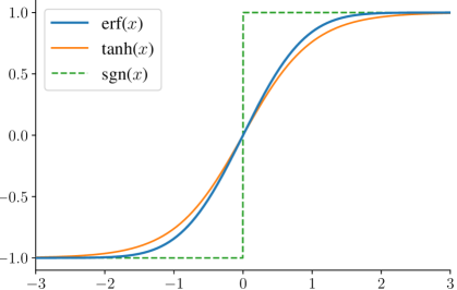
Figure 3: Visual comparison between the $\mathrm{erf}$, $\tanh$ and $\mathrm{sgn}$ activation functions.

In their discussion, Germain et al. (2009) observe that the objective in Equation (5) is similar to the one optimized by the soft-margin Support Vector Machines (Cortes and Vapnik, 1995), by roughly interpreting the hinge loss $\max(0,1-yy^{\prime})$ as a convex surrogate of the probit loss $\mathrm{erf}(-yy^{\prime})$. Likewise, Langford and Shawe-Taylor (2002) present this parameterization of the PAC-Bayes theorem as a margin bound. In the following, we develop an original approach to neural networks based on a slightly different observation: the predictor output given by Equation (4) is reminiscent of the $\tanh$ activation used in classical neural networks (see Figure 3 in the appendix for a visual comparison). Therefore, as the linear perceptron is viewed as the building block of modern multilayer neural networks, the PAC-Bayesian specialization to binary classifiers is the cornerstone of our theoretical and algorithmic framework for BAM networks.

3 The simple case of a one hidden layer network

Let us first consider a network with one hidden layer of size $d_{1}$. Hence, this network is parameterized by weights $\theta=\mathrm{vec}(\{{\mathbf{W}}_{1},{\mathbf{w}}_{2}\})$, with ${\mathbf{W}}_{1}\in\mathds{R}^{d_{1}\times d_{0}}$ and ${\mathbf{w}}_{2}\in\mathds{R}^{d_{1}}$. Given an input ${\mathbf{x}}\in\mathds{R}^{d_{0}}$, the output of the network is

$$f_{\theta}({\mathbf{x}})=\mathrm{sgn}\big{(}{\mathbf{w}}_{2}\cdot\mathrm{sgn}({\mathbf{W}}_{1}{\mathbf{x}})\big{)}\,.$$ (6)

Following Section 2, we consider an isotropic Gaussian posterior distribution centered in $\theta$, denoted $Q_{\theta}={\mathcal{N}}(\theta,I_{D})$, over the family of all networks ${\mathcal{F}}_{D}=\{f_{\tilde{\theta}}\,|\,\tilde{\theta}\in\mathds{R}^{D}\}$. Thus, the prediction of the $Q_{\theta}$-aggregate predictor is given by $F_{\theta}({\mathbf{x}})=\operatorname*{\mathbf{E}}_{\tilde{\theta}\sim Q_{\theta}}f_{\tilde{\theta}}({\mathbf{x}})$. Note that Langford and Caruana (2001); Dziugaite and Roy (2017) also consider Gaussian distributions over neural networks parameters. However, as their analysis is not specific to a particular activation function—experiments are performed with typical activation functions (sigmoid, ReLU)—the prediction relies on sampling the parameters according to the posterior. An originality of our approach is that, by studying the sign activation function, we can calculate the exact form of $F_{\theta}({\mathbf{x}})$, as detailed below.

3.1 Deterministic network

Prediction. To compute the value of $F_{\theta}({\mathbf{x}})$, we first need to decompose the probability of each $\tilde{\theta}{=}\mathrm{vec}(\{{\mathbf{V}}_{1},{\mathbf{v}}_{2}\})\,{\sim}\,Q_{\theta}$ as $Q_{\theta}(\tilde{\theta}){=}Q_{1}({\mathbf{V}}_{1})Q_{2}({\mathbf{v}}_{2})$, with $Q_{1}{=}{\mathcal{N}}({\mathbf{W}}_{1},I_{d_{0}d_{1}})$ and $Q_{2}{=}{\mathcal{N}}({\mathbf{w}}_{2},I_{d_{1}})$.

$$F_{\theta}({\mathbf{x}})= \int_{\mathds{R}^{d_{1}\times d_{0}}}Q_{1}({\mathbf{V}}_{1})\int_{\mathds{R}^{d_{1}}}Q_{2}({\mathbf{v}}_{2})\mathrm{sgn}({\mathbf{v}}_{2}\cdot\mathrm{sgn}({\mathbf{V}}_{1}{\mathbf{x}}))d{\mathbf{v}}_{2}d{\mathbf{V}}_{1}$$

$$= \int_{\mathds{R}^{d_{1}\times d_{0}}}Q_{1}({\mathbf{V}}_{1})\,\mathrm{erf}\left(\tfrac{{\mathbf{w}}_{2}\cdot\mathrm{sgn}({\mathbf{V}}_{1}{\mathbf{x}})}{\sqrt{2}\|\mathrm{sgn}({\mathbf{V}}_{1}{\mathbf{x}})\|}\right)d{\mathbf{V}}_{1}$$ (7)

$$= \sum_{{\mathbf{s}}\in\{-1,1\}^{d_{1}}}\mathrm{erf}\left(\tfrac{{\mathbf{w}}_{2}\cdot{\mathbf{s}}}{\sqrt{2d_{1}}}\right)\int_{\mathrlap{\mathds{R}^{{}_{d_{1}\times d_{0}}}}}\ \mathbb{1}[{\mathbf{s}}=\mathrm{sgn}({\mathbf{V}}_{1}{\mathbf{x}})]Q_{1}({\mathbf{V}}_{1})\,d{\mathbf{V}}_{1}$$ (8)

$$= \sum_{{\mathbf{s}}\in\{-1,1\}^{d_{1}}}\mathrm{erf}\left(\tfrac{{\mathbf{w}}_{2}\cdot{\mathbf{s}}}{\sqrt{2d_{1}}}\right)\Psi_{\mathbf{s}}\left({\mathbf{x}},{\mathbf{W}}_{1}\right),$$ (9)

where, from $Q_{1}({\mathbf{V}}_{1})=\prod_{i=1}^{d_{1}}Q_{1}^{i}({\mathbf{v}}_{1}^{i})$ with $Q_{1}^{i}\coloneqq{\mathcal{N}}({\mathbf{w}}_{1}^{i},I_{d_{0}})$, we obtain

$$\Psi_{\mathbf{s}}\left({\mathbf{x}},{\mathbf{W}}_{1}\right)\ \coloneqq\ \prod_{i=1}^{d_{1}}\int_{\mathrlap{\mathds{R}^{{}_{d_{0}}}}}\ \mathbb{1}[s_{i}\,{\mathbf{x}}\cdot{\mathbf{v}}_{1}^{i}>0]Q_{1}^{i}({\mathbf{v}}_{1}^{i})\,d{\mathbf{v}}_{1}^{i}\ =\ \prod_{i=1}^{d_{1}}\underbrace{\left[\frac{1}{2}+\frac{s_{i}}{2}\,\mathrm{erf}\!\left(\frac{{\mathbf{w}}_{1}^{i}\cdot{\mathbf{x}}}{\sqrt{2}\left\lVert{\mathbf{x}}\right\rVert}\right)\right]}_{\psi_{s_{i}}({\mathbf{x}},{\mathbf{w}}^{i}_{1})}.$$ (10)

Line (7) states that the output neuron is a linear predictor over the hidden layer’s activation values ${\mathbf{s}}=\mathrm{sgn}({\mathbf{V}}_{1}{\mathbf{x}})$; based on Equation (4), the integral on ${\mathbf{v}}_{2}$ becomes $\mathrm{erf}\big{(}{\mathbf{w}}_{2}\cdot{\mathbf{s}}/(\sqrt{2}\|{\mathbf{s}}\|)\big{)}$. As a function of ${\mathbf{s}}$, the latter expression is piecewise constant. Thus, Line (8) discretizes the integral on ${\mathbf{V}}_{1}$ as a sum of the $2^{d_{1}}$ different values of ${\mathbf{s}}=(s_{i})_{i=1}^{d_{1}},s_{i}\in\{-1,1\}$. Note that $\|{\mathbf{s}}\|^{2}=d_{1}$.

Finally, one can compute the exact output of $F_{\theta}({\mathbf{x}})$, provided one accepts to compute a sum combinatorial in the number of hidden neurons (Equation 9). We show in forthcoming Section 3.2 that it is possible to circumvent this computational burden and approximate $F_{\theta}({\mathbf{x}})$ by a sampling procedure.

Derivatives. Following contemporary approaches in deep neural networks (Goodfellow et al., 2016), we minimize the empirical loss $\widehat{\mathcal{L}}_{S}(F_{\theta})$ by stochastic gradient descent (SGD). This requires to compute the partial derivative of the cost function according to the parameters $\theta$:

$$\frac{\partial\widehat{\mathcal{L}}_{S}(F_{\theta})}{\partial\theta}=\frac{1}{n}\sum_{i=1}^{n}\frac{\partial\ell(F_{\theta}({\mathbf{x}}_{i}),y_{i})}{\partial\theta}=\frac{1}{n}\sum_{i=1}^{n}\frac{\partial F_{\theta}({\mathbf{x}}_{i})}{\partial\theta}\,\ell^{\prime}(F_{\theta}({\mathbf{x}}_{i}),y_{i})\,,$$ (11)

with the derivative of the linear loss $\ell^{\prime}(F_{\theta}({\mathbf{x}}_{i}),y_{i})=-\frac{1}{2}y$.

The partial derivatives of the prediction function (Equation 9) according to the hidden layer parameters ${\mathbf{w}}_{1}^{k}\in\{{\mathbf{w}}_{1}^{1},\ldots,{\mathbf{w}}_{1}^{d_{1}}\}$ and the output neuron parameters ${\mathbf{w}}_{2}$ are

$$\frac{\partial}{\partial{\mathbf{w}}_{1}^{k}}F_{\theta}({\mathbf{x}})= \frac{{\mathbf{x}}}{2^{\frac{3}{2}}\|{\mathbf{x}}\|}\mathrm{erf}^{\prime}\left(\frac{{\mathbf{w}}_{1}^{k}\cdot{\mathbf{x}}}{\sqrt{2}\left\lVert{\mathbf{x}}\right\rVert}\right)\sum_{{\mathbf{s}}\in\{-1,1\}^{d_{1}}}s_{k}\,\mathrm{erf}\left(\frac{{\mathbf{w}}_{2}\cdot{\mathbf{s}}}{\sqrt{2d_{1}}}\right)\left[\frac{\Psi_{\mathbf{s}}({\mathbf{x}},{\mathbf{W}}_{1})}{\psi_{s_{k}}({\mathbf{x}},{\mathbf{w}}_{1}^{k})}\right],$$ (12)

$$\frac{\partial}{\partial{\mathbf{w}}_{2}}F_{\theta}({\mathbf{x}})= \frac{1}{\sqrt{2d_{1}}}\sum_{{\mathbf{s}}\in\{-1,1\}^{d_{1}}}{\mathbf{s}}\,\mathrm{erf}^{\prime}\left(\frac{{\mathbf{w}}_{2}\cdot{\mathbf{s}}}{\sqrt{2d_{1}}}\right)\Psi_{\mathbf{s}}({\mathbf{x}},{\mathbf{W}}_{1})\,,\quad\mbox{with \ $\mathrm{erf}^{\prime}(x)\coloneqq\frac{2}{\sqrt{\pi}}e^{-x^{2}}$\,.}$$ (13)

Note that this is an exact computation. A salient fact is that even though we work on non-differentiable BAM networks, we get a structure trainable by (stochastic) gradient descent by aggregating networks.

Majority vote of learned representations. Note that $\Psi_{\mathbf{s}}$ (Equation 10) defines a distribution on ${\mathbf{s}}$. Indeed, $\sum_{\mathbf{s}}\Psi_{\mathbf{s}}({\mathbf{x}},{\mathbf{W}}_{1}){=}1$, as $\Psi_{\mathbf{s}}({\mathbf{x}},{\mathbf{W}}_{1})+\Psi_{\bar{\mathbf{s}}}({\mathbf{x}},{\mathbf{W}}_{1})=2^{-d_{1}}$ for every $\bar{\mathbf{s}}\,{=}\,{-}{\mathbf{s}}$. Thus, by Equation (9) we can interpret $F_{\theta}$ akin to a majority vote predictor, which performs a convex combination of a linear predictor outputs $F_{{\mathbf{w}}_{2}}({\mathbf{s}})\coloneqq\mathrm{erf}({\mathbf{w}}_{2}\cdot{\mathbf{s}}/\sqrt{2d_{1}})$. The vote aggregates the predictions on the $2^{d_{1}}$ possible binary representations. Thus, the algorithm does not learn the representations per se, but rather the weights $\Psi_{\mathbf{s}}({\mathbf{x}},{\mathbf{W}}_{1})$ associated to every ${\mathbf{s}}$ given an input ${\mathbf{x}}$, as illustrated by Figure 1.

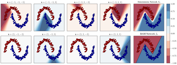
Figure 1: Illustration of the proposed method for a one hidden layer network of size $d_{1}{=}3$, interpreted as a majority vote over $8$ binary representations ${\mathbf{s}}\in\{-1,1\}^{3}$. For each ${\mathbf{s}}$, a plot shows the values of $F_{{\mathbf{w}}_{2}}({\mathbf{s}})\Psi_{\mathbf{s}}({\mathbf{x}},{\mathbf{W}}_{1})$. The sum of these values gives the deterministic network output $F_{\theta}({\mathbf{x}})$ (see Eq. 9). We also plot the BAM network output $f_{\theta}({\mathbf{x}})$ for the same parameters $\theta$ (see Eq. 6).

3.2 Stochastic approximation

Since $\Psi_{\mathbf{s}}$ (Equation 10) defines a distribution, we can interpret the function value as the probability of mapping input ${\mathbf{x}}$ into the hidden representation ${\mathbf{s}}$ given the parameters ${\mathbf{W}}_{1}$. Using a different formalism, we could write $\Pr({\mathbf{s}}|{\mathbf{x}},{\mathbf{W}}_{1})=\Psi_{\mathbf{s}}({\mathbf{x}},{\mathbf{W}}_{1})$. This viewpoint suggests a sampling scheme to approximate both the predictor output (Equation 9) and the partial derivatives (Equations 12 and 13), that can be framed as a variant of the REINFORCE algorithm (Williams, 1992) (see the discussion below): We avoid computing the $2^{d_{1}}$ terms by resorting to a Monte Carlo approximation of the sum. Given an input ${\mathbf{x}}$ and a sampling size $T$, the procedure goes as follows.

Prediction. We generate $T$ random binary vectors $Z{\coloneqq}\{{\mathbf{s}}^{t}\}_{t=1}^{T}$ according to the $\Psi_{\mathbf{s}}({\mathbf{x}},{\mathbf{W}}_{1})$-distribution. This can be done by uniformly sampling $z^{t}_{i}{\in}[0,1]$, and setting $s^{t}_{i}{=}\mathrm{sgn}(\psi_{1}({\mathbf{x}},{\mathbf{w}}_{1}^{i}){-}z^{t}_{i})$.
A stochastic approximation of $F_{\theta}({\mathbf{x}})$ is given by $\widehat{F}_{\theta}(Z)\coloneqq\frac{1}{T}\sum_{t=1}^{T}\mathrm{erf}\left(\frac{{\mathbf{w}}_{2}\cdot{\mathbf{s}}^{t}}{\sqrt{2d_{1}}}\right)$ .

Derivatives. Note that for a given sample $\{{\mathbf{s}}^{t}\}_{t=1}^{T}$, the approximate derivatives according to ${\mathbf{w}}_{2}$ (Equation 15 below) can be computed numerically by the automatic differentiation mechanism of deep learning frameworks while evaluating $\widehat{F}_{\theta}(Z)$ (e.g., Paszke et al., 2017). However, we need the following Equation (14) to approximate the gradient according to ${\mathbf{W}}_{1}$ because $\partial\widehat{F}_{\theta}(Z)/\partial{\mathbf{w}}_{1}^{k}=0$.

$$\frac{\partial}{\partial{\mathbf{w}}_{1}^{k}}F_{\theta}({\mathbf{x}}) \approx\frac{{\mathbf{x}}}{T\,2^{\frac{3}{2}}\|{\mathbf{x}}\|}\mathrm{erf}^{\prime}\left(\frac{{\mathbf{w}}_{1}^{k}\cdot{\mathbf{x}}}{\sqrt{2}\left\lVert{\mathbf{x}}\right\rVert}\right)\sum_{t=1}^{T}\frac{s^{t}_{k}}{\psi_{s^{t}_{k}}({\mathbf{x}},{\mathbf{w}}_{1}^{k})}\mathrm{erf}\left(\frac{{\mathbf{w}}_{2}\cdot{\mathbf{s}}^{t}}{\sqrt{2d_{1}}}\right);$$ (14)

$$\frac{\partial}{\partial{\mathbf{w}}_{2}}F_{\theta}({\mathbf{x}}) \approx\frac{1}{T\sqrt{2d_{1}}}\sum_{t=1}^{T}{\mathbf{s}}^{t}\,\mathrm{erf}^{\prime}\left(\frac{{\mathbf{w}}_{2}\cdot{\mathbf{s}}^{t}}{\sqrt{2d_{1}}}\right)=\frac{\partial}{\partial{\mathbf{w}}_{2}}\widehat{F}_{\theta}(Z)\,.$$ (15)

Similar approaches to stochastic networks. Random activation functions are commonly used in generative neural networks, and tools have been developed to train these by gradient descent (see Goodfellow et al. (2016, Section 20.9) for a review). Contrary to these approaches, our analysis differs as the stochastic operations are introduced to estimate a deterministic objective. That being said, Equation (14) can be interpreted as a variant of REINFORCE algorithm (Williams, 1992) to apply the back-propagation method along with discrete activation functions. Interestingly, the formulation we obtain through our PAC-Bayes objective is similar to a commonly used REINFORCE variant (e.g., Bengio et al., 2013; Yin and Zhou, 2019), where the activation function is given by a Bernoulli variable with probability of success $\sigma(a)$, where $a$ is the neuron input, and $\sigma$ is the sigma is the sigmoid function. The latter can be interpreted as a surrogate of our $\psi_{s_{i}}({\mathbf{x}},{\mathbf{w}}^{i}_{1})$.

4 Generalization to multilayer networks

In the following, we extend the strategy introduced in Section 3 to BAM architectures with an arbitrary number of layers $L\in\mathds{N}^{*}$ (Equation 1). An apparently straightforward approach to achieve this generalization would have been to consider a Gaussian posterior distribution ${\mathcal{N}}(\theta,I_{D})$ over the BAM family $\{f_{\tilde{\theta}}|\tilde{\theta}\in\mathds{R}^{D}\}$. However, doing so leads to a deterministic network relying on undesirable sums of $\prod_{k=1}^{L}2^{d_{k}}$ elements (see Appendix A.2 for details). Instead, we define a mapping $f_{\theta}\mapsto g_{\zeta(\theta)}$ which transforms the BAM network into a computation tree, as illustrated by Figure 2.

Figure 2: Illustration of the BAM to tree architecture map on a three layers network.

BAM to tree architecture map. Given a BAM network $f_{\theta}$ of $L$ layers with sizes $d_{0},d_{1},\ldots,d_{L}$ (reminder: $d_{L}{=}1$), we obtain a computation tree by decoupling the neurons (i.e., the computation graph nodes): the tree leaves contain $\prod_{k=1}^{L}d_{k}$ copies of each of the $d_{0}$ BAM input neurons, and the tree root node corresponds to the single BAM output neuron. Each input-output path of the original BAM network becomes a path of length $L$ from one leaf to the tree root. Each tree edge has its own parameter (a real-valued scalar); the total number of edges is $D^{\dagger}\coloneqq\sum_{k=0}^{L-1}d^{\dagger}_{k}$, with $d^{\dagger}_{k}\coloneqq\prod_{i=k}^{L}d_{i}$. We define a set of tree parameters $\eta$ recursively according to the tree structure. From level $k$ to $k{+}1$, the tree has $d^{\dagger}_{k}$ edges. That is, each node at level $k{+}1$ has its own parameters subtree $\eta^{k+1}\coloneqq\{\eta^{k}_{i}\}_{i=0}^{d_{k}}$, where each $\eta^{k}_{i}$ is either a weight vector containing the input edges parameters (by convention, $\eta^{k}_{0}\in\mathds{R}^{d_{k-1}}$) or a parameter set (thus, $\eta^{k}_{1},\ldots,\eta^{k}_{d_{k-1}}$ are themselves parameter subtrees). Hence, the deepest elements of the recursive parameters set $\eta$ are weight vectors $\eta^{1}\in\mathds{R}^{d_{0}}$. Let us now define the output tree $g_{\eta}({\mathbf{x}})\coloneqq g_{L}({\mathbf{x}},\eta)$ on an input ${\mathbf{x}}\in\mathds{R}^{d_{0}}$ as a recursive function:

$$g_{1}({\mathbf{x}},\{{\mathbf{w}}\}) =\mathrm{sgn}\left({\mathbf{w}}\cdot{\mathbf{x}}\right),$$

$$g_{k+1}({\mathbf{x}},\underbrace{\{{\mathbf{w}},\eta^{k}_{1},\ldots,\eta^{k}_{d_{k}}\}}_{\eta^{k}}) =\mathrm{sgn}\Big{(}{\mathbf{w}}\cdot\underbrace{(g_{k}({\mathbf{x}},\eta_{1}),\ldots,g_{k}({\mathbf{x}},\eta_{d_{k}}))}_{{\mathbf{g}}_{k}({\mathbf{x}},\eta^{k})}\Big{)}\mbox{ for $k=1,\ldots,L{-}1$}\,.$$

BAM to tree parameters map. Given BAM parameters $\theta$, we denote $\theta_{1:k}\coloneqq\mathrm{vec}\!\left(\{{\mathbf{W}}_{k}\}_{i=1}^{k}\right)$. The mapping from $\theta$ into the corresponding (recursive) tree parameters set is $\zeta(\theta)=\{{\mathbf{w}}_{L},\zeta_{1}(\theta_{1:L-1}),\ldots,\zeta_{d_{L-1}}(\theta_{1:L-1})\}$, such that $\zeta_{i}(\theta_{1:k})=\{{\mathbf{w}}_{k}^{i},\zeta_{1}(\theta_{1:k-1}),\ldots,\zeta_{d_{k-1}}(\theta_{1:k-1})\}$, and $\zeta_{i}(\theta_{1:1})=\{{\mathbf{w}}_{1}^{i}\}$. Note that the parameters tree obtained by the transformation $\zeta(\theta)$ is highly redundant, as each weight vector ${\mathbf{w}}_{k}^{i}$ (the $i$th line of the ${\mathbf{W}}_{k}$ matrix from $\theta$) is replicated $d^{\dagger}_{k+1}$ times. This construction is such that $f_{\theta}({\mathbf{x}})=g_{\zeta(\theta)}({\mathbf{x}})$ for all ${\mathbf{x}}\in\mathds{R}^{d_{0}}$.

Deterministic network. With a slight abuse of notation, we let $\tilde{\eta}\sim Q_{\eta}\coloneqq{\mathcal{N}}(\eta,I_{D^{\dagger}})$ denote a parameter tree of the same structure as $\eta$, where every weight is sampled iid from a normal distribution. We denote $G_{\theta}({\mathbf{x}})\coloneqq\operatorname*{\mathbf{E}}_{{\tilde{\eta}}\sim Q_{\zeta(\theta)}}g_{\tilde{\eta}}({\mathbf{x}})$, and we compute the output value of this predictor recursively. In the following, we denote $G^{{}_{(j)}}_{\theta_{1:k+1}}({\mathbf{x}})$ the function returning the $j$th neuron value of the layer $k{+}1$. Hence, the output of this network is $G_{\theta}({\mathbf{x}})=G^{{}_{(1)}}_{\theta_{1:L}}({\mathbf{x}})$. As such,

$$G^{(j)}_{\theta_{1:1}}({\mathbf{x}})\ = \int_{\mathds{R}^{d_{0}}}Q_{{\mathbf{w}}_{1}^{j}}({\mathbf{v}})\mathrm{sgn}({\mathbf{v}}\cdot{\mathbf{x}})d{\mathbf{v}}\ =\ \mathrm{erf}\left(\tfrac{{\mathbf{w}}_{1}^{j}\cdot{\mathbf{x}}}{\sqrt{2}\|{\mathbf{x}}\|}\right),$$

$$G^{(j)}_{\theta_{1:k+1}}({\mathbf{x}})= \sum_{\mathclap{{\mathbf{s}}\in\{-1,1\}^{d_{k}}}}\mathrm{erf}\left(\tfrac{{\mathbf{w}}_{k+1}^{j}\cdot{\mathbf{s}}}{\sqrt{2d_{k}}}\right)\Psi^{k}_{\mathbf{s}}({\mathbf{x}},\theta),\mbox{ with }\Psi^{k}_{\mathbf{s}}({\mathbf{x}},\theta)=\prod_{i=1}^{d_{k}}\,\left(\frac{1}{2}+\frac{1}{2}s_{i}\times G^{(i)}_{\theta_{1:k}}({\mathbf{x}})\right).$$ (16)

The complete mathematical calculations leading to the above results are provided in Appendix A.3. The computation tree structure and the parameter mapping $\zeta(\theta)$ are crucial to obtain the recursive expression of Equation (16). However, note that this abstract mathematical structure is never manipulated explicitly. Instead, it allows computing each hidden layer vector $(G^{{}_{(j)}}_{\theta_{1:k}}({\mathbf{x}}))_{j=1}^{d_{k}}$ sequentially; a summation of $2^{d_{k}}$ terms is required for each layer $k=1,\ldots,L{-}1$.

Stochastic approximation. Following the Section 3.2 sampling procedure trick for the one hidden layer network, we propose to perform a stochastic approximation of the network prediction output, by a Monte Carlo sampling for each layer. Likewise, we recover exact and approximate derivatives in a layer-by-layer scheme. The related equations are given in Appendix A.4.

5 PBGNet: PAC-Bayesian SGD learning of binary activated networks

We design an algorithm to learn the parameters $\theta\in\mathds{R}^{D}$ of the predictor $G_{\theta}$ by minimizing a PAC-Bayesian upper bound on the generalization loss ${\mathcal{L}}_{\mathcal{D}}(G_{\theta})$. We name our algorithm PBGNet (PAC-Bayesian Binary Gradient Network), as it is a generalization of the PBGD (PAC-Bayesian Gradient Descent) learning algorithm for linear classifiers (Germain et al., 2009) to deep binary activated neural networks.

Kullback-Leibler regularization. The computation of a PAC-Bayesian bound value relies on two key elements: the empirical loss on the training set and the Kullback-Leibler divergence between the prior and the posterior. Sections 3 and 4 present exact computation and approximation schemes for the empirical loss $\widehat{\mathcal{L}}_{S}(G_{\theta})$ (which is equal to $\widehat{\mathcal{L}}_{S}(F_{\theta})$ when $L{=}2$). Equation (17) introduces the $\mathrm{KL}$-divergence associated to the parameter maps of Section 2. We use the shortcut notation ${\mathcal{K}}(\theta,\mu)$ to refer to the divergence between two multivariate Gaussians of $D^{\dagger}$ dimensions, corresponding to learned parameters $\theta=\mathrm{vec}\!\left(\{{\mathbf{W}}_{k}\}_{k=1}^{L}\right)$ and prior parameters $\mu=\mathrm{vec}\!\left(\{{\mathbf{U}}_{k}\}_{k=1}^{L}\right)$.

$${\mathcal{K}}(\theta,\mu)\coloneqq\mathrm{KL}\Big{(}Q_{\zeta(\theta)}\,\big{\|}\,P_{\zeta(\mu)}\Big{)}=\frac{1}{2}\left(\|{\mathbf{w}}_{L}-{\mathbf{u}}_{L}\|^{2}+\sum_{k=1}^{L-1}d^{\dagger}_{k+1}\big{\|}{\mathbf{W}}_{k}-{\mathbf{U}}_{k}\big{\|}^{2}_{F}\right),$$ (17)

where the factors $d^{\dagger}_{k+1}=\prod_{i=k+1}^{L}d_{i}$ are due to the redundancy introduced by transformation $\zeta(\cdot)$. This has the effect of penalizing more the weights on the first layers. It might have a considerable influence on the bound value for very deep networks. On the other hand, we observe that this is consistent with the fine-tuning practice performed when training deep neural networks for a transfer learning task: prior parameters are learned on a first dataset, and the posterior weights are learned by adjusting the last layer weights on a second dataset (see Bengio, 2009; Yosinski et al., 2014).

Bound minimization. PBGNet minimizes the bound of Theorem 1 (rephrased as Equation 18). However, this is done indirectly by minimizing a variation on Theorem 2 and used in a deep learning context by Zhou et al. (2019) (Equation 19). Theorem 3 links both results (proof in Appendix A.5).

Theorem 3.

Given prior parameters $\mu\in\mathds{R}^{D}$, with probability at least $1-\delta$ over $S\sim{\mathcal{D}}^{n}$, we have for all $\theta$ on $\mathds{R}^{D}$ :

$${\mathcal{L}}_{\mathcal{D}}(G_{\theta})\, \leq\sup_{0\leq p\leq 1}\left\{p:\mathrm{kl}(\widehat{\mathcal{L}}_{S}(G_{\theta})\|p)\leq\frac{1}{n}[{\mathcal{K}}(\theta,\mu)+\ln\tfrac{2\sqrt{n}}{\delta}]\right\}$$ (18)

$$=\inf_{C>0}\left\{\tfrac{1}{1-e^{-C}}\left(1-\exp\left(-C\,\widehat{\mathcal{L}}_{S}(G_{\theta})-\frac{1}{n}[{\mathcal{K}}(\theta,\mu)+\ln\tfrac{2\sqrt{n}}{\delta}]\right)\right)\right\}.$$ (19)

We use stochastic gradient descent (SGD) as the optimization procedure to minimize Equation (19) with respect to $\theta$ and $C$. It optimizes the same trade-off as in Equation (5), but choosing the $C$ value which minimizes the bound. The originality of our SGD approach is that not only do we induce gradient randomness by selecting mini-batches among the training set $S$, we also approximate the loss gradient by sampling $T$ elements for the combinatorial sum at each layer. Our experiments show that, for some learning problems, reducing the sample size of the Monte Carlo approximation can be beneficial to the stochastic gradient descent. Thus the sample size value $T$ has an influence on the cost function space exploration during the training procedure (see Figure LABEL:fig:sample_effect in the appendix). Hence, we consider $T$ as a PBGNet hyperparameter.

6 Numerical experiments

Experiments were conducted on six binary classification datasets, described in Appendix B.

Learning algorithms. In order to get insights on the trade-offs promoted by the PAC-Bayes bound minimization, we compared PBGNet to variants focusing on empirical loss minimization. We train the models using multiple network architectures (depth and layer size) and hyperparameter choices. The objective is to evaluate the efficiency of our PAC-Bayesian framework both as a learning algorithm design tool and a model selection criterion. For all methods, the network parameters are trained using the Adam optimizer (Kingma and Ba, 2015). Early stopping is used to interrupt the training when the cost function value is not improved for 20 consecutive epochs. Network architectures explored range from 1 to 3 hidden layers ($L$) and a hidden size $h\in\{10,50,100\}$ ($d_{k}=h$ for $1\leq k<L$). Unless otherwise specified, the same randomly initialized parameters are used as a prior in the bound and as a starting point for SGD optimization (as in Dziugaite and Roy, 2017). Also, for all models except MLP, we select the binary activation sampling size $T$ in a range going from 10 to 10000. More details about the experimental setting are given in Appendix B.

MLP.  We compare to a standard network with $\tanh$ activation, as this activation resembles the $\mathrm{erf}$ function of PBGNet. We optimize the linear loss as the cost function and use 20% of training data as validation for hyperparameters selection. A weight decay parameter $\rho$ is selected between $0$ and $10^{-4}$. Using weight decay corresponds to adding an $L2$ regularizer $\frac{\rho}{2}\|\theta\|^{2}$ to the cost function, but contrary to the regularizer of Equation (17) promoted by PBGNet, this regularization is uniform for all layers.

PBGNet_ℓ.  This variant minimizes the empirical loss $\widehat{\mathcal{L}}(G_{\theta})$, with an $L2$ regularization term $\frac{\rho}{2}\|\theta\|^{2}$. The corresponding weight decay $\rho$, as well as other hyperparameters, are selected using a validation set, exactly as the MLP does. The bound expression is not involved in the learning process and is computed on the model selected by the validation set technique.

PBGNet${}_{\ell\text{-bnd}}$.  Again, the empirical loss $\widehat{\mathcal{L}}(G_{\theta})$ with an $L2$ regularization term $\frac{\rho}{2}\|\theta\|^{2}$ is minimized. However, only the weight decay hyperparameter $\rho$ is selected on the validation set, the other ones are selected by the bound. This method is motivated by an empirical observation: our PAC-Bayesian bound is a great model selection tool for most hyperparameters, except the weight decay term.

PBGNet.  As described in Section 5, the generalization bound is directly optimized as the cost function during the learning procedure and used solely for hyperparameters selection: no validation set is needed and all training data $S$ are exploited for learning.

PBGNet${}_{\text{pre}}$.  We also explore the possibility of using a part of the training data as a pre-training step. To do so, we split the training set into two halves. First, we minimize the empirical loss for a fixed number of 20 epochs on the first 50% of the training set. Then, we use the learned parameters as initialization and prior for PBGNet and learn on the second 50% of the training set.

Analysis. Results are summarized in Table 1, which highlights the strengths and weaknesses of the models. Both MLP and PBGNet_ℓ obtain competitive error scores but lack generalization guarantees. By introducing the bound value in the model selection process, even with the linear loss as the cost function, PBGNet${}_{\ell\text{-bnd}}$ yields non-vacuous generalization bound values although with an increase in error scores. Using the bound expression for the cost function in PBGNet improves bound values while keeping similar performances. The Ads dataset is a remarkable exception where the small amount of training examples seems to radically constrain the network in the learning process as it hinders the KL divergence growth in the bound expression. With an informative prior from pre-training, PBGNet${}_{\text{pre}}$ is able to recover competitive error scores while offering tight generalization guarantees. All selected hyperparameters are presented in the appendix (Table 4).

A notable observation is the impact of the bound exploitation for model selection on the train-test error gap. Indeed, PBGNet${}_{\ell\text{-bnd}}$, PBGNet and PBGNet${}_{\text{pre}}$ display test errors closer to their train errors, as compared to MLP and PBGNet_ℓ. This behavior is more noticeable as the dataset size grows and suggests potential robustness to overfitting when the bound is involved in the learning process.

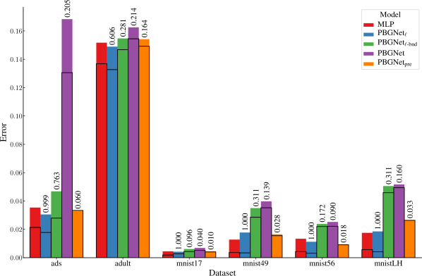
Figure 5: Visualization of experiment results for the models on the binary classification datasets. The colored bars display the test error while the black outlined bars exhibit the train error. The PAC-Bayesian bounds are identified on the top of the bars and hold with probability 0.95.

Table 1: Experiment results for the considered models on the binary classification datasets: error rates on the train and test sets (E_S and E_T), and generalization bounds on the linear loss ${\mathcal{L}}_{\mathcal{D}}$ (Bnd). The PAC-Bayesian bounds hold with probability $0.95$. Bound values for PBGNet_ℓ are trivial, excepted Adult with a bound value of 0.606, and are thus not reported. A visual representation of this table is presented in the appendix (Figure 5).

Dataset	MLP		PBGNetℓ		PBGNet${}_{\ell\text{-bnd}}$			PBGNet			PBGNet${}_{\text{pre}}$
	ES	ET	ES	ET	ES	ET	Bnd	ES	ET	Bnd	ES	ET	Bnd
ads	0.021	0.035	0.018	0.030	0.028	0.047	0.763	0.131	0.168	0.205	0.033	0.033	0.060
adult	0.137	0.152	0.133	0.149	0.147	0.155	0.281	0.154	0.163	0.214	0.149	0.154	0.164
mnist17	0.002	0.004	0.003	0.004	0.004	0.006	0.096	0.005	0.007	0.040	0.004	0.004	0.010
mnist49	0.004	0.013	0.003	0.018	0.029	0.035	0.311	0.035	0.040	0.139	0.016	0.017	0.028
mnist56	0.004	0.013	0.003	0.011	0.022	0.024	0.172	0.022	0.025	0.090	0.009	0.009	0.018
mnistLH	0.006	0.018	0.004	0.019	0.046	0.051	0.311	0.049	0.052	0.160	0.026	0.027	0.033

7 Conclusion and perspectives

We made theoretical and algorithmic contributions towards a better understanding of generalization abilities of binary activated multilayer networks, using PAC-Bayes. Note that the computational complexity of a learning epoch of PBGNet is higher than the cost induced in binary neural networks (Bengio, 2009; Hubara et al., 2016; Soudry et al., 2014; Hubara et al., 2017). Indeed, we focus on the optimization of the generalization guarantee more than computational complexity. Although we also propose a sampling scheme that considerably reduces the learning time required by our method, achieving a nontrivial tradeoff.

We intend to investigate how we could leverage the bound to learn suitable priors for PBGNet. Or equivalently, finding (from the bound point of view) the best network architecture. We also plan to extend our analysis to multiclass and multilabel prediction, and convolutional networks. We believe that this line of work is part of a necessary effort to give rise to a better understanding of the behavior of deep neural networks.

Acknowledgments

We would like to thank Mario Marchand for the insight leading to the Theorem 3, Gabriel Dubé and Jean-Samuel Leboeuf for their input on the theoretical aspects, Frédérik Paradis for his help with the implementation, and Robert Gower for his insightful comments. This work was supported in part by the French Project APRIORI ANR-18-CE23-0015, in part by NSERC and in part by Intact Financial Corporation. We gratefully acknowledge the support of NVIDIA Corporation with the donation of Titan Xp GPUs used for this research.

Appendix A Supplementary Material

A.1 From the sign activation to the erf function

For completeness, we present the detailed derivation of Equation (4). This result appears namely in Langford and Shawe-Taylor [2002], Langford [2005], Germain et al. [2009].

Given ${\mathbf{x}}\in\mathds{R}^{d}$, we have

$$F_{\mathbf{w}}({\mathbf{x}}) =\operatorname*{\mathbf{E}}_{{\mathbf{v}}\sim{\mathcal{N}}({\mathbf{w}},\mathrm{I})}\mathrm{sgn}({\mathbf{v}}\cdot{\mathbf{x}})$$

$$=\int_{\mathds{R}^{d}}\mathrm{sgn}({\mathbf{v}}\cdot{\mathbf{x}})\left(\frac{1}{\sqrt{2\pi}}\right)^{d}e^{-\frac{1}{2}\left\lVert{\mathbf{v}}-{\mathbf{w}}\right\rVert^{2}}d{\mathbf{v}}$$

$$=\int_{\mathds{R}^{d}}\left(\mathbb{1}\left[{\mathbf{v}}\cdot{\mathbf{x}}>0\right]-\mathbb{1}\left[{\mathbf{v}}\cdot{\mathbf{x}}<0\right]\right)\left(\frac{1}{\sqrt{2\pi}}\right)^{d}e^{-\frac{1}{2}\left\lVert{\mathbf{v}}-{\mathbf{w}}\right\rVert^{2}}d{\mathbf{v}}$$

$$=\left(\frac{1}{\sqrt{2\pi}}\right)^{d}\int_{\mathds{R}^{d}}\mathbb{1}\left[{\mathbf{v}}\cdot{\mathbf{x}}>0\right]e^{-\frac{1}{2}\left\lVert{\mathbf{v}}-{\mathbf{w}}\right\rVert^{2}}d{\mathbf{v}}-\left(\frac{1}{\sqrt{2\pi}}\right)^{d}\int_{\mathds{R}^{d}}\mathbb{1}\left[{\mathbf{v}}\cdot{\mathbf{x}}<0\right]e^{-\frac{1}{2}\left\lVert{\mathbf{v}}-{\mathbf{w}}\right\rVert^{2}}d{\mathbf{v}}\,.$$

Without loss of generality, let us consider a vector basis where $\frac{{\mathbf{x}}}{\left\lVert{\mathbf{x}}\right\rVert}$ is the first coordinate. In this basis, the first elements of the vectors ${\mathbf{v}}=(v_{1},v_{2},\dots,v_{d})$ and ${\mathbf{w}}=(w_{1},w_{2},\dots,w_{d})$ are

$$v_{1}=\frac{{\mathbf{v}}\cdot{\mathbf{x}}}{\left\lVert{\mathbf{x}}\right\rVert}, w_{1}=\frac{{\mathbf{w}}\cdot{\mathbf{x}}}{\left\lVert{\mathbf{x}}\right\rVert}\,.$$

Hence, ${\mathbf{v}}\cdot{\mathbf{x}}=v_{1}\cdot\left\lVert{\mathbf{x}}\right\rVert$ with $\left\lVert{\mathbf{x}}\right\rVert>0$. Looking at the left side of the subtraction from the previous equation, we thus have

$$\left(\frac{1}{\sqrt{2\pi}}\right)^{d}\int_{\mathds{R}^{d}} \mathbb{1}\left[{\mathbf{v}}\cdot{\mathbf{x}}>0\right]e^{-\frac{1}{2}\left\lVert{\mathbf{v}}-{\mathbf{w}}\right\rVert^{2}}d{\mathbf{v}}$$

$$=\int_{\mathds{R}}\mathbb{1}\left[v_{1}>0\right]\frac{1}{\sqrt{2\pi}}e^{-\frac{1}{2}(v_{1}-w_{1})^{2}}\left[\int_{\mathds{R}^{d-1}}\left(\frac{1}{\sqrt{2\pi}}\right)^{d-1}e^{-\frac{1}{2}\left\lVert{\mathbf{v}}_{2:d}-{\mathbf{w}}_{2:d}\right\rVert^{2}}d{\mathbf{v}}_{2:d}\right]dv_{1}$$

$$=\frac{1}{\sqrt{2\pi}}\int_{-\infty}^{\infty}\mathbb{1}\left[t>-w_{1}\right]e^{-\frac{1}{2}t^{2}}dt\,,$$

with $t\coloneqq v_{1}-w_{1}$. Hence,

$$\operatorname*{\mathbf{E}}_{{\mathbf{v}}\sim{\mathcal{N}}({\mathbf{w}},\mathrm{I})}\mathrm{sgn}({\mathbf{v}}\cdot{\mathbf{x}}) =\frac{1}{\sqrt{2\pi}}\int_{-\infty}^{\infty}\mathbb{1}\left[t>-w_{1}\right]e^{-\frac{1}{2}t^{2}}dt-\frac{1}{\sqrt{2\pi}}\int_{-\infty}^{\infty}\mathbb{1}\left[t<-w_{1}\right]e^{-\frac{1}{2}t^{2}}dt$$

$$=\frac{1}{\sqrt{2\pi}}\int_{-w_{1}}^{\infty}e^{-\frac{1}{2}t^{2}}dt-\frac{1}{\sqrt{2\pi}}\int_{-\infty}^{-w_{1}}e^{-\frac{1}{2}t^{2}}dt$$

$$=\frac{1}{2}+\frac{1}{\sqrt{2\pi}}\int_{0}^{w_{1}}e^{-\frac{1}{2}t^{2}}dt-\frac{1}{2}+\frac{1}{\sqrt{2\pi}}\int_{0}^{w_{1}}e^{-\frac{1}{2}t^{2}}dt$$

$$=\frac{\sqrt{2}}{\sqrt{\pi}}\int_{0}^{w_{1}}e^{-\frac{1}{2}t^{2}}dt$$

$$=\frac{2}{\sqrt{\pi}}\int_{0}^{\frac{w_{1}}{\sqrt{2}}}e^{-u^{2}}du\quad\mbox{ with }u=\tfrac{t}{\sqrt{2}}$$

$$=\mathrm{erf}\left(\frac{w_{1}}{\sqrt{2}}\right)$$

$$=\mathrm{erf}\left(\frac{{\mathbf{w}}\cdot{\mathbf{x}}}{\sqrt{2}\left\lVert{\mathbf{x}}\right\rVert}\right),$$

where $\mathrm{erf}(\cdot)$ is the Gauss error function defined as $\mathrm{erf}(x)=\frac{2}{\sqrt{\pi}}\int_{0}^{x}e^{-t^{2}}dt$.

A.2 Aggregation of multilayer networks without the tree architecture

To understand the benefit of the BAM to tree architecture map introduced in Section 4, let us compute the prediction function of an aggregation of two hidden layers networks following the same strategy as for the single hidden layer case (see Subsection 3.1).

The two hidden layer network is parameterized by weights $\theta=\mathrm{vec}(\{{\mathbf{W}}_{1},{\mathbf{W}}_{2},{\mathbf{w}}_{3}\})$, with ${\mathbf{W}}_{1}\in\mathds{R}^{d_{1}\times d_{0}}$, ${\mathbf{W}}_{2}\in\mathds{R}^{d_{2}\times d_{1}}$ and ${\mathbf{w}}_{3}\in\mathds{R}^{d_{2}}$. Given an input ${\mathbf{x}}\in\mathds{R}^{d_{0}}$, the output of the network is

$$f_{\theta}({\mathbf{x}})=\mathrm{sgn}\big{(}{\mathbf{w}}_{3}\cdot\mathrm{sgn}({\mathbf{W}}_{2}\cdot\mathrm{sgn}({\mathbf{W}}_{1}{\mathbf{x}}))\big{)}\,.$$ (20)

We seek to compute $F_{\theta}({\mathbf{x}})=\operatorname*{\mathbf{E}}_{\tilde{\theta}\sim Q_{\theta}}f_{\tilde{\theta}}({\mathbf{x}})$ with $\tilde{\theta}=\mathrm{vec}(\{{\mathbf{V}}_{1},{\mathbf{V}}_{2},{\mathbf{v}}_{3}\})$ and $Q_{\theta}={\mathcal{N}}(\theta,I_{D})$. First, we need to decompose the probability of each $\tilde{\theta}\sim Q_{\theta}$ as $Q_{\theta}(\tilde{\theta}){=}Q_{1}({\mathbf{V}}_{1})Q_{2}({\mathbf{V}}_{2})Q_{3}({\mathbf{v}}_{3})$, with $Q_{1}{=}{\mathcal{N}}({\mathbf{W}}_{1},I_{d_{0}d_{1}})$, $Q_{2}{=}{\mathcal{N}}({\mathbf{W}}_{2},I_{d_{1}d_{2}})$ and $Q_{3}{=}{\mathcal{N}}({\mathbf{w}}_{3},I_{d_{2}})$.

$$F_{\theta}({\mathbf{x}})= \operatorname*{\mathbf{E}}_{\tilde{\theta}\sim Q_{\theta}}f_{\tilde{\theta}}({\mathbf{x}})$$

$$= \int_{\mathrlap{\mathds{R}^{d_{1}\times d_{0}}}}\ Q_{1}({\mathbf{V}}_{1})\int_{\mathrlap{\mathds{R}^{d_{2}\times d_{1}}}}\ Q_{2}({\mathbf{V}}_{2})\int_{\mathrlap{\mathds{R}^{d_{2}}}}\ Q_{3}({\mathbf{v}}_{3})\mathrm{sgn}({\mathbf{v}}_{3}\cdot\mathrm{sgn}({\mathbf{V}}_{2}\mathrm{sgn}({\mathbf{V}}_{1}{\mathbf{x}})))d{\mathbf{v}}_{3}d{\mathbf{V}}2d{\mathbf{V}}_{1}$$

$$= \int_{\mathrlap{\mathds{R}^{d_{1}\times d_{0}}}}\ Q_{1}({\mathbf{V}}_{1})\int_{\mathrlap{\mathds{R}^{d_{2}\times d_{1}}}}\ Q_{2}({\mathbf{V}}_{2})\,\mathrm{erf}\left(\tfrac{{\mathbf{w}}_{3}\cdot\mathrm{sgn}({\mathbf{V}}_{2}\mathrm{sgn}({\mathbf{V}}_{1}{\mathbf{x}}))}{\sqrt{2}\|\mathrm{sgn}({\mathbf{V}}_{2}\mathrm{sgn}({\mathbf{V}}_{1}{\mathbf{x}}))\|}\right)d{\mathbf{V}}_{2}d{\mathbf{V}}_{1}$$

$$= \sum_{\mathclap{{\mathbf{t}}\in\{-1,1\}^{d_{2}}}}\mathrm{erf}\left(\tfrac{{\mathbf{w}}_{3}\cdot{\mathbf{t}}}{\sqrt{2d_{2}}}\right)\int_{\mathrlap{\mathds{R}^{d_{1}\times d_{0}}}}\ Q_{1}({\mathbf{V}}_{1})\int_{\mathrlap{\mathds{R}^{d_{2}\times d_{1}}}}\ Q_{2}({\mathbf{V}}_{2})\ \mathbb{1}[{\mathbf{t}}=\mathrm{sgn}({\mathbf{V}}_{2}\mathrm{sgn}({\mathbf{V}}_{1}{\mathbf{x}}))]\,d{\mathbf{V}}_{2}d{\mathbf{V}}_{1}$$

$$= \sum_{\mathclap{{\mathbf{t}}\in\{-1,1\}^{d_{2}}}}\mathrm{erf}\left(\tfrac{{\mathbf{w}}_{3}\cdot{\mathbf{t}}}{\sqrt{2d_{2}}}\right)\int_{\mathrlap{\mathds{R}^{d_{1}\times d_{0}}}}\ Q_{1}({\mathbf{V}}_{1})\prod_{i=1}^{d_{2}}\int_{\mathrlap{\mathds{R}^{d_{2}\times d_{1}}}}\ Q_{2}^{i}({\mathbf{v}}_{2}^{i})\ \mathbb{1}[t_{i}\mathrm{sgn}({\mathbf{v}}_{2}^{i}\mathrm{sgn}({\mathbf{V}}_{1}{\mathbf{x}}))>0]\,d{\mathbf{v}}_{2}^{i}d{\mathbf{V}}_{1}$$

$$= \sum_{\mathclap{{\mathbf{t}}\in\{-1,1\}^{d_{2}}}}\mathrm{erf}\left(\tfrac{{\mathbf{w}}_{3}\cdot{\mathbf{t}}}{\sqrt{2d_{2}}}\right)\sum_{\mathclap{{\mathbf{s}}\in\{-1,1\}^{d_{1}}}}\quad\,\,\,\int_{\mathrlap{\mathds{R}^{d_{1}\times d_{0}}}}\ Q_{1}({\mathbf{V}}_{1})\mathbb{1}[{\mathbf{s}}=\mathrm{sgn}({\mathbf{V}}_{1}{\mathbf{x}})]d{\mathbf{V}}_{1}\prod_{i=1}^{d_{2}}\left[\frac{1}{2}+\frac{t_{i}}{2}\,\mathrm{erf}\!\left(\frac{{\mathbf{w}}_{2}^{i}\cdot{\mathbf{s}}}{\sqrt{2d_{1}}}\right)\right]$$

$$= \sum_{\mathclap{{\mathbf{t}}\in\{-1,1\}^{d_{2}}}}\mathrm{erf}\left(\tfrac{{\mathbf{w}}_{3}\cdot{\mathbf{t}}}{\sqrt{2d_{2}}}\right)\sum_{\mathclap{{\mathbf{s}}\in\{-1,1\}^{d_{1}}}}\quad\,\,\,\underbrace{\prod_{j=1}^{d_{1}}\left[\frac{1}{2}+\frac{s_{j}}{2}\,\mathrm{erf}\!\left(\frac{{\mathbf{w}}_{1}^{j}\cdot{\mathbf{x}}}{\sqrt{2}\left\lVert{\mathbf{x}}\right\rVert}\right)\right]}_{\Psi_{{\mathbf{s}}}({\mathbf{x}},{\mathbf{W}}_{1})}\underbrace{\prod_{i=1}^{d_{2}}\left[\frac{1}{2}+\frac{t_{i}}{2}\,\mathrm{erf}\!\left(\frac{{\mathbf{w}}_{2}^{i}\cdot{\mathbf{s}}}{\sqrt{2d_{1}}}\right)\right]}_{\Psi_{{\mathbf{t}}}({\mathbf{s}},{\mathbf{W}}_{2})}$$

For each combination of first layer activation values ${\mathbf{s}}\in\{-1,1\}^{d_{1}}$ and second layer activation values ${\mathbf{t}}\in\{-1,1\}^{d_{2}}$, one needs to compute its probability $\Psi_{{\mathbf{s}}}({\mathbf{x}},{\mathbf{W}}_{1})\Psi_{{\mathbf{t}}}({\mathbf{s}},{\mathbf{W}}_{2})$. This leads to a summation of $2^{d_{1}}\times 2^{d_{2}}$ terms. Instead, the layer by layer computation obtained by our tree mapping trick implies $2^{d_{1}}+2^{d_{2}}$ terms. This strategy enables a forward computation similar to traditional neural network, as each hidden layer values relies solely on the values of the previous layer.

A.3 Prediction for the multilayer case (with the proposed tree architecture map)

Details of the complete mathematical calculations leading to Equation (16) are presented below:

$$G^{(j)}_{\theta_{1:k+1}}({\mathbf{x}})\coloneqq \int Q_{\zeta_{j}(\theta_{1:k+1})}({\tilde{\eta}})\,g_{k+1}({\mathbf{x}},{\tilde{\eta}})\,d{\tilde{\eta}}$$

$$= \int Q_{\zeta(\theta_{1:k})}({\tilde{\eta}}_{1})\ldots\int Q_{\zeta(\theta_{1:k})}({\tilde{\eta}}_{d_{k}})\left(\int_{\mathds{R}^{d^{k}}}Q_{{\mathbf{w}}_{k}^{j}}({\mathbf{v}})\mathrm{sgn}[{\mathbf{v}}\cdot{\mathbf{g}}_{k}({\mathbf{x}},{\tilde{\eta}})]d{\mathbf{v}}\right)d{\tilde{\eta}}_{d_{k}}\dots d{\tilde{\eta}}_{1}$$

$$= \int Q_{\zeta(\theta_{1:k})}({\tilde{\eta}}_{1})\ldots\int Q_{\zeta(\theta_{1:k})}({\tilde{\eta}}_{d_{k}})\,\mathrm{erf}\left(\frac{{\mathbf{w}}_{k+1}^{j}\cdot{\mathbf{g}}_{k}({\mathbf{x}},{\tilde{\eta}})}{\sqrt{2}\|{\mathbf{g}}_{k}({\mathbf{x}},{\tilde{\eta}})\|}\right)d{\tilde{\eta}}_{d_{k}}\dots d{\tilde{\eta}}_{1}$$

$$= \sum_{\mathclap{{\mathbf{s}}\in\{-1,1\}^{d_{k}}}}\mathrm{erf}\left(\frac{{\mathbf{w}}_{k+1}^{j}\cdot{\mathbf{s}}}{\sqrt{2d_{k}}}\right)\int Q_{\zeta(\theta_{1:k})}({\tilde{\eta}}_{1})\ldots\int Q_{\zeta(\theta_{1:k})}({\tilde{\eta}}_{d_{k}})\,\mathbb{1}[{\mathbf{s}}={\mathbf{g}}_{k}({\mathbf{x}},{\tilde{\eta}})]d{\tilde{\eta}}_{d_{k}}\cdots d{\tilde{\eta}}_{1}$$

$$= \sum_{\mathclap{{\mathbf{s}}\in\{-1,1\}^{d_{k}}}}\mathrm{erf}\left(\frac{{\mathbf{w}}_{k+1}^{j}\cdot{\mathbf{s}}}{\sqrt{2d_{k}}}\right)\prod_{i=1}^{d_{k}}\int Q_{\zeta(\theta_{1:k})}({\tilde{\eta}}_{i})\,\mathbb{1}[s_{i}=g_{k}({\mathbf{x}},{\tilde{\eta}}_{i})]d{\tilde{\eta}}_{i}$$

$$= \sum_{\mathclap{{\mathbf{s}}\in\{-1,1\}^{d_{k}}}}\mathrm{erf}\left(\frac{{\mathbf{w}}^{j}_{k+1}\cdot{\mathbf{s}}}{\sqrt{2d_{k}}}\right)\prod_{i=1}^{d_{k}}\int Q_{\zeta(\theta_{1:k})}({\tilde{\eta}}_{i})\,\left(\frac{1}{2}+\frac{s_{i}}{2}g_{k}({\mathbf{x}},{\tilde{\eta}}_{i})\right)d{\tilde{\eta}}_{i}$$

$$= \sum_{\mathclap{{\mathbf{s}}\in\{-1,1\}^{d_{k}}}}\mathrm{erf}\left(\frac{{\mathbf{w}}^{j}_{k+1}\cdot{\mathbf{s}}}{\sqrt{2d_{k}}}\right)\prod_{i=1}^{d_{k}}\,\left(\frac{1}{2}+\frac{s_{i}}{2}\int Q_{\zeta(\theta_{1:k})}({\tilde{\eta}}_{i})g_{k}({\mathbf{x}},{\tilde{\eta}}_{i})d{\tilde{\eta}}_{i}\right)$$

$$= \sum_{\mathclap{{\mathbf{s}}\in\{-1,1\}^{d_{k}}}}\mathrm{erf}\left(\frac{{\mathbf{w}}^{j}_{k+1}\cdot{\mathbf{s}}}{\sqrt{2d_{k}}}\right)\underbrace{\prod_{i=1}^{d_{k}}\,\left(\frac{1}{2}+\frac{1}{2}s_{i}\times G^{(i)}_{\theta_{1:k}}({\mathbf{x}})\right)}_{\Psi^{k}_{\mathbf{s}}({\mathbf{x}},\eta)}.$$

Moreover,

$$\Psi^{k}_{\mathbf{s}}({\mathbf{x}},\theta)=\prod_{i=1}^{d_{k}}\underbrace{\,\left(\frac{1}{2}+\frac{1}{2}s_{i}\times G^{(i)}_{\theta_{1:k}}({\mathbf{x}})\right)}_{\psi^{k}_{s_{i}}({\mathbf{x}},\theta)}\,.$$

Base case:

$$G^{(j)}_{\theta_{1:1}}({\mathbf{x}}) =\operatorname*{\mathbf{E}}_{{\tilde{\eta}}\sim{\mathcal{N}}(\zeta_{j}(\theta_{1:1}),I)}g_{1}({\mathbf{x}},{\tilde{\eta}})$$

$$=\int_{\mathds{R}^{d_{0}}}Q_{{\mathbf{w}}_{1}^{j}}({\mathbf{v}})\mathrm{sgn}({\mathbf{v}}\cdot{\mathbf{x}})d{\mathbf{v}}$$

$$=\mathrm{erf}\left(\frac{{\mathbf{w}}_{1}^{j}\cdot{\mathbf{x}}}{\sqrt{2}\|{\mathbf{x}}\|}\right).$$

A.4 Derivatives of the multilayer case (with the proposed tree architecture map)

We first aim at computing $\frac{\partial}{\partial{\mathbf{w}}_{k+1}}G_{\theta_{1:k+1}}({\mathbf{x}})$.

Recall that ${\mathbf{w}}_{k}^{j}\in\{{\mathbf{w}}_{k}^{1},\ldots,{\mathbf{w}}_{k}^{d_{k}}\}$ is the $j^{\rm th}$ line of ${\mathbf{W}}_{k}$, that is the input weights of the corresponding hidden layer’s neuron.

$$\frac{\partial}{\partial{\mathbf{w}}_{k+1}^{j}}G^{(j)}_{\theta_{1:k+1}}({\mathbf{x}})= \frac{\partial}{\partial{\mathbf{w}}_{k+1}^{j}}\quad\,\,\sum_{\mathclap{{\mathbf{s}}\in\{-1,1\}^{d_{k}}}}\mathrm{erf}\left(\tfrac{{\mathbf{w}}_{k+1}^{j}\cdot{\mathbf{s}}}{\sqrt{2d_{k}}}\right)\Psi^{k}_{\mathbf{s}}({\mathbf{x}},\theta)$$

$$= \sum_{\mathclap{{\mathbf{s}}\in\{-1,1\}^{d_{k}}}}\quad\frac{{\mathbf{s}}}{\sqrt{2d_{k}}}\mathrm{erf}^{\prime}\left(\tfrac{{\mathbf{w}}_{k+1}^{j}\cdot{\mathbf{s}}}{\sqrt{2d_{k}}}\right)\Psi^{k}_{\mathbf{s}}({\mathbf{x}},\theta)\,.$$

The base case of the recursion is

$$\frac{\partial}{\partial{\mathbf{w}}_{1}^{j}}G^{(j)}_{\theta_{1:1}}({\mathbf{x}})= \frac{\partial}{\partial{\mathbf{w}}_{1}^{j}}\mathrm{erf}\left(\frac{{\mathbf{w}}_{1}^{j}\cdot{\mathbf{x}}}{\sqrt{2}\|{\mathbf{x}}\|}\right)$$

$$= \frac{{\mathbf{x}}}{\sqrt{2}\|{\mathbf{x}}\|}\mathrm{erf}^{\prime}\left(\frac{{\mathbf{w}}_{1}^{j}\cdot{\mathbf{x}}}{\sqrt{2}\|{\mathbf{x}}\|}\right).$$

In order to propagate the error through the layers, we also need to compute for $k>1$:

$$\frac{\partial}{\partial G^{(l)}_{\theta_{1:k}}}G^{(j)}_{\theta_{1:k+1}}= \frac{\partial}{\partial G^{(l)}_{\theta_{1:k}}}\quad\,\,\sum_{\mathclap{{\mathbf{s}}\in\{-1,1\}^{d_{k}}}}\mathrm{erf}\left(\frac{{\mathbf{w}}^{j}_{k+1}\cdot{\mathbf{s}}}{\sqrt{2d_{k}}}\right)\prod_{i=1}^{d_{k}}\,\left(\frac{1}{2}+\frac{1}{2}s_{i}\times G^{(i)}_{\theta_{1:k}}\right)$$

$$= \sum_{\mathclap{{\mathbf{s}}\in\{-1,1\}^{d_{k}}}}\mathrm{erf}\left(\frac{{\mathbf{w}}^{j}_{k+1}\cdot{\mathbf{s}}}{\sqrt{2d_{k}}}\right)\left[\frac{\Psi_{\mathbf{s}}^{k}({\mathbf{x}},\theta)}{\psi^{k}_{s_{l}}({\mathbf{x}},\theta)}\right]\frac{\partial}{\partial G^{(l)}_{\theta_{1:k}}}\psi^{k}_{s_{l}}({\mathbf{x}},\theta)$$

$$= \sum_{\mathclap{{\mathbf{s}}\in\{-1,1\}^{d_{k}}}}\mathrm{erf}\left(\frac{{\mathbf{w}}^{j}_{k+1}\cdot{\mathbf{s}}}{\sqrt{2d_{k}}}\right)\left[\frac{s_{l}\Psi_{\mathbf{s}}^{k}({\mathbf{x}},\theta)}{2\psi^{k}_{s_{l}}({\mathbf{x}},\theta)}\right].$$

Thus, we can compute

$$\frac{\partial\widehat{\mathcal{L}}_{S}\left(G^{(j)}_{\theta_{1:k+1}}({\mathbf{x}})\right)}{\partial{\mathbf{w}}_{k}^{j}}=\sum_{l}\frac{\partial\widehat{\mathcal{L}}_{S}\left(G^{(j)}_{\theta_{1:k+1}}({\mathbf{x}})\right)}{\partial G^{(l)}_{\theta_{1:k+1}}}\frac{\partial G^{(l)}_{\theta_{1:k+1}}}{\partial G^{(j)}_{\theta_{1:k}}}\frac{\partial G^{(j)}_{\theta_{1:k}}}{\partial{\mathbf{w}}_{k}^{j}}\,.$$

A.5 Proof of Theorem 3

Lemma 4 (Germain et al. [2009], Proposition 2.1; Lacasse [2010], Proposition 6.2.2).

For any $0\leq q\leq p<1$, we have

$$\sup_{C>0}\Big{[}\Delta(C,q,p)\Big{]}=\mathrm{kl}(q\|p)\,,$$

with

$$\Delta(C,q,p)\,\coloneqq\,-\ln(1-p(1-e^{-C}))-Cq\,.$$ (21)

Proof.

For $0\leq q,p<1$, $\Delta(C,q,p)$ is concave in $C$ and the maximum is $c_{0}=-\ln\left(\frac{qp-p}{qp-q}\right)$. Moreover, $\Delta(c_{0},q,p)=\mathrm{kl}(q\|p)$. ∎

Theorem 3. Given prior parameters $\mu\in\mathds{R}^{D}$, with probability at least $1-\delta$ over $S\sim{\mathcal{D}}^{n}$, we have for all $\theta$ on $\mathds{R}^{D}$ :

$${\mathcal{L}}_{\mathcal{D}}(G_{\theta})\, \leq\sup_{0\leq p\leq 1}\left\{p:\mathrm{kl}(\widehat{\mathcal{L}}_{S}(G_{\theta})\|p)\leq\frac{1}{n}[{\mathcal{K}}(\theta,\mu)+\ln\tfrac{2\sqrt{n}}{\delta}]\right\}$$

$$=\inf_{C>0}\left\{\tfrac{1}{1-e^{-C}}\left(1-\exp\left(-C\,\widehat{\mathcal{L}}_{S}(G_{\theta})-\frac{1}{n}[{\mathcal{K}}(\theta,\mu)+\ln\tfrac{2\sqrt{n}}{\delta}]\right)\right)\right\}.$$

Proof.

In the following, we denote $\xi\coloneqq\frac{1}{n}[{\mathcal{K}}(\theta,\mu)+\ln\tfrac{2\sqrt{n}}{\delta}]$ and we assume $0<\xi<\infty$. Let us define

$$p^{*}\coloneqq\sup_{0\leq p\leq 1}\left\{p:\mathrm{kl}(\widehat{\mathcal{L}}_{S}(G_{\theta})\|p)\leq\xi\right\}.$$ (22)

First, by a straightforward rewriting of Theorem 1 [Seeger, 2002], we have, with probability at least $1-\delta$ over $S\sim{\mathcal{D}}^{n}$,

$${\mathcal{L}}_{\mathcal{D}}(G_{\theta})\leq p^{*}\,.$$

Then, we want to show

$$p^{*}=\inf_{C>0}\left\{\tfrac{1}{1-e^{-C}}\left(1-\exp\left(-C\,\widehat{\mathcal{L}}_{S}(G_{\theta})-\xi\right)\right)\right\}.$$ (23)

Case $\widehat{\mathcal{L}}_{S}(G_{\theta})<1$: The function $\mathrm{kl}(\widehat{\mathcal{L}}_{S}(G_{\theta})\|p)$ is strictly increasing for $p>\widehat{\mathcal{L}}_{S}(G_{\theta})$. Thus, the supremum value $p^{*}$ is always reached in Equation (22), so we have

$$\mathrm{kl}(\widehat{\mathcal{L}}_{S}(G_{\theta})\|p^{*})=\xi,$$

and, by Lemma 4,

$$\sup_{C>0}\Big{[}\Delta(C,\widehat{\mathcal{L}}_{S}(G_{\theta}),p^{*})\Big{]} =\xi\,,$$ (24)

$$\mbox{ and }\forall C>0:\Delta(C,\widehat{\mathcal{L}}_{S}(G_{\theta}),p^{*}) \leq\xi\,.$$ (25)

Let $C^{*}\coloneqq\operatorname*{\mathrm{argsup}}_{C>0}\Big{[}\Delta(C,\widehat{\mathcal{L}}_{S}(G_{\theta}),p^{*})\Big{]}$.

By rearranging the terms of $\Delta(C^{*},\widehat{\mathcal{L}}_{S}(G_{\theta}),p^{*})$ (see Equation 21), we obtain, from Line (24),

$$p^{*}=\tfrac{1}{1-e^{-C^{*}}}\left(1-\exp\left(-C^{*}\,\widehat{\mathcal{L}}_{S}(G_{\theta})-\xi\right)\right),$$ (26)

and, from Line (25),

$$\forall C>0:p^{*}\leq\tfrac{1}{1-e^{-C}}\left(1-\exp\left(-C\,\widehat{\mathcal{L}}_{S}(G_{\theta})-\xi\right)\right).$$ (27)

Thus, combining Lines (26) and  (27), we finally prove the desired result of Equation (23).

Case $\widehat{\mathcal{L}}_{S}(G_{\theta})=1$: From Equation (22), we have $p^{*}=1$, because $\lim_{p\to 1}\mathrm{kl}(1\|p)=0$. We also have $\frac{1-e^{-C-\xi}}{1-e^{-C}}\geq 1$ and $\lim_{C\to\infty}\left[\frac{1-e^{-C-\xi}}{1-e^{-C}}\right]=1$, thus fulfilling Equation (23). ∎

Appendix B Experiments

B.1 Datasets

In Section 6 we use the datasets Ads (a small dataset related to advertisements on web pages), Adult (a low-dimensional task about predicting income from census data) and four binary variants of the MNIST handwritten digits:

ads

http://archive.ics.uci.edu/ml/datasets/Internet+Advertisements
The first 4 features which have missing values are removed.

adult

https://archive.ics.uci.edu/ml/datasets/Adult

mnist

http://yann.lecun.com/exdb/mnist/
Binary classification tasks are compiled with the following pairs:

• Digits pairs 1 vs. 7, 4 vs. 9 and 5 vs. 6.

• Low digits vs. high digits $(\{0,1,2,3,4\}$ vs $\{5,6,7,8,9\})$ identified as mnistLH.

We split the datasets into training and testing sets with a 75/25 ratio. Table 2 presents an overview of the datasets statistics.

Table 2: Datasets overview.

Dataset	$n_{\rm train}$	$n_{\rm test}$	$d$
ads	2459	820	1554
adult	36631	12211	108
mnist17	11377	3793	784
mnist49	10336	3446	784
mnist56	9891	3298	784
mnistLH	52500	17500	784

B.2 Learning algorithms details

Table 3 summarizes the characteristics of the learning algorithms used in the experiments.

Table 3: Models overview.

Model name	Cost function	Train split	Valid split	Model selection	Prior
MLP	linear loss, L2 regularized	80%	20%	valid linear loss	-
PBGNetℓ	linear loss, L2 regularized	80%	20%	valid linear loss	random init
PBGNet${}_{\ell\text{-bnd}}$	linear loss, L2 regularized	80%	20%	hybrid (see B.2)	random init
PBGNet	PAC-Bayes bound	100 %	-	PAC-Bayes bound	random init
PBGNet${}_{\text{pre}}$
– pretrain	linear loss ($20$ epochs)	50%	-	-	random init
– final	PAC-Bayes bound	50%	-	PAC-Bayes bound	pretrain

Cost functions.

MLP, PBGNet_ℓ, PBGNet${}_{\ell\text{-bnd}}$ : The gradient descent minimizes the following according to parameters $\theta$.

$$\widehat{\mathcal{L}}_{S}(G_{\theta})+\frac{\rho}{2}\|\theta\|^{2}\,,$$

where $\rho$ is the L2 regularization “weight decay” penalization term.

PBGNet, PBGNet${}_{\text{pre}}$ : The gradient descent minimizes the following according to parameters $\theta$ and $C\in\mathds{R}^{+}$.

$$\frac{1}{1-e^{-C}}\left(1-\exp\left(-C\,\widehat{\mathcal{L}}_{S}(G_{\theta})-\frac{1}{n}\left[{\mathcal{K}}(\theta,\mu)+\ln\tfrac{2\sqrt{n}}{\delta}\right]\right)\right),$$

where ${\mathcal{K}}(\theta,\mu)$ is given by Equation (17).

Hyperparameter choices.

We execute each learning algorithm for combination of hyperparameters selected among the following values.

• Hidden layers $\in\{1,2,3\}$ .

• Hidden size $\in\{10,50,100\}$ .

• Sample size $\in\{10,50,100,1000,10000\}$ .

• Weight decay $\in\{0,10^{-4},10^{-6}\}$ .

• Learning rate $\in\{0.1,0.01,0.001\}$ .

Note that the sample size does not apply to MLP and weight decay is set to 0 for PBGNet and PBGNet_pre). For the learning algorithms that use the PAC-Bayes bound for model selection, the union bound is applied to compute a valid bound value considering the 9 possible combinations of “Hidden size” and “Hidden layers” hyperparameters: we set $\delta=\frac{0.05}{9}$ in Theorem 3 such that the selected model bound value holds with probability 0.95.

We report all the hyperparameters of selected models, for all learning algorithms and all datasets, in Table 4. The errors and bounds for these selected models are presented by Table 1 of the main paper. The same results are visually illustrated by Figure 5.

Hybrid model selection scheme.

Of note, PBGNet${}_{\ell\text{-bnd}}$ has a unique hyperparameters selection approach using a combination of the validation loss and the bound value. First all hyperparameters, except the weight decay, are selected in order to minimize the bound value. This includes choosing the best epoch from which loading the network weights. Thus, we obtain the best models according to the bound for each weight decay values considered. Then, the validation loss can be used to identify the best model between those, hence selecting the weight decay value.

Optimization.

For all methods, the network parameters are trained using the Adam optimizer [Kingma and Ba, 2015] for a maximum of 150 epochs on mini-batches of size 32 for the smaller datasets (Ads and MNIST digit pairs) and size 64 for bigger datasets (Adult and mnistLH). Initial learning rate is selected in $\{0.1,0.01,0.001\}$ and halved after each 5 consecutive epochs without a decrease in the cost function value. We empirically observe that the prediction accuracy of PBGNet is usually better when trained using Adam optimizer than with plain stochastic gradient descent, while both optimization algorithms give comparable results for our MLP model. The study of this phenomenon is considered as an interesting future research direction.

Usually in deep learning framework training loops, the empirical loss of an epoch is computed as the averaged loss of each mini-batch. As the weights are updated after each mini-batch, the resulting epoch loss is only an approximation for the empirical loss of the final mini-batch weights. The linear loss being a significant element of the PAC-Bayesian bound expression, the approximation has a non-negligible impact over the corresponding bound value. One could obtain the accurate empirical loss for each epoch by assessing the network performance on the complete training data at the end of each epoch. We empirically evaluated that doing so leads to an increase of about a third of the computational cost per epoch for the inference computation. A practical alternative used in our experiments is to simply rely on the averaged empirical loss on the mini-batches in the bound expression for epoch-related actions: learning rate reduction, early stopping and best epoch selection.

Prediction.

Once the best epoch is selected, we can afford to compute the correct empirical loss for those weights and use it to obtain the corresponding bound value. However, because PBGNet and its variants use a Monte Carlo approximation in the inference stage, the predicted output is not deterministic. Thus, to obtain the values reported in Table 1, we repeated the prediction over the training data 20 times for the empirical loss computation of the selected epoch. The inference repetition process was also carried out on the testing set, hence reported values $E_{S}$, $E_{T}$ and Bnd of the results consist in the mean over 20 approximated predictions. The standard deviations are consistently below $0.001$, with the exception of PBGNet${}_{\ell\text{-bnd}}$ on Ads for $E_{T}$ which has a standard deviation of 0.00165. If network prediction consistency is crucial, one can set a higher sample size during inference to decrease variability, but keep a smaller sample size during training to reduce computational costs.

Implementation details.

We implemented PBGNet using PyTorch library [Paszke et al., 2017], using the Poutyne framework [Paradis, 2018] for managing the networks training workflow. The code used to run the experiments is available at:

https://github.com/gletarte/dichotomize-and-generalize

When computing the full combinatorial sum, a straightforward implementation is feasible, gradients being computed efficiently by the automatic differentiation mechanism. For speed purposes, we compute the sum as a matrix operation by loading all ${\mathbf{s}}\in\{-1,1\}^{d_{k}}$ as an array. Thus we are mainly limited by memory usage on the GPU, a single hidden layer of hidden size 20 using approximately 10Gb of memory depending on the dataset and batch size used.

For the Monte Carlo approximation, we need to insert the gradient approximation in a flexible way into the derivative graph of the automatic differentiation mechanism. Therefore, we implemented each layer as a function of the weights and the output of the previous layer, with explicit forward and backward expression. Thus the automatic differentiation mechanism is able to accurately propagate the gradient through our approximated layers, and also combine gradient from other sources towards the weights (for example the gradient from the KL computation when optimizing with the bound as the cost function).

Experiments were performed on NVIDIA GPUs (Tesla V100, Titan Xp, GeForce GTX 1080 Ti).

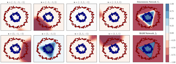
Figure 4: Illustration of the proposed method in Section 3 for a one hidden layer network of size $d_{1}=3$, interpreted as a majority vote over $8$ binary representations ${\mathbf{s}}\in\{-1,1\}^{3}$. For each ${\mathbf{s}}$, a plot shows the values of $F_{{\mathbf{w}}_{2}}({\mathbf{s}})\Psi_{\mathbf{s}}({\mathbf{x}},{\mathbf{W}}_{1})$. The sum of these values gives the deterministic network output $F_{\theta}({\mathbf{x}})$ (see Equation 9). We also show the BAM network output $f_{\theta}({\mathbf{x}})$ for the same parameters $\theta$ (see Equation 6).

Table 4: Selected models overview.

Dataset	Model	Hid. layers	Hid. size	$T$	WD	C	KL	LR	Best epoch
ads	MLP	3	100	-	10-4	-	-	0.1	9
	PBGNetℓ	1	10	100	10-6	11.44	14219	0.1	8
	PBGNet${}_{\ell\text{-bnd}}$	1	10	10	10-6	4.47	2440	0.001	101
	PBGNet	3	10	10000	-	0.47	27	0.01	49
	PBGNet${}_{\text{pre}}$	3	10	10000	-	0.58	0.09	0.1	82
adult	MLP	2	100	-	0	-	-	0.1	21
	PBGNetℓ	1	100	10000	10-6	2.27	13813	0.1	25
	PBGNet${}_{\ell\text{-bnd}}$	1	10	10	0	0.76	1294	0.001	111
	PBGNet	1	10	1000	-	0.30	226	0.1	78
	PBGNet${}_{\text{pre}}$	3	10	10000	-	0.09	0.13	0.01	73
mnist17	MLP	2	50	-	0	-	-	0.01	56
	PBGNetℓ	3	10	100	0	19.99	5068371	0.1	15
	PBGNet${}_{\ell\text{-bnd}}$	1	10	10	10-6	2.82	690	0.001	86
	PBGNet	1	10	10000	-	1.33	164	0.1	106
	PBGNet${}_{\text{pre}}$	1	10	1000	-	0.73	0.46	0.1	71
mnist49	MLP	2	100	-	10-6	-	-	0.001	32
	PBGNetℓ	2	50	10000	0	19.99	819585	0.01	33
	PBGNet${}_{\ell\text{-bnd}}$	1	10	10	0	2.40	1960	0.001	102
	PBGNet	1	10	10000	-	0.90	305	0.1	110
	PBGNet${}_{\text{pre}}$	1	100	10000	-	0.44	1.94	0.1	77
mnist56	MLP	2	50	-	10-6	-	-	0.001	17
	PBGNetℓ	2	10	10000	0	19.99	883939	0.1	26
	PBGNet${}_{\ell\text{-bnd}}$	1	10	10	0	1.95	808	0.001	55
	PBGNet	1	10	10000	-	0.92	192	0.01	95
	PBGNet${}_{\text{pre}}$	1	50	10000	-	0.56	0.70	0.1	84
mnistLH	MLP	3	100	-	10-6	-	-	0.001	55
	PBGNetℓ	3	100	10000	10-6	19.99	98792960	0.1	92
	PBGNet${}_{\ell\text{-bnd}}$	1	10	100	10-6	2.00	8297	0.001	149
	PBGNet	1	10	50	-	0.81	1544	0.1	107
	PBGNet${}_{\text{pre}}$	2	100	10000	-	0.16	0.43	0.01	99

B.3 Additional results

Figure 4 reproduces the experiment presented by Figure 1 with another toy dataset. Table 5 exhibits a variance analysis of Table 1. Figure 6 shows the impact of the training set size. Figure LABEL:fig:sample_effect studies the effect of the sampling size $T$ on the stochastic gradient descent procedure. See figure/table captions for details.

Table 5: Variance analysis of the experiment presented in Table 1. We repeated 20 times the experimental procedure described in Section 6, but with a fixed network architecture of a single hidden layer of 10 neurons to limit computation complexity. Each repetition is executed on different (random) train/test/valid dataset splits, and the stochastic gradient descent is initialized with different random weights. The resulting standard deviations highlight the stability of the models.

Dataset	MLP		PBGNetℓ		PBGNet${}_{\ell\text{-bnd}}$			PBGNet			PBGNet${}_{\text{pre}}$
	ES	ET	ES	ET	ES	ET	Bnd	ES	ET	Bnd	ES	ET	Bnd
ads	0.020	0.034	0.014	0.029	0.026	0.035	0.777	0.112	0.119	0.218	0.046	0.048	0.081
	$\pm$	$\pm$	$\pm$	$\pm$	$\pm$	$\pm$	$\pm$	$\pm$	$\pm$	$\pm$	$\pm$	$\pm$	$\pm$
	0.005	0.007	0.003	0.008	0.003	0.005	0.000	0.003	0.007	0.002	0.007	0.012	0.007
adult	0.133	0.149	0.132	0.148	0.148	0.151	0.271	0.156	0.159	0.215	0.153	0.154	0.166
	$\pm$	$\pm$	$\pm$	$\pm$	$\pm$	$\pm$	$\pm$	$\pm$	$\pm$	$\pm$	$\pm$	$\pm$	$\pm$
	0.007	0.004	0.003	0.003	0.002	0.002	0.002	0.001	0.002	0.001	0.003	0.003	0.002
mnist17	0.002	0.005	0.002	0.005	0.004	0.006	0.102	0.005	0.006	0.041	0.005	0.005	0.010
	$\pm$	$\pm$	$\pm$	$\pm$	$\pm$	$\pm$	$\pm$	$\pm$	$\pm$	$\pm$	$\pm$	$\pm$	$\pm$
	0.001	0.001	0.000	0.001	0.000	0.001	0.004	0.000	0.001	0.001	0.001	0.001	0.001
mnist49	0.003	0.013	0.004	0.016	0.031	0.033	0.300	0.039	0.040	0.143	0.019	0.019	0.031
	$\pm$	$\pm$	$\pm$	$\pm$	$\pm$	$\pm$	$\pm$	$\pm$	$\pm$	$\pm$	$\pm$	$\pm$	$\pm$
	0.002	0.002	0.001	0.003	0.001	0.002	0.000	0.001	0.003	0.001	0.002	0.003	0.002
mnist56	0.004	0.010	0.003	0.010	0.020	0.023	0.186	0.022	0.023	0.090	0.012	0.012	0.020
	$\pm$	$\pm$	$\pm$	$\pm$	$\pm$	$\pm$	$\pm$	$\pm$	$\pm$	$\pm$	$\pm$	$\pm$	$\pm$
	0.001	0.002	0.001	0.002	0.001	0.002	0.000	0.001	0.002	0.001	0.002	0.003	0.002
mnistLH	0.014	0.032	0.017	0.038	0.042	0.049	0.309	0.054	0.056	0.162	0.042	0.042	0.050
	$\pm$	$\pm$	$\pm$	$\pm$	$\pm$	$\pm$	$\pm$	$\pm$	$\pm$	$\pm$	$\pm$	$\pm$	$\pm$
	0.003	0.002	0.001	0.003	0.001	0.003	0.001	0.001	0.002	0.001	0.002	0.002	0.002

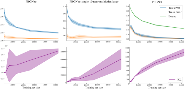
Figure 6: Study of the training sample size effect on PBGNet_ℓ and PBGNet for the biggest dataset, mnistLH. The middle column report results for PBGNet_ℓ with a fixed network architecture of a single hidden layer of 10 neurons, for a direct comparison with PBGNet which always selects this architecture. For each training set size values, 10 repetitions of the learning procedure with different random seeds were performed: each of them executed on different (random) train/test/valid dataset splits, and the stochastic gradient descent is initialized with different random weights. Metrics means of the learned models are displayed by the bold line, with standard deviation shown with the shaded areas. Bound values for PBGNet_ℓ are trivial and thus not reported. We see that PBGNet bound minimization strikingly avoids overfitting by controlling the KL value according to the training set size. On the opposite, PBGNet_ℓ achieves lower test risk, but clearly overfits small training sets.

References

• Ambroladze et al. [2006] Amiran Ambroladze, Emilio Parrado-Hernández, and John Shawe-Taylor. Tighter PAC-Bayes bounds. In NIPS, 2006.
• Bengio [2009] Yoshua Bengio. Learning deep architectures for AI. Foundations and Trends in Machine Learning, 2(1):1–127, 2009.
• Bengio et al. [2013] Yoshua Bengio, Nicholas Léonard, and Aaron C. Courville. Estimating or propagating gradients through stochastic neurons for conditional computation. CoRR, abs/1308.3432, 2013.
• Catoni [2003] Olivier Catoni. A PAC-Bayesian approach to adaptive classification. preprint, 840, 2003.
• Catoni [2004] Olivier Catoni. Statistical learning theory and stochastic optimization: Ecole d’Eté de Probabilités de Saint-Flour XXXI-2001. Springer, 2004.
• Catoni [2007] Olivier Catoni. PAC-Bayesian supervised classification: the thermodynamics of statistical learning, volume 56. Inst. of Mathematical Statistic, 2007.
• Cortes and Vapnik [1995] Corinna Cortes and Vladimir Vapnik. Support-vector networks. Machine Learning, 20(3), 1995.
• Dziugaite and Roy [2017] Gintare Karolina Dziugaite and Daniel M. Roy. Computing nonvacuous generalization bounds for deep (stochastic) neural networks with many more parameters than training data. In UAI. AUAI Press, 2017.
• Germain et al. [2009] Pascal Germain, Alexandre Lacasse, François Laviolette, and Mario Marchand. PAC-Bayesian learning of linear classifiers. In ICML, pages 353–360. ACM, 2009.
• Goodfellow et al. [2016] Ian Goodfellow, Yoshua Bengio, and Aaron Courville. Deep Learning. MIT Press, 2016. http://www.deeplearningbook.org.
• Guedj [2019] Benjamin Guedj. A primer on PAC-Bayesian learning. arXiv preprint arXiv:1901.05353, 2019.
• Hubara et al. [2016] Itay Hubara, Matthieu Courbariaux, Daniel Soudry, Ran El-Yaniv, and Yoshua Bengio. Binarized neural networks. In NIPS, pages 4107–4115, 2016.
• Hubara et al. [2017] Itay Hubara, Matthieu Courbariaux, Daniel Soudry, Ran El-Yaniv, and Yoshua Bengio. Quantized neural networks: Training neural networks with low precision weights and activations. JMLR, 18(1):6869–6898, 2017.
• Kingma and Ba [2015] Diederik P Kingma and Jimmy Ba. Adam: A method for stochastic optimization. In ICLR, 2015.
• Knoblauch et al. [2019] Jeremias Knoblauch, Jack Jewson, and Theodoros Damoulas. Generalized variational inference, 2019.
• Lacasse [2010] Alexandre Lacasse. Bornes PAC-Bayes et algorithmes d’apprentissage. PhD thesis, Université Laval, 2010. URL http://www.theses.ulaval.ca/2010/27635/.
• Langford [2005] John Langford. Tutorial on practical prediction theory for classification. JMLR, 6, 2005.
• Langford and Caruana [2001] John Langford and Rich Caruana. (Not) Bounding the True Error. In NIPS, pages 809–816. MIT Press, 2001.
• Langford and Shawe-Taylor [2002] John Langford and John Shawe-Taylor. PAC-Bayes & margins. In NIPS, 2002.
• Maurer [2004] Andreas Maurer. A note on the PAC-Bayesian theorem. CoRR, cs.LG/0411099, 2004.
• McAllester [1999] David McAllester. Some PAC-Bayesian theorems. Machine Learning, 37(3), 1999.
• McAllester [2003] David McAllester. PAC-Bayesian stochastic model selection. Machine Learning, 51(1), 2003.
• Neyshabur et al. [2018] Behnam Neyshabur, Srinadh Bhojanapalli, and Nathan Srebro. A PAC-Bayesian approach to spectrally-normalized margin bounds for neural networks. In ICLR, 2018.
• Paradis [2018] Frédérik Paradis. Poutyne: A Keras-like framework for PyTorch, 2018. https://poutyne.org.
• Parrado-Hernández et al. [2012] Emilio Parrado-Hernández, Amiran Ambroladze, John Shawe-Taylor, and Shiliang Sun. PAC-Bayes bounds with data dependent priors. JMLR, 13, 2012.
• Paszke et al. [2017] Adam Paszke, Sam Gross, Soumith Chintala, Gregory Chanan, Edward Yang, Zachary DeVito, Zeming Lin, Alban Desmaison, Luca Antiga, and Adam Lerer. Automatic differentiation in PyTorch. In NIPS Autodiff Workshop, 2017.
• Seeger [2002] Matthias Seeger. PAC-Bayesian generalization bounds for gaussian processes. JMLR, 3, 2002.
• Shawe-Taylor and Williamson [1997] John Shawe-Taylor and Robert C. Williamson. A PAC analysis of a Bayesian estimator. In COLT, 1997.
• Soudry et al. [2014] Daniel Soudry, Itay Hubara, and Ron Meir. Expectation backpropagation: Parameter-free training of multilayer neural networks with continuous or discrete weights. In NIPS, pages 963–971, 2014.
• Valiant [1984] Leslie G Valiant. A theory of the learnable. In Proceedings of the sixteenth annual ACM symposium on Theory of computing, pages 436–445. ACM, 1984.
• Williams [1992] Ronald J. Williams. Simple statistical gradient-following algorithms for connectionist reinforcement learning. Machine Learning, 8(3):229–256, May 1992.
• Yin and Zhou [2019] Mingzhang Yin and Mingyuan Zhou. ARM: augment-reinforce-merge gradient for stochastic binary networks. In ICLR (Poster), 2019.
• Yosinski et al. [2014] Jason Yosinski, Jeff Clune, Yoshua Bengio, and Hod Lipson. How transferable are features in deep neural networks? In NIPS, pages 3320–3328, 2014.
• Zhou et al. [2019] Wenda Zhou, Victor Veitch, Morgane Austern, Ryan P. Adams, and Peter Orbanz. Non-vacuous generalization bounds at the imagenet scale: a PAC-bayesian compression approach. In ICLR, 2019.