A Study of Stress-Tensor Distribution around Flux Tube
in Abelian-Higgs Model

Abstract

We study the stress-tensor distribution around the flux tube in static quark and anti-quark systems based on the momentum conservation and the Abelian-Higgs (AH) model. We first investigate constraints on the stress-tensor distribution from the momentum conservation and show that the effect of boundaries plays a crucial role to describe the structure of the flux tube in SU(3) Yang-Mills theory which has measured recently on the lattice. We then study the distributions of the stress tensor and energy density around the magnetic vortex with and without boundaries in the AH model, and compare them with the distributions in SU(3) Yang-Mills theory based on the dual superconductor picture. It is shown that a wide parameter range of the AH model is excluded by a comparison with the lattice results in terms of the stress tensor.

1 Introduction

The energy-momentum tensor (EMT) $\mathcal{T}_{\mu\nu}(x)$ is an important observable in various fields in physics including gravitational theory, hydrodynamics, and elastic body. Among the components of EMT, its spatial part, which is related to the stress tensor $\sigma_{ij}$ as $\sigma_{ij}=-\mathcal{T}_{ij}$ with $i,j=1,2,3$, is a fundamental observable related to force acting on a surface. In field theory, the stress tensor represents distortion of fields induced by external sources Landau . For example, in Maxwell theory local propagation of a Coulomb interaction between charges is characterized by the Maxwell stress, which is the spatial component of the EMT in this theory, $\mathcal{T}_{\mu\nu}=F_{\mu\rho}F^{\rho}_{\;\nu}-(1/4)\delta_{\mu\nu}F_{\rho\sigma}F^{\rho\sigma}$ with the field strength $F_{\mu\nu}$ Landau . The stress tensor in non-Abelian gauge theories including QCD is even more important because this observable characterizes the structure of the non-Abelian fields with external sources in a gauge invariant manner. Recently, the analysis of the stress tensor has been performed in various systems described by the strong interaction, such as the static-quark systems Yanagihara:2018qqg , hadrons Kawamura:2013wfa ; Kumano:2017lhr ; Burkert:2018bqq ; Pagels:1966zza ; Polyakov:2018zvc ; Shanahan:2018pib ; Shanahan:2018nnv , and thermal system having a pressure anisotropy Kitazawa:2019otp .

In Ref. Yanagihara:2018qqg , the stress-tensor distribution in static quark and an anti-quark ($Q\bar{Q}$) systems in SU(3) Yang-Mills (YM) theory has been measured in the numerical simulation of lattice gauge theory. In this study, the analysis of the stress tensor on the lattice is realized with the EMT operator Suzuki:2013gza ; Asakawa:2013laa ; Makino:2014taa ; Kitazawa:2016dsl ; Taniguchi:2016ofw constructed via the gradient flow Narayanan:2006rf ; Luscher:2010iy ; Luscher:2011bx . Through the analysis of the principal directions and eigenvalues of the stress tensor, the formation of the flux tube is revealed in terms of the gauge invariant observable. Before this study, the spatial structure of the flux tube between $Q\bar{Q}$ had been investigated using the color electric field and action density DiGiacomo:1990hc ; Bali:1994de ; Michael:1995pv ; Green:1996be ; Gliozzi:2010zv ; Meyer:2010tw ; Cea:2012qw ; Cardoso:2013lla ; Cea:2015wjd ; Cea:2017ocq (see also the reviews Bali:2000gf ; Greensite ; Kondo:2014sta ). Compared with these previous studies, the use of EMT and especially the stress tensor has several advantages. First, EMT is gauge invariant and an observable having a definite physical meaning related to energy density and force acting on a surface. For example, principal directions of the stress tensor serve as a gauge invariant definition of the direction of “line of force” in non-Abelian theories Yanagihara:2018qqg . Moreover, EMT is a renormalization-group invariant quantity and its absolute value has an unambiguous meaning. Second, as EMT is a second-rank tensor having many channels compared with a vector field, it provides us with more detailed information on the system than the color electric field. In fact, in Ref. Yanagihara:2018qqg it was found that the eigenvalues of EMT on the mid-plane between $Q\bar{Q}$ shows nontrivial degeneracies and separations.

In the present study, motivated by the numerical results in Ref. Yanagihara:2018qqg we explore the distribution of EMT in the $Q\bar{Q}$ system using conservation laws and a specific model. We first discuss constraints on the EMT distribution from the momentum conservation. We show that the transverse structure of the eigenvalues of EMT must have a separation for an infinitely-long flux tube having a translational invariance. This property is qualitatively inconsistent with the lattice results in Ref. Yanagihara:2018qqg . The momentum conservation thus leads to a conclusion that the effect of boundaries of the flux tube is crucial to describe the lattice results.

We then employ the Abelian-Higgs (AH) model and study the EMT distribution around the magnetic vortex with and without boundaries. The AH model is a relativistically generalized version of the Ginzburg-Landau (GL) model for superconductivity. According to the dual superconductor picture Nambu:1974zg ; tHooft:1975krp ; Mandelstam:1974pi ; Nielsen:1973cs , the dual of the AH model is regarded as a phenomenological model of low energy QCD; attempts to derive the dual AH model from QCD have been discussed in the literature Suzuki:1988yq ; Ball:1987cf ; Maedan:1989ju ; Kodama:1997zc based on the Abelian dominance tHooft:1981bkw and the monopole condensation Kronfeld:1987vd ; Kronfeld:1987ri ; Maedan:1988yi . In this picture, magnetic monopoles and the magnetic vortex between the monopoles in the AH model correspond to the color charges and the flux tube in YM theory Nielsen:1973cs , respectively. Based on this picture, the vortex solution in the AH model has been compared with numerical results on the flux tube in YM theory Suganuma:1993ps ; Sasaki:1994sa ; Ichie:1994eg ; Monden:1997hb ; Koma:1999sm ; Koma:2003gq ; Oxman:2017boz ; Oxman:2018dzp . In these studies, however, action density and/or field strength of the color gauge field in a specific gauge have been used for observables to make a comparison.

In the present study, we calculate the spatial distribution of EMT around the magnetic vortex in the AH model, and compare it with the lattice result in Ref. Yanagihara:2018qqg . We demonstrate that the stress-tensor distribution around the infinitely-long magnetic vortex is qualitatively inconsistent with the lattice result, as anticipated from the momentum conservation. We then analyze the magnetic vortex with a finite length, and show that a wide parameter range of the AH model with a standard potential cannot reproduce the lattice result in Ref. Yanagihara:2018qqg simultaneously.

This paper is organized as follows. In Sec. 2, we discuss general properties of the stress-tensor distribution around the flux tube which are obtained only from the momentum conservation and cylindrical symmetry. We then employ the AH model in Sec. 3, and discuss the magnetic vortex in this model with and without boundaries in Sec. 4. In Sec. 5, we discuss the numerical results on the stress-tensor distribution around the magnetic vortex. The final section is devoted to a short summary. Some analytic properties of the vortex solution in the AH model is summarized in Appendix A.

Throughout this paper we consider $3+1$ dimensional Minkowski space with the metric $g^{\mu\nu}={\rm diag}(1,-1,-1,-1)$ with $\mu,\nu=0,1,2,3$.

2 Stress tensor and momentum conservation

In this section, we summarize general properties of the EMT distribution around the flux tube which do not depend on a specific model. In particular, we discuss constraints from the momentum conservation, and show that the lattice results in Ref. Yanagihara:2018qqg are qualitatively inconsistent with the flux tube with an infinite length.

2.1 Stress tensor

The stress tensor is related to the spatial components of EMT as Landau

$$\sigma_{ij}=-\mathcal{T}_{ij}\quad(i,j=1,2,3).$$ (2.1)

Force per unit area ${\cal F}_{i}$ acting on a surface with the normal vector $n_{i}$ is represented in terms of the stress tensor as

$${\cal F}_{i}=\sigma_{ij}n_{j}=-{\cal T}_{ij}n_{j}.$$ (2.2)

From Eq. (2.2) one sees that the force and the normal vector are parallel only for the local principal axes obtained by solving the eigenvalue equations

$${\cal T}_{ij}n_{j}^{(k)}=\lambda_{k}n_{i}^{(k)}\quad(k=1,2,3).$$ (2.3)

The strength of the force per unit area along $n_{i}^{(k)}$ is given by the eigenvalue $\lambda_{k}$. Neighboring volume elements separated by a surface with the normal vector $n_{i}^{(k)}$ are pulling (pushing) with each other for $\lambda_{k}<0$ ($\lambda_{k}>0$) on the surface. As $\sigma_{ij}$ is a symmetric tensor, three principal axes $n_{i}^{(k)}$ are orthogonal with each other.

Let us see two examples of EMT and stress tensor. First, in a thermal medium with an infinite volume EMT is given by

$${\cal T}_{\mu\nu}={\rm diag}(\varepsilon,P,P,P),$$ (2.4)

with energy density $\varepsilon$ and pressure $P>0$. As the stress tensor reads $\sigma_{ij}=-P\delta_{ij}$, force acting on a surface element is always perpendicular to the surface. The sign of the eigenvalues means that volume elements are pushing with each other with pressure $P$. Second, in Maxwell theory for electromagnetism EMT is given by

$$\mathcal{T}_{\mu\nu}=F_{\mu\rho}F^{\rho}_{\nu}-\frac{1}{4}\delta_{\mu\nu}F_{\rho\sigma}F^{\rho\sigma},$$ (2.5)

with the field strength $F_{\mu\nu}$. When a static electric or magnetic field along the $z$ direction is applied as $\vec{E}=(0,0,E)$ or $\vec{B}=(0,0,B)$, one has

$${\cal T}_{\mu\nu}=\frac{1}{2}{\rm diag}(E^{2},E^{2},E^{2},-E^{2}),\quad\mbox{or}\quad{\cal T}_{\mu\nu}=\frac{1}{2}{\rm diag}(B^{2},B^{2},B^{2},-B^{2}),$$ (2.6)

respectively. Equation (2.6) shows that volume elements are pulling with each other along the direction of $\vec{E}$, while volume elements are pushing with each other along directions perpendicular to $\vec{E}$ Landau . In Eq. (2.6), all absolute values of the eigenvalues of ${\cal T}_{\mu\nu}$ are identical, and the principal axis associated with the negative eigenvalue $\lambda_{i}$ is parallel to the field $\vec{E}$ or $\vec{B}$. This principal axis thus corresponds to the direction of the line of force in Maxwell theory.

In a static system, the momentum conservation implies

$$\partial_{i}\mathcal{T}^{ij}=0.$$ (2.7)

By taking a volume integral of Eq. (2.7) on a volume $V$ without external charges and using the Gauss theorem, one obtains

$$\int_{V}dV\,\partial_{i}\mathcal{T}^{ij}=\int_{S}dS_{i}\,\mathcal{T}^{ij}=0,$$ (2.8)

where $S$ is the surface of $V$ with the outgoing surface vector. Since $dS_{i}\mathcal{T}^{ij}$ is the $j$-th component of force acting on the surface element $dS_{i}$, Eq. (2.8) represents the equilibrium of force acting on $V$ through its surface. When there exists a test charge in volume $V$, force $\vec{F}$ acting on the test charge is related to the surface integral as ${F}_{i}=-\int_{S}{\cal T}_{ij}dS_{j}$.

2.2 Cylindrical coordinate system

In the analysis of the flux tube or magnetic vortex, it is convenient to employ the cylindrical coordinate system $(r,\theta,z)$ with $r=\sqrt{x^{2}+y^{2}}$ and $\theta=\tan^{-1}(y/x)$ with $0\leq\theta<2\pi$ because of the rotational symmetry around an axis. The components of EMT in this coordinate system are given by

$$\mathcal{T}_{\gamma\gamma^{\prime}}(r,z)=(e_{\gamma})_{\mu}\mathcal{T}^{\mu\nu}(e_{\gamma^{\prime}})_{\nu},$$ (2.9)

with $\gamma,\gamma^{\prime}=0,r,\theta,z$ and $e_{\gamma}$ denotes a unit vector along the direction of the $\gamma$ axis in the Minkowski space.

The momentum conservation Eq. (2.7) in terms of $\mathcal{T}_{\gamma\gamma^{\prime}}(r,z)$ is given by

$$\frac{1}{r}\partial_{r}(r\mathcal{T}_{rr})-\frac{\mathcal{T}_{\theta\theta}}{r}+\partial_{z}\mathcal{T}_{rz}=0,$$ (2.10)

$$\partial_{\theta}\mathcal{T}_{\theta\theta}=0,$$ (2.11)

$$\frac{1}{r}\partial_{r}(r\mathcal{T}_{rz})+\partial_{z}\mathcal{T}_{zz}=0,$$ (2.12)

which represents the equilibrium of force acting on an infinitesimal volume element along the $r,\theta,z$ directions, respectively.

When a system is translationally symmetric along $z$ direction in addition to the rotational symmetry, the components of EMT is given by functions of $r$ as ${\cal T}_{\gamma\gamma^{\prime}}={\cal T}_{\gamma\gamma^{\prime}}(r)$, and $z$ derivatives in Eqs. (2.10)–(2.12) vanish. Only a non-trivial constraint from the momentum conservation is then obtained from Eq. (2.10) as

$$\partial_{r}(r\mathcal{T}_{rr}(r))=\mathcal{T}_{\theta\theta}(r).$$ (2.13)

By rewriting Eq. (2.13) as $r\partial_{r}(\mathcal{T}_{rr}(r))=\mathcal{T}_{\theta\theta}(r)-\mathcal{T}_{rr}(r)$ it is easy to show that $\mathcal{T}_{rr}(r)$ and $\mathcal{T}_{\theta\theta}(r)$ behave differently as functions of $r$ except for the case $\mathcal{T}_{rr}(r)=\mathcal{T}_{\theta\theta}(r)=0$ provided that $\mathcal{T}_{rr}(r)\to 0$ in the $r\to\infty$ limit. Moreover, by integrating out both sides of Eq. (2.13) and assuming $r\mathcal{T}_{rr}(r)|_{r\to\infty}=r\mathcal{T}_{rr}(r)|_{r\to 0}=0$ one obtains

$$\int_{0}^{\infty}dr\,{\cal T}_{\theta\theta}(r)=0,$$ (2.14)

which shows that ${\cal T}_{\theta\theta}(r)$ as a function of $r$ must change sign at least once so that its integral vanishes.

2.3 Lattice results on flux tube in SU(3) YM theory

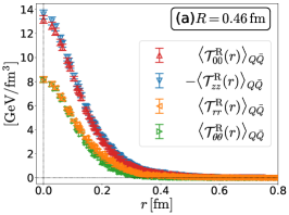
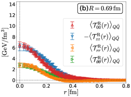
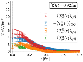
Figure 1: Distribution of EMT on the mid-plane of the flux tube obtained from the lattice numerical simulation in SU(3) YM theory Yanagihara:2018qqg . The lengths of the flux tube are $R=0.46,$ $0.69,$ and $0.92$ fm for (a), (b), and (c), respectively.

Now let us inspect the components of EMT on the mid-plane of the flux tube in SU(3) YM theory obtained on the lattice in Ref. Yanagihara:2018qqg . In Fig. 1 we show the expectation values of ${\cal T}_{00}(r)$, ${\cal T}_{zz}(r)$, ${\cal T}_{rr}(r)$, and ${\cal T}_{\theta\theta}(r)$ on the mid-plane in the $Q\bar{Q}$ system as functions of $r$ for three $Q\bar{Q}$ distances, $R=0.46$, $0.69$, and $0.92$ fm. The figure shows that ${\cal T}_{rr}(r)$ and ${\cal T}_{\theta\theta}(r)$ are degenerated within statistics for all $Q\bar{Q}$ distances. Moreover, the result suggests $\int_{0}^{\infty}dr{\cal T}_{\theta\theta}(r)>0$. These properties do not agree with Eqs. (2.13) and (2.14) obtained by assuming the translational invariance. Therefore, the result in Fig. 1 shows that the assumption of translational invariance is not applicable to the flux tube in SU(3) YM theory even on the mid-plane with $R=0.92$ fm.

3 Abelian-Higgs model

3.1 Model

Now we employ the Abelian-Higgs (AH) model and investigate the EMT distribution around the magnetic vortex with and without boundaries. Our starting point is the AH Lagrangian in four-dimensional Minkowski space:

$$\mathcal{L}_{\mathrm{AH}} =-\frac{1}{4g^{2}}(\partial_{\mu}A_{\nu}(x)-\partial_{\nu}A_{\mu}(x))^{2}+|(\partial_{\mu}+iA_{\mu}(x))\chi(x)|^{2}-\lambda(|\chi(x)|^{2}-v^{2})^{2}$$

$$=-\frac{1}{4g^{2}}F_{\mu\nu}^{2}(x)+|D_{\mu}\chi(x)|^{2}-V(|\chi(x)|),$$ (3.1)

where $F_{\mu\nu}(x)=\partial_{\mu}A_{\nu}(x)-\partial_{\nu}A_{\mu}(x)$ and $D_{\mu}=\partial_{\mu}+iA_{\mu}(x)$ are the field strength tensor and the covariant derivative, respectively, with the Abelian gauge field $A_{\mu}(x)$ and the complex scalar field $\chi(x)$. The last term $V(|\chi(x)|)=\lambda(|\chi(x)|^{2}-v^{2})^{2}$ represents the Higgs potential which induces the scalar condensation. The AH model has three parameters, $g$, $\lambda$, and $v$. $g$ is the gauge coupling constant, and $v$ is the vacuum expectation value of $\chi(x)$. The EMT in the AH model is obtained as a Noether current of the translational symmetry as Bogomolnyi:1976 ; deVega:1976xbp

$$\mathcal{T}_{\mu\nu}(x)=(D_{\mu}\chi(x))^{*}(D_{\nu}\chi(x))+(D_{\nu}\chi(x))^{*}(D_{\mu}\chi(x))-\frac{1}{g^{2}}g^{\rho\sigma}F_{\mu\rho}(x)F_{\nu\sigma}(x)-g_{\mu\nu}\mathcal{L}.$$ (3.2)

The AH model has two characteristic length scales; the correlation lengths of the scalar and gauge fields Fetter ,

$$\xi_{\chi}=\frac{1}{2\sqrt{\lambda}v},\quad\xi_{A}=\frac{1}{\sqrt{2}gv},$$ (3.3)

respectively. The ratio of these two scales characterizes the Ginzburg-Landau (GL) parameter $\kappa$,

$$\kappa=\frac{\xi_{\chi}}{\sqrt{2}\xi_{A}}=\frac{\sqrt{\lambda}}{g}.$$ (3.4)

In the context of superconductivity, the GL parameter classifies the type of superconductor into type-I ($\kappa<1/\sqrt{2}$) or type-II ($\kappa>1/\sqrt{2}$). In the type-I superconductor, the interaction between vortices is attractive so that a system of two and more individual vortices is unstable for the formation of a single vortex with a multiple winding number. In contrast, the interaction between vortices is repulsive in the type-II superconductor Fetter . The boundary value $\kappa=1/\sqrt{2}$ is called the Bogomol’nyi bound Bogomolnyi:1976 .

The AH Lagrangian is invariant under the U(1) gauge transformation defined by

$$\chi(x)\rightarrow\chi(x)e^{i\alpha(x)},\quad\chi^{*}(x)\rightarrow\chi^{*}(x)e^{-i\alpha(x)},\quad A_{\mu}(x)\rightarrow A_{\mu}(x)-\partial_{\mu}\alpha(x),$$ (3.5)

with a gauge function $\alpha(x)$. The complex scalar field $\chi(x)$ is written as

$$\chi(x)=\phi(x)e^{if(x)},$$ (3.6)

with a real scalar field $\phi(x)$ and a phase function $f(x)$. In the unitary gauge defined by $\alpha(x)=-f(x)$, we have the gauge-fixed AH Lagrangian,

$$\mathcal{L}_{\mathrm{AH}}=-\frac{1}{4g^{2}}(\partial_{\mu}A^{\prime}_{\nu}(x)-\partial_{\nu}A^{\prime}_{\mu}(x))^{2}+|(\partial_{\mu}+iA^{\prime}_{\mu}(x))\phi(x)|^{2}-\lambda(\phi(x)^{2}-v^{2})^{2},$$ (3.7)

with $A^{\prime}_{\mu}(x)=A_{\mu}(x)+\partial_{\mu}f(x)$.

3.2 Energy-momentum tensor in cylindrical coordinate system

In this study we investigate the spatial distribution of EMT around the magnetic vortex with and without boundaries. As these systems possess rotational symmetry around the vortex, we employ the cylindrical coordinate system. For the vortex with length $R$, we suppose that the boundaries are at $(r,z)=(0,\pm R/2)$. From the rotational symmetry the scalar field is given by a functions of $r$ and $z$ as

$$\phi=\phi(r,z),$$ (3.8)

and it is possible to represent the gauge field as

$$\vec{A}(r,z)=\frac{\tilde{A}(r,z)}{r}\vec{e}_{\theta}.$$ (3.9)

with a scalar function $\tilde{A}(r,z)$ and the three-dimensional unit vector $\vec{e}_{\theta}$ in the direction of the $\theta$ axis.

The non-vanishing components of EMT in the cylindrical coordinate system, Eq. (2.9), are calculated to be

$$\mathcal{T}_{00}(r,z)=\frac{1}{2g^{2}r^{2}}\Bigl{(}(\partial_{r}\tilde{A})^{2}+(\partial_{z}\tilde{A})^{2}\Bigr{)}+\Bigl{(}(\partial_{r}\phi)^{2}+(\partial_{z}\phi)^{2}\Bigr{)}+\frac{\phi^{2}\tilde{A}^{2}}{r^{2}}+\lambda(\phi^{2}-v^{2})^{2},$$ (3.10)

$$\mathcal{T}_{rr}(r,z)=\frac{1}{2g^{2}r^{2}}\Bigl{(}(\partial_{r}\tilde{A})^{2}-(\partial_{z}\tilde{A})^{2}\Bigr{)}+\Bigl{(}(\partial_{r}\phi)^{2}-(\partial_{z}\phi)^{2}\Bigr{)}-\frac{\phi^{2}\tilde{A}^{2}}{r^{2}}-\lambda(\phi^{2}-v^{2})^{2},$$ (3.11)

$$\mathcal{T}_{\theta\theta}(r,z)=\frac{1}{2g^{2}r^{2}}\Bigl{(}(\partial_{r}\tilde{A})^{2}+(\partial_{z}\tilde{A})^{2}\Bigr{)}-\Bigl{(}(\partial_{r}\phi)^{2}+(\partial_{z}\phi)^{2}\Bigr{)}+\frac{\phi^{2}\tilde{A}^{2}}{r^{2}}-\lambda(\phi^{2}-v^{2})^{2},$$ (3.12)

$$\mathcal{T}_{zz}(r,z)=\frac{-1}{2g^{2}r^{2}}\Bigl{(}(\partial_{r}\tilde{A})^{2}-(\partial_{z}\tilde{A})^{2}\Bigr{)}-\Bigl{(}(\partial_{r}\phi)^{2}-(\partial_{z}\phi)^{2}\Bigr{)}-\frac{\phi^{2}\tilde{A}^{2}}{r^{2}}-\lambda(\phi^{2}-v^{2})^{2},$$ (3.13)

$$\mathcal{T}_{rz}(r,z)=\frac{1}{g^{2}r^{2}}(\partial_{r}\tilde{A})(\partial_{z}\tilde{A})+2(\partial_{r}\phi)(\partial_{z}\phi).$$ (3.14)

On the mid-plane at $z=0$, $\mathcal{T}_{rz}(r,z=0)$ vanishes from the symmetric reason and EMT is diagonalized as

$$\mathcal{T}_{\gamma\gamma^{\prime}}(r)=\mathrm{diag}(\mathcal{T}_{00}(r),\mathcal{T}_{rr}(r),\mathcal{T}_{\theta\theta}(r),\mathcal{T}_{zz}(r)),$$ (3.15)

where the argument $z=0$ in $\mathcal{T}_{\gamma\gamma^{\prime}}(r,z)$ is abbreviated for notational simplicity. Each component is given by

$$\mathcal{T}_{00}(r)=-\mathcal{T}_{zz}(r)= \frac{1}{2g^{2}r^{2}}(\partial_{r}\tilde{A})^{2}+(\partial_{r}\phi)^{2}+\frac{\phi^{2}\tilde{A}^{2}}{r^{2}}+\lambda(\phi^{2}-v^{2})^{2},$$ (3.16)

$$\mathcal{T}_{rr}(r)= \frac{1}{2g^{2}r^{2}}(\partial_{r}\tilde{A})^{2}+(\partial_{r}\phi)^{2}-\frac{\phi^{2}\tilde{A}^{2}}{r^{2}}-\lambda(\phi^{2}-v^{2})^{2},$$ (3.17)

$$\mathcal{T}_{\theta\theta}(r)= \frac{1}{2g^{2}r^{2}}(\partial_{r}\tilde{A})^{2}-(\partial_{r}\phi)^{2}+\frac{\phi^{2}\tilde{A}^{2}}{r^{2}}-\lambda(\phi^{2}-v^{2})^{2},$$ (3.18)

where we used the fact that terms including $\partial_{z}$ vanish on the mid-plane.

Equations (3.16)–(3.18) tell us several notable features. First, the absolute values of $\mathcal{T}_{00}(r)$ and $\mathcal{T}_{zz}(r)$ on the mid-plane always degenerate in the AH model. Second, the first term of Eqs. (3.16)–(3.18) corresponds to the Maxwell stress Eq. (2.5). On the mid-plane, direction of the magnetic field is along the $z$ axis. As a result, as in Eq. (2.6) this term gives a negative (positive) contribution to $\mathcal{T}_{zz}(r)$ ($\mathcal{T}_{rr}(r)$ and $\mathcal{T}_{\theta\theta}(r)$). Third, the last term is a contribution from the Higgs potential. The contribution of this term is negative for all spatial components $\mathcal{T}_{zz}(r)$, $\mathcal{T}_{rr}(r)$, and $\mathcal{T}_{\theta\theta}(r)$, while the contribution to $\mathcal{T}_{00}(r)$ is positive. These contributions are understood as the negative pressure owing to the instability of a state having a deviation of $\phi$ from its vacuum expectation value $v$. Fourth, because $\mathcal{T}_{rr}(r)=\mathcal{T}_{\theta\theta}(r)$ at $r=0$, one obtains $(\partial_{r}\phi)^{2}=\phi^{2}\tilde{A}^{2}/r^{2}$ in the $r\to 0$ limit. As a result, the signs of $\mathcal{T}_{rr}(r)$ and $\mathcal{T}_{\theta\theta}(r)$ at $r=0$ is determined by the interplay between first and fourth terms, i.e. contributions from the gauge field and the Higgs potential, respectively.

4 Magnetic vortex

In this section, we discuss the magnetic monopoles and the classical solution of the magnetic vortex between the monopoles in the AH model with and without boundaries.

4.1 Magnetic vortex with finite length

Let us first consider a magnetic vortex with the finite length $R$ between two magnetic monopoles with opposite charges. As shown by Dirac Dirac:1931kp , Maxwell theory can have monopoles with quantized charges. These monopoles are associated with a singularity of the gauge field called the Dirac string. When two monopoles with opposite charges are at $(r,z)=(0,\pm R/2)$, the Dirac string can be located on the $z$ axis between two monopoles. The gauge field in this case is given by

$$\vec{A}^{D}(r,z)=-\frac{n}{2r}\biggl{(}\frac{z+R/2}{\sqrt{r^{2}+(z+R/2)^{2}}}-\frac{z-R/2}{\sqrt{r^{2}+(z-R/2)^{2}}}\biggr{)}\vec{e}_{\theta}=\frac{\tilde{A}^{D}(r,z)}{r}\vec{e}_{\theta},$$ (4.1)

where the winding number $n$ corresponds to the charge of a monopole at $z=R/2$ in the unit of $2\pi/g$. One easily finds that the magnetic field $\vec{B}^{D}=\nabla\times\vec{A}^{D}$ is given by the superposition of the Coulombic fields with the charges $\pm 2n\pi/g$ at $(r,z)=(0,\pm R/2)$. The magnetic field at the origin thus is given by

$$|\vec{B}(0)|=2\frac{2n\pi}{g}\frac{1}{4\pi(R/2)^{2}}=\frac{4n}{gR^{2}}.$$ (4.2)

Substituting Eq. (4.2) into Eq. (2.6), one obtains

$$\mathcal{T}_{00}(0)=\mathcal{T}_{rr}(0)=\mathcal{T}_{\theta\theta}(0)=\frac{8n^{2}}{g^{2}R^{4}},\quad\mathcal{T}_{zz}(0)=-\frac{8n^{2}}{g^{2}R^{4}},$$ (4.3)

on the mid-plane. In what follows, we consider the vortex with $n=1$.

The Dirac monopoles can also be introduced in the AH model. As the gauge field in this case has the same singularity as Eq. (4.1), when monopoles are located at $(r,z)=(0,\pm R/2)$ it is convenient to denote the gauge field as Koma:2003gq ; Maedan:1989ju ; Kodama:1997zc

$$\vec{A}(r,z)=\vec{A}^{D}(r,z)+\vec{a}(r,z),$$ (4.4)

$$\vec{a}=a(r,z)\vec{e}_{\theta}=\frac{\tilde{a}(r,z)}{r}\vec{e}_{\theta}.$$ (4.5)

Here, $\tilde{a}(r,z)$ does not have a singularity and represents the deviation of $\vec{A}(r,z)$ from Eq. (4.1). The classical solution of the magnetic vortex is then obtained by minimizing the total energy

$$E=\int d^{3}x\,\mathcal{T}_{00}(r,z)=2\pi\int_{0}^{\infty}rdr\int_{-\infty}^{\infty}dz\,\mathcal{T}_{00}(r,z),$$ (4.6)

as a functional of $\tilde{a}(r,z)$ and $\phi(r,z)$ with the boundary conditions

$$\tilde{a}(r,z)\rightarrow 0 \mathrm{for}\,\,r\rightarrow 0,\,\,\forall z$$ (4.7)

$$\phi(r,z)\rightarrow 0\quad \mathrm{for}\,\,r\rightarrow 0,\,\,-R/2\leq z\leq R/2,$$ (4.8)

$$\tilde{a}(r,z)\rightarrow-\tilde{A}^{D}(r,z),\,\phi(r,z)\rightarrow v \mathrm{for}\,\,r,\,z\rightarrow\infty.$$ (4.9)

The condition Eq. (4.9) ensures that the total energy of this system is finite.

We note that $\tilde{a}(r,z)$ and $\phi(r,z)$ hardly change within the length $\xi_{A}$ and $\xi_{\chi}$. Therefore, when the condition $R\ll\xi_{A},\xi_{\chi}$ is satisfied, they remain Eqs. (4.7) and (4.8) and take values almost equal to zero around the monopoles. In this case, the EMT around the monopoles should be dominated by the contribution from the gauge field $\vec{A}^{D}(r,z)$.

4.2 Infinitely-long vortex

Next we consider the magnetic vortex with an infinite length. This solution is obtained by taking the $R\to\infty$ limit in the above argument. In this limit, the system has a translational symmetry along $z$ direction, and $\phi$ and $\tilde{a}$ are given by functions of only $r$ as $\phi=\phi(r)$ and $\tilde{a}=\tilde{a}(r)$. By taking the $R\to\infty$ limit of Eq. (4.1) with $n=1$ one obtains

$$\tilde{A}^{D}(r,z)=-1.$$ (4.10)

The vortex solution is obtained by minimizing energy per unit length

$$\int_{0}^{\infty}(2\pi r)dr{\cal T}_{00}(r)$$ (4.11)

with respect to $\phi(r)$ and $\tilde{a}(r)$ with the boundary conditions

$$\tilde{a}(r)\rightarrow 0,\,\phi(r)\rightarrow 0 \quad\mathrm{for~{}}r\rightarrow 0,$$ (4.12)

$$\tilde{a}(r)\rightarrow 1,\,\phi(r)\rightarrow v \quad\mathrm{for~{}}r\rightarrow\infty.$$ (4.13)

It is convenient to introduce dimensionless variables

$$\rho=rgv,\quad P(\rho)=\frac{\phi(\rho/gv)}{v},\quad Q(\rho)=\tilde{A}(\rho/gv).$$ (4.14)

Using these variables, the components of the dimensionless EMT

$$\hat{\mathcal{T}}_{\gamma\gamma^{\prime}}(\rho)=\frac{\xi_{A}^{2}}{v^{2}}\mathcal{T}_{\gamma\gamma^{\prime}}\Big{(}\frac{\rho}{gv}\Big{)}$$ (4.15)

are given by

$$\hat{\mathcal{T}}_{00}(\rho)=-\hat{\mathcal{T}}_{zz}(\rho) =\hat{T}_{(1)}(\rho)+\hat{T}_{(2)}(\rho)+\hat{T}_{(3)}(\rho)+\hat{T}_{(4)}(\rho),$$ (4.16)

$$\hat{\mathcal{T}}_{rr}(\rho) =\hat{T}_{(1)}(\rho)+\hat{T}_{(2)}(\rho)-\hat{T}_{(3)}(\rho)-\hat{T}_{(4)}(\rho),$$ (4.17)

$$\hat{\mathcal{T}}_{\theta\theta}(\rho) =\hat{T}_{(1)}(\rho)-\hat{T}_{(2)}(\rho)+\hat{T}_{(3)}(\rho)-\hat{T}_{(4)}(\rho),$$ (4.18)

with

$$\hat{T}_{(1)}(\rho)=\frac{(\partial_{\rho}Q)^{2}}{4\rho^{2}},\quad\hat{T}_{(2)}(\rho)=\frac{(\partial_{\rho}P)^{2}}{2},\quad\hat{T}_{(3)}(\rho)=\frac{P^{2}Q^{2}}{2\rho^{2}},\quad\hat{T}_{(4)}(\rho)=\frac{\kappa^{2}(P^{2}-1)^{2}}{2}.$$ (4.19)

Energy per unit length Eq. (4.11) is represented as

$$\int_{0}^{\infty}(2\pi r)dr{\cal T}_{00}(r)=2\pi v^{2}\hat{\Sigma}[P,Q],$$ (4.20)

with

$$\hat{\Sigma}[P,Q]=2\int_{0}^{\infty}\rho d\rho\hat{\cal T}_{00}(\rho)=\int_{0}^{\infty}\rho d\rho\biggl{[}\frac{1}{2\rho^{2}}(\partial_{\rho}Q)^{2}+(\partial_{\rho}P)^{2}+\frac{P^{2}Q^{2}}{\rho^{2}}+\kappa^{2}(P^{2}-1)^{2}\biggr{]}.$$ (4.21)

In Eq. (4.21), the form of $\hat{\Sigma}[P,Q]$ depends on parameters in the AH model only through $\kappa$. Therefore, $P(\rho)$ and $Q(\rho)$ of the vortex solution, and accordingly the dimensionless EMT Eq. (4.15), depend only on $\kappa$. Also, the energy per unit length, i.e. the string tension of the vortex, $\sigma_{\rm AH}$, is given by

$$\sigma_{\rm AH}=2\pi v^{2}\hat{\sigma}_{\rm AH}(\kappa),$$ (4.22)

where $\hat{\sigma}_{\rm AH}(\kappa)$ is obtained by substituting the vortex solution into $\hat{\Sigma}[P,Q]$. As shown in Appendix A, it is possible to show $\hat{\sigma}_{\rm AH}(1/\sqrt{2})=1$ analytically Bogomolnyi:1976 .

4.3 Physical units

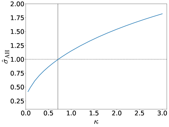
Figure 2: Behavior of $\hat{\sigma}_{\rm AH}(\kappa)$. The vertical line shows the Bogomol’nyi bound $\kappa=1/\sqrt{2}$.

To compare the stress-tensor distribution around the magnetic vortex obtained in the AH model with the flux tube in Ref. Yanagihara:2018qqg , it is desirable to introduce the physical dimension to the former. The only parameter having a mass dimension in the AH model is $v$. To determine this quantity in physical units, we require that the string tension of the magnetic vortex $\sigma_{\rm AH}$ is equivalent with the string tension of the flux tube in SU(3) YM theory, $\sigma_{\rm YM}$ Suganuma:1993ps ; Kodama:1997zc . From Eq. (4.22), we then have

$$v=\sqrt{\frac{\sigma_{\rm YM}}{2\pi\hat{\sigma}_{\rm AH}(\kappa)}}.$$ (4.23)

The value of $\hat{\sigma}_{\rm AH}(\kappa)$ is obtained numerically from the solution of the magnetic vortex with an infinite length. In Fig. 2, we show the behavior of $\hat{\sigma}_{\rm AH}(\kappa)$ as a function of $\kappa$. The figure shows that $\hat{\sigma}_{\rm AH}=1$ at $\kappa=1/\sqrt{2}$. This property can be shown analytically Bogomolnyi:1976 , as discussed in Appendix A.

For the value of $\sigma_{\rm YM}$, we use

$$\sigma_{\rm YM}=1.132(10)~{}{\rm GeV/fm},$$ (4.24)

which is obtained from the large $R$ behavior of the $Q\bar{Q}$ potential at $\beta=6.6$ in Ref. Yanagihara:2018qqg .

Because the right-hand side of Eq. (4.23) depends only on $\kappa$, even after fixing the value of $v$ in physical units, there exists an arbitrariness to vary $g$ and $\lambda$ with fixed $\kappa=\sqrt{\lambda}/g$. This means that $\xi_{\chi}$ and $\xi_{A}$ are not determined by fixing $v$ and $\kappa$. This arbitrariness is canceled out in Eq. (4.15) for the infinitely-long case, but has to be taken into account explicitly when $R$ is finite.

4.4 Details of numerical analysis

The classical solution of the magnetic vortex is obtained numerically by minimizing the total energy with the boundary conditions Eq. (4.12) and (4.13). For this procedure with finite length $R$ we discretize the half-plane of $r$ and $z$ and iteratively update the fields $\phi(r,z)$ and $\tilde{a}(r,z)$ at even and odd sites via the over-relaxation method. We take the mesh size $\Delta$ of the lattice as

$$\Delta=p~{}{\rm min}(\xi_{A},\xi_{\chi})$$ (4.25)

where $p$ is chosen in the range $0.02<p<0.1$ so that the ratio of $R$ and $2\Delta$ is given by an integer. We have checked that the mesh size with $p=0.1$ is small enough to suppress the discretization error in the range $0.1<\kappa<1.0$ by changing the mesh size. The spatial lengths along $r$ and $z$ directions are chosen so that the boundaries are at least $3.4$ times longer than ${\rm max}(\xi_{A},\xi_{\chi})$. We have checked that the finite size effects are well suppressed with this setting. The iteration is terminated when the total energy becomes unchanged in each step. The criterion is set to be $\delta E=(E_{n+1}-E_{n})/E_{n}<1.0\times 10^{-6}$ for the $n$-th iteration. Once we obtain the solution for $\phi$ and $\tilde{a}$, EMT is obtained by substituting them into Eqs. (3.10)–(3.13).

For the infinitely-long case we proceed similar procedures in the one dimensional space of $\rho$ for the dimensionless functions $P(\rho)$ and $Q(\rho)$.

We note that the number of lattice points increases when the difference between $\xi_{A}$ and $\xi_{\chi}$ is large in order to satisfy the above conditions for the mesh size $\Delta$ and the size of the lattice. This means that the numerical cost increases at small and large $\kappa$. Because of this difficulty, we limit our numerical analysis in the range $0.1\leq\kappa\leq 1.0$ and $0.05\leq\kappa\leq 3.0$ for the finite-length and infinitely-long vortices, respectively.

5 Numerical results

In this section we discuss the numerical results on the EMT distribution around the magnetic vortex in the AH model.

5.1 Infinitely-long vortex

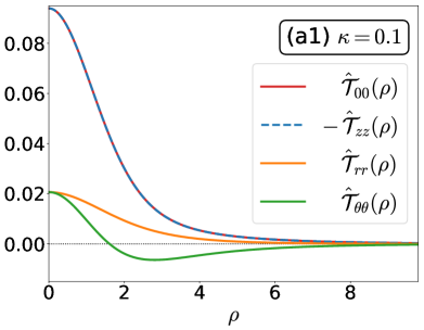
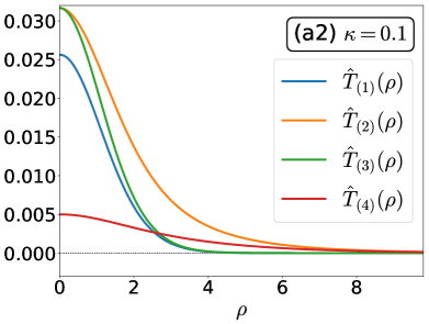
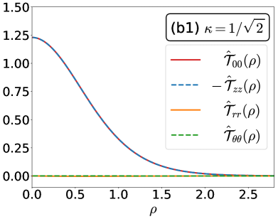
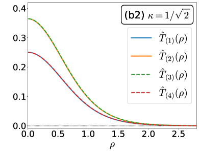
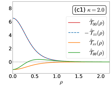
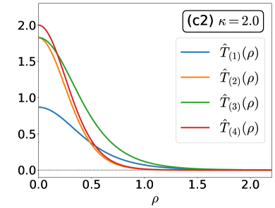
Figure 3: EMT distribution around the infinitely-long flux tube (left) and the contributions of individual terms in Eq. (4.19) (right). Top, middle, and bottom panels show the results for $\kappa=0.1$, $\kappa=1/\sqrt{2}$, and $\kappa=2.0$, respectively.

In this subsection, we first focus on the infinitely-long vortex. In this case it is convenient to employ the dimensionless variables, $\rho$ and $\hat{\mathcal{T}}_{\gamma\gamma}(\rho)$, introduced in Eqs. (4.14) and (4.15), which depend only on $\kappa$. In the left panels of Fig. 3, we show the $\rho$ dependences of $\hat{\mathcal{T}}_{00}(\rho)$, $\hat{\mathcal{T}}_{zz}(\rho)$, $\hat{\mathcal{T}}_{rr}(\rho)$, and $\hat{\mathcal{T}}_{\theta\theta}(\rho)$ for three values of $\kappa$; top and lower panels show the results for type-I ($\kappa=0.1$) and type-II ($\kappa=2.0$) cases, respectively, while the middle panel corresponds to the Bogomol’nyi bound at $\kappa=1/\sqrt{2}$. One finds that the sign of $\mathcal{T}_{rr}(r)$ is positive (negative) at $\kappa=0.1$ ($\kappa=2.0$), while the middle panel shows that $\mathcal{T}_{rr}(r)=\mathcal{T}_{\theta\theta}(r)=0$ at $\kappa=1/\sqrt{2}$. The latter property is obtained analytically as discussed in Refs. Bogomolnyi:1976 ; deVega:1976xbp and summarized in Appendix A. For $\kappa\neq 1/\sqrt{2}$, $\mathcal{T}_{\theta\theta}(r)$ behaves differently from $\mathcal{T}_{rr}(r)$, and changes the sign at nonzero $r$. This result is consistent with the discussion based on the momentum conservation in Sec. 2.

Now, let us compare the result in Fig. 3 with the EMT distribution around the flux tube in SU(3) YM theory Yanagihara:2018qqg shown in Fig. 1. As in Fig. 1, in SU(3) YM theory $\mathcal{T}_{rr}(r)$ and $\mathcal{T}_{\theta\theta}(r)$ are degenerated within statistics even at the largest $Q\bar{Q}$ distance, $R=0.92$ fm. The lattice result also suggests that $\mathcal{T}_{\theta\theta}(r)$ is always positive. These results clearly contradict with Fig. 3. This result thus shows that the structure of the flux tube in SU(3) YM theory with $R\leq 0.92$ fm cannot be understood by the comparison with the magnetic vortex with an infinite length in the AH model.

Figure 4: $\kappa$-dependence of the ratio $\mathcal{T}_{rr}(0)/\mathcal{T}_{00}(0)$ for the infinitely-long vortex. The value $\kappa=1/\sqrt{2}$ is indicated by the vertical line.

In spite of this conclusion, it is instructive to take a closer look at the EMT distribution in the AH model in Fig. 3. As in Eqs. (4.16)–(4.18), the EMT around the infinitely-long vortex consists of four terms in Eq. (4.19). In the right panels of Fig. 3, the behavior of these terms are shown separately for each $\kappa$. At $\rho=0$, one has $\hat{T}_{(2)}(\rho)=\hat{T}_{(3)}(\rho)$ which leads to $\mathcal{T}_{rr}(0)=\mathcal{T}_{\theta\theta}(0)$. The sign of $\mathcal{T}_{rr}(0)$ thus is determined by the interplay between $\hat{T}_{(1)}(\rho)$ and $\hat{T}_{(4)}(\rho)$. As discussed in Sec. 3.2, $\hat{T}_{(1)}(\rho)$ is the Maxwell stress having a positive contribution to $\mathcal{T}_{rr}(r)$ as in Eq. (4.17), while the contribution of $\hat{T}_{(4)}(\rho)$ is negative in this channel. A positive $\mathcal{T}_{rr}(0)$ at $\kappa<1/\sqrt{2}$ thus means $\hat{T}_{(1)}(0)>\hat{T}_{(4)}(0)$, i.e., the contribution of the gauge field plays a dominant role at the core of the vortex in the type-I region. On the other hand, for $\kappa>1/\sqrt{2}$ the effect of the Higgs potential dominates over the gauge field.

In this way, the sign of $\mathcal{T}_{rr}(0)$ can be used to distinguish the type-I and type-II provided that the length of the vortex is infinite. In Fig. 4, we show the ratio $\mathcal{T}_{rr}(0)/\mathcal{T}_{00}(0)$ as a function of $\kappa$. The figure shows that $\mathcal{T}_{rr}(0)/\mathcal{T}_{00}(0)$ is a monotonic function of $\kappa$ changing the sign at $\kappa=1/\sqrt{2}$.

5.2 Finite-Length Flux Tube

Next, we investigate the magnetic vortex with finite length $R$. In the following, numerical results are shown in physical units by fixing the value of $v$ through Eq. (4.23) in order to make the comparison with Ref. Yanagihara:2018qqg easy. After fixing the value of $v$ in physical units, the vortex solution with length $R$ depends on two parameters in the AH model. In the following, we use $\kappa$ and $g$ as the parameters.

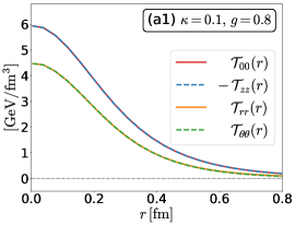
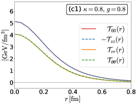
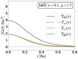
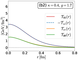
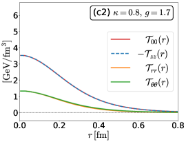
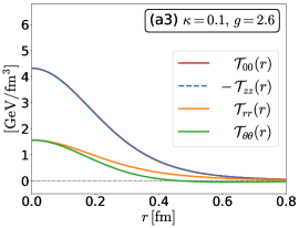
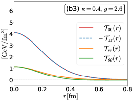
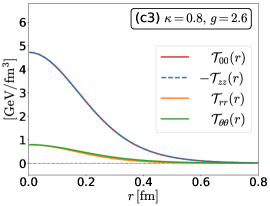
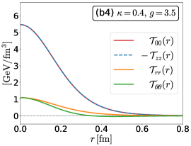
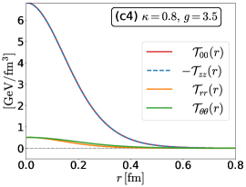
Figure 5: EMT distribution on the mid-plane of the magnetic vortex with $R=0.92$ fm for various combinations of $\kappa$ and $g$. The left, middle, and right panels show the results for $\kappa=0.1$, $0.4$ and $0.8$, respectively, while the value of $g$ is $g=0.8,\,1,7,\,2.6$, and $3.5$ from the top to the bottom.

		0.1	0.4	0.8
0.8	$\xi_{\chi}\,[\mathrm{fm}]$	4.57	1.45	0.84
	$\xi_{A}\,[\mathrm{fm}]$	0.65	0.82	0.94
1.7	$\xi_{\chi}\,[\mathrm{fm}]$	2.15	0.68	0.39
	$\xi_{A}\,[\mathrm{fm}]$	0.30	0.39	0.45
2.6	$\xi_{\chi}\,[\mathrm{fm}]$	1.41	0.45	0.26
	$\xi_{A}\,[\mathrm{fm}]$	0.20	0.25	0.29
3.5	$\xi_{\chi}\,[\mathrm{fm}]$	1.04	0.33	0.19
	$\xi_{A}\,[\mathrm{fm}]$	0.15	0.19	0.22

Table 1: Parameters $\kappa$ and $g$ of the numerical analysis in Fig. 5, and the corresponding values of the correlation lengths $\xi_{\chi}$ and $\xi_{A}$.

We first fix the length of the vortex to be $R=0.92$ fm, the largest length of the flux tube in Ref. Yanagihara:2018qqg , and study the $\kappa$ and $g$ dependence of the EMT distribution on the mid-plane. Shown in Fig. 5 are the EMT distribution on the mid-plane for various combinations of $\kappa$ and $g$. The values of $\kappa$ and $g$ increase along right and lower directions, respectively. The correlation lengths, $\xi_{\chi}$ and $\xi_{A}$, corresponding to each panel are shown in Table 1. With fixed $\kappa$, $\xi_{\chi}$ and $\xi_{A}$ are monotonically decreasing as $g$ becomes larger as in Eq. (3.4). The effect of boundaries thus becomes smaller as $g$ becomes larger. By increasing $\kappa$ with fixed $g$, on the other hand, $\xi_{\chi}$ increases but $\xi_{A}$ is decreases. This behavior comes from the $\kappa$ dependence of $v$ in Eq. (4.23).

From Fig. 5, one finds that the difference between $\mathcal{T}_{rr}(r)$ and $\mathcal{T}_{\theta\theta}(r)$ tends to decrease as $g$ becomes smaller. In particular, one sees that these channels are almost degenerated in the upper two rows, while these channels have a clear separation from $\mathcal{T}_{00}(r)$ and $\mathcal{T}_{zz}(r)$. This result suggests that the degeneracy between $\mathcal{T}_{rr}(r)$ and $\mathcal{T}_{\theta\theta}(r)$ and their separation from $\mathcal{T}_{00}(r)$ and $\mathcal{T}_{zz}(r)$ observed in Ref. Yanagihara:2018qqg can be described by the effects of the boundaries.

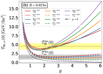
Figure 6: Dependences of $\mathcal{T}_{00}(0)$ and $\mathcal{T}_{rr}(0)$ on $g$ for several values of $\kappa$ at $R=0.46$ fm (left) and $R=0.92$ fm (right). The dash-dotted line shows the contribution from the gauge field $\vec{A}^{D}(r,z)$, Eq. (4.3).

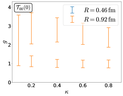
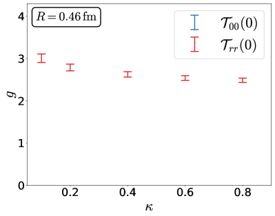
Figure 7: (Left) Range of the parameter $g$ which gives the value of $\mathcal{T}_{00}(0)$ consistent with the lattice result in Ref. Yanagihara:2018qqg . (Right) Range of the parameter $g$ which gives the values of $\mathcal{T}_{00}(0)$ and $\mathcal{T}_{rr}(0)$ consistent with the lattice result in Ref. Yanagihara:2018qqg at $R=0.46$ fm.

$R$ [fm]	$\mathcal{T}_{00}(0)~{}{\rm[GeV/fm^{3}]}$	$\mathcal{T}_{rr}(0)~{}{\rm[GeV/fm^{3}]}$
0.46	13.4 (2)	8.2 (2)
0.92	14.5 (9)	1.5 (7)

Table 2: The values of $\mathcal{T}_{00}(0)$ and $\mathcal{T}_{rr}(0)$ in Ref. Yanagihara:2018qqg for flux tubes with the length $R=0.46$ and $0.92$ fm.

Next, to make the comparison between the vortex in the AH model and lattice results more quantitatively we focus on the absolute values of $\mathcal{T}_{00}(r)$ and $\mathcal{T}_{rr}(r)$ at $r=0$. In Fig. 6 we show the values of $\mathcal{T}_{00}(0)$ and $\mathcal{T}_{rr}(0)$ as functions of $g$ for several values of $\kappa$ at $R=0.46$ and $0.92$ fm. In Fig. 6, we also plot Eq. (4.3) with $n=1$ by the dash-dotted lines. When the condition $R\ll\xi_{A},\xi_{\chi}$ is satisfied, EMT is expected to be dominated by the contribution from the gauge field $\vec{A}^{D}(r,z)$ as discussed in Sec. 4.1. In this case, which is realized in the small $g$ limit, $\mathcal{T}_{00}(0)$ and $\mathcal{T}_{rr}(0)$ should approach as Eq. (4.3). The figure shows that $\mathcal{T}_{00}(0)$ and $\mathcal{T}_{rr}(0)$ have steep rises corresponding to Eq. (4.3) at small $g$. From the figure one also finds that $\mathcal{T}_{00}(0)$ and $\mathcal{T}_{rr}(0)$ go toward degeneracy in this $g$ range.

The horizontal lines in Fig. 6 show the values of $\mathcal{T}_{00}(0)$ and $\mathcal{T}_{rr}(0)$ in Ref. Yanagihara:2018qqg with the errorbars indicated by the shaded region; the numerical values of $\mathcal{T}_{00}(0)$ and $\mathcal{T}_{rr}(0)$ are given in Table 2. We note that the value of $\mathcal{T}_{00}(0)$ used here is obtained from the average $(\mathcal{T}_{00}(0)+\mathcal{T}_{zz}(0))/2$ in Ref. Yanagihara:2018qqg . The value of $g$ with fixed $\kappa$ can be constrained by requiring that $\mathcal{T}_{00}(0)$ of the magnetic vortex reproduces these lattice result. In the left panel of Fig. 7, we show the range of $g$ determined in this way for $R=0.46$ and $0.92$ fm by the bands. The upper and lower bounds of the bands in the panel are the values of $g$ at which $\mathcal{T}_{00}(0)$ of the vortex is the upper and lower bounds of the errorbar of the lattice result. We note that there are two ranges of $g$ for $R=0.92$ fm and $\kappa\geq 0.2$ because of the non-monotonic behavior of $\mathcal{T}_{00}(0)$ as a function of $g$ as shown in Fig. 6. In the result with $R=0.46$ fm, the value of $\mathcal{T}_{00}(0)$ never agrees with the lattice result in Ref. Yanagihara:2018qqg within the statistical error. In the left panel of Fig. 7, therefore, the data corresponding to $\mathcal{T}_{00}(0)$ at $R=0.46$ fm are not shown. This result shows that the vortex solution in the AH model does not have a parameter set which reproduces the EMT distribution of the flux tube in SU(3) YM theory for $0.1<\kappa<0.8$. The same conclusion is also obtained from the right panel of Fig. 7 that shows the range of $g$ constrained by requiring that $\mathcal{T}_{00}(0)$ and $\mathcal{T}_{rr}(0)$ are consistent with the lattice results at $R=0.46$ fm.

6 Summary

In the present study, motivated by the numerical analysis of the $Q\bar{Q}$ system in SU(3) YM theory in Ref. Yanagihara:2018qqg , we investigated the EMT distribution around the flux tube and magnetic vortex. In Sec. 2, using the momentum conservation we have shown that the lattice result on the mid-plane in Ref. Yanagihara:2018qqg is qualitatively inconsistent with an assumption of the translational invariance even at the $Q\bar{Q}$ distance $R=0.92$ fm. We then employed the AH model in Sec. 3 and calculated the EMT distribution on the mid-plane of the magnetic vortex. These results are compared with the lattice result on the basis of the dual superconductor picture Suzuki:1988yq ; Ball:1987cf ; Maedan:1989ju ; Suganuma:1993ps ; Sasaki:1994sa ; Koma:1999sm ; Koma:2003gq . The results obtained with the vortex with finite length suggest that the degeneracy between $\mathcal{T}_{rr}(r)$ and $\mathcal{T}_{\theta\theta}(r)$, and their separation from $\mathcal{T}_{00}(r)$ and $\mathcal{T}_{zz}(r)$, observed in Ref. Yanagihara:2018qqg can be explained qualitatively by the effect of boundaries. However, from the comparison of the absolute values of $\mathcal{T}_{00}(0)$ and $\mathcal{T}_{rr}(0)$, we have shown that the wide range of the parameters in the AH model Eq. (3.1) cannot reproduce the EMT distribution obtained in Ref. Yanagihara:2018qqg simultaneously, although a possibility of the existence of a parameter set in the range $\kappa<0.1$ and $\kappa>0.8$ is not excluded in the present study.

Appendix A Analytic properties

In this appendix, we summarize analytic properties of the magnetic vortex with an infinite length in the AH model at the Bogomol’nyi bound discussed in Refs. Bogomolnyi:1976 .

Throughout this appendix, we use the dimensionless variables $\rho$, $P(\rho)$, and $Q(\rho)$ defined in Eq. (4.14).

The classical vortex solution corresponds to the minimum of Eq. (4.21)

$$\hat{\Sigma}[P,Q] =\int_{0}^{\infty}d\rho\rho\Big{[}\frac{1}{2\rho^{2}}(\partial_{\rho}Q)^{2}+(\partial_{\rho}P)^{2}+\frac{P^{2}Q^{2}}{\rho^{2}}+\kappa^{2}(P^{2}-1)^{2}\Big{]}.$$ (A.1)

with the boundary conditions

$$Q(\rho)\to n,\quad P(\rho)\to 0\qquad\mbox{for }~{}\rho\to 0,$$ (A.2)

$$Q(\rho)\to 0,\quad P(\rho)\to 1\qquad\mbox{for }~{}\rho\to\infty,$$ (A.3)

where we allow for an arbitrary winding number $n$ in this Appendix.

At $\kappa=1/\sqrt{2}$, Eq. (A.1) is rewritten as

$$\hat{\Sigma}[P,Q] =\int_{0}^{\infty}d\rho\rho\Big{[}\frac{1}{2}A_{\pm}(\rho)^{2}+B_{\pm}(\rho)^{2}\Big{]}\mp\int_{0}^{\infty}d\rho\partial_{\rho}(Q(P^{2}-1)).$$ (A.4)

with

$$A_{\pm}(\rho)=\frac{\partial_{\rho}Q}{\rho}\pm(P^{2}-1),\quad B_{\pm}(\rho)=\partial_{\rho}P\pm\frac{PQ}{\rho}.$$ (A.5)

Using these variables, the dimensionless EMT $\hat{\mathcal{T}}_{rr}(\rho)$ and $\hat{\mathcal{T}}_{\theta\theta}(\rho)$ in Eq. (4.15) are given by

$$\hat{\mathcal{T}}_{rr}(\rho)=\frac{1}{4}A_{+}(\rho)A_{-}(\rho)+\frac{1}{2}B_{+}(\rho)B_{-}(\rho),$$ (A.6)

$$\hat{\mathcal{T}}_{\theta\theta}(\rho)=-\frac{1}{4}A_{+}(\rho)A_{-}(\rho)+\frac{1}{2}B_{+}(\rho)B_{-}(\rho).$$ (A.7)

The last term in Eq. (A.4) given by the total derivative is calculated to be

$$\mp\int_{0}^{\infty}d\rho\partial_{\rho}(Q(P^{2}-1))=\mp n$$ (A.8)

with the boundary conditions Eqs. (A.2) and (A.3) and one obtains

$$\hat{\Sigma}[P,Q]=\int_{0}^{\infty}d\rho\rho\Big{[}\frac{1}{2}A_{\pm}(\rho)^{2}+B_{\pm}(\rho)^{2}\Big{]}\mp n.$$ (A.9)

Then, the minimum of Eq. (A.9) is obtained when $A_{\pm}(\rho)=0$ and $B_{\pm}(\rho)=0$ are satisfied for one of the signs of subscript Bogomolnyi:1976 . Assuming that $P(\rho)$ and $Q(\rho)$ are monotonic functions of $\rho$ in the vortex solution, from the boundary conditions one finds that the conditions $A_{+}(\rho)=0$ and $B_{+}(\rho)=0$ are excluded for positive $n$, and hence the vortex solution must satisfy

$$A_{-}(\rho)=B_{-}(\rho)=0.$$ (A.10)

Substituting Eq. (A.10) into Eq. (A.9) one obtains $\hat{\sigma}_{\rm AH}(1/\sqrt{2})=n$ Bogomolnyi:1976 . For $n<0$, $A_{+}(\rho)=0$ and $B_{+}(\rho)=0$ are satisfied, and for an arbitrary $n$ one obtains

$$\hat{\sigma}_{\rm AH}(\kappa)=|n|.$$ (A.11)

at $\kappa=1/\sqrt{2}$.

Finally, substituting Eq. (A.10) into Eqs. (A.6) and (A.7), one easily finds that $\mathcal{T}_{rr}(r)=\mathcal{T}_{\theta\theta}(r)=0$ at $\kappa=1/\sqrt{2}$.

References

- (1) L. D. Landau and E. M. Lifshitz, “The Classical Theory of Fields” (fourth Edition) (Butterworth-Heinemann, 1980).
- (2) R. Yanagihara, T. Iritani, M. Kitazawa, M. Asakawa and T. Hatsuda, Phys. Lett. B 789, 210 (2019) doi:10.1016/j.physletb.2018.09.067 [arXiv:1803.05656 [hep-lat]].
- (3) H. Kawamura and S. Kumano, Phys. Rev. D 89, no. 5, 054007 (2014) doi:10.1103/PhysRevD.89.054007 [arXiv:1312.1596 [hep-ph]].
- (4) S. Kumano, Q. T. Song and O. V. Teryaev, Phys. Rev. D 97, no. 1, 014020 (2018) doi:10.1103/PhysRevD.97.014020 [arXiv:1711.08088 [hep-ph]].
- (5) H. Pagels, Phys. Rev. 144, 1250 (1966). doi:10.1103/PhysRev.144.1250
- (6) M. V. Polyakov and P. Schweitzer, Int. J. Mod. Phys. A 33, no. 26, 1830025 (2018) doi:10.1142/S0217751X18300259 [arXiv:1805.06596 [hep-ph]].
- (7) V. D. Burkert, L. Elouadrhiri and F. X. Girod, Nature 557, no. 7705, 396 (2018). doi:10.1038/s41586-018-0060-z
- (8) P. E. Shanahan and W. Detmold, Phys. Rev. D 99, no. 1, 014511 (2019) doi:10.1103/PhysRevD.99.014511 [arXiv:1810.04626 [hep-lat]].
- (9) P. E. Shanahan and W. Detmold, Phys. Rev. Lett. 122, no. 7, 072003 (2019) doi:10.1103/PhysRevLett.122.072003 [arXiv:1810.07589 [nucl-th]].
- (10) M. Kitazawa, S. Mogliacci, I. Kolbé and W. A. Horowitz, arXiv:1904.00241 [hep-lat].
- (11) H. Suzuki, PTEP 2013, no. 8, 083B03 (2013) [Erratum: PTEP 2015, no. 7, 079201 (2015)] [arXiv:1304.0533 [hep-lat]].
- (12) M. Asakawa et al. [FlowQCD Collaboration], Phys. Rev. D 90, 011501 (2014) [Erratum: Phys. Rev. D 92, no. 5, 059902 (2015)] [arXiv:1312.7492 [hep-lat]].
- (13) H. Makino and H. Suzuki, PTEP 2014, no. 6, 063B02 (2014) [Erratum: PTEP 2015, no. 7, 079202 (2015)] [arXiv:1403.4772 [hep-lat]].
- (14) M. Kitazawa, T. Iritani, M. Asakawa, T. Hatsuda, and H. Suzuki, Phys. Rev. D 94, 114512 (2016) [arXiv:1610.07810 [hep-lat]].
- (15) Y. Taniguchi, S. Ejiri, R. Iwami, K. Kanaya, M. Kitazawa , H. Suzuki, T. Umeda, and N. Wakabayashi, Phys. Rev. D 96, 014509 (2017) [arXiv:1609.01417 [hep-lat]].
- (16) R. Narayanan and H. Neuberger, JHEP 0603, 064 (2006) [hep-th/0601210].
- (17) M. Lüscher, JHEP 1008, 071 (2010) [arXiv:1006.4518 [hep-lat]].
- (18) M. Lüscher and P. Weisz, JHEP 1102, 051 (2011) [arXiv:1101.0963 [hep-th]].
- (19) A. Di Giacomo, M. Maggiore, and S. Olejnik, Nucl. Phys. B 347, 441 (1990).
- (20) G. S. Bali, K. Schilling, and C. Schlichter, Phys. Rev. D 51, 5165 (1995) [hep-lat/9409005].
- (21) C. Michael, Phys. Rev. D 53, 4102 (1996) [hep-lat/9504016].
- (22) A. M. Green, C. Michael and P. S. Spencer, Phys. Rev. D 55, 1216 (1997) [hep-lat/9610011].
- (23) F. Gliozzi, M. Pepe and U.-J. Wiese, Phys. Rev. Lett. 104, 232001 (2010) [arXiv:1002.4888 [hep-lat]].
- (24) H. B. Meyer, Phys. Rev. D 82, 106001 (2010) [arXiv:1008.1178 [hep-lat]].
- (25) P. Cea, L. Cosmai, and A. Papa, Phys. Rev. D 86, 054501 (2012) [arXiv:1208.1362 [hep-lat]].
- (26) N. Cardoso, M. Cardoso, and P. Bicudo, Phys. Rev. D 88, 054504 (2013) [arXiv:1302.3633 [hep-lat]].
- (27) P. Cea, L. Cosmai, F. Cuteri, and A. Papa, JHEP 1606, 033 (2016) [arXiv:1511.01783 [hep-lat]].
- (28) P. Cea, L. Cosmai, F. Cuteri, and A. Papa, Phys. Rev. D 95, 114511 (2017) [arXiv:1702.06437 [hep-lat]].
- (29) G. S. Bali, Phys. Rept. 343, 1 (2001).
- (30) J. Greensite, Lect. Notes. Phys. 821, 1 (2011).
- (31) K. I. Kondo, S. Kato, A. Shibata, and T. Shinohara, Phys. Rept. 579, 1 (2015) [arXiv:1409.1599 [hep-th]].
- (32) R. Yanagihara, M. Kitazawa, T. Iritani, M. Asakawa, T. Hatsuda, oral presentation at the 73th Annual Meeting of Physics Society of Japan, Noda, Japan, Mar. 22, 2019.
- (33) M. Kitazawa, arXiv:1901.06604 [hep-lat].
- (34) S. Nishino, K. I. Kondo, A. Shibata, T. Sasago and S. Kato, arXiv:1903.10488 [hep-lat].
- (35) Y. Nambu, Phys. Rev. D 10, 4262 (1974). doi:10.1103/PhysRevD.10.4262
- (36) G. ’t Hooft, PRINT-75-0836 (UTRECHT).
- (37) S. Mandelstam, Phys. Rept. 23, 245 (1976). doi:10.1016/0370-1573(76)90043-0
- (38) H. B. Nielsen and P. Olesen, Nucl. Phys. B 61, 45 (1973) doi:10.1016/0550-3213(73)90350-7.
- (39) T. Suzuki, Prog. Theor. Phys. 80, 929 (1988). doi:10.1143/PTP.80.929
- (40) J. S. Ball and A. Caticha, Phys. Rev. D 37, 524 (1988). doi:10.1103/PhysRevD.37.524
- (41) S. Maedan, Y. Matsubara and T. Suzuki, Prog. Theor. Phys. 84, 130 (1990). doi:10.1143/PTP.84.130
- (42) H. Kodama, Y. Matsubara, S. Ohno and T. Suzuki, Prog. Theor. Phys. 98, 1345 (1997) doi:10.1143/PTP.98.1345
- (43) G. ’t Hooft, Nucl. Phys. B 190, 455 (1981). doi:10.1016/0550-3213(81)90442-9
- (44) A. S. Kronfeld, G. Schierholz and U. J. Wiese, Nucl. Phys. B 293, 461 (1987). doi:10.1016/0550-3213(87)90080-0
- (45) A. S. Kronfeld, M. L. Laursen, G. Schierholz and U. J. Wiese, Phys. Lett. B 198, 516 (1987). doi:10.1016/0370-2693(87)90910-5
- (46) S. Maedan and T. Suzuki, Prog. Theor. Phys. 81, 229 (1989). doi:10.1143/PTP.81.229
- (47) H. Suganuma, S. Sasaki and H. Toki, Nucl. Phys. B 435, 207 (1995) doi:10.1016/0550-3213(94)00392-R [hep-ph/9312350].
- (48) S. Sasaki, H. Suganuma and H. Toki, Prog. Theor. Phys. 94, 373 (1995). doi:10.1143/PTP.94.373
- (49) H. Ichie, H. Suganuma and H. Toki, Phys. Rev. D 52, 2944 (1995) doi:10.1103/PhysRevD.52.2944 [hep-ph/9502278].
- (50) H. Monden, H. Suganuma, H. Ichie and H. Toki, Phys. Rev. C 57, 2564 (1998) doi:10.1103/PhysRevC.57.2564 [hep-ph/9701271].
- (51) Y. Koma, H. Suganuma and H. Toki, Phys. Rev. D 60, 074024 (1999) doi:10.1103/PhysRevD.60.074024 [hep-ph/9902441].
- (52) Y. Koma, M. Koma, E. M. Ilgenfritz, T. Suzuki and M. I. Polikarpov, Phys. Rev. D 68, 094018 (2003) doi:10.1103/PhysRevD.68.094018 [hep-lat/0302006].
- (53) L. E. Oxman, EPJ Web Conf. 137, 03015 (2017) doi:10.1051/epjconf/201713703015 [arXiv:1704.01989 [hep-th]].
- (54) L. E. Oxman, Phys. Rev. D 98, no. 3, 036018 (2018) doi:10.1103/PhysRevD.98.036018 [arXiv:1805.06354 [hep-th]].
- (55) E. B. Bogomol’nyi, Sov. J. of Nucl. Phys. 24, 449 (1976).
- (56) H. J. de Vega and F. A. Schaposnik, Phys. Rev. D 14, 1100 (1976). doi:10.1103/PhysRevD.14.1100
- (57) A. L. Fetter and J. D. Walecka, “Quantum Theory of Many-Particle Systems” (McGraw-Hill, 1971).
- (58) P. A. M. Dirac, Proc. Roy. Soc. Lond. A 133, no. 821, 60 (1931). doi:10.1098/rspa.1931.0130