Radiative and mechanical feedback into the molecular gas in the Large Magellanic Cloud. II. 30 Doradus

With an aim of probing the physical conditions and excitation mechanisms of warm molecular gas in individual star-forming regions, we performed Herschel SPIRE Fourier Transform Spectrometer (FTS) observations of 30 Doradus in the Large Magellanic Cloud (LMC). In our FTS observations, important far-infrared (FIR) cooling lines in the interstellar medium (ISM), including CO $J$=4–3 to $J$=13–12, [C i] 370 $\mu$m, and [N ii] 205 $\mu$m, were clearly detected. In combination with ground-based CO $J$=1–0 and $J$=3–2 data, we then constructed CO spectral line energy distributions (SLEDs) on $\sim$10 pc scales over a $\sim$60 pc $\times$ 60 pc area and found that the shape of the observed CO SLEDs considerably changes across 30 Doradus, e.g., the peak transition $J_{\rm p}$ varies from $J$=6–5 to $J$=10–9, while the slope characterized by the high-to-intermediate $J$ ratio $\alpha$ ranges from $\sim$0.4 to $\sim$1.8. To examine the source(s) of these variations in CO transitions, we analyzed the CO observations, along with [C ii] 158 $\mu$m, [C i] 370 $\mu$m, [O i] 145 $\mu$m, H₂ 0–0 S(3), and FIR luminosity data, using state-of-the-art models of photodissociation regions (PDRs) and shocks. Our detailed modeling showed that the observed CO emission likely originates from highly-compressed (thermal pressure $P/k_{\rm B}$ $\sim$ 10⁷–10⁹ K cm^-3) clumps on $\sim$0.7–2 pc scales, which could be produced by either ultraviolet (UV) photons (UV radiation field $G_{\rm UV}$ $\sim$ 10³–10⁵ Mathis fields) or low-velocity C-type shocks (pre-shock medium density $n_{\rm pre}$ $\sim$ 10⁴–10⁶ cm^-3 and shock velocity $\varv_{\rm s}$ $\sim$ 5–10 km s^-1). Considering the stellar content in 30 Doradus, however, we tentatively excluded the stellar origin of CO excitation and concluded that low-velocity shocks driven by $\sim$kpc scale processes (e.g., interaction between the Milky Way and the Magellanic Clouds) are likely the dominant source of heating for CO. The shocked CO-bright medium was then found to be warm (temperature $T$ $\sim$ 100–500 K) and surrounded by a UV-regulated low pressure component ($P/k_{\rm B}$ $\sim$ a few (10⁴–10⁵) K cm^-3) that is bright in [C ii] 158 $\mu$m, [C i] 370 $\mu$m, [O i] 145 $\mu$m, and FIR dust continuum emission.

1 Introduction

As a nascent fuel for star formation, molecular gas plays an important role in the evolution of galaxies (e.g., Kennicutt & Evans 2012). The rotational transitions of carbon monoxide (CO) have been the most widely used tracer of such a key component of the interstellar medium (ISM) and in particular enable the examination of the physical conditions of molecular gas in diverse environments (e.g., kinetic temperature $T_{\rm k}$ $\sim$ 10–1000 K and density $n$ $\sim$ 10³–10⁸ cm^-3) thanks to their large range of critical densities.

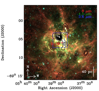
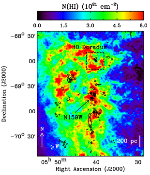
Figure 1: Left: Three-color composite image of 30 Doradus (Spitzer 3.6 $\mu$m, 4.5 $\mu$m, and 8 $\mu$m in blue, green, and red; Meixner et al. 2006). The central star cluster R136 is marked as the red cross, and the FTS coverage is outlined in blue. Additionally, the CO(1–0) integrated intensity from the MAGMA survey (Wong et al. 2011; Sect. 3.4) is overlaid as the black contours with levels ranging from 10% to 90% of the peak (16.6 K km s^-1) in 10% steps. Right: H i column density image from Kim et al. (1998). The MAGMA CO(1–0) integrated intensity is shown as the black contours (10% to 90% of the peak value, 39.5 K km s^-1, in 20% steps), and the coverage of the left image is indicated as the black dashed box. This large H i structure, where 30 Doradus and N159W are located, corresponds to the southeastern H i overdensity region of the LMC (e.g., D’Onghia & Fox 2016).

The diagnostic power of CO rotational transitions has been explored to a greater extent since the advent of the ESA Herschel Space Observatory (Pilbratt et al. 2010). The three detectors on board Herschel, PACS (Photodetector Array Camera and Spectrometer; Poglitsch et al. 2010), SPIRE (Spectral and Photometric Imaging Receiver; Griffin et al. 2010), and HIFI (Heterodyne Instrument for the Far Infrared; de Graauw et al. 2010), provided access to a wavelength window of $\sim$50–670 $\mu$m and enabled the studies of CO spectral line energy distributions (CO SLEDs) up to the upper energy level $J_{\rm u}$ = 50 for Galactic and extragalactic sources including photodissociation regions (PDRs; e.g., Habart et al. 2010; Köhler et al. 2014; Stock et al. 2015; Joblin et al. 2018; Wu et al. 2018), protostars (e.g., Larson et al. 2015), infrared (IR) dark clouds (e.g., Pon et al. 2016), IR bright galaxies (e.g., Rangwala et al. 2011; Kamenetzky et al. 2012; Meijerink et al. 2013; Pellegrini et al. 2013; Papadopoulos et al. 2014; Rosenberg et al. 2014; Schirm et al. 2014; Mashian et al. 2015; Wu et al. 2015), and Seyfert galaxies (e.g., van der Werf et al. 2010; Hailey-Dunsheath et al. 2012; Israel et al. 2014). These studies have revealed the ubiquitous presence of warm molecular gas ($T_{\rm k}$ $\gtrsim$ 100 K) and have proposed various radiative (e.g., ultraviolet (UV) photons, X-rays, and cosmic-rays) and mechanical (e.g., shocks) heating sources for CO excitation. As the dominant contributor to the total CO luminosity of galaxies ($\sim$70%; e.g., Kamenetzky et al. 2017), the warm CO is an important phase of the molecular medium. Understanding its physical conditions and excitation mechanisms would hence be critical to fully assess different molecular reservoirs and their roles in the evolution of galaxies.

While previous Herschel-based studies have considered various types of objects, they have primarily focused on either small-scale Galactic ($\sim$1 pc or smaller) or large-scale extragalactic ($\sim$1 kpc or larger) sources. As recently pointed out by Indriolo et al. (2017), CO SLEDs are affected not only by heating sources, but also by a beam dilution effect, suggesting that it is important to examine a wide range of physical scales to comprehensively understand the nature of warm molecular gas in galaxies. To bridge the gap in the previous studies and provide insights into the excitation mechanisms of warm CO on intermediate scales ($\sim$10–100 pc), we then conducted Herschel SPIRE Fourier Transform Spectrometer (FTS) observations of several star-forming regions in the Large Magellanic Cloud (LMC) (distance of $\sim$50 kpc and metallicity of $\sim$1/2 Z_⊙; e.g., Russell & Dopita 1992; Schaefer 2008). The first of our LMC studies was Lee et al. (2016), where we analyzed Herschel observations of the N159W star-forming region (e.g., Fig. 1 of Lee et al. 2016) along with complementary ground-based CO data at $\sim$10 pc resolution. Specifically, we examined CO transitions from $J$=1–0 to $J$=13–12 ($J$=2–1 not included) over a $\sim$40 pc $\times$ 40 pc area by using the non-LTE (Local Thermodynamic Equilibrium) radiative transfer model RADEX (van der Tak et al. 2007) and found that the CO-emitting gas in N159W is warm ($T_{\rm k}$ $\sim$ 150–750 K) and moderately dense ($n\sim$ a few 10³ cm^-3). To investigate the origin of this warm molecular gas, we evaluated the impact of several radiative and mechanical heating sources and concluded that low-velocity C-type shocks ($\sim$10 km s^-1) provide sufficient energy for CO heating, while UV photons regulate fine-structure lines [C ii] 158 $\mu$m, [C i] 370 $\mu$m, and [O i] 145 $\mu$m. High energy photons and particles including X-rays and cosmic-rays were found not to be significant for CO heating.

Table 1: Spectral line and dust continuum data in our study.

Transition	Rest wavelength	$E_{\rm u}^{a}$	FWHMb	$\sigma_{\rm s,med}^{c,e,f}$	$\sigma_{\rm f,med}^{d,e,f}$	Referenceg
	($\mu$m)	(K)	(′′)	(10-11 W m-2 sr-1)	(10-11 W m-2 sr-1)
12CO $J$=1–0	2600.8	6	45	0.1	0.1	(1)
12CO $J$=3–2	867.0	33	22	2.2	5.1	(2)
12CO $J$=4–3	650.3	55	42	24.0	26.5	(3)
12CO $J$=5–4	520.2	83	34	15.9	20.7	(3)
12CO $J$=6–5	433.6	116	29	9.2	16.7	(3)
12CO $J$=7–6	371.7	155	33	7.4	18.4	(3)
12CO $J$=8–7	325.2	199	33	18.7	25.3	(3)
12CO $J$=9–8	289.1	249	19	25.2	30.2	(3)
12CO $J$=10–9	260.2	304	18	27.6	30.6	(3)
12CO $J$=11–10	236.6	365	17	28.7	32.2	(3)
12CO $J$=12–11	216.9	431	17	26.6	30.3	(3)
12CO $J$=13–12	200.3	503	17	39.8	43.0	(3)
[C i] ${}^{3}P_{1}$–${}^{3}P_{0}$	609.1	24	38	28.3	29.2	(3)
[C i] ${}^{3}P_{2}$–${}^{3}P_{1}$	370.4	62	33	7.0	7.9	(3)
[C ii] ${}^{2}P_{3/2}$–${}^{2}P_{1/2}$	157.7	91	12	294.6	8092.0	(4)
[O i] ${}^{3}P_{0}$–${}^{3}P_{1}$	145.5	327	12	110.2	788.0	(4)
[N ii] ${}^{3}P_{1}$–${}^{3}P_{0}$	205.2	70	17	43.6	99.0	(3)
H2 0–0 S(3)	9.7	2504	6	–	1036.0	(3,5)
FIR	60–200	–	42	–	2.9 $\times$ 106	(3,4)

^(a) Upper level energy. ^(b) Angular resolution of the original data. ^(c) Median $\sigma_{\rm s}$ (statistical 1$\sigma$ uncertainty) on 42^′′ scales. ^(d) Median $\sigma_{\rm f}$ (final 1$\sigma$ uncertainty; statistical and calibration errors added in quadrature) on 42^′′ scales. ^(e) CO(1–0) is exceptionally on 45^′′ scales. ^(f) All pixels are considered. ^(g) (1) Wong et al. (2011); (2) Minamidani et al. (2008); (3) This work; (4) Chevance et al. (2016); (5) Indebetouw et al. (2009)

In this paper, we extend our previous analyses to 30 Doradus (or 30 Dor), the most extreme starburst in the Local Universe. 30 Doradus harbors more than 1000 massive young stars, e.g., OB-type and Wolf-Rayet (W-R) stars (Doran et al. 2013), and emits $\sim$500 times more ionizing photons than the Orion Nebula (Pellegrini et al. 2010), producing a giant H ii region. In particular, 30 Doradus is primarily powered by the central super star cluster R136, which has an extremely high stellar surface density ($\gtrsim$ 10⁷ M_⊙ pc^-3; e.g., Selman & Melnick 2013) along with the most massive stars known ($\gtrsim$ 150 M_⊙; e.g., Crowther et al. 2010). R136 is surrounded by vast cavities and bubble-like structures, which were likely created by strong stellar winds and supernova explosions (SNe) with a total energy of $\sim$10⁵² erg (e.g., Chu & Kennicutt 1994; Townsley et al. 2006a). All in all, these extraordinary star formation activities make 30 Doradus an ideal laboratory for examining the impact of radiative and mechanical feedback into the surrounding ISM. In Fig. 1, we show 30 Doradus and its surrounding environment (H i overdensity region where 30 Doradus and N159W are located) in several tracers of gas and dust.

This paper is organized as follows. In Sect. 2, we provide a summary on recent studies of 30 Doradus that are most relevant to our work. In Sects. 3 and 4, we present the multi-wavelength datasets used in our study and describe the spatial distribution of CO and [C i] emission, as well as the observed CO SLEDs. In Sects. 5 and 6, we then employ state-of-the-art theoretical models of PDRs and shocks to examine the physical conditions and excitation mechanisms of CO in 30 Doradus. Finally, we summarize the results from our study in Sect. 7.

2 Characteristics of 30 Doradus

As noted in Sect. 1, 30 Doradus is one of the best-studied star-forming regions. In this section, we summarize recent studies on 30 Doradus that are most relevant to our work.

2.1 Stellar content

When it comes to stellar feedback, massive young stars are considered to be a major player; their abundant UV photons create H ii regions and PDRs, while their powerful stellar winds sweep up the surrounding ISM into shells and bubbles. The latest view on the massive young stars in 30 Doradus has been offered from the VLT-FLAMES Tarantula Survey (Evans et al. 2011), and we focus here on Doran et al. (2013) where the first systematic census of hot luminous stars was presented. In Doran et al. (2013), 1145 candidate hot luminous stars were identified based on UBV band photometry, and $\sim$500 of these stars were spectroscopically confirmed (including 469 OB-type stars and 25 W-R stars). The total ionizing and stellar wind luminosities were then estimated to be $\sim$10⁵² photons s^-1 and $\sim$2 $\times$ 10³⁹ erg s^-1 respectively, and $\sim$75% of these luminosities were found to come from the inner 20 pc of 30 Doradus. This implies that stellar feedback is highly concentrated in the central cluster R136, where one third of the total W-R stars reside along with a majority of the most massive O-type stars. As for the age of stellar population, Doran et al. (2013) showed that the ionizing stars in 30 Doradus span multiple ages: mostly 2–5 Myr with an extension beyond 8 Myr.

2.2 Properties of the neutral gas

The impact of UV photons on the neutral gas in 30 Doradus was recently studied in detail by Chevance et al. (2016). The authors focused on Herschel PACS observations of traditional PDR tracers, including [C ii] 158 $\mu$m and [O i] 63 $\mu$m and 145 $\mu$m, and found that [C ii] and [O i] mostly arise from the neutral medium (PDRs), while [O i] 63 $\mu$m is optically thick. The observed [C ii] 158 $\mu$m and [O i] 145 $\mu$m were then combined with an image of IR luminosity to estimate the thermal pressure of $\sim$(1–20) $\times$ 10⁵ K cm^-3 and the UV radiation of $\sim$(1–300) $\times$ 10² Mathis fields (Mathis et al. 1983) via Meudon PDR modeling (Le Petit et al. 2006) on 12^′′ scales ($\sim$3 pc). In addition, the three-dimensional structure of PDRs was inferred based on a comparison between the stellar UV radiation field and the incident UV radiation field determined from PDR modeling: PDR clouds in 30 Doradus are located at a distance of $\sim$20–80 pc from the central cluster R136.

As for the molecular ISM in 30 Doradus, Indebetouw et al. (2013) provided the sharpest view ever ($\sim$2^′′ or $\sim$0.5 pc scales) based on ALMA CO(2–1), ¹³CO(2–1), and C¹⁸O(2–1) observations of the 30Dor-10 cloud (Johansson et al. 1998). The main findings from their study include: (1) CO emission mostly arises from dense clumps and filaments on $\sim$0.3–1 pc scales; (2) Interclump CO emission is minor, suggesting that there is considerable photodissociation of CO molecules by UV photons penetrating between the dense clumps; (3) The mass of CO clumps does not change very much with distance from R136. More excited CO lines in 30 Doradus (up to $J$=6–5) were recently analyzed by Okada et al. (2019), and we discuss this work in detail in Appendix E.

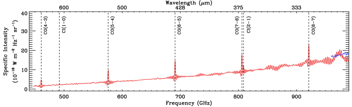
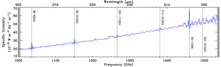
Figure 2: Point source calibrated spectra from two central detectors, SLWC3 (red) and SSWD4 (blue). These spectra are from the first jiggle position of the Obs. ID = 1342219550, and the locations of the two detectors are shown as the yellow and orange crosses in Fig. 3. Additionally, the spectral lines observed with the SPIRE FTS are indicated as the black dashed lines. Note that no further data processing (e.g., baseline subtraction and smoothing) was done for the spectral lines here, which are at their original angular resolutions (e.g., Table 1).

Figure 3: CO(7–6) integrated intensity image (FWHM = 42^′′; pixel size = 30^′′). In our FTS observations, CO(7–6) is one of the brightest and most sensitive transitions (Table 1; Sect. 4). Over the grayscale image, the spectrum of each pixel is overlaid, whose $x$- and $y$-axis ranges (in GHz and 10^-18 W m^-2 Hz^-1 sr^-1) are indicated in the top left corner with an example spectrum. This spectrum is from the pixel that was observed with the two central detectors SLWC3 and SSWD4 (yellow and orange crosses) of the first jiggle observation of the Obs. ID = 1342219550. The spectra in red and blue represent detections and non-detections based on our threshold of $S/N_{\rm s}$ = 5 (statistical signal-to-noise ratio; Sect. 4.1).

2.3 High energy photons

30 Doradus has also been known as a notable source of high energy photons. For example, Townsley et al. (2006a, b) presented Chandra X-ray observations of 30 Doradus, where a convoluted network of diffuse structures (associated with superbubbles and supernova remnants (SNRs)), as well as $\sim$100 point sources (associated with O-type stars and W-R stars), were revealed. Thanks to the high spatial and spectral resolutions of the Chandra observations, the authors were able to investigate the properties of the X-ray-emitting hot plasma in detail, estimating the temperature of (3–9) $\times$ 10⁶ K and the surface brightness of (3–130) $\times$ 10³¹ erg s^-1 pc^-2. In addition, Fermi $\gamma$-ray observations recently showed that 30 Doradus is the brightest source in the LMC with an emissivity of $\sim$3 $\times$ 10^-26 photons s^-1 sr^-1 per hydrogen atom (Abdo et al. 2010). All in all, the presence of high energy photons in 30 Doradus suggests that strong stellar winds and SNe have injected a large amount of mechanical energy into the surrounding ISM, driving shocks and accelerating particles.

3 Data

In this section, we present the data used in our study. Some of the main characteristics of the datasets, including rest wavelengths, angular resolutions, and sensitivities, are listed in Table 1.

3.1 Herschel SPIRE spectroscopic data

30 Doradus was observed with the SPIRE FTS in the high spectral resolution, intermediate spatial sampling mode (Obs. IDs: 1342219550, 1342257932, and 1342262908). The FTS consists of two bolometer arrays, SPIRE Long Wavelength (SLW) and SPIRE Short Wavelength (SSW), which cover the wavelength ranges of 303–671 $\mu$m and 194–313 $\mu$m. Depending on wavelength, the FTS beam size ranges from 17^′′ to 42^′′ (corresponding to 4–10 pc at the distance of the LMC; Makiwa et al. 2013; Wu et al. 2015). The SLW and SSW comprise 19 and 37 hexagonally packed detectors, which cover approximately 3^′ $\times$ 3^′. In the intermediate spatial sampling mode, these bolometer arrays are moved in a four-point jiggle with one beam spacing, resulting in sub-Nyquist-sampled data. Note that spectral lines are not resolved in our observations due to the insufficient frequency resolution of $\Delta f$ = 1.2 GHz (corresponding to the velocity resolution of $\Delta\varv$ $\sim$ 230–800 km s^-1 across the SLW and SSW).

To derive integrated intensity images and their uncertainties, we essentially followed Lee et al. (2016) and Wu et al. (2015) and summarize our procedure here. First of all, we processed the FTS data using the Herschel Interactive Processing Environment (HIPE) version 11.0, along with the SPIRE calibration version 11.0 (Fulton et al. 2010; Swinyard et al. 2014). As an example, the processed spectra from two central SLW and SSW detectors are presented in Fig. 2, with the locations of the spectral lines observed with the SPIRE FTS. We then performed line measurement of point source calibrated spectra for each transition, where a linear combination of parabola and sinc functions was adopted to model the continuum and the emission line. The continuum subtracted spectra were eventually projected onto a 5^′ $\times$ 5^′ common grid with a pixel size of 15^′′ to construct a spectral cube. Finally, the integrated intensity ($I_{\rm CO}$, $I_{\rm CI}$, or $I_{\rm NII}$) was derived by carrying out line measurement of the constructed cube, and its final 1$\sigma$ uncertainty ($\sigma_{\rm f}$) was estimated by summing two sources of error in quadrature, $\sigma_{\rm f}$ = $\sqrt{\sigma_{\rm s}^{2}+\sigma_{\rm c}^{2}}$, where $\sigma_{\rm s}$ is the statistical error derived from line measurement and $\sigma_{\rm c}$ is the calibration error of 10% (SPIRE Observers’ Manual).

Throughout our study, the FTS data were frequently combined with other tracers of gas and dust. To compare the different datasets at a common angular resolution, we then smoothed the FTS images to 42^′′, which corresponds to the FWHM of the FTS CO(4–3) observations, by employing the kernels from Wu et al. (2015). These kernels were created based on the fitting of a two-dimensional Hermite-Gaussian function to the FTS beam profile, taking into account the complicated dependence on wavelength. In addition, the smoothed images were rebinned to have a final pixel size of 30^′′, which roughly corresponds to the jiggle spacing of the SLW observations. We present the resulting integrated intensity maps in Fig. 3 and Appendix A and refer to Lee et al. (2016) and Wu et al. (2015) for full details on the data reduction and map-making procedures. Line detections in our FTS observations are discussed in Sect. 4.1.

We note that high resolution spectra of CO(4–3), CO(7–6), and [C i] 370 $\mu$m ($\sim$25^′′–40^′′) were previously obtained for 30 Doradus by Pineda et al. (2012) with the NANTEN2 telescope. The authors performed the observations as a single pointing toward ($\alpha$, $\delta$)_J2000 = (05^h38^m48.6^s, $-69^{\circ}$04^′43.2^′′), and we found that the NANTEN2-to-FTS ratios of the integrated intensities for this position are $\lesssim$ 1.2, suggesting that our intensity measurements are consistent with Pineda et al. (2012) within 1$\sigma$ uncertainties.

3.2 Herschel PACS spectrosopic data

Following Lee et al. (2016), we used PACS [C ii] 158 $\mu$m and [O i] 145 $\mu$m data of 30 Doradus. These data were first presented in Chevance et al. (2016), and we here provide a brief summary on the observations and data reduction. Note that [O i] 63 $\mu$m was not used for our study, since the line is optically thick throughout the mapped region (e.g., [O i] 145 $\mu$m-to-[O i] 63 $\mu$m ratio $>$ 0.1; Tielens & Hollenbach 1985; Chevance et al. 2016).

30 Doradus was mapped with the PACS spectrometer in the unchopped scan mode (Obs. IDs: 1342222085 to 1342222097 and 1342231279 to 1342231285). As an integral field spectrometer, the PACS consists of 25 (spatial) $\times$ 16 (spectral) pixels and covers 51–220 $\mu$m with a field-of-view of 47^′′ $\times$ 47^′′ (Poglitsch et al. 2010). The [C ii] 158 $\mu$m and [O i] 145 $\mu$m fine-structure lines were observed in 31 and 11 raster positions, covering approximately 4^′ $\times$ 5^′ over the sky. The beam size of the spectrometer at 160 $\mu$m is 12^′′ (PACS Observers’ Manual).

The obtained observations were reduced using the HIPE version 12.0 (Ott 2010) from Level 0 to Level 1. The reduced cubes were then processed with PACSman (Lebouteiller et al. 2012) to derive integrated intensity maps. In essence, each spectrum was modeled with a combination of polynomial (baseline) and Gaussian (emission line) functions, and the measured line fluxes were projected onto a common grid with a pixel size of 3^′′. The final 1$\sigma$ uncertainty in the integrated intensity was then estimated by adding the statistical error from line measurement/map projection and the calibration error of 22% in quadrature. For details on the observations, as well as the data reduction and map-making procedures, we refer to Lebouteiller et al. (2012), Cormier et al. (2015), and Chevance et al. (2016).

In our study, the original PACS images were smoothed and rebinned to match the FTS resolution (42^′′) and pixel size (30^′′). This smoothing and rebinning procedure resulted in a total of 13 common pixels to work with (e.g., Fig. 7; mainly limited by the small coverage of the [O i] 145 $\mu$m data), over which [C ii] 158 $\mu$m and [O i] 145 $\mu$m were clearly detected with $S/N_{\rm s}$ $\gg$ 5.

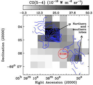
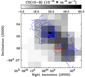
Figure 4: Comparison between CO ($J$=5–4 and $J$=10–9 on the left and right plots) and [C ii] 158 $\mu$m (blue contours). The PACS [C ii] 158 $\mu$m data at the original resolution of 12^′′ are overlaid with levels ranging from 20% to 90% of the peak (2.2 $\times$ 10^-6 W m^-2 sr^-1) in 10% steps. The location of the R136 cluster is indicated as the red circle. Note that the grayscale bar goes below zero simply to show the pixels with low intensities.

3.3 Spitzer IRS H₂ data

In addition, we made use of Spitzer InfraRed Spectrograph (IRS) observations of H₂ 0–0 S(3) in 30 Doradus. These observations were initially presented in Indebetouw et al. (2009), and we re-processed them as follows mainly to match the FTS resolution and pixel size. First, Basic Calibrated Data (BCD) products were downloaded from the Spitzer Heritage Archive (SHA), and exposures were cleaned with IRSclean and combined using SMART (Higdon et al. 2004; Lebouteiller et al. 2010). The data were then imported into CUBISM (Smith et al. 2007) for further cleaning and building a calibrated data cube with pixel sizes of 2^′′ and 5^′′ for the Short-Low (SL) and Long-Low (LL) modules.

To produce a H₂ 0–0 S(3) map, we performed a Monte Carlo simulation where 100 perturbed cubes were created based on the calibrated data cube. These cubes were then convolved and resampled to have a resolution of 42^′′ and a pixel size of 30^′′, and spectral line fitting was performed using LMFIT (Newville et al. 2014) for each cube. Finally, the line flux and associated uncertainty were calculated for each pixel using the median and median absolute deviation of the 100 measured flux values. While the resulting H₂ map is as large as the FTS CO maps, we found that the observations were not sensitive: only five pixels have detections with $S/N_{\rm s}$ $\sim$ 5.

3.4 Ground-based CO data

We complemented our FTS CO observations with ground-based CO(1–0) and (3–2) data. The CO(1–0) data were taken from the MAGellanic Mopra Assessment (MAGMA) survey (Wong et al. 2011), where the 22-m Mopra telescope was used to map CO(1–0) in the LMC on 45^′′ scales. Meanwhile, the CO(3–2) data were obtained by Minamidani et al. (2008) on 22^′′ scales using the 10-m Atacama Submillimeter Telescope Experiment (ASTE) telescope. For both datasets, the final uncertainties in the integrated intensities were estimated in a similar manner as we did for our FTS CO observations: adding the statistical error derived from the root-mean-square (rms) noise per channel and the calibration error (25% and 20% for CO(1–0) and CO(3–2) respectively; Lee et al. 2016) in quadrature. We smoothed and rebinned the CO(1–0) and CO(3–2) maps to match the FTS data, leading to 31 and 26 pixels to work with respectively. Among these pixels, a majority (22 and 25 pixels for CO(1–0) and CO(3–2) respectively) had clear detections with $S/N_{\rm s}$ $>$ 5 (e.g., Fig. 5).

3.5 Derived dust and IR continuum properties

Finally, we used the dust and IR continuum properties of 30 Doradus that were first estimated by Chevance et al. (2016) at 12^′′ resolution based on the dust spectral energy distribution (SED) model of Galliano (2018). The Galliano (2018) SED model employs the hierarchical Bayesian approach and considers realistic optical properties, stochastic heating, and the mixing of physical conditions in observed regions. For our analyses, we essentially followed Chevance et al. (2016) and constrained the far-IR luminosity (60–200 $\mu$m; $L_{\rm FIR}$) and $V$-band dust extinction ($A_{V}$) over the FTS coverage on 42^′′ scales. In our spatially resolved modeling of dust SEDs covering mid-IR to sub-mm, the amorphous carbon (AC) composition was considered along with the following free parameters: the total dust mass ($M_{\rm dust}$), PAH (polycyclic aromatic hydrocarbon)-to-dust mass ratio ($f_{\rm PAH}$), index for the power-law distribution of starlight intensities ($\alpha_{U}$), lower cut-off for the power-law distribution of starlight intensities ($U_{\rm min}$), range of starlight intensities ($\Delta U$), and mass of old stars ($M_{\rm star}$). For details on our dust SED modeling, we refer to Galliano (2018).

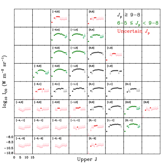
Figure 5: CO SLEDs of 30 Doradus. Here each CO SLED was constructed by using all available CO transitions from $J_{\rm u}$ = 1 to 13 for an individual data point in 30^′′ size. To indicate a location relative to the pixel that is closest to R136, a pair of numbers is shown in the top left corner of each pixel, e.g., [0,0] corresponds to ($\alpha$, $\delta$)_J2000 = (05^h38^m42^s, $-69^{\circ}$05^′53^′′). In addition, the circles and error bars (too small to be visible in many cases) show the measured intensities and 1$\sigma$ uncertainties for detections, while the downward arrows represent the upper limits based on $S/N_{\rm s}$ = 5 for non-detections. Finally, the CO SLEDs are presented in different colors depending on the transition they peak ($J_{\rm p}$): black ($J_{\rm p}$=9–8 or 10–9), green (6–5 $\leq$ $J_{\rm p}$ $<$ 9–8), and red (uncertain $J_{\rm p}$ due to many non-detections). The non-detections are then shown in lighter shades (gray, light green, and pink) to distinguish them from the detections.

4 Results

In this section, we mainly discuss the observed properties of the FTS lines, with a particular emphasis on CO and [C i] emission. The spectra and integrated intensity images of the FTS lines are presented in Fig. 3 and Appendix A.

4.1 Spatial distribution of CO and [C i] emission

Following Lee et al. (2016), we consider spectra with $S/N_{\rm s}$ (statistical signal-to-noise ratio; integrated intensity divided by $\sigma_{\rm s}$) $>$ 5 as detections and group CO transitions into three categories: low-$J$ for $J_{\rm u}\leq 5$, intermediate-$J$ for $6\leq J_{\rm u}\leq 9$, and high-$J$ for $J_{\rm u}\geq 10$. In our FTS observations, all CO transitions from $J$=4–3 to $J$=13–12, as well as [C i] 370 $\mu$m, were clearly detected. The sensitivity at $\sim$500 GHz, on the other hand, was not good enough for [C i] 609 $\mu$m to be detected.

In general, we found that CO ($J$=1–0 to 13–12; $J$=2–1 not included) and [C i] 370 $\mu$m emission lines are distributed along the northern and southern lobes around R136, with primary and secondary peaks at ($\alpha$, $\delta$)_J2000 $\sim$ (05^h38^m51^s, $-69^{\circ}$04^′38^′′) and (05^h38^m38^s, $-69^{\circ}$06^′08^′′) (e.g., Fig 4). This overall morphology is similar to that of PDR tracers, such as [C ii] 158 $\mu$m, [O i] 145 $\mu$m, and PAH emission (Chevance et al. 2016). A close examination, however, revealed that detailed distributions are slightly different between the transitions. For example, the region between the northern and southern lobes, ($\alpha$, $\delta$)_J2000 $\sim$ (05^h38^m45^s, $-69^{\circ}$05^′30^′′), becomes bright in intermediate- and high-$J$ CO emission, resulting in the declining correlation between CO lines and fine-structure lines. To be specific, we found that the Spearman rank correlation coefficient remains high ($\rho\sim$ 0.8–0.9) for [C ii] 158 $\mu$m and CO from $J$=1–0 to 8–7 ($J$=2–1 not included), while being low for $J$=9–8 and 10–9 ($\rho$ = 0.4 and 0.1). [C i] 370 $\mu$m was found to be strongly correlated with [C ii] 158 $\mu$m ($\rho$ = 0.9). For these estimates, we only considered detections and the transitions with sufficient number of detections. The decreasing correlation between [C ii] 158 $\mu$m and CO mainly results from the mid-region becoming bright in intermediate- and high-$J$ CO lines, indicating the spatial variations in CO SLEDs (Sect. 4.2). To illustrate this result, we show CO $J$=5–4 and 10–9 along with [C ii] 158 $\mu$m in Fig. 4.

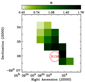
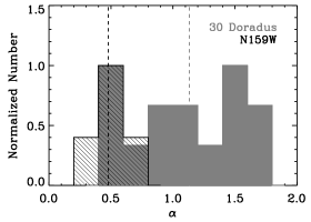
Figure 6: Left: High-to-intermediate-$J$ CO ratio ($\alpha$) for 30 Doradus. For the derivation of $\alpha$, 25 pixels were masked since they have non-detections for the required transitions. The location of R136 is also indicated as the red circle. Right: Comparison of $\alpha$ between 30 Doradus (gray, solid) and N159W (black, hatched). The $\alpha$ values of N159W were calculated by applying Eq. (1) to the data from Lee et al. (2016), and the median value of each histogram is shown as the dashed line. For both 30 Doradus and N159W, the $\alpha$ values are on 42^′′ scales.

4.2 Observed CO SLEDs

The observed CO SLEDs of 30 Doradus are presented in Fig. 5. To construct these CO SLEDs, we first combined the FTS integrated intensity images with the ground-based CO(1–0) and (3–2) data at the common resolution of 42^′′. We then used different colors to indicate the CO SLEDs with different peak transitions (black, green, and red for $J_{\rm p}\geq$ 9–8, $J_{\rm p}$ $<$ 9–8, and uncertain $J_{\rm p}$; $J_{\rm p}$ = transition where a CO SLED peaks) and marked the location of each pixel relative to R136.

Fig. 5 clearly shows that the shape of the CO SLEDs changes over the mapped region of 4^′ $\times$ 4^′ ($\sim$60 pc $\times$ 60 pc). For example, the majority (12 out of the total 21 pixels with certain $J_{\rm p}$) peak at $J$=9–8 or 10–9, while some have 6–5 $\leq$ $J_{\rm p}$ $<$ 9–8. In addition, the slope of the CO SLEDs varies substantially. To quantify the variation in the slopes, we then defined the high-to-intermediate-$J$ CO ratio ($\alpha$) as follows,

$$\alpha=\frac{I_{\rm CO}(J\!=\!9\!-\!8)+I_{\rm CO}(J\!=\!10\!-\!9)+I_{\rm CO}(J\!=\!11\!-\!10)}{I_{\rm CO}(J\!=\!5\!-\!4)+I_{\rm CO}(J\!=\!6\!-\!5)+I_{\rm CO}(J\!=\!7\!-\!6)},$$ (1)

and estimated $\alpha$ on a pixel-by-pixel basis (Fig. 6 Left). 25 pixels were additionally masked in the process since they have non-detections for the required transitions. Note that we did not adopt the “high-$J$ slope”, $\Delta I_{\rm CO,norm}\!=\![I_{\rm CO}(J_{\rm p}\!+\!3)\!-I_{\rm CO}(J_{\rm p})]\!/\!I_{\rm CO}(J_{\rm p})$, the parameter Lee et al. (2016) used to characterize the observed CO SLEDs of N159W. This is because the high-$J$ slope, which measures a slope only beyond $J_{\rm p}$, was found not to capture the more general shape around the peak of the CO SLEDs, e.g., our [$-1$,4] and [0,0] pixels would have comparable high-$J$ slopes of $-$0.24 despite their distinctly different CO SLEDs (the peak for [0,0] is much broader). In addition, we note that our $\alpha$ parameter is only slightly different from what Rosenberg et al. (2015) adopted to classify 29 (U)LIRGs: we used CO $J$=9–8, 10–9, and 11–10 for the high-$J$ CO contribution instead of CO $J$=11–10, 12–11, and 13–12 to better reflect the properties of the CO SLEDs observed in 30 Doradus, as well as to maximize the number of available transitions for the derivation of $\alpha$.

We found that the derived $\alpha$ peaks around R136 with a value of 1.5–1.8 and decreases radially down to $\sim$0.4, implying that the relative contribution of high-$J$ CO lines increases toward R136. Compared to N159W, another massive star-forming region in the LMC, 30 Doradus shows systematically higher $\alpha$ (Fig. 6 right). Specifically, the $\alpha$ values of N159W mostly trace the lower range of the 30 Doradus histogram with a factor of two lower median value ($\sim$0.5 vs. $\sim$1.1). This result indicates that the two regions have markedly different CO SLEDs, and we will revisit the shape of CO SLEDs as a probe of heating sources in Sect. 6.3.

The varying $\alpha$, as well as the different $J_{\rm p}$ for the individual pixels, suggest that the properties of the CO-emitting gas change across 30 Doradus on 42^′′ or 10 pc scales. For example, the peak transition and slope of the CO SLEDs depend on the gas density and temperature, while the CO column density affects the overall line intensities. In the next sections, the physical conditions and excitation sources of the CO-emitting gas will be examined in a self-consistent manner based on state-of-the-art models of PDRs and shocks. In addition, the impact of high energy photons and particles, e.g., X-rays and cosmic-rays, on CO emission will also be assessed.

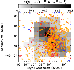
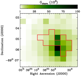
Figure 7: Left: UV sources overlaid on the CO(9–8) integrated intensity image. $\sim$1.3 $\times$ 10⁴ stars we used for the derivation of $G_{\rm stars}$ (right; Appendix B for details) are presented here with different symbols depending on the stellar effective temperature $T_{\rm eff}$: $T_{\rm eff}$ $\geq$ 3 $\times$ 10⁴ K (1406 stars as the red crosses; mostly O-type or W-R), 10⁴ K $\leq$ $T_{\rm eff}$ $<$ 3 $\times$ 10⁴ K (9807 stars as the orange circles; mostly B-type) and $T_{\rm eff}$ $<$ 10⁴ K (2116 stars as the blue triangles). The location of R136 is also indicated as the black circle. Right: Stellar UV radiation field $G_{\rm stars}$ on the plane of R136 (in units of 10³ Mathis fields). The pixels used for our PDR modeling are outlined in red.

5 Excitation sources for CO

5.1 Radiative source: UV photons

Far-UV ($E$ = 6–13.6 eV) photons from young stars have a substantial influence on the thermal and chemical structures of the surrounding ISM. As for gas heating, the following two mechanisms are then considered important: (1) photo-electric effect on large PAH molecules and small dust grains (far-UV photons absorbed by PAH molecules and grains create free electrons, which carry off excess kinetic energy of several eVs; e.g., Bakes & Tielens 1994; Weingartner & Draine 2001; Weingartner et al. 2006) and (2) far-UV pumping of H₂ molecules (far-UV pumped H₂ molecules mostly fluoresce back to a vibrational state in the electronic ground state, and these vibrationally excited H₂ molecules can heat the gas through collisional de-excitation; e.g., Sternberg & Dalgarno 1989; Burton et al. 1990).

As the most extreme star-forming region in the Local Group of galaxies, 30 Doradus hosts numerous massive stars producing an ample amount of UV photons (Sect. 2.1). In Fig. 7, such UV sources are overlaid on the integrated intensity image of CO(9–8), the transition where most of the observed CO SLEDs peak (Sect. 4.2). The strong concentration of the hot luminous stars in the central cluster R136 is particularly striking. In addition, we present the UV radiation field on the plane of R136 (calculated by utilizing published catalogs of massive stars; Appendix B for details) in Fig. 7. This UV radiation field $G_{\rm stars}$ on the plane of R136 ranges from $\sim$8 $\times$ 10² to $\sim$4 $\times$ 10⁵ Mathis fields (its peak coincides well with R136) and can be considered as the maximum incident radiation field we would expect, since no absorption was taken into account. In the following sections, we evaluate the influence of the intense UV radiation field in 30 Doradus on CO emission by performing PDR modeling.

5.1.1 Meudon PDR model

For our purpose, we used the Meudon PDR model (Le Petit et al. 2006). This one-dimensional stationary model essentially computes the thermal and chemical structures of a plane-parallel slab of gas and dust illuminated by a radiation field by solving radiative transfer, as well as thermal and chemical balance. A chemical network of 157 species and 2916 reactions was adopted, and in particular H₂ formation was modeled based on the prescription by Le Bourlot et al. (2012), which considers the Langmuir-Hinshelwood and Eley-Rideal mechanisms. While more sophisticated treatment of H₂ formation taking into account dust temperature fluctuations is important, as demonstrated by Bron et al. (2014, 2016), we did not use this detailed model due to computing time reasons. Consideration of stochastic fluctuations in the dust temperature could increase H₂ formation in UV-illuminated regions, resulting in brighter emission of H₂ and other molecules that form once H₂ is present, e.g., CO. As for the thermal structure of the slab, the gas temperature was calculated in the stationary state considering the balance between heating and cooling. The main heating processes were the photo-electric effect on grains and H₂ collisional de-excitation, and cooling rates were then derived by solving the non-LTE populations of main species such as C⁺, C, O, CO, etc.

Table 2: Input parameters tailored for 30 Doradus^a.

Parameter	Value
Metallicity ($Z$)	0.5 $Z_{\odot}$
Dust-to-gas mass ratio ($M_{\rm dust}/M_{\rm gas}$)	5 $\times$ 10-3
PAH fraction ($f_{\rm PAH}$)	1%
Element	Gas phase abundance
	(log${}_{10}(n(X)/n({\rm H}))$)
He	$-1.05$
C	$-4.30$
N	$-4.91$
O	$-3.75$
Ne	$-4.36$
Si	$-5.51$
S	$-5.32$

^(a) See Chevance et al. (2016) for details on these parameters.

In the Meudon PDR model, the following three parameters play an important role in controlling the structure of a PDR: (1) dust extinction $A_{V}$, (2) thermal pressure $P$, and (3) radiation field $G_{\rm UV}$. Specifically, the radiation field has the shape of the interstellar radiation field in the solar neighborhood as measured by Mathis et al. (1983), and its intensity scales with the factor $G_{\rm UV}$ ($G_{\rm UV}$ = 1 corresponds to the integrated energy density of 6.0 $\times$ 10^-14 erg cm^-3 for $E$ = 6–13.6 eV). For our modeling of 30 Doradus, a plane-parallel slab of gas and dust with a constant $P$ and two-side illumination was then considered, and a large parameter space of $A_{V}$ = 1, 1.5, 2, 5, 7, 10, 25, 30, 35, and 40 mag, $P/k_{\rm B}$ = 10⁴–10⁹ K cm^-3, and $G_{\rm UV}$ = 1–10⁵ was examined. For two-sided illumination, the varying $G_{\rm UV}$ = 1–10⁵ was incident on the front side, while the fixed $G_{\rm UV}$ = 1 was used for the back side. In addition, following Chevance et al. (2016), we adopted the gas phase abundances, PAH fraction ($f_{\rm PAH}$), and dust-to-gas mass ratio ($M_{\rm dust}/M_{\rm gas}$) tailored for 30 Doradus as input parameters (Table 2). Finally, the cosmic-ray ionization rate $\zeta_{\rm CR}$ = 10^-16 s^-1 per H₂ molecule was used based on the observations of diffuse Galactic lines of sight, e.g., Indriolo & McCall (2012) and Indriolo et al. (2015).

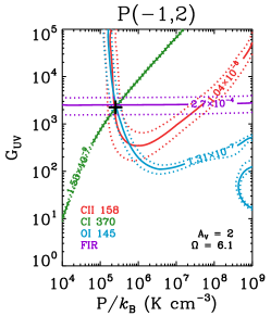
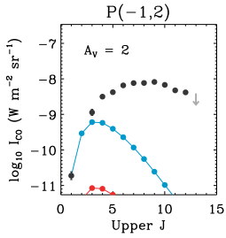
Figure 8: Meudon PDR modeling of the three fine-structure lines and the FIR luminosity. The results presented here are for the pixel $[-1,2]$, which corresponds to ($\alpha$, $\delta$)_J2000 = (05^h38^m48^s, $-69^{\circ}$04^′53^′′), and the location of this pixel is indicated as the yellow star on Fig. 9. On the left plot, the observed values and their 1$\sigma$ uncertainties are shown as the solid and dotted lines ([C ii] 158 $\mu$m, [C i] 370 $\mu$m, [O i] 145 $\mu$m, and FIR luminosity in red, green, blue, and purple). The best-fit model with the minimum $\chi^{2}$ value is presented as the black cross, and the constrained $A_{V}$ and $\Omega$ are summarized in the bottom right corner. The CO SLED predicted by the best-fit model (red; only partially shown since it is faint) is then compared with the observed CO SLED (dark and light gray for detections and non-detections) on the right plot. In addition, for an easier comparison, the predicted CO SLED is scaled up by a factor of 72 to match the observed CO(1–0) integrated intensity and shown in blue. The faint CO emission in the best-fit PDR model will be further examined in Sect. 5.1.4

.

5.1.2 Strategy for PDR modeling

The strategy for our PDR modeling was two-fold. First, we constrained $A_{V}$, $P$, and $G_{\rm UV}$ using [C ii] 158 $\mu$m, [C i] 370 $\mu$m, [O i] 145 $\mu$m, and FIR luminosity and assessed if the constrained conditions reproduce our CO observations. This is essentially what Lee et al. (2016) did for N159W, except that integrated intensities, rather than line ratios, were employed for our model fitting. As we will show in Sect. 5.1.3, however, the PDR component responsible for the fine-structure lines and FIR luminosity turned out to produce weak CO emission, and we hence further examined the conditions for CO emission by modeling CO transitions along with other observational constraints (Sect. 5.1.4). This second step was motivated by recent studies of Galactic PDRs, i.e., Joblin et al. (2018) for the Orion Bar and NGC 7023 NW and Wu et al. (2018) for the Carina Nebula, where CO SLEDs up to $J_{\rm u}$ = 23 (for the Orion Bar) were successfully reproduced by the Meudon PDR model. These studies found that high-$J$ CO emission originates from the highly pressurized ($P/k_{\rm B}\sim 10^{8}$ K cm^-3) surface of PDRs, where hot chemistry characterized by fast ion–neutral reactions take place (e.g., Goicoechea et al. 2016, 2017). Photoevaporation by strong UV radiation fields from young stars is considered to play a critical role in maintaining such high pressure at the edge of PDRs (e.g., Bron et al. 2018). In the light of these new results on the physical, chemical, and dynamical processes in PDRs, we followed the approach by Joblin et al. (2018) and Wu et al. (2018) and searched for the conditions for CO by fitting CO lines up to $J_{\rm u}$ = 13. For this, we employed the most up-to-date publicly available Meudon PDR model (version 1.5.2), as used by Joblin et al. (2018) and Wu et al. (2018).

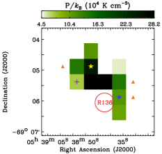
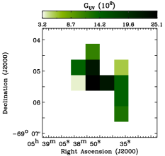
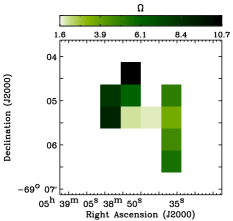
Figure 9: Best-fit PDR solutions ($P/k_{\rm B}$, $G_{\rm UV}$, and $\Omega$ on the left, middle, and right). $A_{V}$ = 2 mag was constrained for all but one pixel, and the location of this pixel with the smaller $A_{V}$ = 1.5 mag is marked with the purple cross on the left panel. The three masked pixels with unreasonably high $\Omega$ $\sim$ 30–50 are denoted as the orange triangles (Sect. 5.1.3 for details), while the pixels for Fig. 8 and Fig. 10 are indicated as the yellow and blue stars respectively. Finally, the location of R136 is shown as the red circle.

5.1.3 Modeling: fine-structure lines and FIR emission

We started PDR modeling by first examining the conditions for [C ii] 158 $\mu$m, [C i] 370 $\mu$m, [O i] 145 $\mu$m, and FIR emission. To do so, we used the PACS and SPIRE spectroscopic data on 42^′′ scales (Sect. 3), as well as the FIR luminosity map corrected for the contribution from the ionized medium ($L_{\rm FIR}^{\rm PDR}$; Appendix C for details on the correction), and derived $\chi^{2}$ for 13 pixels where all three fine-structure lines were detected (red outlined pixels in Fig. 7):

$$\chi^{2}=\sum_{i}\left[\frac{I_{i,\rm{obs}}-(\Omega I_{i,\rm{mod}})}{\sigma_{i,\rm{obs,f}}}\right]^{2},$$ (2)

where $I_{i,\rm{obs}}$ = observed integrated intensity, $\Omega I_{i,\rm{mod}}$ = model prediction scaled by the beam filling factor $\Omega$, and $\sigma_{i,\rm{obs,f}}$ = final 1$\sigma$ uncertainty in the observed integrated intensity. A large range of $\Omega$ = 10^-2–10² was considered in our $\chi^{2}$ calculation, and best-fit solutions were then identified as having minimum $\chi^{2}$ values. To demonstrate how our modeling was done, a plot of $G_{\rm UV}$ vs. $P/k_{\rm B}$ is presented in Fig. 8 for one pixel. Note that $\Omega$ $>$ 1 implies the presence of multiple components along a line of sight, e.g., Sect. 5.1 of Chevance et al. (2016) for more discussions.

For 10 out of the total 13 pixels, we found that best-fit PDR models with $P/k_{\rm B}$ = $5\times 10^{4}$$\sim$$3\times 10^{5}$ K cm^-3, $G_{\rm UV}$ = 400$\sim$2500, $\Omega$ = 2$\sim$11, and $A_{V}$ = 1.5 or 2 mag reproduce well the observed fine-structure lines and FIR luminosity. These PDR solutions are presented in Fig. 9. For the other three pixels, we then found that best-fit models have significantly higher $\Omega$ $\sim$ 30–50, as well as $P$ and $G_{\rm UV}$ that are not smooth across adjacent pixels. Our close examination, however, revealed that the observed fine-structure lines and FIR luminosity can still be reproduced within a factor of two by PDR models with $P/k_{\rm B}$ $\sim$ 10⁵ K cm^-3, $G_{\rm UV}$ $\sim$ 10³, $\Omega$ $\lesssim$ 10, and $A_{V}$ = 1.5 or 2 mag.

The images of $P$ and $G_{\rm UV}$ in Fig. 9 show that both properties peak at the north of R136 and decline outward from there. On the contrary, $\Omega$ has the minimum value of $\sim$2 at the regions where $P$ and $G_{\rm UV}$ peak and increases toward the outer edge of our coverage. While these spatial distributions of the PDR parameters are essentially consistent with what Chevance et al. (2016) found, the absolute values are quite different, e.g., the maximum $P$ and $G_{\rm UV}$ values in our analysis are a factor of $\sim$10 lower than those in Chevance et al. (2016). There are a number of factors that could contribute to the discrepancy, and our detailed comparison suggests that the difference in the angular resolution (42^′′ vs. 12^′′) is most likely the primary factor (Appendix D). The same resolution effect was also noted by Chevance et al. (2016), stressing the importance of high spatial resolution in the studies of stellar radiative feedback. Finally, we note that the existence of several clouds whose individual $A_{V}$ is roughly 2 mag is indeed in agreement with what we estimated from dust SED modeling ($A_{V}$ $\sim$ 8–20 mag; Sect. 3.5), implying that the PDR component for the fine-structure lines and FIR luminosity constitutes a significant fraction ($\gtrsim$ 50%) of dust extinction along the observed lines of sight.

Interestingly, we found that CO emission is quite faint in the constrained PDR conditions. To be specific, the PDR models underestimate the observed CO integrated intensities by at least a factor of 10, and the discrepancy becomes greater with increasing $J$, e.g., from a factor of $\sim$10–70 for CO(1–0) to a factor of $\sim$(2–5) $\times$ 10⁵ for CO(13–12). The worsening discrepancy with increasing $J$ suggests that the shape of the observed CO SLEDs is not reproduced by the PDR models, and we indeed found that the predicted CO SLEDs peak at $J$=3–2, which is much lower than the observed $J_{\rm p}$ $\geq$ 6–5. This large discrepancy between our CO observations and the model predictions (in terms of both the amplitude and shape of the CO SLEDs) is clearly demonstrated in Fig. 8. Finally, we note that the H₂ 0–0 S(3) line is predicted to be as bright as $\sim$2 $\times$ (10^-9–10^-8) W m^-2 sr^-1, which is consistent with the measured upper limits based on 5$\sigma_{\rm s}$ (unfortunately, H₂ 0–0 S(3) is not detected over the 13 pixels where PDR modeling was performed).

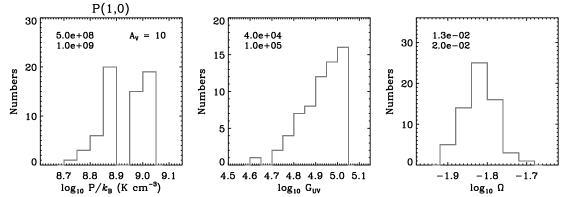
Figure 10: PDR models with $A_{V}$ = 10 mag that were selected by the criteria in Sect. 5.1.4 ($P/k_{\rm B}$, $G_{\rm UV}$, and $\Omega$ on the left, middle, and right panels; number of selected models = 64). This particular example is for the pixel $[1,0]$ (corresponding to ($\alpha$, $\delta$)_J2000 = (05^h38^m37^s, $-69^{\circ}$05^′53^′′)), and the location of the pixel is indicated as the blue star in Fig. 9. In each plot, the minimum and maximum values of the PDR parameter are shown in the top left corner.

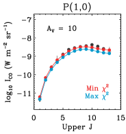
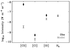
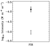
Figure 11: Comparison between the observations and the predictions from the PDR models in Fig. 10. In the left plot, the observed CO SLED (dark and light gray for detections and non-detections) is compared with the predictions from two models (those resulting in minimum and maximum $\chi^{2}$ values with respect to the observed CO lines are presented in red and blue). In the middle and right plots, the observed [C ii] 158 $\mu$m, [C i] 370 $\mu$m, [O i] 145 $\mu$m, H₂ 0–0 S(3), and FIR luminosity are shown (black) along with the ranges of the model predictions (from minimum to maximum values; gray).

5.1.4 Modeling: CO lines

Our modeling in Sect. 5.1.3 strongly suggests that CO emission in 30 Doradus arises from the conditions that are drastically different from those for the fine-structure lines and FIR luminosity, i.e., $P/k_{\rm B}$ = a few (10⁴–10⁵) K cm^-3, $G_{\rm UV}$ = a few (10²–10³), and $A_{V}$ $\sim$ 2 mag. More precisely, the CO-emitting regions would most likely have higher densities and/or higher temperatures (to have $J_{\rm p}$ $\geq$ 6–5), as well as higher dust extinction (to form more CO molecules, leading to brighter emission), than the [C ii] 158 $\mu$m-emitting regions. This conclusion is essentially the same as what Lee et al. (2016) found for N159W. We then went one step further by modeling the observed CO transitions, examining the PDR conditions from which the CO-emitting gas would arise.

Initially, we began by computing $\chi^{2}$ using CO transitions up to $J$=13–12 and finding best-fit PDR models with minimum $\chi^{2}$ values. This exercise, however, revealed that the models become highly degenerate once high $A_{V}$ ($\gtrsim$ 5 mag), $P/k_{\rm B}$ ($\gtrsim$ 10⁸ K cm^-3), and $G_{\rm UV}$ ($\gtrsim$ 10³) are achieved. In addition, many best-fit models were incompatible with the observed fine-structure lines and FIR luminosity. Specifically, the best-fit models always underestimate [C ii] 158 $\mu$m and FIR luminosity (model-to-observation ratio $\lesssim$ 0.1), while mostly reproducing [O i] 145 $\mu$m and [C i] 370 $\mu$m within a factor of four or less. As for H₂ 0–0 S(3), the best-fit models predict too bright emission in many cases. This result hints that at least two components, the low-$P$ and high-$P$ PDRs, would be required to explain all the transitions we observed in 30 Doradus. To work around the degeneracy issue and exclude models with unreasonable predictions for the fine-structure lines and FIR luminosity, we then decided to evaluate a collection of PDR models that reproduce the observed CO reasonably well, rather than focusing on best-fit models, and employ other observations as secondary constraints. To this end, we selected the PDR models that satisfy the following criteria: (1) The detected CO lines are reproduced within a factor of two. In the case of CO(1–0), the prediction is only required not to exceed twice the observed value, considering that CO(1–0) could trace different physical conditions than intermediate- and high-$J$ CO lines (e.g., Joblin et al. 2018; Wu et al. 2018). (2) The model predictions agree with the measured upper limits when the CO lines are not detected. (3) For [C ii] 158 $\mu$m, [C i] 370 $\mu$m, [O i] 145 $\mu$m, and FIR luminosity, the model predictions plus the contributions from the low-$P$ PDR component in Sect. 5.1.3 are within a factor of two from the observed values. (4) Finally, the model prediction plus the contribution from the low-$P$ PDR component should be consistent with the H₂ 0–0 S(3) upper limit. These four criteria were applied to the 10 pixels where we constrained the best-fit PDR models for the fine-structure lines and FIR luminosity (Fig. 9), along with a large range of $\Omega$ = 10^-4–1 in consideration. Since bright CO($J$ $\gtrsim$ 4–3) emission mostly arises from a relatively narrow range of physical conditions ($A_{V}$ $\gtrsim$ 5 mag, $P/k_{\rm B}$ $\gtrsim$ 10⁸ K cm^-3, and $G_{\rm UV}$ $\gtrsim$ 10³) in the Meudon PDR model, slight changes in modeling, e.g., removing the (3) and (4) criteria or modeling CO lines with $J$ $\gtrsim$ 4–3 only, do not make a large impact on the constrained parameters. Finally, we note that our modeling with two components of gas is simplistic, given that multiple components would likely be mixed on $\sim$10 pc scales. Nevertheless, our analyses would still provide average physical conditions of the components within the beam.

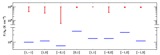
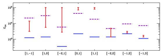
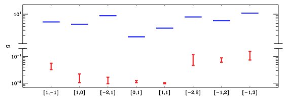
Figure 12: Comparison between the low- and high-$P$ PDR models ($P/k_{\rm B}$, $G_{\rm UV}$, and $\Omega$ on the top, middle, and bottom panels). In each plot, the low-$P$ models we constrained using the fine-structure lines and FIR luminosity (Sect. 5.1.3) are indicated as the blue solid lines, while the high-$P$ models for the CO lines are presented as the red bars (ranging from the minimum to maximum values). In the $G_{\rm UV}$ plot, $G_{\rm stars}$ in Fig. 7 is also shown as the purple dashed lines. In total, eight pixels where we found reasonably good high-$P$ models are shown in each plot, and the location of each pixel can be inferred from, e.g., Fig. 3 and Fig. 5. Finally, note that the $P$ and $\Omega$ plots have broken $y$-axes to show a wide range of the data.

Overall, we were able to find reasonably good PDR solutions that meet the above selection criteria for eight out of the total 10 pixels ($[-1,1]$ and $[1,2]$ do not have solutions). The constrained parameters were then as follows: $A_{V}$ = 5–40 mag, $P/k_{\rm B}$ = $\sim$10⁸–10⁹ K cm^-3, $G_{\rm UV}$ = $\sim$10³–10⁵, and $\Omega$ = $\sim$0.01–0.1. Note that $A_{V}$ was not well constrained, since increasing $A_{V}$ beyond 5 mag only increases the size of the cold CO core ($<$ 50 K) in a PDR, not the warm layer ($\gtrsim$ 50–100 K) where most of intermediate- and high-$J$ CO emission originates (e.g., Sect. 6.1). In addition, $\Omega$ $\sim$ 0.01–0.1 implies that the CO-emitting clumps would be $\sim$0.7–2 pc in size, which is consistent with the ALMA CO(2–1) observations where CO emission was found to primarily arise from $\sim$0.3–1 pc size structures (Indebetouw et al. 2013). In Fig. 10 and Fig. 11, we then present the selected PDR models for one pixel, as well as the predicted line and continuum intensities, as an example.

Interestingly, we found that the constrained PDR models significantly underestimate [C ii] 158 $\mu$m and FIR luminosity (e.g., Fig. 11): the discrepancy with our data ranges from $\sim$100 to $\sim$10³ for [C ii] 158 $\mu$m and from $\sim$10 to $\sim$100 for FIR luminosity. On the other hand, [O i] 145 $\mu$m and [C i] 370 $\mu$m were marginally reproduced (within a factor of four or less) in most cases: four out of the eight pixels for [O i] 145 $\mu$m and seven out of the eight pixels for [C i] 370 $\mu$m. The measured H₂ 0–0 S(3) upper limits were also consistent with the model predictions. All in all, these results indicate that at least two PDR components are needed to explain all the observational constraints we have for 30 Doradus: (1) the low-$P$ (10⁴–10⁵ K cm^-3) component that provides most of the dust extinction along the observed lines of sight and emits intensely in [C ii] 158 $\mu$m and FIR continuum and (2) the high-$P$ (10⁸–10⁹ K cm^-3) component that is mainly responsible for CO emission. For [O i] 145 $\mu$m, [C i] 370 $\mu$m, and H₂ 0–0 S(3), both components contribute. We indeed confirmed that the sum of the two components fully reproduces the observations in our study (including CO $J$=1–0).

To understand how different the two components are in terms of their physical properties, we then made a comparison between the constrained PDR parameters on a pixel-by-pixel basis (Fig. 12). Our comparison revealed first of all that the high-$P$ component indeed has significantly higher $P$ than the low-$P$ component (a factor of $\sim$10³–10⁴). Combined with the fact that the high-$P$ models have much smaller $\Omega$ than the low-$P$ models (a factor of $\sim$10²–10³), this result implies that the CO-emitting regions in 30 Doradus are more compact, as well as warmer and/or denser, than the [C ii]-emitting regions. The relative distribution of the two regions can then be inferred from the $G_{\rm UV}$ values. For most of the pixels in our consideration, we found that the UV radiation incident onto the surface of the CO-emitting regions is more intense than that for the [C ii]-emitting regions (by up to a factor of $\sim$300). These pixels also have $G_{\rm stars}$ that is comparable to or slightly higher than $G_{\rm UV}$ for the high-$P$ component. Considering that the UV radiation field would be most intense on the plane of R136 ($G_{\rm stars}$) and decrease as the distance $r$ from R136 increases ($\propto$ 1/$r^{2}$ if no absorption is taken into account), our results imply that the CO-emitting regions would likely be either in between R136 and the [C ii]-emitting regions or much closer to R136. For the pixel $[1,1]$ though, $G_{\rm UV}$ for the high-$P$ component is higher than $G_{\rm stars}$ by up to a factor of $\sim$5, a somewhat large discrepancy even considering uncertainties in $G_{\rm UV}$ and $G_{\rm stars}$ (so the PDR solution could be unreasonable).

In summary, we conclude that the observed CO transitions in 30 Doradus (up to $J$=13–12) could be powered by UV photons and likely originate from highly compressed ($P/k_{\rm B}$ $\sim$ 10⁸–10⁹ K cm^-3), highly illuminated ($G_{\rm UV}$ $\sim$ 10³–10⁵) clumps with a scale of $\sim$0.7–2 pc. These clumps are also partially responsible for the observed [C i] 370 $\mu$m and [O i] 145 $\mu$m, but emit quite faintly in [C ii] 158 $\mu$m and FIR continuum emission, hinting the presence of another component with drastically different physical properties. Our PDR modeling then suggests that this additional component indeed has lower $P$ (a few (10⁴–10⁵) K cm^-3) and $G_{\rm UV}$ (a few (10²–10³)) and likely fills a large fraction of our 30^′′-size pixels. Interestingly, the constrained PDR parameters imply that the two distinct components are likely not co-spatial (the high-$P$ PDR component closer to R136), which is a somewhat unusual geometry. More detailed properties of the two components, e.g., gas density and temperature, will be discussed in Sect. 6.1, along with another viable heating source for CO, shocks.

Figure 13: Degeneracy in $n_{\rm pre}$ and $\varv_{\rm s}$. To illustrate this issue, the observed CO and H₂ 0–0 S(3) transitions of the pixel $[-1,2]$ are shown in the left and right plots along with three different shock models ($``$M1$"$ in red: $n_{\rm pre}$ = 10<sup>4</sup> cm<sup>-3</sup> and $\varv_{\rm s}$ = 28 km s<sup>-1</sup>; $``$M2$"$ in green: $n_{\rm pre}$ = 5 $\times$ 10⁴ cm^-3 and $\varv_{\rm s}$ = 7.5 km s^-1; $``$M3$"$ in blue: $n_{\rm pre}$ = 10⁶ cm^-3 and $\varv_{\rm s}$ = 4 km s^-1). For both plots, dark and light gray colors are used to represent detections and non-detections, and $G^{\prime}_{\rm UV}$ = 0 and $\Omega$ $\sim$ 0.1 are adopted for the three shock models.

5.2 Radiative source: X-rays and cosmic-rays

As described in Sect. 2.3, abundant X-rays and cosmic-rays exist in 30 Doradus. These high energy photons and particles can play an important role in gas heating (mainly through photoionization of atoms and molecules), and yet we evaluated that their impact on the observed CO lines is negligible. Our evaluation was based on Lee et al. (2016) and can be summarized as follows.

In Lee et al. (2016), we examined the influence of X-rays by considering the most luminous X-ray source in the LMC, LMC X-1 (a black hole binary). The maximum incident X-ray flux of 10^-2 erg s^-1 cm^-2 (maximum since absorption between LMC X-1 and N159W was not taken into account) was incorporated into PDR modeling, and we found that X-rays make only a factor of three or so change in the total CO integrated intensity. Considering that the X-ray flux in 30 Doradus is much lower (up to 10^-4 erg s^-1 cm^-2 only) than the maximum case for N159W, we then concluded that X-rays most likely provide only a minor contribution to CO heating in 30 Doradus.

As for cosmic-ray heating, we again followed the simple calculation by Lee et al. (2016). In this calculation, H₂ cooling (primary cooling process for the warm and dense medium; e.g., Le Bourlot et al. 1999) was equated with cosmic-ray heating to estimate the cosmic-ray ionization rate of $\zeta_{\rm CR}$ $\gtrsim$ 3 $\times$ 10^-13 s^-1 that is required to fully explain the warm CO in N159W. While this cosmic-ray ionization rate is higher than the typical value for the diffuse ISM in the solar neighborhood by more than a factor of 1000 (e.g., Indriolo et al. 2015), the measured $\gamma$-ray emissivity of N159W ($\sim$10²⁶ photons s^-1 sr^-1 per hydrogen atom) is comparable to the local ISM value (e.g., Abdo et al. 2009), suggesting that the cosmic-ray density in N159W is not atypical. Similarly, considering that the CO-emitting gas in 30 Doradus is warm and dense as in N159W (Sect. 6.1 for details), yet the $\gamma$-ray emissivity is only $\sim$3 $\times$ 10²⁶ photons s^-1 sr^-1 per hydrogen atom (Abdo et al. 2010), it is again likely that cosmic-rays in 30 Doradus are not abundant enough for CO heating.

5.3 Mechanical source: shocks

Shocks are ubiquitous in the ISM, being continuously driven by various energetic processes, e.g., stellar activities such as outflows (YSOs and red giant stars), winds (OB and W-R stars), and explosions (novae and supernovae), as well as non-stellar activities such as colliding clouds and spiral density waves (e.g., Hollenbach et al. 1989). These shocks can be an important source of heating, since they effectively transform the bulk of the injected mechanical energy into thermal energy. In the particular case of the dense and magnetized medium with a low fractional ionization (essentially corresponding to star-forming regions such as 30 Doradus), C-type shocks can develop, whose main characteristics include: (1) molecules are accelerated without being thermally dissociated; and (2) the shocked medium radiates primarily in rotation-vibration transitions of molecules, as well as fine-structure lines of atoms and ions (Draine & McKee 1993). The emission from C-type shocks largely appears at IR wavelengths and provides a powerful means to probe the physical properties of the shocks and the ambient medium.

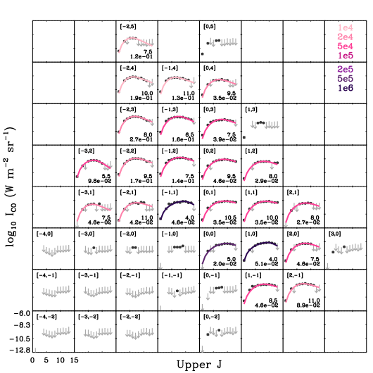
Figure 14: Constrained shock models overlaid with the observed CO SLEDs. As in Fig. 5, the circles and downward arrows represent the measured intensities and 5$\sigma_{\rm s}$-based upper limits. A location with respect to the pixel that is closest to R136 is also indicated as a pair of numbers in the top left corner of each pixel (e.g., [0,0] corresponds to ($\alpha$, $\delta$)_J2000 = (05^h38^m42^s, $-69^{\circ}$05^′53^′′), and each pixel is in 30^′′ size). The shock models with different $n_{\rm pre}$ are presented in different colors (darker shades for higher $n_{\rm pre}$), and the exact $n_{\rm pre}$ values (in cm^-3) are summarized in the top right corner of this figure. Finally, the constrained shock velocities (in km s^-1) and beam filling factors (unitless) are shown in the bottom right corner of each pixel.

5.3.1 Paris-Durham shock model

Motivated by the results from Lee et al. (2016) for N159W, we evaluated whether low-velocity C-type shocks could be another important source of heating for CO in 30 Doradus by comparing the observed line emission with predictions from the Paris-Durham shock model⁷ (Flower & Pineau des Forêts 2015). This one-dimensional stationary model simulates the propagation of a shock wave (J- or C-type) through a layer of gas and dust and calculates the physical, chemical, and dynamical properties of the shocked layer. For our analysis, we used the modified version by Lesaffre et al. (2013) to model UV-irradiated shocks and created a grid of models with the following parameters: (1) pre-shock density $n_{\rm pre}$ = (1, 2, and 5) $\times$ 10⁴, (1, 2, and 5) $\times$ 10⁵, and 10⁶ cm^-3, (2) shock velocity $\varv_{\rm s}$ = 4–11 km s^-1 with 0.5 km s^-1 steps and 12–30 km s^-1 with 2 km s^-1 steps (a finer grid was produced for $\varv_{\rm s}$ = 4–11 km s^-1 to properly sample a factor of $\sim$100 variation in H₂ 0–0 S(3) over this velocity range), (3) UV radiation field $G^{\prime}_{\rm UV}$ (defined as a scaling factor relative to the Draine 1978 radiation field) = 0 and 1, (4) dimensionless magnetic field parameter $b$ = 1 (defined as ($B$/$\mu$G)/($n_{\rm pre}$/cm^-3)^1/2, where $B$ is the strength of the magnetic field transverse to the direction of shock propagation), and (5) same gas and dust properties as used in our PDR modeling (Table 2 for details). In our grid of models, the magnetosonic speed varies from $\sim$20 km s^-1 ($G^{\prime}_{\rm UV}$ = 1 case) to $\sim$80 km s^-1 ($G^{\prime}_{\rm UV}$ = 0 case), and the post-shock pressure (roughly determined by the ram-pressure of the pre-shock medium) has a range of $\sim$10⁵–10⁹ K cm^-3. All our models fall into the C-type shock category. Finally, the calculated abundances of atoms and molecules were post-processed via the LVG method by Gusdorf et al. (2012, 2015) to compute level populations, line emissivities, and integrated intensities.

5.3.2 Strategy for shock modeling

To examine the properties of shocks that could possibly heat CO in 30 Doradus, we went one step further than Lee et al. (2016) by fitting the observed CO transitions with the shock models. In an attempt to break the degeneracy between the model parameters, we then considered other constraints as well, such as H₂ 0–0 S(3) and [C i] 370 $\mu$m, in our shock modeling.

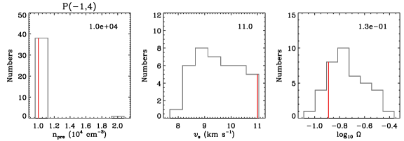
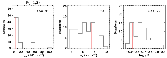
Figure 15: Another illustration of the degeneracy in our shock modeling. Here the selected “good” shock models that reproduce our CO and H₂ 0–0 S(3) observations within a factor of two are presented for two pixels, $[-1,4]$ and $[-1,2]$ (top and bottom; number of the selected models = 39 and 67 respectively), as the gray histograms. For each histogram, the final shock parameter we constrained in Sect. 5.3.3 is shown as the red solid line and summarized on the top right corner. A comparison between the top and bottom histograms clearly shows that $[-1,4]$ has a quite narrow distribution of $n_{\rm pre}$.

5.3.3 Modeling: CO lines

We began shock modeling by first deriving $\chi^{2}$ using the observed CO ($J$=3–2 to 13–12) and H₂ 0–0 S(3) transitions for 23 pixels that contain more than five CO detections (so that the number of constraints $\geq$ 1 + the number of model parameters, $n_{\rm pre}$, $\varv_{\rm s}$, $G^{\prime}_{\rm UV}$, and $\Omega$). Our $\chi^{2}$ calculation was essentially based on Eq. (2), but with an additional consideration for non-detections. Specifically, we set $[I_{i,\rm{obs}}-(\Omega I_{i,\rm{mod}})]$/$\sigma_{i,\rm{obs,f}}$ = 0 for the transitions whose 5$\sigma_{\rm s}$-based upper limits are consistent with model predictions. When the model predictions are higher than the upper limits, we then simply excluded such bad models from our analysis (so the non-detections were used only to provide hard limits on the models). In our $\chi^{2}$ analysis, CO(1–0) was not included to consider a possible presence of some cold pre-shock gas that could emit brightly in CO(1–0) (e.g., Lee et al. 2016). Finally, the same $\Omega$ = 10^-4–1 as used in our PDR modeling (Sect. 5.1.4) was examined.

The inclusion of H₂ 0–0 S(3) in our $\chi^{2}$ analysis was intended to mitigate the degeneracy between $n_{\rm pre}$ and $\varv_{\rm s}$. In particular, we found that H₂ 0–0 S(3), even with upper limits, can effectively differentiate high-density ($>$ 10⁴ cm^-3), low-velocity ($\lesssim$ 10 km s^-1) shocks from low-density ($\sim$10⁴ cm^-3), high-velocity ($\gtrsim$ 20 km s^-1) shocks. To demonstrate this, we show the observed CO and H₂ 0–0 S(3) for the pixel $[-1,2]$ in Fig. 13, along with three different shock models ($n_{\rm pre}$ = 10⁴, 5 $\times$ 10⁴, and 10⁶ cm^-3; $\varv_{\rm s}$ = 28, 7.5, and 4 km s^-1; $G^{\prime}_{\rm UV}$ = 0; $\Omega$ $\sim$ 0.1). These shock models all reproduce the observed CO SLED within a factor of two, while showing a factor of $\sim$200 difference in H₂ 0–0 S(3). Specifically, the highest-velocity shock produces the brightest H₂ 0–0 S(3) of $\sim$4 $\times$ 10^-7 W m^-2 sr^-1 (primarily due to the high temperature of $\sim$10³ K that is achieved by strong compression), and the measured upper limit clearly rules out this model. On the other hand, the other two models have relatively low temperatures of $\sim$10² K and show an insignificant difference in H₂ 0–0 S(3) emission (a factor of four). Our H₂ observations, unfortunately, are not sensitive enough to discriminate this level of minor difference (e.g., only two out of the total 23 pixels have detections with $S/N_{\rm s}$ $\sim$ 5), resulting in the degeneracy in 5 $\times$ 10⁴ cm^-3 $\lesssim$ $n_{\rm pre}$ $\lesssim$ 10⁶ cm^-3 and $\varv_{\rm s}$ $\lesssim$ 10 km s^-1 in our shock analysis.

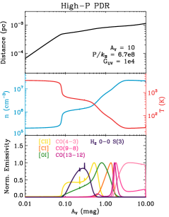
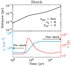
Figure 16: Physical properties of the PDR and shock components in 30 Doradus. The following three models are presented as examples: (1) low-$P$ PDR with $A_{V}$ = 2 mag, $P/k_{\rm B}$ = 10⁵ K cm^-3, and $G_{\rm UV}$ = 10³ (left), (2) high-$P$ PDR with $A_{V}$ = 10 mag, $P/k_{\rm B}$ = 6.7 $\times$ 10⁸ K cm^-3, and $G_{\rm UV}$ = 10⁴ (middle), and (3) shock with $n_{\rm pre}$ = 5 $\times$ 10⁴ cm^-3, $\varv_{\rm s}$ = 8 km s^-1, and $G^{\prime}_{\rm UV}$ = 0 (right). For the two PDR models, several physical quantities (top: distance; middle: density and temperature; bottom: normalized emissivities of [C ii] 158 $\mu$m, [C i] 370 $\mu$m, and [O i] 145 $\mu$m, as well as selected CO and H₂ transitions) are shown as a function of dust extinction. For the shock model, the distance (measured along the direction of propagation of the shock wave; top), as well as the density and temperature of the neutral fluid (bottom), are plotted as a function of flow time.

In addition to $n_{\rm pre}$ and $\varv_{\rm s}$, $G^{\prime}_{\rm UV}$ and $\Omega$ are degenerate as well in the shock models ($G^{\prime}_{\rm UV}$ = 1 would dissociate more CO molecules than the $G^{\prime}_{\rm UV}$ = 0 case, requiring a larger beam filling factor to achieve the same level of CO emission), and we tried to mitigate this degeneracy by considering the observed [C i] 370 $\mu$m emission. For example, eight out of the total 23 pixels in our shock analysis have best-fit models with $G^{\prime}_{\rm UV}$ = 1, and these $G^{\prime}_{\rm UV}$ = 1 models overpredict [C i] 370 $\mu$m by a factor of $\sim$10–20. In addition, the constrained $\Omega$ for these models is close to one, which is not compatible with what the high resolution ALMA CO(2–1) observations suggest ($\Omega$ $\lesssim$ 0.1). Considering that this is indeed a general trend (shock models with $G^{\prime}_{\rm UV}$ = 1 that reproduce our CO and H₂ 0–0 S(3) observations tend to overpredict [C i] 370 $\mu$m with unreasonably larger beam filling factors of $\sim$1), we then determined final shock properties by selecting $G^{\prime}_{\rm UV}$ = 0 models with minimum $\chi^{2}$ values and present them in Fig. 14.

Overall, we found that single shock models with $n_{\rm pre}$ $\sim$ 10⁴–10⁶ cm^-3, $\varv_{\rm s}$ $\sim$ 5–10 km s^-1, $\Omega$ $\sim$ 0.01–0.1, and no UV radiation field reproduce our CO and H₂ 0–0 S(3) observations reasonably well. The constrained $\varv_{\rm s}$ and $\Omega$ values seem to be consistent with previous studies as well ($\varv_{\rm s}$: the 30^′′-scale CO(7–6) spectrum obtained by Pineda et al. (2012) shows a linewdith of $\sim$10 km s^-1; $\Omega$: the ALMA CO(2–1) observations by Indebetouw et al. (2013) suggest $\Omega$ $\lesssim$ 0.1), implying that our final shock models are reasonable. Considering the degeneracy that persists in our modeling, we will not discuss the shock parameters on a pixel-by-pixel basis (our solutions in Fig. 14 should be considered as approximative models) and instead focus on large-scale trends. For example, we examined the parameter space of “good” shock models that reproduce our CO and H₂ 0–0 S(3) observations within a factor of two and found that top pixels, e.g., $[-2,5]$, $[-2,4]$, and $[-1,4]$, indeed likely have a lower density of $\sim$10⁴ cm^-2 compared to other pixels, based on a narrow distribution of $n_{\rm pre}$ (Fig. 15).

While reproducing the observed CO (including $J$=1–0; the shocked medium produces $\sim$30–80% of the observed emission) and H₂ 0–0 S(3) transitions reasonably well, the shock models predict quite faint fine-structure lines. Specifically, we found that the model-to-observed line ratios are only $\lesssim$ 4 $\times$ 10^-6, $\lesssim$ 0.01, $\lesssim$ 0.03 for [C ii] 158 $\mu$m, [C i] 370 $\mu$m, and [O i] 145 $\mu$m. This result implies that at least two ISM components are required to fully explain our observations of 30 Doradus, and the likely possibility in the shock scenario for CO would then be: (1) the low-$P$ PDR component (10⁴–10⁵ K cm^-3; Sect. 5.1.3) that primarily contributes to the observed [C ii] 158 $\mu$m, [C i] 370 $\mu$m, [O i] 145 $\mu$m, and FIR emission and (2) the high-$P$ shock component (10⁷–10⁸ K cm^-3; Sect. 6.1 for details) that radiates intensely mainly in CO. In the case of H₂ 0–0 S(3), both components contribute, and the combined contributions are still consistent with the measured upper limits. The shock-to-PDR ratio significantly varies from $\sim$0.1 to $\sim$6 for H₂ 0–0 S(3), which could be partly due to the degeneracy we still have in $n_{\rm pre}$ and $\varv_{\rm s}$.

In short, we conclude that low-velocity C-type shocks with $n_{\rm pre}$ $\sim$ 10⁴–10⁶ cm^-3 and $\varv_{\rm s}$ $\sim$ 5–10 km s^-1 could be another important source of excitation for CO in 30 Doradus. The shock-compressed ($P/k_{\rm B}$ $\sim$ 10⁷–10⁸ K cm^-3) CO-emitting clumps are likely $\sim$0.7–2 pc in size and embedded within some low-$P$ ($P/k_{\rm B}$ $\sim$ 10⁴–10⁵ K cm^-3), UV-irradiated ($G_{\rm UV}$ $\sim$ 10²–10³) ISM component that produces bright [C ii] 158 $\mu$m, [C i] 370 $\mu$m, [O i] 145 $\mu$m, and FIR continuum emission. This low-$P$ PDR component fills a large fraction of our 30^′′-size pixels and provides up to $A_{V}$ $\sim$ 4–20 mag, shielding the shocked CO clumps from the dissociating UV radiation field. In the next sections, we will then present more detailed physical properties (e.g., density, temperature, etc.) of these shock and low-$P$ PDR components and compare them to those of the high-$P$ PDR component (Sect. 5.1.4), with an aim of probing the origin of CO emission in 30 Doradus.

6 Discussions

6.1 Physical conditions of the neutral gas

6.1.1 Low thermal pressure component

We start our discussion by first presenting several physical quantities ($n$, $T$, and line emissivities) of a representative low-$P$ PDR model ($A_{V}$ = 2 mag, $P/k_{\rm B}$ = 10⁵ K cm^-3, and $G_{\rm UV}$ = 10³) as a function of $A_{V}$ in Fig. 16. As described throughout Sect. 5, this low-$P$ PDR component is primarily bright in [C ii] 158 $\mu$m, [C i] 370 $\mu$m, [O i] 145 $\mu$m, and FIR continuum emission and essential to fully reproduce our multi-wavelength data of 30 Doradus.

A close examination of the radial profiles in Fig. 16 suggests that CO emission mostly originates from a diffuse and relatively warm medium with $n$ $\sim$ a few 100 cm^-3 and $T$ $\lesssim$ 100 K. The CO abundance in this diffuse and extended (line-of-sight depth of $\sim$6 pc) PDR component is low ($N$(CO) $\sim$ a few 10¹³ cm^-2), which likely results from the following two aspects: (1) The slab of gas with relatively low dust extinction is illuminated by a strong UV radiation field. (2) The density is low. This low CO abundance is likely the primary reason for why the low-$P$ PDR component is so faint in CO emission.

6.1.2 High thermal pressure component

Our analysis above indicates that high densities and/or temperatures would be needed for the observed bright CO emission, and we found that it is indeed the case for the high-$P$ PDR and shock components. For an illustration, we then again select representative high-$P$ PDR ($A_{V}$ = 10 mag, $P/k_{\rm B}$ = 6.7 $\times$ 10⁸ K cm^-3, and $G_{\rm UV}$ = 10⁴) and shock ($n_{\rm pre}$ = 5 $\times$ 10⁴ cm^-3, $\varv_{\rm s}$ = 8 km s^-1, and $G^{\prime}_{\rm UV}$ = 0) models and present their profiles in Fig. 16. Note that the shock profiles are different from those for the PDR models, in a way that they are shown as a function of the flow time through the shock structure (from the pre- to post-shock medium), rather than dust extinction.

The profiles in Fig. 16 clearly show that the high-$P$ PDR has quite different conditions for CO emission compared to the low-$P$ PDR. For example, we found that low-$J$ CO lines are emitted from a highly dense and cold medium with $n$ $\gtrsim$ 10⁷ cm^-3 and $T$ $\sim$ 30 K, while intermediate- and high-$J$ CO lines mainly arise from a relatively warm layer with $n$ $\sim$ a few 10⁶ cm^-3 and $T$ $\sim$ 100 K. The bright CO emission from this dense and highly compressed PDR component (line-of-sight depth of $\sim$10^-3 pc) is likely due to abundant CO molecules ($N$(CO) $\sim$ a few 10¹⁸ cm^-2), which result from the sufficient dust extinction ($A_{V}$ $\gtrsim$ 5 mag) to protect CO from photodissociation, as well as from the high density.

The physical properties of the high-$P$ PDR component seem slightly different from those of the low-velocity C-type shocks as well. Specifically, for the constrained shock models in Fig. 14, we found that the shock-compressed CO-emitting layer (line-of-sight depth of $\sim$10^-2 pc) is less dense ($n$ $\sim$ a few (10⁴–10⁶) cm^-3) and less CO abundant ($N$(CO) $\sim$ a few (10¹⁶–10¹⁷) cm^-2), while having a higher temperature ($T$ $\sim$ 100–500 K), than the high-$P$ PDR counterpart.

6.2 Source of the high thermal pressure

Our analyses suggest that the observed CO emission in 30 Doradus most likely originates from strongly compressed regions, whose high pressure ($P/k_{\rm B}$ $\sim$ 10⁷–10⁹ K cm^-3) could be driven by either UV photons or shocks. Here we examine the likelihood of each case based on the known characteristics of 30 Doradus.

6.2.1 UV photons

If UV photons are the dominant source of the high thermal pressure in the CO-emitting regions, we would expect somehow a correlation between stellar properties (e.g., spectral type, stellar density, etc.) and the constrained PDR conditions. Such a correlation was indeed predicted recently by the photoevaporating PDR model of Bron et al. (2018), where one-dimensional hydrodynamics, UV radiative transfer, and time-dependent thermo-chemical evolution are calculated simultaneously for a molecular cloud exposed to an adjacent massive star. In this model, the UV-illuminated surface of the cloud can freely evaporate into the surrounding gas, and this photoevaporation at the ionization and dissociation fronts produces high pressure (up to $\sim$10⁹ K cm^-3). One of the predicted aspects of the photoevaporating PDR was a linear relation between $P/k_{\rm B}$ and $G_{\rm UV}$, whose slope depends on the spectral type of the star, e.g., the $P/k_{\rm B}$-to-$G_{\rm UV}$ ratios of $\sim$5 $\times$ 10³ and $\sim$8 $\times$ 10⁴ for B- and O-type stars (higher ratios for hotter stars). This prediction seems to reproduce the observations of several Galactic PDRs (e.g., Joblin et al. 2018; Wu et al. 2018) and is shown in Fig. 17.

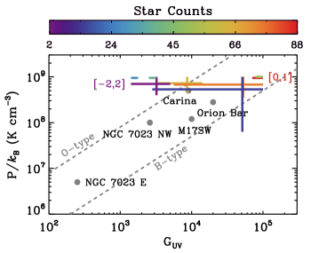
Figure 17: $P/k_{\rm B}$ as a function of $G_{\rm UV}$ for various Galactic and extragalactic sources. The high-$P$ PDR conditions for CO emission in 30 Doradus are presented as the bars (same as in Fig 12) in different colors depending on star counts, while other sources are shown as the gray circles (Orion Bar and NGC 7023 NW from Joblin et al. 2018; Carina Nebula from Wu et al. 2018; NGC 7023 E from Köhler et al. 2014; M17SW from Pérez-Beaupuits et al. 2010). In addition, the two pixels we discuss in the main text, [$-$2,2] and [0,1], are indicated, along with the predictions from Bron et al. (2018) for B- and O-type stars (gray dashed lines; $P/k_{\rm B}$-to-$G_{\rm UV}$ ratio = 5 $\times$ 10³ and 8 $\times$ 10⁴ respectively).

To evaluate whether UV photons are indeed responsible for the high thermal pressure in the CO-emitting regions, we examined the constrained high-$P$ PDR solutions in combination with the observed stellar properties. As an illustration, the minimum and maximum values of $P/k_{\rm B}$ and $G_{\rm UV}$ are indicated in Fig. 17 as bars in different colors depending on star counts. Here the star counts were estimated by counting the number of stars that fall into each FTS pixel in 30^′′ size ($\sim$1.3 $\times$ 10⁴ stars we used for the derivation of $G_{\rm stars}$ were considered; Fig. 7 and Appendix B) and were found to vary by a factor of $\sim$40 from 2 to 88 for the eight pixels in our consideration. The measured $P/k_{\rm B}$ and $G_{\rm UV}$ values of 30 Doradus appear to be in reasonably good agreement with the predictions from Bron et al. (2018), but a close examination revealed that some of the observed trends are actually against expectations for UV-driven high pressure. For example, the pixels [$-$2,2] and [0,1] have the minimum and maximum star count respectively, yet their thermal pressures are comparable ($\sim$(0.5–1) $\times$ 10⁹ K cm^-3). Considering that the high-$P$ PDR components of both pixels are equally likely quite close to the plane of R136 (inferred from similar $G_{\rm UV}$ and $G_{\rm stars}$ values; Fig. 12), it is indeed difficult to reconcile the comparable thermal pressures with a factor of $\sim$40 different star counts. In addition, [0,1] has a factor of $\sim$20 lower $P/k_{\rm B}$-to-$G_{\rm UV}$ ratio than [$-$2,2], even though it has more hotter stars, i.e., 13 stars with $T_{\rm eff}$ $\geq$ 4 $\times$ 10⁴ K exist for [0,1], while none for [$-$2,2]. This result is in contrast with what Bron et al. (2018) predicts.

In summary, we conclude that while the Meudon PDR model reproduces the observed CO lines, the constrained PDR conditions are not in line with what we would expect based on the stellar content of 30 Doradus. This conclusion, however, is tentative and needs further examinations, since our current analyses have several limitations. For example, we analyzed the CO and fine-structure line observations of 30 Doradus using two PDR components. In reality, there would be a complicated mixture of multiple components on $\sim$10 pc scales, and spatially- and spectrally-resolved observations of CO and other neutral gas tracers (e.g., HCO⁺ and HCN as dense gas tracers) would be a key to fully assess the impact of UV photons on CO in 30 Doradus. In addition, we compared the PDR properties of 30 Doradus with Bron et al. (2018), whose predictions are mainly for individual photoevaporating PDRs. To thoroughly examine whether UV photons are the dominant source of the high pressure for CO in 30 Doradus, a collective role of UV photons on larger scales must be considered, which would require simulations of multiple star clusters.

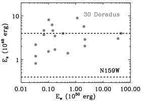
Figure 18: Left: $E_{\rm s}$ of the final shock models (shown in Fig. 14) is presented along with $\sim$500 stars for which $E_{\rm w}$ estimates are available ($E_{\rm w}\geq 10^{50}$ erg as the red crosses, 10⁴⁹ erg $\leq$ $E_{\rm w}$ $<$ 10⁵⁰ erg as the orange circles, and $E_{\rm s}$ $<$ 10⁴⁹ erg as the blue triangles; Doran et al. 2013). The location of R136 is also indicated as the red circle. Right: $E_{\rm s}$ as a function of $E_{\rm w}$. The data points for 30 Doradus are shown in gray, while the range of $E_{\rm s}$ estimated by Lee et al. (2016) for N159W is overlaid as the black dashed line.

6.2.2 Low-velocity shocks

In the case where low-velocity shocks are the origin of the high thermal pressure in the CO-emitting regions, stellar winds from hot luminous stars could provide the required mechanical energy to drive the shocks. To examine such a possibility, we calculated the total energy dissipated by shocks ($E_{\rm s}$) using our constrained models in Sect. 5.3.3 (Lee et al. 2016 for details on the calculation) and compared it with the stellar wind energy ($E_{\rm w}$) of $\sim$500 W-R and OB-type stars from Doran et al. (2013) (Fig. 18 Left). For our comparison, the shock timescale of 0.1 Myr (typical time needed for the shocked medium to return to equilibrium) and the wind timescale of 2 Myr (average OB stellar lifetime) were assumed, essentially following Doran et al. (2013) and Lee et al. (2016). When considering $\sim$150 stars that fall into the 23 pixels where our shock solutions exist, we found that stellar winds from these stars can inject the total mechanical energy of $\sim$10⁵² erg, which would be sufficient to drive the low-velocity shocks dissipating $\sim$10⁵⁰ erg in the region. These total energies of $\sim$10⁵² erg and $\sim$10⁵⁰ erg were estimated by simply summing up $E_{\rm w}$ and $E_{\rm s}$ over the 23 pixels in our consideration. Interestingly, Fig. 18 Left shows that the shock and wind energy have contrasting spatial distributions: $E_{\rm s}$ varies smoothly across the region, while $E_{\rm w}$ is highly concentrated around R136. To quantify this difference, we then calculated $E_{\rm w}$ on a pixel-by-pixel basis by summing $E_{\rm w}$ values of all W-R and OB-type stars that fall into each FTS pixel and compared it to $E_{\rm s}$ (Fig. 18 Right). As we just discussed, Fig. 18 Right clearly demonstrates that $E_{\rm s}$ is relatively uniform with a factor of $\sim$10 variations, while $E_{\rm w}$ changes by a factor of $\sim$2000 ($E_{\rm w}$ $>$ 10⁵¹ erg coincides with R136 and its adjacent pixels). This highly concentrated distribution of $E_{\rm w}$ was also noted by Doran et al. (2013), i.e., 75% of the total wind luminosity is contained within 20 pc of R136, and suggests that stellar winds are likely not the main driver of the low-velocity shocks.

In addition to stellar winds from hot luminous stars, SNe can inject a large amount of mechanical energy into the surrounding ISM ($\sim$10⁵¹ erg per SNe; e.g., Hartmann 1999). So far 59 SNRs have been identified in the LMC (Maggi et al. 2016), and 30 Doradus harbors only one SNR, N157B at ($\alpha$, $\delta$)_J2000 = (05^h37^m47^s, $-69^{\circ}$10^′20^′′) (Chen et al. 2006). Considering that 30 Doradus hosts $\sim$25% of the massive stars in the LMC (Kennicutt & Hodge 1986) and core-collapsed SNRs closely follow active star formation (25 such SNRs in the LMC; Maggi et al. 2016), however, we would expect to find more SNRs in 30 Doradus and roughly estimate the expected number of 25 $\times$ 0.25 $\sim$ 6 SNRs (which could have been missed previously due to their low surface brightness and/or the crowdedness in the 30 Doradus region). While our estimate is uncertain, it is indeed consistent with the roughly half-dozen high-velocity ionized bubbles in 30 Doradus (likely blown up by SNe; e.g., Chu & Kennicutt 1994) and implies that SNe could provide sufficient energy to drive the low-velocity shocks. But again, as in the case of stellar winds, the relatively uniform distribution of $E_{\rm s}$ would be difficult to explain in the framework of SNe-driven shocks.

Our results so far suggest that the low-velocity shocks in 30 Doradus likely originate from non-stellar sources. This conclusion is also consistent with the fact that 30 Doradus and N159W have comparable $E_{\rm s}$ on $\sim$10 pc scales (our FTS pixel size; Fig. 18 Right) despite a large difference in the number of massive young stars: $\sim$1100 in 30 Doradus vs. $\sim$150 in N159W (Fariña et al. 2009; Doran et al. 2013). The comparable $E_{\rm s}$ values between 30 Doradus and N159W would in turn suggest that large-scale processes ($\gtrsim$ 600 pc; distance between 30 Doradus and N159W) are likely the major source of the low-velocity shocks, and the kpc-scale injection of significant energy into the Magellanic Clouds has been indeed suggested by previous power spectrum analyses (e.g., Elmegreen et al. 2001; Nestingen-Palm et al. 2017). One of the possible processes for energy injection on kpc-scales is the complicated interaction between the Milky Way and the Magellanic Clouds. While the dynamics of the entire Magellanic System (two Magellanic Clouds and gaseous structures surrounding them, i.e., the Stream, the Bridge, and the Leading Arm) is still a subject of active research, it has been well known that the southeastern H i overdensity region where 30 Doradus and N159W are located (Fig. 1) is strongly perturbed (e.g., Luks & Rohlfs 1992) and likely influenced by tidal and/or ram-pressure stripping between the Milky Way and the Magellanic Clouds (e.g., D’Onghia & Fox 2016). Such an energetic interplay between galaxies can deposit a large amount of mechanical energy, which would then cascade down to small scales and low velocities, as witnessed in both local and high-redshift interacting systems (e.g., Appleton et al. 2017; Falgarone et al. 2017).

Finally, we note that low-velocity shocks would be pervasive in the LMC if they indeed arise from kpc-scale processes. These shocks would have a negligible impact on the low-$P$ PDR component in 30 Doradus though, since the shocks would compress only a fraction of this diffuse and extended component, e.g., line-of-sight depth of $\sim$10^-2 pc and $\sim$6 pc for the high-$P$ shock and low-$P$ PDR component respectively (Sect. 6.1).

6.3 CO SLEDs as a probe of the excitation mechanisms of warm molecular gas

So far we analyzed the observed CO SLEDs of 30 Doradus with an aim of examining the excitation mechanisms of warm molecular gas in star-forming regions, and our results clearly show that CO SLEDs alone cannot differentiate heating sources. For example, the observed CO SLEDs significantly change across 30 Doradus (Sect. 4.2), e.g., $J_{\rm p}$ ranging from 6–5 to 10–9 and $\alpha$ ranging from $\sim$0.4 to $\sim$1.8, and our PDR and shock modeling suggest that these varying CO SLEDs mostly reflect the changes in physical conditions (e.g., temperature and density), rather than underlying excitation mechanisms. The fact that N159W has systematically different CO SLEDs (e.g., $J_{\rm p}$ = 4–3 to 7–6 and $\alpha$ = 0.3–0.7; Lee et al. 2016), yet likely shares the same excitation mechanism as 30 Doradus, also supports our conclusion. In addition to CO lines, complementary observational constraints, e.g., fine-structure lines, FIR luminosity, and properties of massive young stars, were then found to be highly essential to examine the excitation mechanisms in detail and evaluate their feasibility. All in all, our study demonstrates that one should take a comprehensive approach when interpreting multi-transition CO observations in the context of probing the excitation sources of warm molecular gas (e.g., Mashian et al. 2015; Indriolo et al. 2017; Kamenetzky et al. 2017).

Another key result from our work is the crucial role of shocks in CO heating. As described in Sect. 1, both Galactic and extragalactic studies have highlighted the importance of mechanical heating for CO, and our N159W and 30 Doradus analyses show that mechanical heating by low-velocity shocks ($\sim$10 km s^-1) is indeed a major contributor to the excitation of molecular gas on $\sim$10 pc scales. What remains relatively uncertain is the source of shocks. While we concluded that low-velocity shocks in N159W and 30 Doradus likely originate from large-scale processes such as the complex interaction between the Milky Way and the Magellanic Clouds, this hypothesis should be verified by observing independent shock tracers, e.g., SiO and H₂ transitions, throughout the LMC. Such observations would be possible with current and upcoming facilities, e.g., ALMA, SOFIA, and JWST, providing insights into the injection and dissipation of mechanical energy in the ISM. These observations will also further test our tentative rejection of UV photons as the main heating source for CO (Sect. 6.2.1).

7 Summary

In this paper, we present Herschel SPIRE FTS observations of 30 Doradus, the most extreme starburst region in the Local Universe harboring more than 1000 massive young stars. To examine the physical conditions and excitation mechanisms of molecular gas, we combined the FTS CO observations (CO $J$=4–3 to $J$=13–12) with other tracers of gas and dust and analyzed them on 42^′′ or $\sim$10 pc scales using the state-of-the-art Meudon PDR and Paris-Durham shock models. Our main results are as follows.

1. In our FTS observations, important cooling lines in the ISM, such as CO rotational transitions (from $J$=4–3 to $J$=13–12), [C i] 370 $\mu$m, and [N ii] 205 $\mu$m, were clearly detected.

2. We constructed CO SLEDs on a pixel-by-pixel basis by combining the FTS observations with ground-based CO(1–0) and CO(3–2) data and found that the CO SLEDs vary considerably across 30 Doradus. These variations include the changes in the peak transition $J_{\rm p}$ (from $J$=6–5 to $J$=10–9), as well as in the slope characterized by the high-to-intermediate $J$ ratio $\alpha$ (from $\sim$0.4 to $\sim$1.8).

3. To evaluate the impact of UV photons on CO, we performed Meudon PDR modeling and showed that CO emission in 30 Doradus could arise from $\sim$0.7–2 pc scale PDR clumps with $A_{V}$ $\gtrsim$ 5 mag, $P/k_{\rm B}$ $\sim$ 10⁸–10⁹ K cm^-3, and $G_{\rm UV}$ $\sim$ 10³–10⁵. Interestingly, these PDR clumps are quite faint in [C ii] 158 $\mu$m and FIR dust continuum emission, and we found that another PDR component with lower $A_{V}$ $\sim$ 2 mag, $P/k_{\rm B}$ $\sim$ a few (10⁴–10⁵) K cm^-3, and $G_{\rm UV}$ $\sim$ a few (10²–10³) (filling a large fraction of $\sim$10 pc-size FTS pixels) is required to explain the observed fine-structure lines ([C ii] 158 $\mu$m, [C i] 370 $\mu$m, and [O i] 145 $\mu$m) and FIR luminosity. The constrained properties of the high-$P$ PDR clumps, however, are not consistent with what we would expect based on the stellar content of 30 Doradus, and we thus tentatively concluded that UV photons are likely not the primary heating source for CO.

4. Based on the observed X-ray and $\gamma$-ray properties of 30 Doradus, we concluded that X-rays and cosmic-rays likely play a minor role in CO heating.

5. Our Paris-Durham shock modeling showed that the observed CO SLEDs of 30 Doradus can be reproduced by low-velocity C-type shocks with $n_{\rm pre}$ $\sim$ 10⁴–10⁶ cm^-3 and $\varv_{\rm s}$ $\sim$ 5–10 km s^-1. The shock-compressed ($P/k_{\rm B}$ $\sim$ 10⁷–10⁸ K cm^-3) CO-emitting clumps on $\sim$0.7–2 pc scales are likely well-shielded from dissociating UV photons and embedded within the low-$P$ PDR component that emits brightly in [C ii] 158 $\mu$m, [C i] 370 $\mu$m, [O i] 145 $\mu$m, and FIR continuum emission. Considering the properties of massive young stars in 30 Doradus, we excluded the stellar origin of low-velocity shocks and concluded that the shocks are likely driven by large-scale processes such as the interaction between the Milky Way and the Magellanic Clouds.

6. Our analyses suggest that the significant variations in the observed CO SLEDs of 30 Doradus mostly reflect the changes in physical conditions (e.g., temperature and density), rather than underlying excitation mechanisms. This implies that the shape of CO SLEDs alone cannot be used as a probe of heating sources.

While large-scale low-velocity shocks were suggested as the dominant heating source of CO in 30 Doradus, we note that our conclusion was based on $\sim$10 pc scale analyses. As Indriolo et al. (2017) pointed out, CO SLEDs strongly depend on spatial scales, and how the spatial scale of CO observations affects the interpretation of heating sources is currently unclear. For a more comprehensive picture on the nature of warm molecular gas in individual star-forming regions, it would hence be critical to analyze high spatial and spectral resolution CO observations over a large area in combination with complementary constraints, e.g., PDR and shock tracers, as well as stellar properties.

Appendix A FTS data

In Fig. 19, we present the FTS CO, [C i] , and [N ii] integrated intensity images of 30 Doradus. All images are at 42^′′ resolution ($\sim$10 pc at the LMC distance) with a pixel size of 30^′′. In each image, the spectra of individual pixels are overlaid in red (detections with $S/N_{\rm s}>5$) and blue (non-detections with $S/N_{\rm s}\leq 5$). These spectra are plotted with the same $x$- and $y$-axis ranges (in GHz and 10^-18 W m^-2 Hz^-1 sr^-1), which can be found in the top left corner of the image with an example spectrum. The example spectrum is from the pixel that was observed with the central SLWC3 and SSWD4 detectors of the first jiggle position of the Obs. ID = 1342219550 (yellow and orange crosses).

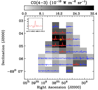
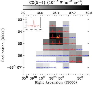
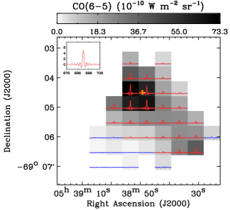
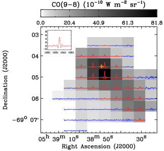
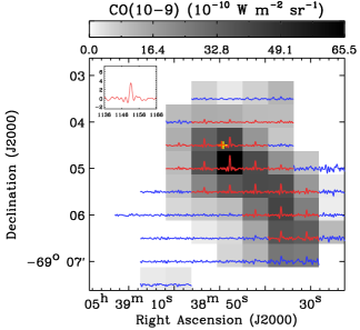
Figure 19: FTS CO, [C i] , and [N ii] integrated intensity images of 30 Doradus. See Appendix A for details on these figures.

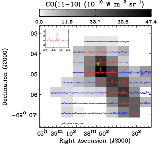
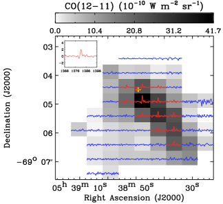
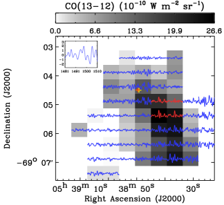
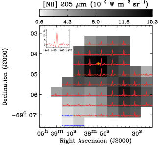
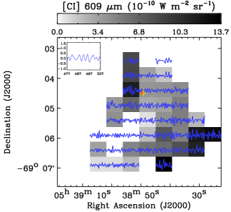
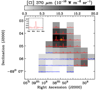
Figure 20: (continued)

Appendix B Stellar UV radiation field

To derive the stellar UV radiation field $G_{\rm stars}$ of 30 Doradus, we essentially followed Chevance et al. (2016) and provide here a summary of our derivation. First, we cross-matched the catalogs of massive stars (W-R and OB-type stars) published by Crowther & Dessart (1998), Selman et al. (1999), and Doran et al. (2013) and extracted the temperatures of $\sim$1.3 $\times$ 10⁴ sources. The catalog by Doran et al. (2013) was used as our main reference when possible, since it likely provides more reliable estimates of stellar properties based on spectroscopic observations, and the other two catalogs were used to complement it. We then integrated a blackbody from 912 Å to 2400 Å for each star to be consistent with the definition of $G_{\rm UV}$ in the Meudon PDR model and calculated $G_{\rm stars}$ for each 30^′′-size pixel of a 5^′ $\times$ 5^′ image (matching the coverage and pixel size of the FTS maps) by assuming that all the stars lie on the same plane as R136 and summing the UV fluxes of the stars. The derived $G_{\rm stars}$ on the plane of R136 is presented in Fig. 7 and can be considered as the maximum incident UV radiation field we expect, since no absorption was taken into account. While absorption by dust would have an important impact on the derivation of $G_{\rm stars}$, estimating absorption is currently not straightforward due to the lack of information on the location of absorbers.

Compared to Chevance et al. (2016), the only difference is our usage of the catalog by Doran et al. (2013). This results in $\sim$50% stronger UV radiation field on average, suggesting that a factor of two or so uncertainty could arise from the selection of stellar catalogs. Another source of uncertainty is our assumption of the stellar distribution, and we examined this issue by deriving $G_{\rm stars}$ with a random three-dimensional distribution of the stars. We then found that the assumption of the stars on the same plane tends to underestimate $G_{\rm stars}$ by up to $\sim$30%.

Appendix C PDR contribution to FIR emission

FIR emission can originate not only from PDRs (neutral gas), but also from H ii regions (ionized gas). To be properly compared to the predictions from the Meudon PDR model, our $L_{\rm FIR}$ derived from dust SED modeling (Sect. 3.5) then needs to be corrected for the contribution from the ionized medium. To do so, we used the PAH and [O iii] 88 $\mu$m images from Chevance et al. (2016) and performed the following steps (essentially what Chevance et al. 2016 did, but on 42^′′ scales). First, we assumed that PAH and [O iii] 88 $\mu$m emission trace PDRs and H ii regions respectively and adopted a linear relation $L_{\rm FIR}$ = $\alpha L_{\rm PAH}+\beta L_{\rm[O\leavevmode\nobreak\ \textsc{iii}]}$. The coefficients ($\alpha$, $\beta$) = (4.6, 8.8) were then derived by fitting a multiple regression model to all available pixels, and the PDR-only component of $L_{\rm FIR}$ was estimated as $L_{\rm FIR}^{\rm PDR}$ = $L_{\rm FIR}-\beta L_{\rm[O\leavevmode\nobreak\ \textsc{iii}]}$. Note that our analysis is based on the assumption that the PAH-to-dust mass ratio does not change in the PDRs and drops to zero in the H ii regions.

This $L_{\rm FIR}^{\rm PDR}$ is what we used as an input for PDR modeling in Sect. 5.1, and we assigned 30% of $L_{\rm FIR}^{\rm PDR}$ as 1$\sigma$ uncertainties, considering the simple empirical relation we adopted. The resulting $L_{\rm FIR}^{\rm PDR}$ shows a good agreement with Chevance et al. (2016), e.g., the PDR contribution to $L_{\rm FIR}$ ranges from $\sim$40% to $\sim$80% across the 30 Doradus region ($\sim$30% to $\sim$90% in Chevance et al. 2016).

Appendix D Comparison with Chevance et al. (2016)

As described in Sect. 2.2, Chevance et al. (2016) recently studied the properties of PDRs in 30 Doradus on 12^′′ scales by performing Meudon PDR modeling of [C ii] 158 $\mu$m, [O i] 145 $\mu$m, and FIR emission. Since we employed essentially the same datasets and modeling approach for our analyses (Sect. 5.1.3), it is important to double-check that our results are indeed consistent with those in Chevance et al. (2016).

As for the spatial distributions of the PDR parameters (e.g., peak locations of $P$, $G_{\rm UV}$, and $\Omega$), we found that our results are consistent with Chevance et al. (2016). However, a comparison of the absolute values showed a large discrepancy, as can be seen in Fig. 21. Specifically, we noticed that our $P$ and $G_{\rm UV}$ distributions primarily trace the lower part of the Chevance et al. (2016) histograms, while the opposite is the case for $\Omega$.

This large discrepancy in the absolute values of the PDR parameters could result from several differences between the two studies, e.g., resolution (42^′′ vs. 12^′′), spatial coverage (our maps are smaller), and slightly inconsistent PDR models (version 1.5.2 with $A_{V}$ $\sim$ 2 mag vs. version 1.6.0 with $A_{V}$ = 3 mag). Among these possibilities, we probed the impact of different resolutions by performing Meundon PDR modeling of [C ii] 158 $\mu$m, [O i] 145 $\mu$m, and FIR emission for one pixel (chosen as the one where the $G_{\rm UV}$ distribution in Chevance et al. (2016) peaks), but on 12^′′ scales. For this purpose, we used the same model grid with $A_{V}$ = 2 mag, as well as the same fitting method, as in Sect. 5.1.3 and constrained $P/k_{\rm B}$ = 7 $\times$ 10⁵ K cm^-3, $G_{\rm UV}$ = 3 $\times$ 10⁴, and $\Omega$ = 0.7. These results are in good agreement with what Chevance et al. (2016) estimated ($P/k_{\rm B}$ = 10⁶ K cm^-3, $G_{\rm UV}$ = 3 $\times$ 10⁴, and $\Omega$ = 0.5), essentially suggesting that the discrepancy between our study and Chevance et al. (2016) mostly results from the difference in the angular resolution. As Chevance et al. (2016) pointed out as well, utilizing lower resolution data skews the PDR solutions toward lower $P$ and $G_{\rm UV}$, since the intensities measured on larger scales tend to be more dominated by the emission from diffuse regions with less UV illumination.

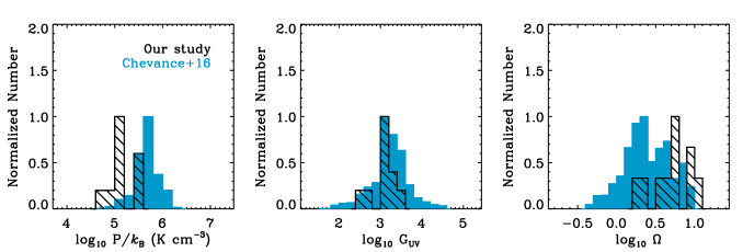
Figure 21: Comparison with Chevance et al. (2016). The normalized histograms of the PDR parameters in our study (42^′′ scales) and Chevance et al. (2016) (12^′′ scales) are shown in black (hatched) and blue (solid) respectively ($P/k_{\rm B}$, $G_{\rm UV}$, and $\Omega$ on the right, middle, and left panels).

Appendix E Comparison with Okada et al. (2019)

Recently, Okada et al. (2019) presented an independent study on CO (CO $J$=2–1, 3–2, 4–3, and 6–5, as well as ¹³CO $J$=3–2; observed with APEX) and fine-structure lines ([C ii] 158 $\mu$m, [C i] 609 $\mu$m and 370 $\mu$m, and [O i] 63 $\mu$m and 145 $\mu$m; observed with APEX and SOFIA) in 30 Doradus. Among the observed transitions, CO, ¹³CO, [C ii] and [C i] were mapped over an area that is comparable to our FTS coverage, while [O i] was obtained for selected positions only. This study based on high spatial ($\sim$6^′′ to $\sim$30^′′) and spectral ($\sim$1 km s^-1) resolution data is complementary to our work, and we provide here a summary of it.

First of all, their high resolution data clearly demonstrate the complexity of the neutral ISM in 30 Doradus. For example, the authors found that CO, ¹³CO, and [C i] spectra are similar, while [C ii] 158 $\mu$m shows a wider linewidth and/or additional velocity components. In addition, [O i] spectra match CO spectra at some locations, but they are more similar to [C ii] 158 $\mu$m profiles at other locations. In terms of spatial distribution, [C ii] 158 $\mu$m and CO $J$=4–3 show relatively similar structures, except for several mismatching peaks.

The complexity of the neutral ISM in 30 Doradus was also manifested in KOSMA-$\tau$ PDR modeling by Okada et al. (2019). The KOSMA-$\tau$ model calculates the thermal and chemical structures of a PDR as the Meudon PDR model does, but with a different geometry of the medium. Specifically, while the Meudon PDR model considers a plane-parallel slab of gas and dust, the KOSMA-$\tau$ model assumes an ensemble of clumps with a power-law mass spectrum $dN/dM$ $\propto$ $M^{-\alpha}$ ($\alpha$ = 1.8 was used in Okada et al. 2019) to take into account the clumpiness of the ISM. Line and continuum intensities are then estimated by adding the contribution from each clump for a model grid of three parameters, total mass ($M_{\rm tot}$), average gas density ($\overline{n}$), and UV radiation field ($G^{\prime}_{\rm UV}$). For more details on the KOSMA-$\tau$ PDR model, we refer to Stoerzer et al. (1996) and Röllig et al. (2006). While we cannot make a direct comparison with Okada et al. (2019) due to systematic differences in PDR modeling (e.g., input parameters and modeling approach), our results are essentially consistent in a way that both our study and Okada et al. (2019) show that one ISM component is not sufficient to analyze 30 Doradus. For example, Okada et al. (2019) modeled their observed transitions along with dust continuum emission for 30Dor-10 at ($\alpha$, $\delta$)_J2000 = (05^h38^m48.8^s, $-69^{\circ}$04^′42.1^′′) and found that CO and [C i] are relatively well reproduced, while [C ii] and [O i] are overestimated by a factor of a few. This best-fit KOSMA-$\tau$ model, however, predicts the CO SLED to be flat already around at $J$=6–5, suggesting that the gas is not warm enough ($J_{\rm p}$ = 9–8 in our FTS observations). The constrained UV radiation field ($\sim$200 Draine fields) is indeed weaker than what we estimated for the low- and high-$P$ PDR components ($\sim$3 $\times$ 10³ Draine fields). In addition, the large beam filling factor of $\gtrsim$ 1 is not consistent with what the ALMA CO(2–1) observations suggest (Indebetouw et al. 2013). All in all, both our study and Okada et al. (2019) highlight that many high resolution tracers of gas and dust are required to build a consistent picture of the multi-phase, multi-component ISM in complex regions like 30 Doradus.