Power up! Robust Graph Convolutional Network via Graph Powering

Abstract

Graph convolutional networks (GCNs) are powerful tools for graph-structured data. However, they have been recently shown to be vulnerable to topological attacks. To enhance adversarial robustness, we go beyond spectral graph theory to robust graph theory. By challenging the classical graph Laplacian, we propose a new convolution operator that is provably robust in the spectral domain and is incorporated in the GCN architecture to improve expressivity and interpretability. By extending the original graph to a sequence of graphs, we also propose a robust training paradigm that encourages transferability across graphs that span a range of spatial and spectral characteristics. The proposed approaches are demonstrated in extensive experiments to simultaneously improve performance in both benign and adversarial situations.

Introduction

Graph convolutional networks (GCNs) are powerful extensions of convolutional neural networks (CNN) to graph-structured data. Recently, GCNs and variants have been applied to a wide range of domains, achieving state-of-the-art performances in social networks (Kipf and Welling 2017; Chang et al. 2020a; Gu et al. 2020), traffic prediction (Rahimi, Cohn, and Baldwin 2018), recommendation systems (Ying et al. 2018; Guan et al. 2021), applied chemistry and biology (Kearnes et al. 2016; Fout et al. 2017), and natural language processing (Atwood and Towsley 2016; Hamilton, Ying, and Leskovec 2017; Bastings et al. 2017; Marcheggiani and Titov 2017), just to name a few (Zhou et al. 2018; Wu et al. 2019).

GCNs belong to a family of spectral methods that deal with spectral representations of graphs (Zhou et al. 2018; Wu et al. 2019). A fundamental ingredient of GCNs is the graph convolution operation defined by the graph Laplacian in the Fourier domain:

$$\bm{g}_{\bm{\theta}}\star\bm{x}\coloneqq\hat{\bm{g}}_{\bm{\theta}}(\bm{L})\bm{x},$$ (1)

where $\bm{x}\in\mathbb{R}^{n}$ is the graph signal on the set of vertices $\mathcal{V}$ and $\hat{\bm{g}}_{\bm{\theta}}$ is a spectral function applied to the graph Laplacian $\bm{L}\coloneqq\bm{D}-\bm{A}$ (where $\bm{D}$ and $\bm{A}$ are the degree matrix and the adjacency matrix, respectively). Because this operation is computational intensive for large graphs and non-spatially localized (Bruna et al. 2014), early attempts relied on a parameterization with smooth coefficients (Henaff, Bruna, and LeCun 2015) or a truncated expansion in terms of of Chebyshev polynomials (Hammond, Vandergheynst, and Gribonval 2011). By further restricting the Chebyshev polynomial order by 2, the approach in (Kipf and Welling 2017) referred henceforth as the vanilla GCN pushed the state-of-the-art performance of semi-supervised learning. The network has the following layer-wise update rule:

$$\bm{H}^{(l+1)}\coloneqq\psi\left(\mathcal{A}\bm{H}^{(l)}\bm{W}^{(l)}\right),$$ (2)

where $\bm{H}^{(l)}$ is the $l$-th layer hidden state (with $\bm{H}^{(1)}\coloneqq\bm{X}$ as nodal features), $\bm{W}^{(l)}$ is the $l$-th layer weight matrix, $\psi$ is the usual point-wise activation function, and $\mathcal{A}$ is the convolution operator chosen to be the degree weighted Laplacian with some slight modifications (Kipf and Welling 2017). Subsequent GCN variants have different architectures, but they all share the use of the Laplacian matrix as the convolution operator (Zhou et al. 2018; Wu et al. 2019).

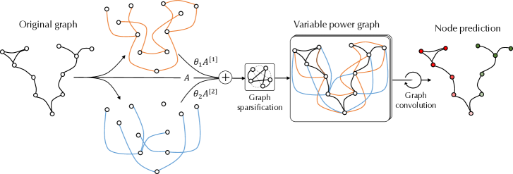
Figure 1: From the original graph, we generate a series of graphs, which are weighted by parameters of influence strengths, sparsified, and eventually combined to form a variable power graph.

Why Not Graph Laplacian?

Undoubtedly, the Laplacian operator (and its variants, e.g., normalized/powered Laplacian) plays a central role in spectral theory, and is a natural choice for a variety of spectral algorithms such as principal component analysis, clustering and linear embeddings (Chung and Graham 1997; Belkin and Niyogi 2002). So what can be problematic?

From a spatial perspective, GCNs with $d$ layers cannot acquire nodal information beyond its $d$-distance neighbors; hence, it severely limits its scope of data fusion. Recent works (Lee et al. 2018; Abu-El-Haija et al. 2018, 2019; Wu et al. 2019) alleviated this issue by directly powering the graph Laplacian.

From a spectral perspective, one could demand better spectral properties, given that GCN is fundamentally a particular (yet effective) approximation of the spectral convolution (1). A key desirable property for generic spectral methods is known as “spectral separation,” namely the spectrum should comprise a few dominant eigenvalues whose associated eigenvectors reveal the sought structure in the graph. A well-known prototype is the Ramanujan property, for which the second leading eigenvalue of a $r$-regular graph is no larger than $2\sqrt{r-1}$, which is also enjoyed asymptotically by random $r$-regular graphs (Friedman 2004) and Erdős-Rényi graphs that are not too sparse (Feige and Ofek 2005). In a more realistic scenario, consider the stochastic block model (SBM), which attempts to capture the essence of many networks, including social graphs, citation graphs, and even brain networks (Holland, Laskey, and Leinhardt 1983).

Definition 1 (Simplified stochastic block model).

The graph $\mathcal{G}$ with $n$ nodes is drawn under SBM$(n,k,a_{\text{intra}},a_{\text{inter}})$ if the nodes are evenly and randomly partitioned into $k$ communities, and nodes $i$ and $j$ are connected with probability ${a_{\text{intra}}}/{n}\in[0,1]$ if they belong to the same community, and ${a_{\text{inter}}}/{n}\in[0,1]$ if they are from different communities.

It turns out that for community detection, the top $k$ leading eigenvectors of the adjacency matrix $\bm{A}$ play an important role. In particular, for the case of 2 communities, spectral bisection algorithms simply take the second eigenvector to reveal the community structure. This can be also seen from the expected adjacency matrix $\mathbb{E}[\bm{A}]$ under SBM$(n,2,a_{\text{intra}},a_{\text{inter}})$, which is a rank-2 matrix with the top eigenvalue $\tfrac{1}{2}(a_{\text{intra}}+a_{\text{inter}})$ and eigenvector $\bm{1}$, and the second eigenvalue $\tfrac{1}{2}(a_{\text{intra}}-a_{\text{inter}})$ and eigenvector $\bm{\sigma}$ such that $\sigma_{i}=1$ if $i$ is in community 1 and $\sigma_{i}=-1$ otherwise. More generally, the second eigenvalue is of particular theoretical interests because it controls at the first order how fast heat diffuses through graph, as depicted by the discrete Cheeger inequality (Lee, Gharan, and Trevisan 2014).

While one would expect taking the second eigenvector of the adjacency matrix suffices, it often fails in practice (even when it is theoretically possible to recover the clusters given the signal-to-noise ratio). This is especially true for sparse networks, whose average nodal degrees is a constant that does not grow with the network size. This is because the spectrum of the Laplacian or adjacency matrix is blurred by “outlier” eigenvalues in the sparse regime, which is often caused by high degree nodes (Kaufmann, Bonald, and Lelarge 2016). Unsurprisingly, powering the Laplacian would be of no avail, because it does not change the eigenvectors or the ordering of eigenvalues. In fact, those outliers can become more salient after powering, thereby weakening the useful spectral signal even further. Besides, pruning the largest degree nodes in the adjacency matrix or normalizing the Laplacian cannot solve the issue. To date, the best results for pruning does not apply down to the theoretical recovery threshold (Coja-Oghlan 2010; Mossel, Neeman, and Sly 2012; Le, Levina, and Vershynin 2015); either outliers would persist or one could prune too much that the graph is destroyed. As for normalized Laplacian, it may overcorrect the large degree nodes, such that the leading eigenvectors would catch the “tails” of the graph, i.e., components weakly connected to the main graph. See the Appendix for an experimental illustration.

In summary, graph Laplacian may not be the ideal choice due to its limited spatial scope of information fusion, and its undesirable artefacts in the spectral domain.

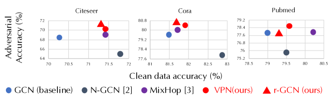
Figure 2: Our proposed framework can improve both clean and adversarial (10% attack by $\mathcal{A}_{DW_{3}}$ (Bojchevski and Günnemann 2019)) accuracy for semi-supervised learning benchmarks.

If Not Laplacian, Then What?

In searching for alternatives, potential choices are many, so it is necessary to clarify the goals. In view of the aforementioned pitfalls of the graph Laplacian, one would naturally ask the question:

Can we find an operator that has wider spatial scope, more robust spectral properties, and is meanwhile interpretable and can increase the expressive power of GCNs?

From a perspective of graph data analytics, this question gauges how information is propagated and fused on a graph, and how we should interpret “adjacency” in a much broader sense. An image can be viewed as a regular grid, yet the operation of a CNN filter goes beyond the nearest pixel to a local neighborhood to extract useful features. How to draw an analogy to graphs?

From a perspective of robust learning, this question sheds light on the basic observation that real-world graphs are often noisy and even adversarial. The nice spectral properties of a graph topology can be lost with the presence or absence of edges. What are some principled ways to robustify the convolution operator and graph embeddings?

In this paper, we propose a graph learning paradigm that aims at achieving this goal, as illustrated in Figure 1. The key idea is to generate a sequence of graphs from the given graph that capture a wide range of spectral and spatial behaviors. We propose a new operator based on this derived sequence.

Definition 2 (Variable power operator).

Consider an unweighted and undirected graph $\mathcal{G}$. Let $\bm{A}^{[k]}$ denote the $k$-distance adjacency matrix, i.e., $\big{[}\bm{A}^{[k]}\big{]}_{ij}=1$ if and only if the shortest distance (in the original graph) between nodes $i$ and $j$ is $k$. The variable power operator of order $r$ is defined as:

$$\bm{A}^{(r)}_{\bm{\theta}}=\sum_{k=0}^{r}\theta_{k}\bm{A}^{[k]},$$ (3)

where ${\bm{\theta}}\coloneqq(\theta_{0},\ldots,\theta_{r})$ is a set of parameters.

Clearly, $\bm{A}^{(r)}_{\bm{\theta}}$ is a natural extension of the classical adjacency matrix (i.e., $r=1$ and $\theta_{0}=\theta_{1}=1$). With power order $r>1$, one can increase the spatial scope of information fusion on the graph when applying the convolution operation. The parameters $\theta_{k}$ also has a natural explanation—the magnitude and the sign of $\theta_{k}$ can be viewed as “global influence strength” and “global influence propensity” at distance $k$, respectively, which also determines the participation factor of each graph in the sequence in the aggregated operator.

Furthermore, we provide some theoretical justification of the proposed operator by establishing the following asymptotic property of spectral separation under the important SBM setting, which is, nevertheless, not enjoyed by the classical Laplacian operator or its normalized or powered versions. (All proofs are given in the Appendix.)

Theorem 3 (Asymptotic spectral separation of variable power operator).

Consider a graph $\mathcal{G}$ drawn from SBM$(n,2,a_{\text{intra}},a_{\text{inter}})$. Assume that the signal-to-noise ratio $\xi_{2}^{2}/\xi_{1}>1$, where $\xi_{1}=\tfrac{1}{2}(a_{\text{intra}}+a_{\text{inter}})$ and $\xi_{2}=\tfrac{1}{2}(a_{\text{intra}}-a_{\text{inter}})$ (c.f., (Decelle et al. 2011)). Suppose $r$ is on the order of $c\log(n)$ for a constant $c$, such that $c\log(\xi_{1})<1/4$. Given nonvanishing $\theta_{k}$ for $k>r/2$, the variable power operator $\bm{A}^{(r)}_{\bm{\theta}}$ has the following spectral properties: (i) the leading eigenvalue is on the order of $\Theta\left(\|{\bm{\theta}}\|_{1}\xi_{1}^{r}\right)$, the second leading eigenvalue is on the order of $\Theta\left(\|{\bm{\theta}}\|_{1}\xi_{2}^{r}\right)$, and the rest are bounded by $\|{\bm{\theta}}\|_{1}n^{\epsilon}\xi_{1}^{r/2}O(\log(n))$ for any fixed $\epsilon>0$; and (ii) the two leading eigenvectors are sufficient to recover the two communities asymptotically (i.e., as $n$ goes to infinity).

Theorem 3 is the weighted analogue of Theorem 2 from (Abbe et al. 2018). Intuitively, the above theoretical result suggests that the variable power operator is able to “magnify” benign signals from the latent graph structure while “suppressing” noises due to random artefacts. This is expected to improve spectral methods in general, especially when the benign signals tend to be overwhelmed by noises. For the rest of the paper, we will apply this insight to propose a robust graph learning paradigm in Section Graph Augmentation: Robust Training Paradigm, as well as a new GCN architecture in Section From Fixed to Variable Power Network. We also provide empirical evidence of the gain from this theory in Section Experiments and conclude in Section Conclusion.

Related Works

Beyond nearest neighbors. Several works have been proposed to address the issue of limited spatial scope by powering the adjacency matrix (Lee et al. 2018; Wu et al. 2019; Li et al. 2019). However, simply powering the adjacency does not extract spectral gap and may even make the eigenspectrum more sensitive to perturbations. (Abu-El-Haija et al. 2018, 2019) also introduced weight matrices for neighbors at different distances. But this could substantially increase the risk of overfitting in the low-data regime and make the network vulnerable to adversarial attacks.

Robust spectral theory. The robustness of spectral methods has been extensively studied for graph partitioning/clustering (Li et al. 2007; Balakrishnan et al. 2011; Chaudhuri, Chung, and Tsiatas 2012; Amini et al. 2013; Joseph, Yu et al. 2016; Diakonikolas et al. 2019). Most recently, operators based on self-avoiding or nonbacktracking walks have become popular for SBM (Massoulié 2014; Mossel, Neeman, and Sly 2013; Bordenave, Lelarge, and Massoulié 2015), which provably achieve the detection threshold conjectured by (Decelle et al. 2011). Our work is partly motivated by the graph powering approach by (Abbe et al. 2018), which leveraged the result of (Massoulié 2014; Bordenave, Lelarge, and Massoulié 2015) to prove the spectral gap. The main difference with this line of work is that these operators are studied only for spectral clustering without incorporating nodal features. Our proposed variable power operator can be viewed as a kernel version of the graph powering operator (Abbe et al. 2018), thus substantially increasing the capability of learning complex nodal interactions while maintaining the spectral property.

Robust graph neural network. While there is a surge of adversarial attacks on graph neural networks (GNNs) (Dai et al. 2018; Zügner and Günnemann 2019; Bojchevski and Günnemann 2019; Chang et al. 2020b, 2021), very few methods have been proposed for defense (Sun et al. 2018). Existing works employed known techniques from computer vision (Szegedy et al. 2014; Goodfellow, Shlens, and Szegedy 2015; Szegedy et al. 2016), such as adversarial training with “soft labels” (Chen et al. 2019) or outlier detection in the hidden layers (Zhu et al. 2019), but they do not exploit the unique characteristics of graph-structured data. Importantly, our approach simultaneously improves performance in both the benign and adversarial tests, as shown in Figure 2 (details are presented in Section Experiments).

Graph Augmentation: Robust Training Paradigm

Exploration of the spectrum of spectral and spatial behaviors. Given a graph $\mathcal{G}$, consider a family of its powered graphs, $\left\{\mathcal{G}^{(2)},\ldots,\mathcal{G}^{(r)}\right\}$, where $\mathcal{G}^{(k)}$ is obtained by connecting nodes with distance less than or equal to $k$. This “graph augmentation” procedure is similar to “data augmentation”, because instead of limiting the learning on a single graph that is given, we artificially create a series of graphs that are closely related to each other in the spatial and spectral domains.

As we increase the power order, the graph also becomes more homogenized. In particular, it can help near-isolated nodes (i.e., low-degree vertices), since they become connected beyond their nearest neighbors. By comparison, simply raising the adjacency matrix to its $r$-th power will make them appear even more isolated, because it inadvertently promotes nodes with high degrees or nearby loops much more substantially as a result of feedback. Furthermore, the powered graphs can extract spectral gaps in the original graph despite local irregularities, thus boosting the signal-to-noise ratio in the spectral domain.

Transfer of knowledge from the powered graph sequence. Consider a generic learning task on a graph $\mathcal{G}$ with data $\mathcal{D}$. The loss function is denoted by $\ell(\mathcal{W};\mathcal{G},\mathcal{D})$ for a particular GCN architecture parametrized by $\mathcal{W}$. For instance, in semi-supervised learning, $\mathcal{D}$ consists of features and labels on a small set of nodes, and $\ell$ is the cross-entropy loss over all labeled examples. Instead of minimizing over $\ell(\mathcal{W};\mathcal{G},\mathcal{D})$ alone, we use all the powered graphs:

$$\ell(\mathcal{W};\mathcal{G},\mathcal{D})+\sum_{k=2}^{r}\alpha_{k}\ell(\mathcal{W};\mathcal{G}^{(k)},\mathcal{D}),$$ (r-GCN)

where $\alpha_{k}\geq 0$ gauges how much information one desires to transfer from powered graph $\mathcal{G}^{(k)}$ to the learning process. By minimizing the (r-GCN) objective, one seeks to optimize the network parameter $\mathcal{W}$ on multiple graphs simultaneously, which is beneficial in two ways: (i) in the low-data regime, like semi-supervised learning, it helps to reduce the variance to improve generalization and transferability; (ii) in the adversarial setting, it robustifies the network since it is more likely that the perturbed network is contained in the wider spectrum during training.

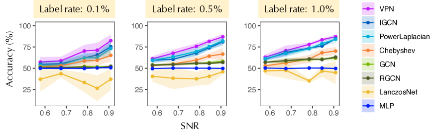
Figure 3: Comparison for SBM dataset. Shaded area indicates standard deviation over 10 runs.

Figure 4: Accuracy of first 100 frequency components of VPN (red) and adjacency matrix (blue).

From Fixed to Variable Power Network

By using the variable power operator illustrated in Figure 1, we substantially increase the search space of graph operators. The proposed operator also leads to a new family of graph algorithms with broader scope of spatial fusion and enhanced spectral robustness. As the power grows, the network eventually becomes dense. To manage this increased complexity and make the network more robust against adversarial attacks in the feature domain, we propose a pruning mechanism.

Graph sparsification. Given a graph $\mathcal{G}\coloneqq(\mathcal{V},\mathcal{E}^{[1]})$, consider its powered version $\mathcal{G}^{(r)}\coloneqq(\mathcal{V},\mathcal{E}^{(r)})$ and a sequence of intermediate graphs $\mathcal{G}^{[2]},\ldots,\mathcal{G}^{[r]}$, where $\mathcal{G}^{[k]}\coloneqq(\mathcal{V},\mathcal{E}^{[k]})$ is constructed by connecting two vertices if and only if the shortest distance is $k$ in $\mathcal{G}$. Clearly, $\{\mathcal{E}^{[k]}\}_{k=1}^{r}$ forms a partition of $\mathcal{E}^{(r)}$. For each node $i\in\mathcal{V}$, denote its $r$-neighborhood by $\mathcal{N}_{r}(i)\coloneqq\{j\in\mathcal{V}\mid d_{\mathcal{G}}(i,j)\leq r\}$, which is identical to the set of nodes adjacent to $i$ in $\mathcal{G}^{[r]}$. Next, for each edge within this neighborhood, we associate a value using some suitable distance metric $\phi$ to measure “aloofness.” For instance, it can be the usual Euclidean distance or correlation distance in the feature space. Based on this formulation, we prune an edge $e\coloneqq(i,j)$ in $\mathcal{E}^{(r)}$ if the value is larger than a threshold $\tau(i,j)$, and denote the edge set after pruning $\bar{\mathcal{E}}^{(r)}$. Then, we can construct a new sequence of sparsified graphs, $\overline{\mathcal{G}}^{[k]}$ with edge sets $\bar{\mathcal{E}}^{[k]}=\mathcal{E}^{[k]}\cap\bar{\mathcal{E}}^{(r)}$ and adjacency matrix $\bar{\bm{A}}^{[k]}$. Hence, the variable power operator is given by $\bar{\bm{A}}^{(r)}_{\bm{\theta}}=\sum_{k=0}^{r}\theta_{k}\bar{\bm{A}}^{[k]}$. Due to the influence of high-degree nodes in the spectral domain, one can adaptively choose the thresholds $\tau(i,j)$ to mitigate their effects. Specifically, we choose $\tau$ to be a small number if either $i$ or $j$ are nodes with high degrees, thereby making the sparsification more influential in densely connected neighborhoods than weakly connected parts.

Layer-wise update rule. To demonstrate the effectiveness of the proposed operator, we adopt the vanilla GCN strategy (2). Importantly, we replace the graph convolutional operator $\mathcal{A}$ with the variable power operator to obtain the variable power network (VPN):

$$\mathcal{A}=\bm{D}^{-\tfrac{1}{2}}(\bm{I}+\bar{\bm{A}}^{(r)}_{\bm{\theta}})\bm{D}^{-\tfrac{1}{2}},$$ (VPN)

where $D_{ii}=1+|\{j\in\mathcal{V}\mid d_{\mathcal{G}}(i,j)=1\}|$. The introduction of $\bm{I}$ is reminiscent of the “renormalization trick” (Kipf and Welling 2017), but it can be also viewed as a regularization strategy in this context, which is well-known to improve the spectral robustness (Amini et al. 2013; Joseph, Yu et al. 2016). This construction immediately increases the scope of data fusion by a factor of $r$.

Proposition 4.

By choosing $\mathcal{A}$ with (VPN) in the layer-wise update rule (2), the output at each node from a $L$-layer GCN depends on neighbors within $L*r$ hops.

Since we proved that the variable power operator has nice spectral separation in Theorem 3, VPN is expected to promote useful spectral signals from the graph topology (similar to the preservation of useful information in images (Jacobsen, Smeulders, and Oyallon 2018), our method preserves useful information in the graph topology). This claim is substantiated with the following proposition.

Proposition 5.

Given a graph with two hidden communities. Consider a 2-layer GCN architecture with layer-wise update rule (2). Suppose that $\mathcal{A}$ has a spectral gap. Further, assume that the leading two eigenvectors are asymptotically aligned with $\bm{1}$ and $\bm{\nu}$, i.e., the community membership vector, and that both are in the range of feature matrix $\bm{X}$. Then, there exists a configuration of $\bm{W}^{(1)}$ and $\bm{W}^{(2)}$ such that the GCN outputs can recover the community with high probability.

Experiments

The proposed methods are evaluated against several recent models, including vanilla GCN (Kipf and Welling 2017) and its variant PowerLaplacian where we simply replace the adjacent matrix with its powered version, three baselines using powered Laplacian IGCN (Li et al. 2019), SGC (Wu et al. 2019) and LNet (Liao et al. 2019), the recent method MixHop (Abu-El-Haija et al. 2019) which attempts to increase spatial scope fusion, as well as a state-of-the-art baseline and RGCN (Zhu et al. 2019), which is also aimed at improving the robustness of Vanilla GCN. All baseline methods on based on their public codes.

Revisiting Stochastic Block Model

SBM dataset. We generated a set of networks under SBM with 4000 nodes and parameters such that the SNRs range from 0.58 to 0.91. To disentangle the effects from nodal features with that from the spectral signal, we set the nodal features to be one-hot vectors. The label rates are 0.1%, 0.5% and 1%, the validation rate is 1%, and the rest of the nodes are testing points.

Performance. Since the nodal features do not contain any useful information, learning without topology such as multi-layer perceptron (MLP) is only as good as random guessing. The incorporation of graph topology improves classification performance—the higher the SNR (i.e., $\xi_{2}^{2}/\xi_{1}$, see Theorem 3), the higher the accuracy. Overall, as shown in Figure 3, the performance of the proposed method (VPN) is superior than other baselines, which either use Laplacian (GCN, Chebyshev, RGCN, LNet) or its powered variants (IGCN, PowerLaplacian).

Spectral separation and Fourier modes. From the eigenspectrum of the convolution operators, we see that the spectral separation property is uniquely possessed by VPN, whose first two leading eigenvectors carry useful information about the underlying communities: without the help of nodal features, the accuracy is 87% even with label rate of 0.5%. Let $\bm{\Phi}$ denote the Fourier modes of the the adjacency matrix or VPN, and $\bm{X}$ be the nodal features (i.e., identity matrix). We analyze the information from spectral signals (e.g., the $k$-th and $k+1$-th eigenvectors) by estimating the accuracy of an MLP with filtered nodal features, namely $\bm{\Phi}_{:,k:(k+1)}\bm{\Phi}_{:,k:(k+1)}^{\top}\bm{X}$, as shown in Figure 4. The accuracy reflects the information content in the frequency components. We see that the two leading eigenvectors of VPN are sufficient to perform classification, whereas those of the adjacency matrix cannot make accurate inferences.

Model	Citeseer	Cora	Pubmed
ManiReg (Belkin, Niyogi, and Sindhwani 2006)	$60.1$	$59.5$	$70.7$
SemiEmb (Weston et al. 2012)	$59.6$	$59.0$	$71.1$
LP (Zhu, Ghahramani, and Lafferty 2003)	$45.3$	$68.0$	$63.0$
DeepWalk (Perozzi, Al-Rfou, and Skiena 2014)	$43.2$	$67.2$	$65.3$
ICA (Lu and Getoor 2003)	$69.1$	$75.1$	$73.9$
Planetoid (Yang, Cohen, and Salakhutdinov 2016)	$64.7$	$75.7$	$77.2$
Vanilla GCN (Kipf and Welling 2017)	$70.3$	$81.5$	$79.0$
PowerLaplacian	$70.5$	$80.5$	$78.3$
IGCN(RNM) (Li et al. 2019)	$69.0$	$80.9$	$77.3$
IGCN(AR) (Li et al. 2019)	$69.3$	$81.1$	$78.2$
LNet (Liao et al. 2019)	$66.2\pm 1.9$	$79.5\pm 1.8$	$78.3\pm 0.3$
RGCN (Zhu et al. 2019)	$71.2\pm 0.5$	$\textbf{82.8}\pm 0.6$	$79.1\pm 0.3$
SGC (Wu et al. 2019)	$\textbf{71.9}\pm 0.1$	$81.0\pm 0.0$	$78.9\pm 0.0$
MixHop (Abu-El-Haija et al. 2019)	$71.4\pm 0.8$	$81.9\pm 0.4$	$\textbf{80.8}\pm 0.6$
r-GCN (this paper)	$71.3\pm 0.5$	$81.7\pm 0.2$	$79.3\pm 0.3$
VPN (this paper)	$\textbf{71.7}\pm 0.6$	$\textbf{82.3}\pm 0.3$	$\textbf{79.8}\pm 0.4$

Table 1: Results for semi-supervised node classification. We highlighted the best and the second best performances, where we broke the tie by choosing the one with the smallest standard deviation.

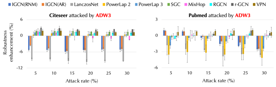
Figure 5: Robustness merit $\left(\text{accuracy}^{\text{post-attack}}_{\text{proposed-method}}-\text{accuracy}^{\text{post-attack}}_{\text{vanilla GCN}}\right)$ reported in percentage under $\mathcal{A}_{DW_{3}}$ attack. The error bar indicates standard deviation over 20 independent simulations.

Figure 6: Benign and adversarial accuracy as power order increases. Dahsed lines correspond to vanilla GCN.

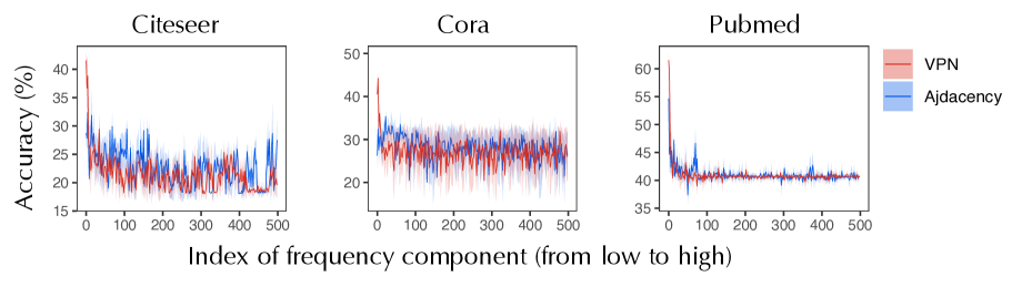
Figure 7: Accuracy of first 500 frequency components for VPN (red) and adjacency matrix (blue). The x axis corresponds to the index $k$ in $\bm{\Phi}_{:,k:(k+1)}\bm{\Phi}_{:,k:(k+1)}^{\top}\bm{X}$ for signal reconstruction.

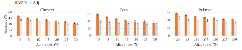
Figure 8: Accuracy of the leading frequency components in adversarial testing. We use $\widetilde{\bm{\Phi}}_{:,1:k}\widetilde{\bm{\Phi}}_{:,1:k}^{\top}\bm{X}$ as reconstructed nodal features for testing, where $k$ is 10 for Citeseer and 5 for Cora and Pubmed. Error bar indicates standard deviation over 10 runs.

Semi-supervised Node Classification

Experimental setup. We followed the setup of (Yang, Cohen, and Salakhutdinov 2016; Kipf and Welling 2017) for citation networks Citeseer, Cora and Pubmed (please refer to the Appendix for more details).

Graph powering order can influence spatial and spectral behaviors. Our theory suggests powering to the order of $\log(n)$; in practice, orders of 2 to 4 suffice (Figure 6). Here, we chose the power order to be 4 for r-GCN on Citeseer and Cora, and 3 for Pubmed, and reduced the order by 1 for VPN.

Performance. By replacing Laplacian with VPN, we see an immediate improvement in performance (Table 1). We also see that a succinct parametrization of the global influence relation in VPN is able to increase the expressivity of the network. For instance, the learned ${\bm{\theta}}$ at distances 2 and 3 for Citeseer are 3.15e-3 and 3.11e-3 with $p$-value less than 1e-5. This implies that the network tends to put more weights in closer neighbors.

Defense Against Evasion Attacks

To evaluate the robustness of the learned network, we considered the setting of evasion attacks, where the model is trained on benign data but tested on adversarial data.

Adversarial methods. Five strong global attack methods are considered, including DICE (Zügner and Günnemann 2019), $\mathcal{A}_{abr}$ and $\mathcal{A}_{DW_{3}}$ (Bojchevski and Günnemann 2019), Meta-Train and Meta-Self (Zügner and Günnemann 2019). We further modulated the severity of attack methods by varying the attack rate, which corresponds to the percentage of edges to be attacked.

Robustness evaluation. In general, both r-GCN and VPN are able to improve over baselines for the defense against evasion attacks, e.g., Figure 5 for the $\mathcal{A}_{DW_{3}}$ attack (detailed results for other attacks are listed in the Appendix). It can be also observed that the proposed methods are more robust in Citeseer and Cora than Pubmed. In addition to the low label rates, we conjectured that topological attacks are more difficult to defend for networks with prevalent high-degree nodes, because the attacker can bring in more irrelevant vertices by simply adding a link to the high-degree nodes.

Informative and robust low-frequency spectral signal. It has been observed by (Wu et al. 2019; Maehara 2019) that GCNs share similar characteristics of low-pass filters, in the sense that nodal features filtered by low-frequency Fourier modes lead to accurate classifiers (e.g., MLP). However, one key question left unanswered is how to obtain the Fourier modes. In their experiments, they derive it from the graph Laplacian. By using VPN to construct the Fourier modes, we show that the information content in the low-frequency domain can be improved.

More specifically, we first perform eigendecomposition of the graph convolutional operator (i.e., graph Laplacian or VPN) to obtain the Fourier modes $\bm{\Phi}$. We then reconstruct the nodal features $\bm{X}$ using only the $k$-th and the $k+1$-th eigenvectors, i.e., $\bm{\Phi}_{:,k:(k+1)}\bm{\Phi}_{:,k:(k+1)}^{\top}\bm{X}$. We then use the reconstructed features in MLP to perform the classification task in a supervised learning setting. As Figure 7 shows, features filtered by the leading eigenvectors of VPN lead to higher classification accuracy compared to the classical adjacency matrix.

For the adversarial testing, we construct a new basis $\widetilde{\bm{\Phi}}$ based on the attacked graph, and then use $\widetilde{\bm{\Phi}}_{:,k:(k+1)}\widetilde{\bm{\Phi}}_{:,k:(k+1)}^{\top}\bm{X}$ as test points for the MLP trained in the clean data setting. As can be seen in Figure 8, models trained based on VPN filtered features also have better adversarial robustness in evasion attacks. Since the eigenvalues of the corresponding operator exhibit low-pass filtering characteristics, the enhanced benign and adversarial accuracy of VPN is attributed to the increased signal-to-noise ratio in the low-frequency domain. This is in alignment with the theoretical proof of spectral gap developed in this study.

Conclusion

This study goes beyond classical spectral graph theory to defend GCNs against adversarial attacks. We challenge the central building block of existing methods, namely the graph Laplacian, which is not robust to noisy links. For adversarial robustness, spectral separation is a desirable property. We propose a new operator that enjoys this property and can be incorporated in GCNs to improve expressivity and interpretability. Furthermore, by generating a sequence of powered graphs based on the original graph, we can explore a spectrum of spectral and spatial behaviors and encourage transferability across graphs. The proposed methods are shown to improve both benign and adversarial accuracy over various baselines evaluated against a comprehensive set of attack strategies.

Ethics Statement

The main result of this work can benefit the family of graph convolutional networks, since the Laplacian operator is the fundamental building block of existing architectures. The method is able to improve accuracy and robustness to adversarial attacks simultaneously, which would further widen the applications of GCN in safety-critical applications, such as power grid and transportation.

Appendix A Proof of Proposition 4

To validate the claim, we prove a more general result. Consider a graph $\mathcal{G}$ and its powered graph $\mathcal{G}^{(r)}$, whose adjacency matrices are $\bm{A}$ and $\bm{A}^{(r)}$, respectively. Since the support of $\bm{A}^{(r)}_{\bm{\theta}}$ is identical to that of $\bm{A}^{(r)}$, we will focus on $\bm{A}^{(r)}$ for notational simplicity. For any signal $\bm{f}:\mathcal{V}\mapsto\mathbb{R}^{|\mathcal{V}|}$ on a graph, denote the support of the signal $f_{v}$ on node $v\in\mathcal{V}$ by $\mathcal{S}^{f}_{v}$, i.e., $f_{v}$ only depends on the signals on nodes in $\mathcal{S}^{f}_{v}$. Then, it is easy to see that the signal $\bm{g}\triangleq\bm{A}\bm{f}$ has support $\mathcal{S}^{g}_{v}\subseteq\cup_{u\sim_{r}v}\mathcal{S}^{f}_{u}$, where $u\sim_{r}v$ denotes adjacency relation on $\mathcal{G}^{(r)}$ defined by $\bm{A}^{(r)}$. Clearly, the set defined by $\{u\in\mathcal{V}\mid u\sim_{r}v\}$ is identical to $\{u\in\mathcal{V}\mid d_{\mathcal{G}}(u,v)\leq r\}$, where $d_{\mathcal{G}}(u,v)$ denotes the shortest distance from $u$ to $v$ on $\mathcal{G}$.

Also, we see that element-wise operation does not expand the support, i.e., for any element-wise activation $\sigma$, the signal $\bm{g}_{\sigma}\triangleq\sigma(\bm{f})$ has support $\mathcal{S}^{g_{\sigma}}_{v}\subseteq\mathcal{S}^{f}_{v}$. In particular, we can prove the claim by iteratively applying the function composition layer by layer, since each layer is of the form $\sigma(\bm{A}^{(r)}_{\bm{\theta}}\bm{H}^{(l)}\bm{W}^{(l)})$, where $\bm{H}^{(l)}$ is the hidden state at layer $l$ and $\bm{W}^{(l)}$ is the corresponding weight matrix. Hence after $L$ iterations of layer-wise updates, the support of the output on $v$ is given by $\{u\in\mathcal{V}\mid d_{\mathcal{G}}(u,v)\leq r*L\}$.

Appendix B Proof of Proposition 5

Let $\lambda_{1}$ and $\lambda_{2}$ be the two leading eigenvalues of ${\bar{\bm{A}}}$ with corresponding eigenvectors $\bm{\phi}_{1}$ and $\bm{\phi}_{2}$, respectively. Without loss of generality, assume that both eigenvalues are nonnegative. Under the assumption that $\bm{\phi}_{1}$ and $\bm{\phi}_{2}$ lie in the range of $\bm{X}$, there exists a $\bm{W}^{(1)}$ such that $\bm{X}\bm{W}^{(1)}=\begin{bmatrix}\bm{\phi}_{1}&\bm{\phi}_{2}\end{bmatrix}$. So the output of the first layer with ReLU activation is given by:

$$\bm{H}^{(1)} =\sigma\left({\bar{\bm{A}}}\bm{X}\bm{W}^{(1)}\right)=\sigma\left({\bar{\bm{A}}}\begin{bmatrix}\bm{\phi}_{1}&\bm{\phi}_{2}\end{bmatrix}\right)$$ (4)

$$=\begin{bmatrix}\lambda_{1}\sigma(\bm{\phi}_{1})&\lambda_{2}\sigma(\bm{\phi}_{2})\end{bmatrix}$$ (5)

$$=\begin{bmatrix}\lambda_{1}(\bm{1}+\sigma(\bm{h}_{1}))&\lambda_{2}(\tfrac{1}{2}\bm{\nu}+\tfrac{1}{2}\bm{1}+\sigma(\bm{h}_{2}))\end{bmatrix},$$ (6)

where $$\|\bm{h}_{1}\|=o(1) \|\bm{h}_{2}\|=o(1)$$ and (7)

where (5) is due to the definition of eigenvectors and that $\sigma$ is an element-wise operation, and (7) is due to the asymptotic alignment condition and the fact that $\sigma(\bm{\nu})=\tfrac{1}{2}\bm{\nu}+\tfrac{1}{2}\bm{1}$. Therefore, by choosing the last layer weight $\bm{W}^{(2)}=\begin{bmatrix}-\frac{1}{\lambda_{1}\lambda_{2}}&\frac{1}{\lambda_{1}\lambda_{2}}\\ \frac{2}{\lambda_{2}^{2}}&-\frac{2}{\lambda_{2}^{2}}\end{bmatrix}$, the output of the last layer is given by:

$$\bm{Y} ={\bar{\bm{A}}}\bm{H}^{(1)}\bm{W}^{(2)}$$

$$={\bar{\bm{A}}}\begin{bmatrix}\lambda_{1}(\bm{1}+\sigma(\bm{h}_{1}))&\lambda_{2}(\tfrac{1}{2}\bm{\nu}+\tfrac{1}{2}\bm{1}+\sigma(\bm{h}_{2}))\end{bmatrix}\bm{W}^{(2)}$$

$$=\begin{bmatrix}\lambda_{1}^{2}\bm{1}+\bm{h}^{\prime}_{1}&\tfrac{\lambda_{2}^{2}}{2}\bm{\nu}+\tfrac{\lambda_{1}\lambda_{2}}{2}\bm{1}+\bm{h}_{2}^{\prime}\end{bmatrix}\bm{W}^{(2)}$$

$$=\begin{bmatrix}\bm{\nu}+\bm{h}^{\prime\prime}_{1}&-\bm{\nu}+\bm{h}_{2}^{\prime\prime}\end{bmatrix}$$

where $\|\bm{h}^{\prime}_{k}\|_{2}=o(1),\|\bm{h}^{\prime\prime}_{k}\|_{2}=o(1)$ for $k=1,2$. Therefore, after the softmax operation, we can see that the 2-layer output recovers the membership of the elements exactly.

One general remark is that while the above argument is not limited to the leading two eigenvalues/eigenvectors, from the form of $\bm{W}^{(2)}$ whose elements depend inversely on the corresponding eigenvalues, we can expect more numerical stability (and hence easier learning) when the corresponding eigenvalues are large.

Appendix C Proof of Theorem 3

Consider a stochastic block model with two communities, where the intra-community connection probability is $a_{\text{intra}}/n$ and the inter-community connection probability is $a_{\text{inter}}/n$, and assume that $a_{\text{intra}}>a_{\text{inter}}$. Let $\xi_{1}=\tfrac{a_{\text{intra}}+a_{\text{inter}}}{2}$ and $\xi_{2}=\tfrac{a_{\text{intra}}-a_{\text{inter}}}{2}$, which correspond to the first and second eigenvalues of the expected adjacency matrix of the above model. Let $\bm{\nu}$ denote the community label vector, with $\nu_{i}=\pm 1$ depending on the membership of node $i$. For weak recovery, we assume the detectability condition (Decelle et al. 2011):

$$\xi_{2}^{2}>\xi_{1}.$$ (8)

With the notations from the main paper, let $\bm{A}^{(r)}_{\bm{\theta}}=\sum_{k=0}^{r}\theta_{k}\bm{A}^{[k]}$ denote the ${\bm{\theta}}$-weighted variable power operator, where $\left[\bm{A}^{[k]}\right]_{ij}=\begin{cases}1&\text{if $d_{\mathcal{G}}(i,j)=k$}\\ 0&\text{o.w.}\end{cases}$ is the $k$-distance adjacency matrix. Let $\bm{A}^{\{k\}}$ denote the nonbacktracking path counting matrix, where the $(i,j)$-th component indicate the number of self-avoiding paths of graph edges of length $k$ connecting $i$ to $j$ (Massoulié 2014). Our goal is to prove that the top eigenvectors of $\bm{A}^{(r)}_{\bm{\theta}}$ are asymptotically aligned with those of $\bm{A}^{\{k\}}$ for $k$ greater than $\log(n)$ up to a constant multiplicative factor. To do so, we first recall the result of (Massoulié 2014), which examines the behaviors of top eigenvectors of $\bm{A}^{\{k\}}$.

Lemma 6 ((Massoulié 2014)).

Assume that (8) holds. Then, w.h.p., for all $k\in\{r/2,...,r\}$:

1. The operator norm $\|\bm{A}^{\{k\}}\|_{2}$ is up to logarithmic factors $\Theta(\xi_{1}^{k})$. The second eigenvalue of $\bm{A}^{\{k\}}$ is up to logarithmic factors $\Omega(\xi_{2}^{k})$.

2. The leading eigenvector is asymptotically aligned with $\bm{A}^{\{k\}}\bm{1}$:

   $$\frac{\bm{A}^{\{k\}}\bm{A}^{\{k\}}\bm{1}}{\|\bm{A}^{\{k\}}\bm{A}^{\{k\}}\bm{1}\|_{2}}=\frac{\bm{A}^{\{k\}}\bm{1}}{\|\bm{A}^{\{k\}}\bm{1}\|_{2}}+\bm{h}_{k}$$

   where $\|\bm{h}_{k}\|=o(1)$. The second eigenvector is asymptotically aligned with $\bm{A}^{\{k\}}\bm{\nu}$:

   $$\frac{\bm{A}^{\{k\}}\bm{A}^{\{k\}}\bm{\nu}}{\|\bm{A}^{\{k\}}\bm{A}^{\{k\}}\bm{\nu}\|_{2}}=\frac{\bm{A}^{\{k\}}\bm{\nu}}{\|\bm{A}^{\{k\}}\bm{\nu}\|_{2}}+\bm{h}^{\prime}_{k}$$

   where $\|\bm{h}^{\prime}_{k}\|=o(1)$.

Now, we first define $\bm{\Gamma}^{\{r\}}_{\bm{\theta}}=\sum_{k=r/2}^{r}\theta_{k}\bm{A}^{\{k\}}$, so

$$\bm{A}^{(r)}_{\bm{\theta}}=\bm{\Gamma}^{\{r\}}_{\bm{\theta}}+\bm{\Delta}^{\{r\}}_{\bm{\theta}}=\bm{\Gamma}^{\{r\}}_{\bm{\theta}}+\bm{A}^{(r/2-1)}_{\bm{\theta}}+\sum_{k=r/2}^{r}\theta_{k}(\bm{A}^{[k]}-\bm{A}^{\{k\}}).$$

Also, by (Massoulié 2014, Theorem 2.3), the local neighborhoods of vertices do not grow fast, and w.h.p., the graph of $\bm{A}^{(r/2-1)}$ has maximum degree $O(\xi_{1}^{r/2}(\log n)^{2})$. Let $\bm{\phi}$ be the leading eigenvector of $\bm{A}^{(r/2-1)}_{\bm{\theta}}$, and let $v$ be the node where $\bm{\phi}$ is maximum (i.e., $\phi(v)\geq\phi(u)$). Without loss of generality, assume that $\phi(v)>0$. We have a good control over the first eigenvalue $\lambda_{1}$ of $\bm{A}^{(r/2-1)}_{\bm{\theta}}$ as follows:

$$\lambda_{1} =\frac{(\bm{A}^{(r/2-1)}_{\bm{\theta}}\bm{\phi})(v)}{\phi(v)}=\frac{\sum_{k=0}^{r/2-1}\sum_{\{u:d_{\mathcal{G}}(u,v)=k\}}\theta_{k}\phi(u)}{\phi(v)}$$

$$=\sum_{k=0}^{r/2-1}\theta_{k}\sum_{\{u:d_{\mathcal{G}}(u,v)=k\}}\frac{\phi(u)}{\phi(v)}$$

$$\leq\sum_{k=0}^{r/2-1}|\theta_{k}|\sum_{\{u:d_{\mathcal{G}}(u,v)=k\}}1$$

$$\leq\|{\bm{\theta}}\|_{\infty}\sum_{\{u:d_{\mathcal{G}}(u,v)\leq r/2-1\}}1$$

$$=O(\|{\bm{\theta}}\|_{1}\xi_{1}^{r/2}(\log n)^{2})$$

Due to (Abbe et al. 2018, Theorem 2), which proves an identical result of Lemma 6 but for $\bm{A}^{[k]}$, we know that w.h.p., for $r=\epsilon\log(n)$, we can bound the last term by

$$\|\sum_{k=r/2}^{r}\theta_{k}(\bm{A}^{[k]}-\bm{A}^{\{k\}})\|_{2} \leq\sum_{k=0}^{r}|\theta_{k}|\|\bm{A}^{[k]}-\bm{A}^{\{k\}}\|_{2}$$

$$=O\left(\|{\bm{\theta}}\|_{1}\xi_{1}^{{r}/{2}}(\log n)^{4}\right)$$

Therefore, by triangle inequality, we can conclude that

$$\|\bm{\Delta}^{\{r\}}_{\bm{\theta}}\|_{2}=\|\bm{A}^{(r)}_{\bm{\theta}}-\bm{\Gamma}^{\{r\}}_{\bm{\theta}}\|_{2}=O\left(\|{\bm{\theta}}\|_{1}\xi_{1}^{{r}/{2}}(\log n)^{4}\right).$$ (9)

Now, our goal is to show a similar result as Lemma 6 for $\bm{\Gamma}^{\{r\}}_{\bm{\theta}}$. In particular,

$$\frac{\|\bm{\Gamma}^{\{r\}}_{\bm{\theta}}\bm{A}^{\{r\}}\bm{1}\|_{2}}{\|\bm{A}^{\{r\}}\bm{1}\|_{2}}=\left\|\sum_{k=r/2}^{r}\theta_{k}\bm{A}^{\{k\}}\frac{\bm{A}^{\{r\}}\bm{1}}{\|\bm{A}^{\{r\}}\bm{1}\|_{2}}\right\|_{2}$$ (10)

$$=\left\|\sum_{k=r/2}^{r}\theta_{k}\bm{A}^{\{k\}}\frac{\bm{A}^{\{k\}}\bm{1}}{\|\bm{A}^{\{k\}}\bm{1}\|_{2}}\right\|_{2}+$$

$$\quad O\left(\sum_{k=r/2}^{r}|\theta_{k}|\|\bm{A}^{\{k\}}\|_{2}\left\|\frac{\bm{A}^{\{r\}}\bm{1}}{\|\bm{A}^{\{r\}}\bm{1}\|_{2}}-\frac{\bm{A}^{\{k\}}\bm{1}}{\|\bm{A}^{\{k\}}\bm{1}\|_{2}}\right\|\right)$$ (11)

$$=\left\|\sum_{k=r/2}^{r}\theta_{k}\bm{A}^{\{k\}}\frac{\bm{A}^{\{k\}}\bm{1}}{\|\bm{A}^{\{k\}}\bm{1}\|_{2}}\right\|_{2}+O\left(\sum_{k=r/2}^{r}|\theta_{k}|\xi_{1}^{k}n^{-\delta}\right)$$ (12)

$$=\left\|\sum_{k=r/2}^{r}\theta_{k}\bm{A}^{\{k\}}\frac{\bm{A}^{\{k\}}\bm{1}}{\|\bm{A}^{\{k\}}\bm{1}\|_{2}}\right\|_{2}+O\left(\|{\bm{\theta}}\|_{1}\xi_{1}^{r}n^{-\delta}\right)$$ (13)

$$=\left\|\sum_{k=r/2}^{r}\theta_{k}\left(\frac{\bm{A}^{\{k\}}\bm{1}}{\|\bm{A}^{\{k\}}\bm{1}\|_{2}}+\bm{h}_{k}\right)\frac{\|\bm{A}^{\{k\}}\bm{A}^{\{k\}}\bm{1}\|_{2}}{\|\bm{A}^{\{k\}}\bm{1}\|_{2}}\right\|_{2}+$$

$$\qquad\qquad O\left(\|{\bm{\theta}}\|_{1}\xi_{1}^{r}n^{-\delta}\right)\quad\text{for $\|\bm{h}_{k}\|_{2}=o(1)$}$$ (14)

$$=\left\|\sum_{k=r/2}^{r}\theta_{k}\left(\frac{\bm{A}^{\{r\}}\bm{1}}{\|\bm{A}^{\{r\}}\bm{1}\|_{2}}+\bm{h}_{k}\right)\frac{\|\bm{A}^{\{k\}}\bm{A}^{\{k\}}\bm{1}\|_{2}}{\|\bm{A}^{\{k\}}\bm{1}\|_{2}}\right\|_{2}+$$

$$\quad O\left(\left\|\sum_{k=r/2}^{r}\theta_{k}\frac{\|\bm{A}^{\{k\}}\bm{A}^{\{k\}}\bm{1}\|_{2}}{\|\bm{A}^{\{k\}}\bm{1}\|_{2}}\right\|_{2}\left\|\frac{\bm{A}^{\{r\}}\bm{1}}{\|\bm{A}^{\{r\}}\bm{1}\|_{2}}-\frac{\bm{A}^{\{k\}}\bm{1}}{\|\bm{A}^{\{k\}}\bm{1}\|_{2}}\right\|\right)+$$

$$\quad O\left(\|{\bm{\theta}}\|_{1}\xi_{1}^{r}n^{-\delta}\right)$$ (15)

$$=\left\|\sum_{k=r/2}^{r}\theta_{k}\left(\frac{\bm{A}^{\{r\}}\bm{1}}{\|\bm{A}^{\{r\}}\bm{1}\|_{2}}+\bm{h}_{k}\right)\frac{\|\bm{A}^{\{k\}}\bm{A}^{\{k\}}\bm{1}\|_{2}}{\|\bm{A}^{\{k\}}\bm{1}\|_{2}}\right\|_{2}+$$

$$\quad O\left(\|{\bm{\theta}}\|_{1}\xi_{1}^{r}n^{-\delta}\right)$$ (16)

$$=\left(\sum_{k=r/2}^{r}|\theta_{k}|\frac{\|\bm{A}^{\{k\}}\bm{A}^{\{k\}}\bm{1}\|_{2}}{\|\bm{A}^{\{k\}}\bm{1}\|_{2}}\right)(1+o(1))+O\left(\|{\bm{\theta}}\|_{1}\xi_{1}^{r}n^{-\delta}\right)$$ (17)

$$=O\left(\|{\bm{\theta}}\|_{1}\xi_{1}^{r}n^{-\delta}\right),$$ (18)

where (11) and (15) are due to triangle inequalities, (12) and (16) are due to results in (Massoulié 2014), and (14) is due to Lemma 6. Therefore, we have $\|\bm{\Gamma}^{\{r\}}_{\bm{\theta}}\bm{A}^{\{r\}}\bm{1}\|_{2}=\Theta\left(\|{\bm{\theta}}\|_{1}\xi_{1}^{r}\|\bm{A}^{\{r\}}\bm{1}\|_{2}\right)$. Similarly, we can prove that $\|\bm{\Gamma}^{\{r\}}_{\bm{\theta}}\bm{A}^{\{r\}}\bm{\nu}\|_{2}=\Theta\left(\|{\bm{\theta}}\|_{1}\xi_{2}^{r}\|\bm{A}^{\{r\}}\bm{\nu}\|_{2}\right)$.

Furthermore, we can show that $\bm{\Gamma}^{\{r\}}_{\bm{\theta}}$ satisfies the weak Ramanujan property (the proof is similar to (Massoulié 2014) and is deferred to Section C).

Lemma 7.

For any fixed $\epsilon>0$, $\bm{\Gamma}^{\{r\}}_{\bm{\theta}}$ satisfies the following weak Ramanujan property w.h.p.,

$$\sup_{\|\bm{u}\|_{2}=1,\bm{u}^{\top}\bm{A}^{\{r\}}\bm{1}=\bm{u}^{\top}\bm{A}^{\{r\}}\bm{\nu}=0}\|\bm{\Gamma}^{\{r\}}_{\bm{\theta}}\bm{u}\|_{2}=\|{\bm{\theta}}\|_{1}n^{\epsilon}\xi_{1}^{r/2}O(\log(n))$$

By Lemma 7, the leading two eigenvectors of $\bm{\Gamma}^{\{r\}}_{\bm{\theta}}$ will be asymptotically in the span of $\bm{A}^{\{r\}}\bm{1}$ and $\bm{A}^{\{r\}}\bm{\nu}$ according to the variational definition of eigenvalues. By our previous analysis, this means that the top eigenvalue of $\bm{\Gamma}^{\{r\}}_{\bm{\theta}}$ will be $\Theta\left(\|{\bm{\theta}}\|_{1}\xi_{1}^{r}\right)$ with eigenvector asymptotically aligned with $\bm{A}^{\{r\}}\bm{1}$. Since by (Massoulié 2014, Lemma 4.4), $\bm{A}^{\{r\}}\bm{1}$ and $\bm{A}^{\{r\}}\bm{\nu}$ are asymptotically orthogonal, the second eigenvalue of $\bm{\Gamma}^{\{r\}}_{\bm{\theta}}$ will be $\Theta\left(\|{\bm{\theta}}\|_{1}\xi_{2}^{r}\right)$ with eigenvector asymptotically aligned with $\bm{A}^{\{r\}}\bm{\nu}$.

Since the perturbation term $\|\bm{\Delta}^{\{r\}}_{\bm{\theta}}\|_{2}=o\left(\lambda_{2}(\bm{\Gamma}^{\{r\}}_{\bm{\theta}})\right)$ by (9), using Weyl’s inequality (Weyl 1912), we can conclude that the leading eigenvalue $\lambda_{1}\left(\bm{A}^{(r)}_{\bm{\theta}}\right)=\Theta\left(\|{\bm{\theta}}\|_{1}\xi_{1}^{r}\right)$, the second eigenvalue $\lambda_{2}\left(\bm{A}^{(r)}_{\bm{\theta}}\right)=\Theta\left(\|{\bm{\theta}}\|_{1}\xi_{2}^{r}\right)$, and the rest of the eigenvalues are bounded by $\|{\bm{\theta}}\|_{1}n^{\epsilon}\xi_{1}^{r/2}O(\log(n))$. Moreover, since $\|\bm{\Delta}^{\{r\}}_{\bm{\theta}}\|_{2}=o\left(\max\left\{\lambda_{1}(\bm{\Gamma}^{\{r\}}_{\bm{\theta}})-\lambda_{2}(\bm{\Gamma}^{\{r\}}_{\bm{\theta}}),\lambda_{2}(\bm{\Gamma}^{\{r\}}_{\bm{\theta}})-\lambda_{3}(\bm{\Gamma}^{\{r\}}_{\bm{\theta}})\right\}\right)$, by the Davis-Kahan Theorem (Davis and Kahan 1970), the leading two eigenvectors of $\bm{A}^{(r)}_{\bm{\theta}}$ are asymptotically aligned with $\bm{A}^{\{r\}}\bm{1}$ and $\bm{A}^{\{r\}}\bm{\nu}$, which is shown to be enough for the rounding procedure of (Massoulié 2014) to achieve weak recovery.

Proof of Lemma 7

Denote ${\widetilde{\bm{A}}}=\frac{a_{\text{intra}}}{n}\left[\frac{1}{2}(\bm{1}\bm{1}^{\top}+\bm{\nu}\bm{\nu}^{\top})-\bm{I}\right]+\frac{a_{\text{inter}}}{2n}(\bm{1}\bm{1}^{\top}-\bm{\nu}\bm{\nu}^{\top})$ as the expected adjacency matrix conditioned on community labels $\bm{\nu}$. Let $P_{ij}$ denote the set of all self-avoiding paths $i_{0}^{k}\coloneqq\{i_{0},\ldots,i_{k}\}$ from $i$ to $j$, such that no nodes appear twice in the path, and define $\bm{Q}^{\{m\}}_{ij}\coloneqq\sum_{i_{0}^{m}\in P_{ij}}\prod_{t=1}^{m}(\bm{A}-{\widetilde{\bm{A}}})_{i_{t-1}i_{t}}$. Let $T^{m}_{ij}$ be the concatenation of self-avoiding paths $i_{0}^{k-m}$ and $i_{k-m+1}^{k}$, and let $R^{m}_{ij}$ denote $T^{m}_{ij}\setminus P_{ij}$. Define $\bm{W}^{\{k,m\}}_{ij}\coloneqq\sum_{i_{0}^{k}\in R_{ij}^{m}}\prod_{t=1}^{k-m}(\bm{A}-{\widetilde{\bm{A}}})_{i_{t-1}i_{t}}{\widetilde{\bm{A}}}_{i_{k-m}i_{k-m+1}}\prod_{t=k-m+2}^{k}(\bm{A})_{i_{t-1}i_{t}}$. Then, by (Massoulié 2014, Theorem 2.2), we can have

$$\bm{A}^{\{k\}}=\bm{Q}^{\{k\}}+\sum_{m=1}^{k}(\bm{Q}^{\{k-m\}}{\widetilde{\bm{A}}}\bm{A}^{\{m-1\}})-\sum_{m=1}^{k}\bm{W}^{\{k,m\}}.$$

Hence,

$$\bm{\Gamma}^{\{r\}}_{\bm{\theta}} =\sum_{k=r/2}^{r}\theta_{k}\bm{A}^{\{k\}}$$

$$=\sum_{k=r/2}^{r}\theta_{k}\bm{Q}^{\{k\}}+\sum_{k=r/2}^{r}\theta_{k}\sum_{m=1}^{k}\left(\bm{Q}^{\{k-m\}}{\widetilde{\bm{A}}}\bm{A}^{\{m-1\}}\right)-$$

$$\quad\sum_{k=r/2}^{r}\sum_{m=1}^{k}\theta_{k}\bm{W}^{\{k,m\}}$$

$$=\sum_{k=r/2}^{r}\theta_{k}\bm{Q}^{\{k\}}+\sum_{m=1}^{r}\left(\sum_{k=\max(r/2,m)}^{r}\theta_{k}\bm{Q}^{\{k-m\}}{\widetilde{\bm{A}}}\right)\bm{A}^{\{m-1\}}-$$

$$\quad\sum_{k=r/2}^{r}\sum_{m=1}^{k}\theta_{k}\bm{W}^{\{k,m\}}.$$

In particular, for any $\bm{u}$ that is orthogonal to $\bm{A}^{\{m\}}\bm{1}$ and $\bm{A}^{\{m\}}\bm{\nu}$ with norm-1 (i.e., a feasible vector of the variational definition in Lemma 7), we have:

$$\left\|\bm{\Gamma}^{\{r\}}_{\bm{\theta}}\bm{u}\right\|_{2} \leq\rho\left(\sum_{k=r/2}^{r}\theta_{k}\bm{Q}^{\{k\}}\right)+$$

$$\sum_{m=1}^{r}\sum_{k=\max(r/2,m)}^{r}|\theta_{k}|\rho\left(\bm{Q}^{\{k-m\}}\right)\left\|{\widetilde{\bm{A}}}\bm{A}^{\{m-1\}}\bm{u}\right\|_{2}+$$

$$\rho\left(\sum_{k=r/2}^{r}\theta_{k}\sum_{m=1}^{k}\bm{W}^{\{k,m\}}\right)$$

Since by (Massoulié 2014), the terms $\rho\left(\bm{Q}^{\{k\}}\right)$ and $\rho\left(\bm{W}^{\{k,m\}}\right)$ are bounded by $n^{\epsilon}\xi_{1}^{r/2}$, $\left\|{\widetilde{\bm{A}}}\bm{A}^{\{m-1\}}\bm{x}\right\|_{2}$ is bounded by $O(\log(n)+\sqrt{\log(n)\xi_{1}^{m-1}})$, with some elementary calculations, we have that $\left\|\bm{\Gamma}^{\{r\}}_{\bm{\theta}}\bm{u}\right\|_{2}$ is bounded by $\|{\bm{\theta}}\|_{1}n^{\epsilon}\xi_{1}^{r/2}O(\log(n))$.

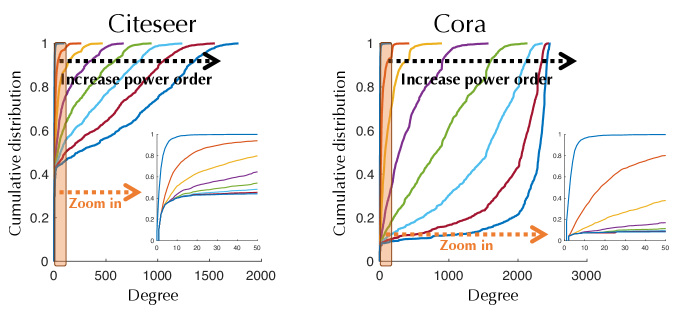
Figure 9: Degree distribution in the original graph and the powered graphs for Citeseer and Cora. The graph becomes more homogeneous and high degree nodes become more prevalent as we increase the powers.

Table 2: Citation datasets. Label rate denotes the fraction of training labels in each dataset.

Dataset	Nodes	Edges	Features	Classes	Label rates
Citeseer	3,327	4,732	3,703	6	0.036
Cora	2,708	5,429	1,433	7	0.052
Pubmed	19,717	44,338	500	3	0.003

Appendix D More experimental details and results

Experimental setup. We followed the setup of (Yang, Cohen, and Salakhutdinov 2016; Kipf and Welling 2017) for citation networks Citeseer, Cora and Pubmed. The statistics of datasets is in Table 2. Degree distribution in the original graph and the powered graphs for Citeseer and Cora is shown in Figure 9. We used the same dataset splits as in (Yang, Cohen, and Salakhutdinov 2016; Kipf and Welling 2017) with $20$ labels per class for training, $500$ labeled samples for hyper-parameter setting, and $1,000$ samples for testing. To facilitate comparison, we use the same hyper-parameters as Vanilla GCN (Kipf and Welling 2017), including number of layers ($2$), number of hidden units ($16$), dropout rates ($0.5$), weight decay ($5\times 10^{-4}$), and weight initialization following (Glorot and Bengio 2010) implemented in Tensorflow. The training process is terminated if validation accuracy does not improve for 40 consecutive steps. We note that the citation datasets are extremely sensitive to initializations; as such, we report the test accuracy for the top 50 runs out of 100 random initializations sorted by the validation accuracy. We used Adam (Kingma and Ba 2014) with a learning rate of 0.01 except for ${\bm{\theta}}$ (VPN), which was chosen to be $1\times 10^{-5}$ to stabilize training. For VPN, we consider two-step training process, i.e., we first employ graph sparsification on adjacency matrix $\bar{\bm{A}}^{[k]}$ based on $\bm{X}$ for the first-step training, then process second graph sparsification on adjacency matrix $\bar{\bm{A}}^{[k]}$ with respect to the feature embedding from hidden layer and fetch them back into model for second-step training with warm restart (continue training with the parameters from first-step). We set $\alpha_{k}$ to be 0.5 for the corresponding power order and 0 other wise in r-GCN.

To enhance robustness against evasion attack, we adaptively chose the threshold of graph sparsification. For each node, we consider all its neighbors within $r$ hops, where $r$ is the order of the powered graph. We order these neighbors based on their Euclidean distance to the current node in the feature space. We then set the threshold for this node such that only the first $s*d$ neighbors with the smallest distance are selected, where $s$ is the sparsification rate, and $d$ is the degree of the node in the original graph. If this node is a high-degree node (determined by if the degree is higher than the average degree by more than 2 standard deviations), we set $s=1$; otherwise, we set $s$ to be a small number slightly larger than 1. Nevertheless, we do not observe that the robustness performance is sensitive to this parameter. In addition, one can define their own distance function that better measures proximity between nodes, such as correlation distance or cosine distance. As a side remark, one can easily obtain $\bm{A}^{(r)}$ with $\text{1}[(\bm{I}+\bm{A})^{r}>0]$, and recursively calculate $\bm{A}^{[k]}$. The proposed methods have similar computational complexity as vanilla GCN as a result of sparsification.

It is true that the performance on clean datasets can be better with many simpler tricks, due to the fast development of this society and the simplicity of these citation datasets. However, we aim to demonstrate that both models we proposed can remarkably enhance the robustness of GNNs on perturbed graphs, while not losing the performance on clean ones, which should be highlighted as our main contribution.

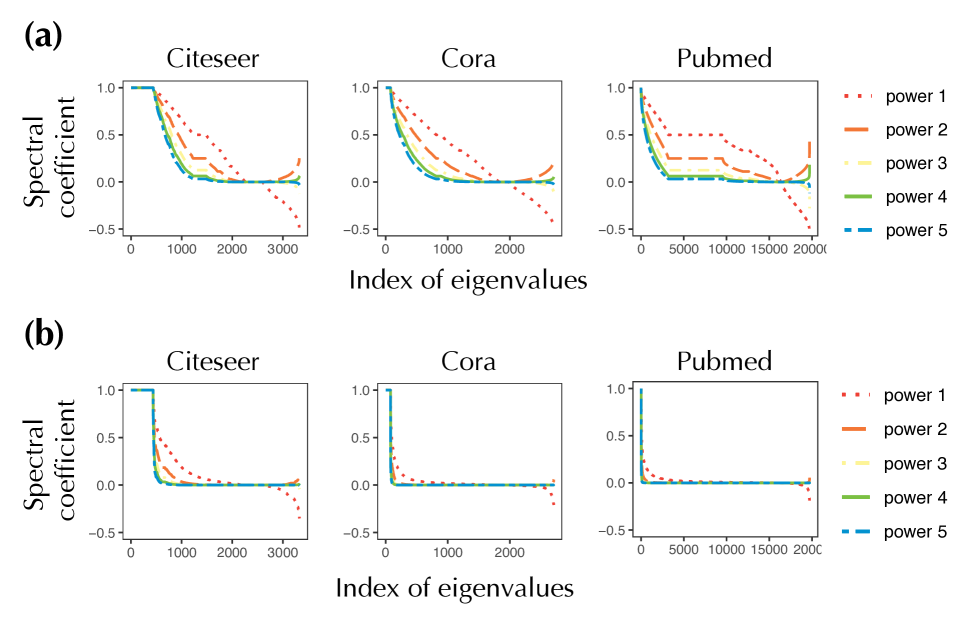
Figure 10: Eigenspectrum of (a) the adjacency matrix and (b) VPN raised to different powers. The convolution operator becomes similar to low-pass filters as we increase powers. The eigenspectrum of VPN also has sharper edges than the original adjacency matrix.

Revisiting SBM. To obtain networks with different SNRs (0.58, 0.68, 0.79, 0.85, 0.91), we set the intra-degree average $a_{\text{intra}}=2.1$ and inter-degree average $a_{\text{inter}}$ to be 0.4, 0.3, 0.2, 0.15, 0.1 respectively. We generate 10 networks for each SNR. One of the networks with SNR of 0.91 is analyzed in Figure 11 for different convolution operators. As predicted by Theorem 3, the proposed operators have nontrivial spectral gap. This is not enjoyed by other operators, so it is a quite unique property. Furthermore, our learned operator w/ or w/o normalization obtained 81% accuracy based on the second eigenvector, whereas adjacency matrix catches “high-degree nodes” and normalized (or powered) Laplacians catch “tails”, with spectral clustering accuracy of only 51%.

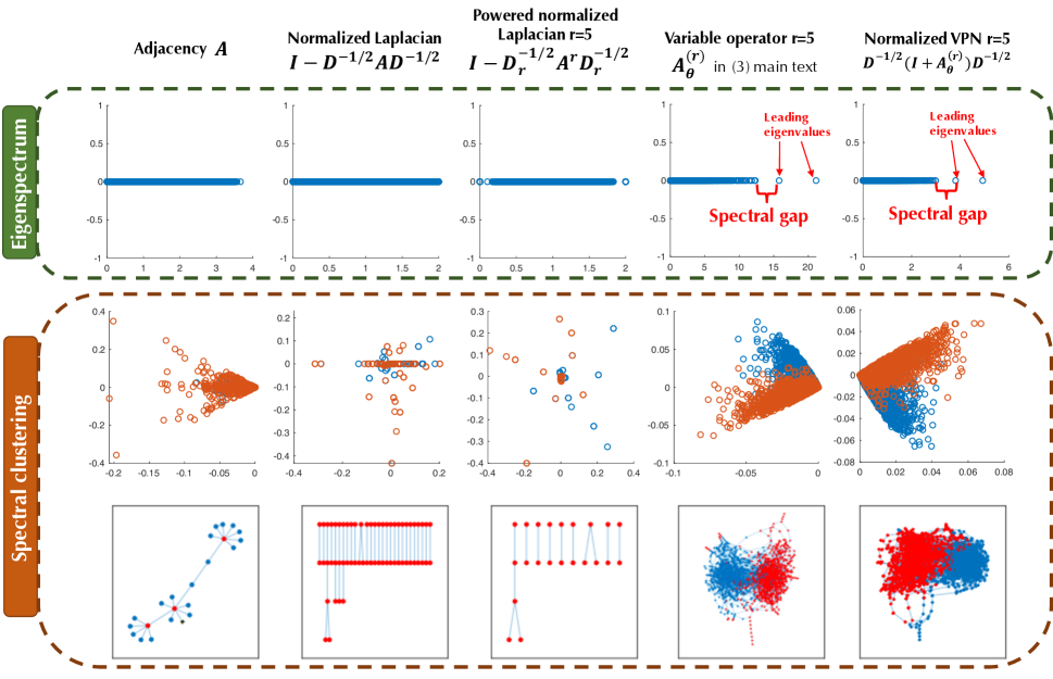
Figure 11: Illustration of operators for SBM, showing (top to bottom) the eigenspectrum, plots of the first 2 leading eigenvectors, and the detected clusters. We consider (from left to right) the adjacency matrix $\bm{A}$, normalized Laplacian $\bm{I}-\bm{D}^{-1/2}\bm{A}\bm{D}^{-1/2}$, powered normalized Laplacian $\bm{I}-\bm{D}_{r}^{-1/2}\bm{A}^{r}\bm{D}_{r}^{-1/2}$ ($\bm{D}_{r}$ is the degree matrix of $\bm{A}^{r}$), VPN $\bm{A}_{{\bm{\theta}}}^{(r)}$ with order 5 ($\theta_{k}$ is 1 when $k=1$ and 0.1 otherwise), and the normalized version $\bm{D}^{-1/2}(\bm{I}+\bm{A}_{{\bm{\theta}}}^{(r)})\bm{D}^{-1/2}$.

Visualization of network embeddings. We used t-SNE (Maaten and Hinton 2008) to visualize the network embeddings learned by r-GCN (Figure 12) and VPN (Figure 13) for Citeseer, Cora and Pubmed. As can be seen, with very limited labels, the proposed methods can learn an effective embedding of the nodes.

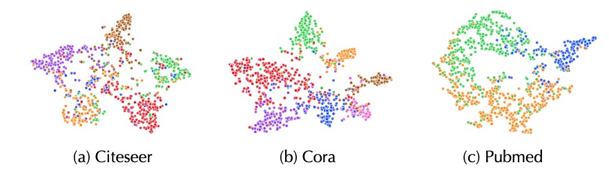
Figure 12: t-SNE visualization of network embeddings learned by r-GCN.

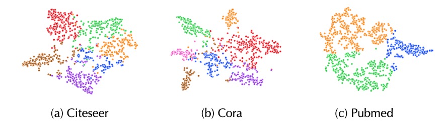
Figure 13: t-SNE visualization of network embeddings learned by VPN.

Evasion experiment. Five representative global adversarial attack methods are considered as comparisons:

• DICE (Zügner and Günnemann 2019) (remove internally, insert externally): it randomly disconnects nodes from the same class and connects nodes from different classes.

• $\mathcal{A}_{abr}$ and $\mathcal{A}_{DW_{3}}$ (Bojchevski and Günnemann 2019): both attack methods are matrix perturbation theory based. $\mathcal{A}_{DW_{3}}$ is the closed-form attack for edge deletion and $\mathcal{A}_{abr}$ is the add-by-remove strategy based method for edge insertion.

• Meta-Train and Meta-Self (Zügner and Günnemann 2019): both attack approaches are meta learning based. The meta-gradient approach with self-training is denoted as Meta-Self and the variant without self-training is denoted as Meta-Train. Note that both attack methods result in OOM (out of memory) on Pubmed, we choose to report the performance against them only on Citeseer and Cora.

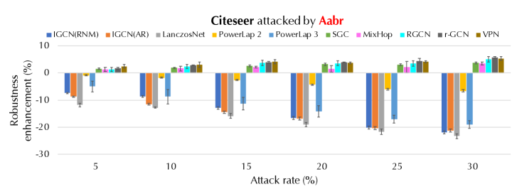
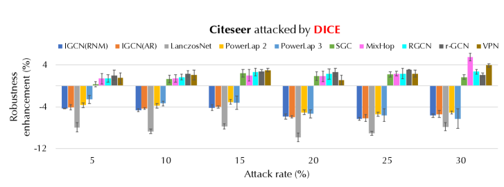
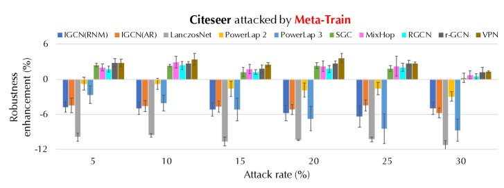
Figure 14: Illustration of evasion attack performance in terms of robustness enhancement on different attack methods (from top to bottom) for Citeseer: $\mathcal{A}_{abr}$ (Bojchevski and Günnemann 2019), DICE (Zügner and Günnemann 2019), Meta-Self and Meta-Train (Zügner and Günnemann 2019). Evaluated methods include IGCN (Li et al. 2019), LanczosNet (Liao et al. 2019), SGC (Wu et al. 2019), MixHop (Abu-El-Haija et al. 2019) and RGCN (Zhu et al. 2019). PowerLap 2 and 3 are methods that replace the adjacency matrix in GCN by its powered versions with orders 2 and 3, respectively. Positive values indicate improvement of robustness compared to vanilla GCN and negative ones indicate deterioration.

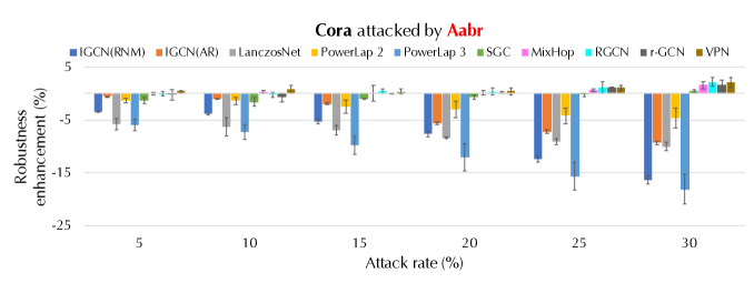
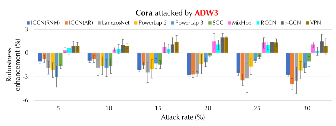
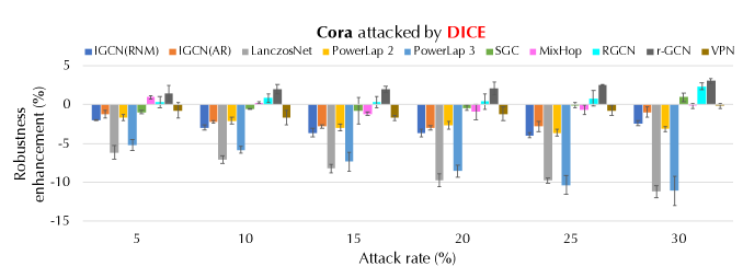
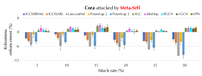
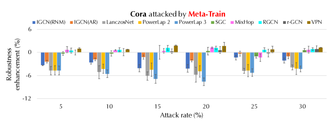
Figure 15: Illustration of evasion attack performance in terms of robustness enhancement on different attack methods for Cora.

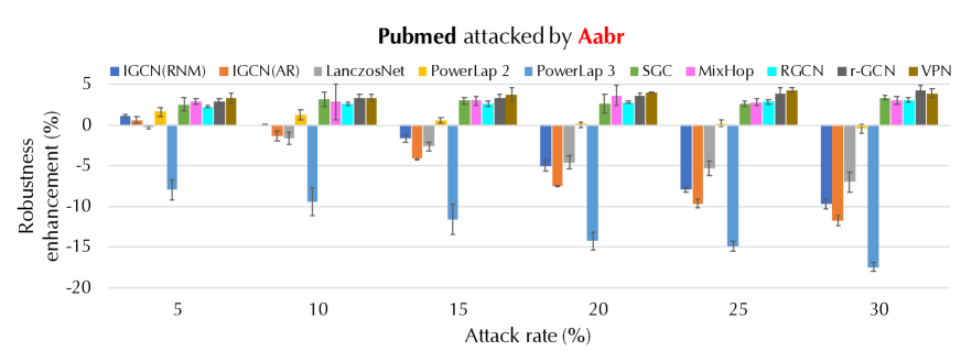
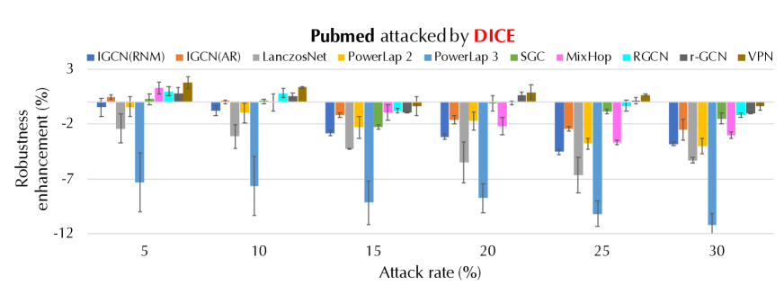
Figure 16: Illustration of evasion attack performance in terms of robustness enhancement on different attack methods for Pubmed.

We provide the post-evasion accuracy in Table 3 and Table 4 and robustness enhancement in Figure 14, Figure 15 and Figure 16 for Citeseer, Cora, and Pubmed. Results are obtained with 20 random initializations on a given attacked network.

Table 3: Summary of evasion attack performance on DICE, $\mathcal{A}_{abr}$ and $\mathcal{A}_{DW_{3}}$ in terms of post-evasion accuracy (in percent). Best performance under each setting is in bold.

	Attack Method	DICE
		Model
	Attack Rate (%)	GCN	IGCN(RNM)	IGCN(AR)	LanczosNet	RGCN	PowerLap 2	PowerLap 3	SGC	MixHop	r-GCN	VPN
Citeseer	5	$68.5\pm 0.7$	$64.1\pm 0.0$	$64.4\pm 0.5$	$60.6\pm 0.9$	$69.9\pm 0.7$	$64.8\pm 0.4$	$65.9\pm 0.7$	$68.8\pm 0.5$	$69.9\pm 1.0$	$70.5\pm 1.0$	$70.0\pm 1.0$
	10	$66.3\pm 0.1$	$61.6\pm 0.3$	$61.9\pm 0.2$	$57.6\pm 0.4$	$67.9\pm 0.5$	$62.5\pm 0.4$	$62.9\pm 0.4$	$67.5\pm 0.7$	$67.7\pm 0.7$	$68.6\pm 0.6$	$68.3\pm 0.9$
	15	$63.4\pm 0.2$	$59.3\pm 0.5$	$59.4\pm 0.2$	$55.7\pm 0.5$	$66.0\pm 0.7$	$60.4\pm 0.4$	$60.2\pm 1.2$	$65.8\pm 0.7$	$65.4\pm 1.1$	$66.2\pm 0.4$	$66.4\pm 0.3$
	20	$62.8\pm 0.4$	$56.9\pm 0.5$	$56.9\pm 0.2$	$53.0\pm 0.8$	$65.0\pm 1.0$	$57.8\pm 0.5$	$57.5\pm 0.7$	$64.7\pm 0.8$	$64.6\pm 1.0$	$65.4\pm 0.8$	$63.9\pm 0.9$
	25	$60.9\pm 0.6$	$54.6\pm 0.3$	$54.7\pm 0.7$	$51.8\pm 0.4$	$63.2\pm 1.0$	$55.5\pm 0.4$	$55.3\pm 1.2$	$63.1\pm 0.5$	$63.2\pm 0.4$	$63.9\pm 0.0$	$63.2\pm 0.6$
	30	$57.5\pm 1.1$	$51.9\pm 0.3$	$52.1\pm 0.7$	$49.7\pm 0.8$	$60.2\pm 0.5$	$52.4\pm 0.3$	$51.3\pm 1.9$	$59.2\pm 0.4$	$63.0\pm 0.7$	$59.6\pm 0.4$	$61.4\pm 0.4$
	Attack Rate (%)	GCN	IGCN(RNM)	IGCN(AR)	LanczosNet	RGCN	PowerLap 2	PowerLap 3	SGC	MixHop	r-GCN	VPN
Cora	5	$79.2\pm 0.3$	$77.2\pm 0.9$	$78.0\pm 0.3$	$73.0\pm 0.9$	$79.5\pm 0.4$	$77.5\pm 1.1$	$74.0\pm 0.5$	$78.2\pm 0.2$	$80.1\pm 0.2$	$80.6\pm 0.8$	$78.4\pm 0.2$
	10	$76.7\pm 0.7$	$73.7\pm 0.2$	$74.5\pm 0.7$	$69.6\pm 1.5$	$77.5\pm 0.5$	$74.6\pm 0.8$	$70.9\pm 0.5$	$76.1\pm 0.1$	$76.9\pm 0.1$	$78.6\pm 0.8$	$75.0\pm 0.3$
	15	$74.3\pm 0.2$	$70.7\pm 0.1$	$71.5\pm 1.2$	$66.1\pm 0.0$	$74.6\pm 0.2$	$71.4\pm 1.1$	$67.0\pm 0.6$	$73.5\pm 1.7$	$73.1\pm 0.2$	$76.3\pm 0.8$	$72.6\pm 0.3$
	20	$72.5\pm 0.6$	$68.9\pm 0.2$	$69.5\pm 0.6$	$62.8\pm 0.7$	$72.9\pm 0.2$	$69.9\pm 0.7$	$64.0\pm 0.3$	$72.1\pm 0.3$	$71.6\pm 1.0$	$74.6\pm 0.8$	$71.3\pm 0.3$
	25	$70.2\pm 0.9$	$66.2\pm 0.5$	$67.4\pm 0.9$	$60.4\pm 1.3$	$70.9\pm 0.4$	$66.6\pm 1.1$	$59.8\pm 0.7$	$70.1\pm 0.3$	$69.5\pm 0.6$	$72.7\pm 0.9$	$69.4\pm 0.3$
	30	$69.9\pm 0.4$	$67.5\pm 0.8$	$68.9\pm 1.4$	$58.7\pm 1.1$	$72.2\pm 0.6$	$66.7\pm 0.8$	$58.8\pm 0.8$	$70.8\pm 0.6$	$69.7\pm 0.3$	$72.9\pm 0.8$	$69.7\pm 0.5$
	Attack Rate (%)	GCN	IGCN(RNM)	IGCN(AR)	LanczosNet	RGCN	PowerLap 2	PowerLap 3	SGC	MixHop	r-GCN	VPN
Pubmed	5	$75.3\pm 0.4$	$74.8\pm 0.8$	$75.8\pm 0.2$	$72.9\pm 1.3$	$76.3\pm 0.4$	$74.9\pm 0.9$	$68.0\pm 2.7$	$75.6\pm 0.5$	$76.6\pm 0.5$	$76.1\pm 0.5$	$77.1\pm 0.6$
	10	$73.0\pm 0.5$	$72.3\pm 0.5$	$73.0\pm 0.2$	$69.9\pm 1.0$	$73.9\pm 0.4$	$72.1\pm 0.9$	$65.4\pm 2.7$	$73.1\pm 0.2$	$73.0\pm 0.8$	$73.6\pm 0.3$	$74.4\pm 0.1$
	15	$71.6\pm 0.1$	$68.8\pm 0.2$	$70.4\pm 0.2$	$67.4\pm 0.1$	$70.9\pm 0.2$	$69.3\pm 1.0$	$62.5\pm 2.0$	$79.4\pm 0.2$	$70.7\pm 0.7$	$70.7\pm 0.1$	$71.3\pm 0.9$
	20	$69.2\pm 0.6$	$66.1\pm 0.2$	$67.6\pm 0.4$	$63.7\pm 1.8$	$69.2\pm 0.2$	$67.5\pm 0.8$	$60.5\pm 1.3$	$69.1\pm 0.7$	$67.0\pm 0.8$	$69.8\pm 0.3$	$70.1\pm 0.7$
	25	$68.2\pm 0.6$	$63.6\pm 0.3$	$65.7\pm 0.2$	$61.5\pm 1.6$	$67.8\pm 0.5$	$64.4\pm 0.5$	$58.0\pm 1.2$	$67.3\pm 0.2$	$64.5\pm 0.2$	$68.3\pm 0.3$	$68.8\pm 0.1$
	30	$57.5\pm 0.9$	$63.7\pm 0.2$	$65.0\pm 1.0$	$62.2\pm 0.3$	$66.3\pm 0.2$	$63.5\pm 0.7$	$56.3\pm 1.0$	$66.0\pm 0.5$	$64.5\pm 0.3$	$66.5\pm 0.1$	$67.1\pm 0.3$
	Attack Method	$\mathcal{A}_{abr}$
		Model
	Attack Rate (%)	GCN	IGCN(RNM)	IGCN(AR)	LanczosNet	RGCN	PowerLap 2	PowerLap 3	SGC	MixHop	r-GCN	VPN
Citeseer	5	$69.2\pm 0.2$	$61.7\pm 0.1$	$60.4\pm 0.1$	$57.3\pm 0.7$	$70.4\pm 0.8$	$68.3\pm 0.2$	$64.1\pm 2.0$	$70.7\pm 0.2$	$70.4\pm 0.8$	$70.8\pm 0.5$	$71.6\pm 0.6$
	10	$67.8\pm 0.3$	$59.1\pm 0.3$	$56.3\pm 0.3$	$55.0\pm 0.2$	$70.2\pm 0.8$	$66.0\pm 0.2$	$59.0\pm 2.7$	$69.6\pm 0.3$	$69.4\pm 0.9$	$70.6\pm 0.0$	$70.8\pm 1.0$
	15	$66.6\pm 0.4$	$53.6\pm 0.4$	$52.1\pm 0.4$	$50.7\pm 0.9$	$70.2\pm 1.0$	$63.9\pm 0.2$	$55.3\pm 2.3$	$69.1\pm 0.3$	$68.7\pm 0.4$	$70.4\pm 0.4$	$70.6\pm 0.7$
	20	$66.4\pm 0.5$	$49.7\pm 0.5$	$49.5\pm 0.5$	$47.4\pm 0.8$	$69.9\pm 0.8$	$62.0\pm 0.3$	$52.2\pm 2.2$	$69.5\pm 0.5$	$67.9\pm 1.2$	$70.3\pm 0.2$	$70.1\pm 0.3$
	25	$65.6\pm 0.5$	$45.4\pm 0.6$	$45.3\pm 0.6$	$44.0\pm 1.0$	$69.1\pm 1.0$	$59.5\pm 0.3$	$48.6\pm 1.5$	$68.6\pm 0.4$	$67.7\pm 2.1$	$70.0\pm 0.9$	$69.7\pm 0.4$
	30	$63.8\pm 0.5$	$41.9\pm 0.6$	$42.6\pm 0.6$	$40.5\pm 0.9$	$68.7\pm 1.0$	$57.2\pm 0.4$	$44.8\pm 1.4$	$67.4\pm 0.3$	$67.3\pm 0.5$	$69.5\pm 0.4$	$69.1\pm 0.6$
	Attack Rate (%)	GCN	IGCN(RNM)	IGCN(AR)	LanczosNet	RGCN	PowerLap 2	PowerLap 3	SGC	MixHop	r-GCN	VPN
Cora	5	$81.1\pm 0.1$	$77.6\pm 0.1$	$80.5\pm 0.1$	$75.3\pm 1.0$	$81.0\pm 0.4$	$79.8\pm 0.4$	$75.2\pm 1.1$	$79.7\pm 0.6$	$81.1\pm 0.3$	$80.9\pm 0.9$	$81.5\pm 0.2$
	10	$80.3\pm 0.1$	$76.4\pm 0.2$	$79.3\pm 0.1$	$74.0\pm 1.7$	$80.0\pm 0.6$	$78.9\pm 0.7$	$73.0\pm 1.5$	$78.7\pm 0.8$	$80.6\pm 0.3$	$79.6\pm 0.8$	$81.1\pm 0.8$
	15	$79.7\pm 0.2$	$74.3\pm 0.4$	$77.7\pm 0.2$	$72.7\pm 1.0$	$80.1\pm 0.4$	$77.1\pm 1.2$	$69.9\pm 1.7$	$78.6\pm 0.1$	$79.7\pm 1.5$	$79.7\pm 0.1$	$80.0\pm 0.5$
	20	$78.9\pm 0.2$	$71.2\pm 0.5$	$73.2\pm 0.2$	$70.5\pm 0.2$	$79.2\pm 0.7$	$75.9\pm 1.6$	$66.8\pm 2.5$	$78.2\pm 0.4$	$79.0\pm 0.4$	$79.1\pm 0.2$	$79.3\pm 0.6$
	25	$77.4\pm 0.3$	$64.9\pm 0.6$	$70.1\pm 0.3$	$68.2\pm 0.6$	$78.5\pm 1.1$	$73.2\pm 1.4$	$61.7\pm 2.6$	$77.1\pm 0.3$	$78.0\pm 0.3$	$78.5\pm 0.1$	$78.4\pm 0.6$
	30	$75.6\pm 0.6$	$59.2\pm 0.7$	$66.2\pm 0.4$	$65.5\pm 0.8$	$77.7\pm 0.8$	$71.0\pm 1.9$	$57.4\pm 2.8$	$76.0\pm 0.3$	$77.1\pm 0.6$	$77.3\pm 0.8$	$77.6\pm 1.0$
	Attack Rate (%)	GCN	IGCN(RNM)	IGCN(AR)	LanczosNet	RGCN	PowerLap 2	PowerLap 3	SGC	MixHop	r-GCN	VPN
Pubmed	5	$75.3\pm 0.8$	$76.4\pm 0.2$	$75.9\pm 0.4$	$75.0\pm 0.2$	$77.6\pm 0.1$	$76.9\pm 0.5$	$67.3\pm 1.2$	$77.8\pm 0.8$	$78.2\pm 0.3$	$78.2\pm 0.3$	$78.6\pm 0.6$
	10	$74.3\pm 0.5$	$74.3\pm 0.1$	$73.0\pm 0.6$	$72.7\pm 0.8$	$77.0\pm 0.1$	$75.6\pm 0.6$	$64.9\pm 1.7$	$77.5\pm 0.9$	$77.2\pm 2.2$	$77.7\pm 0.5$	$77.7\pm 0.4$
	15	$73.5\pm 0.7$	$71.9\pm 0.4$	$69.4\pm 0.0$	$70.9\pm 0.6$	$76.1\pm 0.3$	$74.1\pm 0.3$	$61.9\pm 1.8$	$76.5\pm 0.4$	$76.5\pm 0.5$	$76.9\pm 0.4$	$77.3\pm 0.8$
	20	$73.7\pm 0.1$	$68.7\pm 0.7$	$66.2\pm 0.0$	$69.1\pm 0.8$	$76.5\pm 0.1$	$73.7\pm 0.3$	$59.4\pm 1.1$	$76.3\pm 1.1$	$77.3\pm 1.2$	$77.3\pm 0.4$	$77.7\pm 0.1$
	25	$72.9\pm 0.1$	$64.9\pm 0.2$	$63.2\pm 0.5$	$67.6\pm 0.9$	$75.8\pm 0.3$	$73.1\pm 0.5$	$58.0\pm 0.6$	$75.5\pm 0.4$	$75.7\pm 0.4$	$76.7\pm 0.7$	$77.2\pm 0.3$
	30	$72.8\pm 0.9$	$63.1\pm 0.6$	$61.1\pm 0.6$	$65.8\pm 1.2$	$75.9\pm 0.2$	$72.4\pm 0.6$	$55.4\pm 0.6$	$76.2\pm 0.3$	$75.9\pm 0.5$	$77.2\pm 0.6$	$76.7\pm 0.5$
	Attack Method	$\mathcal{A}_{DW_{3}}$
		Model
	Attack Rate (%)	GCN	IGCN(RNM)	IGCN(AR)	LanczosNet	RGCN	PowerLap 2	PowerLap 3	SGC	MixHop	r-GCN	VPN
Citeseer	5	$68.8\pm 0.1$	$63.5\pm 0.4$	$65.1\pm 0.2$	$60.0\pm 0.5$	$70.3\pm 0.6$	$69.2\pm 1.0$	$70.0\pm 0.8$	$70.5\pm 0.5$	$70.4\pm 1.0$	$71.8\pm 0.3$	$70.6\pm 0.6$
	10	$68.4\pm 0.2$	$63.1\pm 0.6$	$63.6\pm 0.5$	$59.6\pm 0.6$	$70.1\pm 0.6$	$69.3\pm 1.1$	$69.6\pm 0.6$	$70.1\pm 0.8$	$69.4\pm 0.4$	$71.2\pm 0.7$	$70.2\pm 0.7$
	15	$68.9\pm 0.1$	$62.9\pm 0.7$	$63.2\pm 0.8$	$59.5\pm 0.9$	$70.3\pm 0.4$	$69.5\pm 1.1$	$69.8\pm 0.7$	$70.6\pm 0.8$	$68.7\pm 1.4$	$71.2\pm 0.1$	$70.6\pm 0.4$
	20	$68.8\pm 0.5$	$63.5\pm 0.8$	$63.4\pm 0.7$	$59.1\pm 0.8$	$69.8\pm 0.4$	$69.4\pm 1.0$	$69.5\pm 0.7$	$70.3\pm 0.2$	$67.9\pm 1.4$	$71.1\pm 0.2$	$70.4\pm 0.7$
	25	$68.8\pm 0.4$	$63.6\pm 0.7$	$63.8\pm 0.6$	$59.3\pm 0.4$	$69.9\pm 0.5$	$69.2\pm 0.9$	$69.3\pm 0.9$	$70.2\pm 0.5$	$67.7\pm 0.8$	$71.2\pm 0.1$	$70.1\pm 0.2$
	30	$68.8\pm 0.4$	$63.6\pm 0.7$	$63.8\pm 0.6$	$59.3\pm 0.1$	$69.9\pm 0.5$	$69.2\pm 0.9$	$69.3\pm 0.9$	$70.2\pm 0.7$	$67.3\pm 0.1$	$71.2\pm 0.0$	$70.1\pm 0.9$
	Attack Rate (%)	GCN	IGCN(RNM)	IGCN(AR)	LanczosNet	RGCN	PowerLap 2	PowerLap 3	SGC	MixHop	r-GCN	VPN
Cora	5	$80.0\pm 0.7$	$78.9\pm 0.2$	$79.2\pm 0.4$	$78.1\pm 0.8$	$80.5\pm 0.9$	$77.8\pm 0.9$	$77.0\pm 1.4$	$78.3\pm 0.3$	$80.3\pm 0.3$	$80.8\pm 0.7$	$80.8\pm 0.5$
	10	$79.7\pm 0.9$	$78.7\pm 0.2$	$78.9\pm 0.4$	$77.8\pm 1.0$	$80.1\pm 0.6$	$78.1\pm 1.1$	$77.8\pm 1.1$	$78.0\pm 0.9$	$80.1\pm 0.2$	$80.7\pm 0.8$	$80.5\pm 0.3$
	15	$79.3\pm 0.7$	$77.1\pm 0.2$	$77.7\pm 0.4$	$76.8\pm 1.2$	$79.7\pm 0.5$	$77.3\pm 1.2$	$77.9\pm 0.6$	$77.8\pm 0.5$	$80.0\pm 0.7$	$80.3\pm 0.9$	$80.6\pm 0.9$
	20	$78.3\pm 1.0$	$75.5\pm 0.2$	$75.6\pm 0.3$	$75.7\pm 0.3$	$79.3\pm 0.6$	$76.9\pm 1.2$	$77.1\pm 0.5$	$78.0\pm 0.2$	$79.8\pm 1.0$	$80.3\pm 0.5$	$80.3\pm 0.2$
	25	$77.8\pm 0.6$	$75.3\pm 0.3$	$74.4\pm 0.7$	$74.6\pm 1.8$	$78.7\pm 0.5$	$76.1\pm 1.0$	$76.8\pm 0.2$	$77.3\pm 0.2$	$79.1\pm 0.7$	$79.2\pm 0.0$	$79.1\pm 0.5$
	30	$77.8\pm 0.8$	$75.0\pm 0.2$	$73.8\pm 0.7$	$74.3\pm 1.7$	$78.0\pm 0.5$	$75.6\pm 1.1$	$75.9\pm 0.6$	$76.7\pm 0.6$	$78.8\pm 0.4$	$79.3\pm 0.9$	$78.6\pm 1.0$
	Attack Rate (%)	GCN	IGCN(RNM)	IGCN(AR)	LanczosNet	RGCN	PowerLap 2	PowerLap 3	SGC	MixHop	r-GCN	VPN
Pubmed	5	$78.3\pm 0.5$	$79.3\pm 0.4$	$79.2\pm 0.1$	$76.5\pm 1.8$	$77.8\pm 0.1$	$74.8\pm 1.7$	$76.5\pm 0.5$	$78.0\pm 0.4$	$78.2\pm 0.5$	$78.1\pm 0.7$	$79.0\pm 1.0$
	10	$77.8\pm 0.2$	$78.6\pm 0.2$	$78.6\pm 0.7$	$75.3\pm 1.0$	$77.9\pm 0.3$	$74.7\pm 1.9$	$77.4\pm 0.4$	$77.8\pm 1.0$	$78.0\pm 0.7$	$77.9\pm 0.9$	$78.6\pm 0.1$
	15	$77.4\pm 0.4$	$77.0\pm 0.4$	$77.2\pm 0.3$	$74.7\pm 0.3$	$77.5\pm 0.3$	$74.2\pm 1.5$	$76.9\pm 0.4$	$77.3\pm 0.4$	$77.3\pm 0.8$	$77.8\pm 0.3$	$78.3\pm 0.2$
	20	$77.4\pm 0.4$	$75.8\pm 0.3$	$76.3\pm 0.4$	$73.5\pm 1.8$	$77.8\pm 0.4$	$73.8\pm 1.0$	$76.3\pm 0.4$	$77.3\pm 1.2$	$77.1\pm 0.3$	$77.6\pm 1.0$	$78.3\pm 0.4$
	25	$77.2\pm 0.5$	$75.2\pm 0.1$	$75.9\pm 0.4$	$73.7\pm 1.1$	$77.6\pm 0.3$	$73.7\pm 1.1$	$75.6\pm 0.7$	$77.1\pm 0.2$	$77.0\pm 0.3$	$78.1\pm 0.8$	$78.2\pm 0.2$
	30	$77.1\pm 0.2$	$74.5\pm 0.3$	$74.6\pm 0.3$	$73.4\pm 0.3$	$77.0\pm 0.2$	$72.9\pm 1.4$	$74.6\pm 0.4$	$77.1\pm 0.3$	$77.2\pm 0.8$	$77.6\pm 0.3$	$77.7\pm 0.9$

Table 4: Summary of evasion attack performance on Meta-Train and Meta-Self in terms of post-evasion accuracy (in percent). OOM (out of memory) for both methods on Pubmed.

	Attack Method	Meta-Train
		Model
	Attack Rate (%)	GCN	IGCN(RNM)	IGCN(AR)	LanczosNet	RGCN	PowerLap 2	PowerLap 3	SGC	MixHop	r-GCN	VPN
Citeseer	5	$67.6\pm 0.3$	$62.8\pm 0.8$	$63.1\pm 1.2$	$57.7\pm 0.7$	$69.3\pm 0.5$	$66.8\pm 1.1$	$64.9\pm 1.5$	$70.0\pm 0.3$	$69.6\pm 0.6$	$70.4\pm 0.7$	$70.4\pm 0.6$
	10	$66.0\pm 1.0$	$61.0\pm 1.1$	$61.4\pm 1.0$	$56.4\pm 0.3$	$68.3\pm 0.7$	$65.2\pm 0.9$	$61.9\pm 1.4$	$68.3\pm 0.2$	$68.9\pm 1.0$	$68.7\pm 0.4$	$69.4\pm 1.0$
	15	$66.1\pm 0.6$	$60.9\pm 1.1$	$61.4\pm 1.0$	$55.4\pm 0.8$	$67.3\pm 0.4$	$64.5\pm 1.3$	$60.9\pm 1.9$	$67.3\pm 0.8$	$67.8\pm 0.8$	$67.9\pm 0.6$	$68.6\pm 0.3$
	20	$64.9\pm 0.9$	$59.1\pm 1.4$	$59.7\pm 0.8$	$54.5\pm 0.1$	$66.6\pm 0.6$	$63.0\pm 1.2$	$58.2\pm 2.1$	$67.2\pm 0.5$	$67.1\pm 0.9$	$67.6\pm 0.4$	$68.5\pm 0.8$
	25	$64.3\pm 0.7$	$57.9\pm 1.8$	$59.8\pm 1.0$	$54.0\pm 0.4$	$66.3\pm 0.7$	$62.7\pm 1.1$	$55.8\pm 2.6$	$66.1\pm 0.5$	$66.5\pm 1.7$	$67.0\pm 0.5$	$67.0\pm 0.2$
	30	$64.8\pm 1.1$	$59.8\pm 1.0$	$59.0\pm 0.8$	$53.5\pm 0.8$	$65.2\pm 0.4$	$61.8\pm 0.8$	$56.1\pm 1.9$	$65.0\pm 0.8$	$65.5\pm 0.7$	$66.0\pm 0.8$	$66.1\pm 0.1$
	Attack Rate (%)	GCN	IGCN(RNM)	IGCN(AR)	LanczosNet	RGCN	PowerLap 2	PowerLap 3	SGC	MixHop	r-GCN	VPN
Cora	5	$79.8\pm 0.9$	$76.5\pm 0.1$	$77.4\pm 0.3$	$75.1\pm 1.1$	$80.2\pm 0.7$	$75.2\pm 1.2$	$75.1\pm 1.1$	$79.5\pm 0.5$	$80.5\pm 0.8$	$79.8\pm 0.6$	$80.8\pm 0.2$
	10	$78.4\pm 0.7$	$75.8\pm 0.4$	$76.6\pm 0.3$	$73.3\pm 1.7$	$79.0\pm 0.5$	$74.2\pm 1.2$	$72.9\pm 1.0$	$78.1\pm 0.7$	$79.0\pm 0.1$	$78.5\pm 0.9$	$79.2\pm 0.1$
	15	$77.9\pm 0.6$	$73.8\pm 0.9$	$76.7\pm 0.6$	$71.8\pm 1.1$	$79.0\pm 0.7$	$73.4\pm 1.7$	$71.0\pm 1.1$	$77.9\pm 1.8$	$78.3\pm 0.6$	$78.2\pm 0.6$	$79.7\pm 0.1$
	20	$76.0\pm 1.4$	$71.8\pm 1.0$	$73.8\pm 0.3$	$70.2\pm 1.9$	$77.1\pm 0.5$	$71.0\pm 1.5$	$68.4\pm 1.0$	$76.3\pm 1.0$	$77.2\pm 0.2$	$76.6\pm 0.9$	$77.6\pm 1.0$
	25	$79.1\pm 0.6$	$77.7\pm 0.6$	$78.7\pm 0.6$	$74.3\pm 0.7$	$79.7\pm 0.6$	$74.3\pm 1.6$	$73.8\pm 1.0$	$78.0\pm 0.4$	$77.7\pm 1.0$	$78.9\pm 1.0$	$79.8\pm 0.9$
	30	$77.7\pm 0.9$	$75.6\pm 0.7$	$76.7\pm 0.6$	$73.8\pm 0.7$	$78.6\pm 0.4$	$73.5\pm 1.6$	$73.4\pm 0.7$	$78.3\pm 0.4$	$78.4\pm 0.9$	$78.6\pm 0.9$	$79.0\pm 0.0$
	Attack Method	Meta-Self
		Model
	Attack Rate (%)	GCN	IGCN(RNM)	IGCN(AR)	LanczosNet	RGCN	PowerLap 2	PowerLap 3	SGC	MixHop	r-GCN	VPN
Citeseer	5	$66.2\pm 0.9$	$61.8\pm 0.1$	$60.9\pm 0.8$	$60.2\pm 0.2$	$69.1\pm 0.4$	$66.3\pm 0.9$	$66.0\pm 1.2$	$69.1\pm 0.3$	$69.6\pm 0.4$	$70.1\pm 0.7$	$69.1\pm 0.8$
	10	$64.7\pm 0.8$	$59.3\pm 0.4$	$59.1\pm 0.9$	$57.3\pm 0.1$	$67.3\pm 0.6$	$64.4\pm 0.8$	$62.5\pm 1.3$	$67.9\pm 0.7$	$67.1\pm 0.5$	$68.0\pm 0.0$	$68.2\pm 0.7$
	15	$64.0\pm 0.9$	$57.2\pm 0.3$	$58.1\pm 0.7$	$55.2\pm 0.2$	$65.9\pm 0.9$	$62.9\pm 1.7$	$60.6\pm 0.7$	$66.3\pm 0.9$	$66.2\pm 0.4$	$67.3\pm 0.9$	$66.2\pm 0.1$
	20	$62.4\pm 1.2$	$55.5\pm 0.2$	$56.8\pm 0.8$	$55.9\pm 0.4$	$65.3\pm 1.2$	$61.2\pm 1.5$	$58.6\pm 1.9$	$65.3\pm 1.0$	$64.9\pm 0.1$	$66.3\pm 0.4$	$65.6\pm 0.4$
	25	$62.7\pm 1.0$	$56.6\pm 0.7$	$58.4\pm 1.1$	$55.3\pm 0.3$	$65.1\pm 0.7$	$60.5\pm 1.6$	$57.6\pm 1.9$	$65.6\pm 0.8$	$65.0\pm 0.6$	$65.9\pm 0.5$	$65.5\pm 0.5$
	30	$61.1\pm 0.9$	$55.9\pm 0.5$	$56.4\pm 0.7$	$54.9\pm 0.1$	$64.7\pm 0.3$	$60.3\pm 1.5$	$57.5\pm 1.4$	$64.1\pm 0.8$	$64.5\pm 1.2$	$66.0\pm 1.0$	$64.5\pm 0.9$
	Attack Rate (%)	GCN	IGCN(RNM)	IGCN(AR)	LanczosNet	RGCN	PowerLap 2	PowerLap 3	SGC	MixHop	r-GCN	VPN
Cora	5	$78.7\pm 0.2$	$76.1\pm 0.3$	$75.0\pm 0.4$	$73.4\pm 0.5$	$79.6\pm 0.6$	$77.9\pm 1.4$	$74.7\pm 0.7$	$77.9\pm 0.6$	$79.0\pm 0.8$	$79.3\pm 0.8$	$79.1\pm 0.5$
	10	$76.8\pm 0.3$	$76.0\pm 0.5$	$74.3\pm 0.7$	$71.0\pm 1.8$	$78.4\pm 0.3$	$76.0\pm 0.9$	$72.6\pm 0.6$	$76.8\pm 0.2$	$77.2\pm 0.1$	$77.8\pm 0.9$	$78.0\pm 0.7$
	15	$75.3\pm 0.9$	$74.0\pm 0.5$	$72.1\pm 0.4$	$69.4\pm 0.0$	$77.1\pm 0.7$	$74.2\pm 1.4$	$69.5\pm 1.2$	$76.6\pm 0.4$	$77.0\pm 0.6$	$77.0\pm 0.7$	$77.5\pm 0.9$
	20	$75.8\pm 0.7$	$72.6\pm 0.7$	$71.1\pm 0.8$	$69.5\pm 1.4$	$76.3\pm 0.5$	$73.3\pm 1.2$	$70.4\pm 1.4$	$75.9\pm 0.3$	$76.3\pm 0.4$	$76.1\pm 0.9$	$76.4\pm 0.5$
	25	$77.5\pm 0.2$	$73.8\pm 0.2$	$73.4\pm 0.6$	$70.3\pm 0.2$	$78.4\pm 0.4$	$74.2\pm 1.0$	$70.9\pm 1.0$	$76.9\pm 0.3$	$77.6\pm 0.2$	$77.9\pm 0.2$	$77.8\pm 0.1$
	30	$76.7\pm 0.6$	$73.7\pm 0.6$	$72.2\pm 1.0$	$66.7\pm 0.0$	$78.4\pm 0.5$	$72.6\pm 1.2$	$67.0\pm 1.4$	$77.9\pm 0.2$	$78.0\pm 0.7$	$78.1\pm 0.5$	$78.5\pm 0.4$

Computational efficiency. The adjacency matrix could be much denser after being powered several times, which poses a general challenge for all high-order matrix-based approaches. To alleviate this issue, we employ a simple sparsification strategy as described in the main paper. To demonstrate the computational efficiency of the proposed method, we introduce a running time comparison experiment on the real world social network (Social circles: Facebook) (Leskovec and Mcauley 2012). This small dataset consists of “circles” (or “friends lists”) from Facebook and becomes very dense from first order ($4.71\%$) to second order ($92.12\%$), thus is suitable to be used for computational efficiency evaluation. The results are shown in Table 5. We can find that the running efficiency of the proposed method is compatible with baselines and the density does not affect the efficiency significantly when the dataset is not too large. Moreover, in this paper, our primary goal is to improve the robustness. We leave the solution to resolve the scalability issue as a future direction.

Table 5: Running time comparison on a social network dataset  (Leskovec and Mcauley 2012).

Methods	Vanilla GCN	PowerLaplacian	IGCN(RNM)	IGCN(AR)	LNet	RGCN	SGC	MixHop	r-GCN	VPN
Running Time (sec)	6.02	6.36	3.33	7.21	5.56	18.14	0.231	11.38	6.73	7.18

Appendix E More discussiones

Why second eigenvector fails? In the case of sparse graph (the expected degree is constant w.r.t. the size of the graph $n$), the largest eigenvalue of adjacency matrix $A$ is on the order of $\Theta(\sqrt{\frac{\log(n)}{\log\log(n)}})$ that corresponds to the high-degree nodes. To see this, the (squared) eigenvalue created by a node $v$ is $e_{v}^{\top}A^{2}e_{v}=\|Ae_{v}\|_{2}^{2}$, which is the degree of vertex $v$, where $e_{v}$ is a vector with only a one on the vertex $v$ and zero elsewhere. Then max of this term over all vertices is the maximum degree. Since the degree in the sparse case is roughly Poisson of a constant expectation, the maximum of $n$ weakly correlated Poisson r.v.s behaves like $\Theta({\frac{\log(n)}{\log\log(n)}})$, which can be arbitrarily large as the size $n$ grows. Therefore, without proper adjustments, the “useful” second eigenvalue is hiding in a bunch of outliers created by the high-degree nodes.

Can the limited spatial scope of graph Laplacian be alleviated by more layers? Naively adding more layers in GNNs will suffer from the ’over-smoothing’ problem. While constructing deep GNNs is a new trend but difficult to alleviate the ’over-smoothing’ problem while enjoying larger spatial scope[1,2], developing operators encounters the limited spatial scope of graph Laplacian is also very necessary as alternative approaches.

References

- Abbe et al. (2018) Abbe, E.; Boix, E.; Ralli, P.; and Sandon, C. 2018. Graph powering and spectral robustness. arXiv preprint arXiv:1809.04818 .
- Abu-El-Haija et al. (2018) Abu-El-Haija, S.; Kapoor, A.; Perozzi, B.; and Lee, J. 2018. N-GCN: Multi-scale graph convolution for semi-supervised node classification. arXiv preprint arXiv:1802.08888 .
- Abu-El-Haija et al. (2019) Abu-El-Haija, S.; Perozzi, B.; Kapoor, A.; Harutyunyan, H.; Alipourfard, N.; Lerman, K.; Steeg, G. V.; and Galstyan, A. 2019. MixHop: Higher-Order Graph Convolution Architectures via Sparsified Neighborhood Mixing. arXiv preprint arXiv:1905.00067 .
- Amini et al. (2013) Amini, A. A.; Chen, A.; Bickel, P. J.; Levina, E.; et al. 2013. Pseudo-likelihood methods for community detection in large sparse networks. The Annals of Statistics 41(4): 2097–2122.
- Atwood and Towsley (2016) Atwood, J.; and Towsley, D. 2016. Diffusion-convolutional neural networks. In NIPS 2016, 1993–2001.
- Balakrishnan et al. (2011) Balakrishnan, S.; Xu, M.; Krishnamurthy, A.; and Singh, A. 2011. Noise thresholds for spectral clustering. In NIPS 2011, 954–962.
- Bastings et al. (2017) Bastings, J.; Titov, I.; Aziz, W.; Marcheggiani, D.; and Sima’an, K. 2017. Graph convolutional encoders for syntax-aware neural machine translation. In EMNLP 2017, 1957–1967.
- Belkin and Niyogi (2002) Belkin, M.; and Niyogi, P. 2002. Laplacian eigenmaps and spectral techniques for embedding and clustering. In NIPS 2002, 585–591.
- Belkin, Niyogi, and Sindhwani (2006) Belkin, M.; Niyogi, P.; and Sindhwani, V. 2006. Manifold Regularization: A Geometric Framework for Learning from Labeled and Unlabeled Examples. Journal of Machine Learning Research 7: 2399–2434.
- Bojchevski and Günnemann (2019) Bojchevski, A.; and Günnemann, S. 2019. Adversarial Attacks on Node Embeddings via Graph Poisoning. In International Conference on Machine Learning, 695–704.
- Bordenave, Lelarge, and Massoulié (2015) Bordenave, C.; Lelarge, M.; and Massoulié, L. 2015. Non-backtracking spectrum of random graphs: community detection and non-regular ramanujan graphs. In FOCS 2015, 1347–1357. IEEE.
- Bruna et al. (2014) Bruna, J.; Zaremba, W.; Szlam, A.; and LeCun, Y. 2014. Spectral networks and locally connected networks on graphs. In ICLR 2014.
- Chang et al. (2020a) Chang, H.; Rong, Y.; Xu, T.; Huang, W.; Sojoudi, S.; Huang, J.; and Zhu, W. 2020a. Spectral Graph Attention Network with Fast Eigen-approximation. arXiv preprint arXiv:2003.07450 .
- Chang et al. (2021) Chang, H.; Rong, Y.; Xu, T.; Huang, W.; Zhang, H.; Cui, P.; Wang, X.; Zhu, W.; and Huang, J. 2021. Adversarial Attack Framework on Graph Embedding Models with Limited Knowledge. arXiv preprint arXiv:2105.12419 .
- Chang et al. (2020b) Chang, H.; Rong, Y.; Xu, T.; Huang, W.; Zhang, H.; Cui, P.; Zhu, W.; and Huang, J. 2020b. A restricted black-box adversarial framework towards attacking graph embedding models. In Proceedings of the AAAI Conference on Artificial Intelligence, volume 34, 3389–3396.
- Chaudhuri, Chung, and Tsiatas (2012) Chaudhuri, K.; Chung, F.; and Tsiatas, A. 2012. Spectral Clustering of Graphs with General Degrees in the Extended Planted Partition Model. Journal of Machine Learning Research 2012: 1–23.
- Chen et al. (2019) Chen, J.; Wu, Y.; Lin, X.; and Xuan, Q. 2019. Can Adversarial Network Attack be Defended? arXiv preprint arXiv:1903.05994 .
- Chung and Graham (1997) Chung, F. R.; and Graham, F. C. 1997. Spectral graph theory. 92. American Mathematical Soc.
- Coja-Oghlan (2010) Coja-Oghlan, A. 2010. Graph partitioning via adaptive spectral techniques. Combinatorics, Probability and Computing 19(2): 227–284.
- Dai et al. (2018) Dai, H.; Li, H.; Tian, T.; Huang, X.; Wang, L.; Zhu, J.; and Song, L. 2018. Adversarial Attack on Graph Structured Data. In International Conference on Machine Learning, 1123–1132.
- Davis and Kahan (1970) Davis, C.; and Kahan, W. M. 1970. The rotation of eigenvectors by a perturbation: III. SIAM Journal on Numerical Analysis 7(1): 1–46.
- Decelle et al. (2011) Decelle, A.; Krzakala, F.; Moore, C.; and Zdeborová, L. 2011. Asymptotic analysis of the stochastic block model for modular networks and its algorithmic applications. Physical Review E 84(6): 066106.
- Diakonikolas et al. (2019) Diakonikolas, I.; Kamath, G.; Kane, D.; Li, J.; Moitra, A.; and Stewart, A. 2019. Robust Estimators in High-Dimensions Without the Computational Intractability. SIAM Journal on Computing 48(2): 742–864.
- Feige and Ofek (2005) Feige, U.; and Ofek, E. 2005. Spectral techniques applied to sparse random graphs. Random Structures & Algorithms 27(2): 251–275.
- Fout et al. (2017) Fout, A.; Byrd, J.; Shariat, B.; and Ben-Hur, A. 2017. Protein interface prediction using graph convolutional networks. In NIPS 2017, 6530–6539.
- Friedman (2004) Friedman, J. 2004. A proof of Alon’s second eigenvalue conjecture and related problems. Mem. Amer. Math. Soc. (910).
- Glorot and Bengio (2010) Glorot, X.; and Bengio, Y. 2010. Understanding the difficulty of training deep feedforward neural networks. In AISTATS 2010, 249–256.
- Goodfellow, Shlens, and Szegedy (2015) Goodfellow, I. J.; Shlens, J.; and Szegedy, C. 2015. Explaining and harnessing adversarial examples. In ICLR 2015.
- Gu et al. (2020) Gu, F.; Chang, H.; Zhu, W.; Sojoudi, S.; and Ghaoui, L. E. 2020. Implicit graph neural networks. arXiv preprint arXiv:2009.06211 .
- Guan et al. (2021) Guan, C.; Zhang, Z.; Li, H.; Chang, H.; Zhang, Z.; Qin, Y.; Jiang, J.; Wang, X.; and Zhu, W. 2021. AutoGL: A Library for Automated Graph Learning. arXiv preprint arXiv:2104.04987 .
- Hamilton, Ying, and Leskovec (2017) Hamilton, W. L.; Ying, Z.; and Leskovec, J. 2017. Inductive Representation Learning on Large Graphs. NIPS 2017 1024–1034.
- Hammond, Vandergheynst, and Gribonval (2011) Hammond, D. K.; Vandergheynst, P.; and Gribonval, R. 2011. Wavelets on graphs via spectral graph theory. Applied and Computational Harmonic Analysis 30(2): 129–150.
- Henaff, Bruna, and LeCun (2015) Henaff, M.; Bruna, J.; and LeCun, Y. 2015. Deep convolutional networks on graph-structured data. arXiv preprint arXiv:1506.05163 .
- Holland, Laskey, and Leinhardt (1983) Holland, P. W.; Laskey, K. B.; and Leinhardt, S. 1983. Stochastic blockmodels: First steps. Social Networks 5(2): 109–137.
- Jacobsen, Smeulders, and Oyallon (2018) Jacobsen, J.-H.; Smeulders, A.; and Oyallon, E. 2018. i-RevNet: Deep Invertible Networks. In ICLR 2018.
- Joseph, Yu et al. (2016) Joseph, A.; Yu, B.; et al. 2016. Impact of regularization on spectral clustering. The Annals of Statistics 44(4): 1765–1791.
- Kaufmann, Bonald, and Lelarge (2016) Kaufmann, E.; Bonald, T.; and Lelarge, M. 2016. A spectral algorithm with additive clustering for the recovery of overlapping communities in networks. In ALT 2016, 355–370. Springer.
- Kearnes et al. (2016) Kearnes, S.; McCloskey, K.; Berndl, M.; Pande, V.; and Riley, P. 2016. Molecular graph convolutions: moving beyond fingerprints. Journal of computer-aided molecular design 30(8): 595–608.
- Kingma and Ba (2014) Kingma, D. P.; and Ba, J. 2014. Adam: A method for stochastic optimization. arXiv preprint arXiv:1412.6980 .
- Kipf and Welling (2017) Kipf, T. N.; and Welling, M. 2017. Semi-supervised classification with graph convolutional networks. In ICLR 2017.
- Le, Levina, and Vershynin (2015) Le, C. M.; Levina, E.; and Vershynin, R. 2015. Sparse random graphs: regularization and concentration of the laplacian. arXiv preprint arXiv:1502.03049 .
- Lee et al. (2018) Lee, J. B.; Rossi, R. A.; Kong, X.; Kim, S.; Koh, E.; and Rao, A. 2018. Higher-order graph convolutional networks. arXiv preprint arXiv:1809.07697 .
- Lee, Gharan, and Trevisan (2014) Lee, J. R.; Gharan, S. O.; and Trevisan, L. 2014. Multiway spectral partitioning and higher-order cheeger inequalities. Journal of the ACM 61(6): 37.
- Leskovec and Mcauley (2012) Leskovec, J.; and Mcauley, J. J. 2012. Learning to Discover Social Circles in Ego Networks. In Advances in Neural Information Processing Systems 25, 539–547.
- Li et al. (2019) Li, Q.; Wu, X.-M.; Liu, H.; Zhang, X.; and Guan, Z. 2019. Label efficient semi-supervised learning via graph filtering. In CVPR 2019, 9582–9591.
- Li et al. (2007) Li, Z.; Liu, J.; Chen, S.; and Tang, X. 2007. Noise robust spectral clustering. In ICCV 2007, 1–8.
- Liao et al. (2019) Liao, R.; Zhao, Z.; Urtasun, R.; and Zemel, R. S. 2019. LanczosNet: Multi-Scale Deep Graph Convolutional Networks. In ICLR 2019.
- Lu and Getoor (2003) Lu, Q.; and Getoor, L. 2003. Link-based classification. In ICML 2003, 496–503.
- Maaten and Hinton (2008) Maaten, L. v. d.; and Hinton, G. 2008. Visualizing data using t-SNE. Journal of machine learning research 9(Nov): 2579–2605.
- Maehara (2019) Maehara, T. 2019. Revisiting Graph Neural Networks: All We Have is Low-Pass Filters. arXiv preprint arXiv:1905.09550 .
- Marcheggiani and Titov (2017) Marcheggiani, D.; and Titov, I. 2017. Encoding sentences with graph convolutional networks for semantic role labeling. In EMNLP 2017, 1506–1515.
- Massoulié (2014) Massoulié, L. 2014. Community detection thresholds and the weak Ramanujan property. In STOC 2014, 694–703. ACM.
- Mossel, Neeman, and Sly (2012) Mossel, E.; Neeman, J.; and Sly, A. 2012. Stochastic block models and reconstruction. arXiv preprint arXiv:1202.1499 .
- Mossel, Neeman, and Sly (2013) Mossel, E.; Neeman, J.; and Sly, A. 2013. A Proof Of The Block Model Threshold Conjecture. arXiv preprint arXiv:1311.4115 .
- Perozzi, Al-Rfou, and Skiena (2014) Perozzi, B.; Al-Rfou, R.; and Skiena, S. 2014. Deepwalk: Online learning of social representations. In KDD 2014, 701–710. ACM.
- Rahimi, Cohn, and Baldwin (2018) Rahimi, A.; Cohn, T.; and Baldwin, T. 2018. Semi-supervised User Geolocation via Graph Convolutional Networks. In ACL 2018, volume 1, 2009–2019.
- Sun et al. (2018) Sun, L.; Wang, J.; Yu, P. S.; and Li, B. 2018. Adversarial Attack and Defense on Graph Data: A Survey. arXiv preprint arXiv:1812.10528 .
- Szegedy et al. (2016) Szegedy, C.; Vanhoucke, V.; Ioffe, S.; Shlens, J.; and Wojna, Z. 2016. Rethinking the Inception Architecture for Computer Vision. In CVPR 2016, 2818–2826.
- Szegedy et al. (2014) Szegedy, C.; Zaremba, W.; Sutskever, I.; Bruna, J.; Erhan, D.; Goodfellow, I.; and Fergus, R. 2014. Intriguing properties of neural networks. In ICLR 2014.
- Weston et al. (2012) Weston, J.; Ratle, F.; Mobahi, H.; and Collobert, R. 2012. Deep Learning via Semi-Supervised Embedding. Neural Networks: Tricks of the Trade (2nd ed.) 639–655.
- Weyl (1912) Weyl, H. 1912. Das asymptotische Verteilungsgesetz der Eigenwerte linearer partieller Differentialgleichungen (mit einer Anwendung auf die Theorie der Hohlraumstrahlung). Mathematische Annalen 71(4): 441–479.
- Wu et al. (2019) Wu, F.; Souza, A. H.; Zhang, T.; Fifty, C.; Yu, T.; and Weinberger, K. Q. 2019. Simplifying Graph Convolutional Networks. In ICML 2019, 6861–6871.
- Wu et al. (2019) Wu, Z.; Pan, S.; Chen, F.; Long, G.; Zhang, C.; and Yu, P. S. 2019. A comprehensive survey on graph neural networks. arXiv preprint arXiv:1901.00596 .
- Yang, Cohen, and Salakhutdinov (2016) Yang, Z.; Cohen, W. W.; and Salakhutdinov, R. 2016. Revisiting semi-supervised learning with graph embeddings. In ICML 2016, 40–48.
- Ying et al. (2018) Ying, R.; He, R.; Chen, K.; Eksombatchai, P.; Hamilton, W. L.; and Leskovec, J. 2018. Graph convolutional neural networks for web-scale recommender systems. In KDD 2018, 974–983. ACM.
- Zhou et al. (2018) Zhou, J.; Cui, G.; Zhang, Z.; Yang, C.; Liu, Z.; and Sun, M. 2018. Graph neural networks: A review of methods and applications. arXiv preprint arXiv:1812.08434 .
- Zhu et al. (2019) Zhu, D.; Zhang, Z.; Cui, P.; and Zhu, W. 2019. Robust Graph Convolutional Networks Against Adversarial Attacks. In KDD 2019, 1399–1407.
- Zhu, Ghahramani, and Lafferty (2003) Zhu, X.; Ghahramani, Z.; and Lafferty, J. D. 2003. Semi-supervised learning using Gaussian fields and harmonic functions. In ICML 2003, 912–919.
- Zügner and Günnemann (2019) Zügner, D.; and Günnemann, S. 2019. Adversarial Attacks on Graph Neural Networks via Meta Learning. In ICLR 2019.