Patent Citation Dynamics Modeling via Multi-Attention Recurrent Networks

Abstract

Modeling and forecasting forward citations to a patent is a central task for the discovery of emerging technologies and for measuring the pulse of inventive progress. Conventional methods for forecasting these forward citations cast the problem as analysis of temporal point processes which rely on the conditional intensity of previously received citations. Recent approaches model the conditional intensity as a chain of recurrent neural networks to capture memory dependency in hopes of reducing the restrictions of the parametric form of the intensity function. For the problem of patent citations, we observe that forecasting a patent’s chain of citations benefits from not only the patent’s history itself but also from the historical citations of assignees and inventors associated with that patent. In this paper, we propose a sequence-to-sequence model which employs an attention-of-attention mechanism to capture the dependencies of these multiple time sequences. Furthermore, the proposed model is able to forecast both the timestamp and the category of a patent’s next citation. Extensive experiments on a large patent citation dataset collected from USPTO demonstrate that the proposed model outperforms state-of-the-art models at forward citation forecasting.

1 Introduction

Patents are a direct outcome of research and development progress from industry and as such can serve as a signal for the direction of technological advances. Of particular interest are a patent’s so-called forward citations: citations to a patent from future patents. Because new patents must cite related works and those citations are vetted by the United States Patent and Trademark Office (USPTO), forward citations serve as a marker of the importance of a patent. As a research topic, they have been used because: (1) they mirror global, cumulative inventive progress Von Wartburg et al. (2005); (2) they link contributors and patents associated with the technology development cycle; (3) they can discover emerging technologies at an early stage Lee et al. (2018); (4) they assist the measurement of patent quality Bessen (2008); (5) they contain information required for technology impact analyses Jang et al. (2017). In today’s competitive business environment, citation forecasting is a field of growing importance. By assessing the long-term potential of new technologies, such forecasts can be instrumental for decision making and risk assessment. Despite its importance as a proxy and metric for many fields of technological impact study, forecasting an individual patent’s citations over time is a difficult task.

The crux of current practice in this area is to treat the forward citation chain of a patent as a temporal point process, governed by a conditional intensity function whose parameters can be learned from observations of already received citations. Conventional methods for modeling temporal point processes focus on modulating a specific parametric form of the intensity function under strong assumptions about the generative process. For example, a body of studies on predicting “resharing” behaviors, such as forward citations of papers and patents Xiao et al. (2016); Liu et al. (2017) and retweets Mishra et al. (2016), built their models based on the Hawkes process Hawkes (1971). In the Hawkes process, the intensity function grows by a certain value whenever a new point arrives and decreases back towards background intensity. These approaches are limited by the assumption that functional forms of conditional intensity will capture the complicated dependencies among historical arrivals in real datasets. Another limit is that, with the Hawkes process, the probability density function, in the form of maximum likelihood estimation, is computed by integrating the conditional intensity function with respect to time. Thus, due to the complication of this computation, the choice of available decay kernels is limited. Throughout the literature, commonly used kernel decay functions are variants of power-low functions Helmstetter and Sornette (2002); Mishra et al. (2016), exponential functions Xiao et al. (2016); Filimonov and Sornette (2015); Liu et al. (2017) and Reyleigh functions Wallinga and Teunis (2004).

More recent approaches Du et al. (2016); Wang et al. (2017); Xiao et al. (2017) attempt to employ recurrent neural networks (RNN) to encode inherent dependency structures over historical points. This removes the assumptions that the generative process can be represented via a base intensity and a decay function. RNN-based temporal point processes have been shown not only to capture the intensity structure of synthetic data (simulated by typical point process models such as Hawkes and self-correcting) Isham and Westcott (1979), but also to outperform conventional methods on real world datasets. There are, however, three drawbacks to exisitng RNN-based methods. First, in order to simplify integration, intensity functions are usually represented as an exponential function of the current hidden state of RNN units. In the training stage, this can easily cause numerical instability when calculating the density function for maximum likelihood estimation. And in the inference stage, this is also a computation bottleneck. Second, the goal of these methods is to predict the arrival of the next point but for patent citations it is more important to generate the entire sequence of subsequent points. Third, none of these methods considers the interaction of multiple historical sequences.

In this paper, we propose a sequence-to-sequence model for patent citation forecasting. This model uses multiple historical sequences: one each for the patent itself, its assignee, and its inventor. These three are encoded separately by RNNs and a decoder generates the citation forecast sequence based on an attention-of-attention mechanism which modulates the intervening dependency of the sequences embedded by the encoders. Furthermore, instead of explicitly designing the intensity function, we use nonlinear point-wise feed-forward networks to generate the prediction directly. Specifically, the contributions and highlights of this paper are:

• Formulating a sequence-to-sequence framework to jointly model patent citation arrival time and patent category information by learning a representation of observed historical sequences for the patent itself, its associated assignees, and related inventors.

• Designing an attention-of-attention mechanism which empowers the decoder to tackle the intervening dependency of these three historical sequences, which together contribute to the forward citation forecasting.

• Conducting comprehensive experiments on a large scale dataset collected from the USPTO to demonstrate that our model has consistently better performance for forecasting both the categories and the timestamps of new citations.

2 Problem Formulation

For each target patent $p$, we compile three associated time-dependent sequences. First, for the target patent itself, we collect a sequence of the timestamp and category for existing forward citations $S_{p}=\{(t_{p}^{\langle 1\rangle},m_{p}^{\langle 1\rangle}),\ldots,(t_{p}^{\langle k\rangle},m_{p}^{\langle k\rangle}),\ldots\}$ where $t_{p}^{\langle k\rangle}$ and $m_{p}^{\langle k\rangle}$ refer to the time and the category of the forward citation, respectively. Second, we create a citation chain for the assignee who owns the target patent $S_{a}=\{t_{a}^{\langle 1\rangle},\ldots,t_{a}^{\langle k\rangle},\ldots\}$. This chain includes patents that cite any patent owned by the assignee. Likewise, we compile the sequence of citations of all patents invented by the inventor of the target patent $S_{a}=\{t_{a}^{\langle 1\rangle},\ldots,t_{a}^{\langle k\rangle},\ldots\}$. The key idea of using these three sequences is that, in practice, we expect forecasts to be made with a short observation window which means that the chain of forward citations for the target patent may not have sufficient records for training.

Given the input data as described above, our problem is as follows: for a target patent $p$, taking the first $n$ points in $S_{p}$ as observations, as well the historical citation records for its associated assignees $\{t_{a}^{\langle k\rangle}|t_{a}^{\langle k\rangle}<t_{p}^{\langle n\rangle}\}$ and inventors $\{t_{v}^{\langle k\rangle}|t_{v}^{\langle k\rangle}<t_{p}^{\langle n\rangle}\}$, can we predict at what time this target patent will be cited by a new patent and to which category that new patent will belong? The question breaks down into two subproblems:

1. Predict the next citation $(t_{p}^{\langle n+1\rangle},m_{p}^{\langle n+1\rangle})$ given the observed citation sequences for the patent, its assignee, and its inventor before time $t_{p}^{\langle n+1\rangle}$,

2. Predict the next $l$ citations $\{(t_{p}^{\langle n+l\rangle},m_{p}^{\langle n+l\rangle})\}$ given the historical citation sequences of the patent, its assignee, and its inventor before time $t_{p}^{\langle n+1\rangle}$.

The first subproblem implies a many-to-many recurrent neural net where the length of the input and output sequences matches the number of recurrent steps. This first subproblem is easier to solve because at each prediction $k$ all previous historical records before timestamp $t^{\langle k\rangle}$ are available. The second subproblem is more meaningful for patent citation forecasting because it requires the model to make the next $l$ predictions after timestamp $t^{\langle k\rangle}$ based only on the observations from $t^{\langle 1\rangle}$ to $t^{\langle k\rangle}$. Our proposed model is focused on the second subproblem, and consequently can also handle the first subproblem when $l=1$.

3 Models

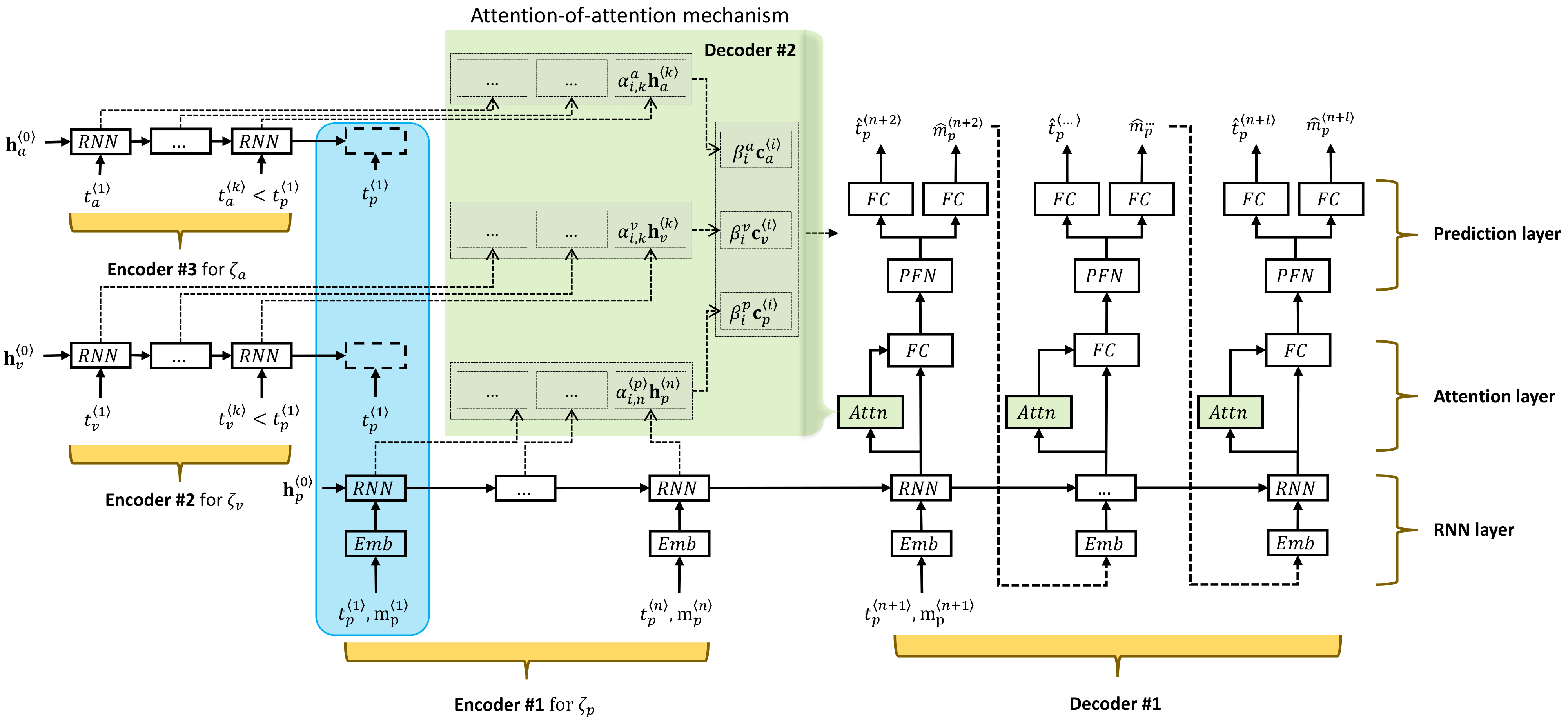
Figure 1: The architecture of PC-RNN. In addition to the patent citation chain which can only be observed during a short time window, the source-side RNN models take into account two other temporal processes which are assumed to play a critical role in modeling future citations of a patent: (1) the historical citations of the target patent’s assignee managed by “Encoder #3”, and (2) the historical citations of the target patent’s inventor encoded by “Encoder #2”. The target-side model consists of three sublayers: (1) the RNN layer which decodes the encoded sequence from source-side “Encoder #1”, (2) the attention layer which takes care about the intervening dependency structure across three sequences on source-side, and (3) the prediction layer which makes prediction for both the time and the category of the next forward patent citation.

In this section, we present our proposed model, PC-RNN, which tackles the problem of forecasting the next $l$ citations of a target patent. First, we show an overview of the design of the proposed framework. Then we detail the RNN architecture used on the source-side and the target-side of our model. Next we introduce the attention-of-attention mechanism which plays an important role in fusing multiple encoded sequences from the source-side for generating the predicted citation sequence. Finally, we describe the training procedure which unifies the distinct components of the proposed framework.

3.1 Model Overview

The chain of forward citations for a patent can be modeled as a marked temporal point process where the joint distribution of all citations received for a target paper $p$ can be described as the joint density

$$f(S_{p}) =\prod_{k}f\left((t_{p}^{\langle k\rangle},m_{p}^{\langle k\rangle})|\mathcal{H}^{\langle k\rangle}\right)$$ (1)

where $\mathcal{H}^{\langle k\rangle}$ denotes all the historical information associated with the target patent at timestamp $k$, $t_{p}^{\langle k\rangle}$ is the timestamp when the $k$-th citation arrives, and $m_{p}^{\langle k\rangle}$ is the category of the arriving citation. Because our primary use case is to make predictions in the early stages of a patent’s life cycle, we compensate for having a short observation window by incorporating citation sequences for the assignees and inventors associated with the target patent. In particular, taking as inputs (1) a time-dependent citation sequence of $n$ observations of the target patent $\zeta_{p}=\{(t_{p}^{\langle 1\rangle},m_{p}^{\langle 1\rangle}),\ldots,(t_{p}^{\langle n\rangle},m_{p}^{\langle n\rangle})\}$, (2) records of citations received by associated assignees $\zeta_{a}=\{t_{a}^{\langle k\rangle}|t_{a}^{\langle k\rangle}<t_{p}^{\langle 1\rangle}\}$, and (3) records of citations received by associated inventors $\zeta_{v}=\{t_{v}^{\langle k\rangle}|t_{v}^{\langle k\rangle}<t_{p}^{\langle 1\rangle}\}$, the task of the proposed model is to learn an optimal distribution on observations:

$$\Pr\left((t_{p}^{\langle n+1\rangle},m_{p}^{\langle n+1\rangle}),\ldots,(t_{p}^{\langle n+l\rangle},m_{p}^{\langle n+l\rangle})|\zeta_{p},\zeta_{a},\zeta_{v}\right),$$ (2)

where $\zeta_{p}$, $\zeta_{a}$, and $\zeta_{v}$ together compose the observed historical information.

Generally speaking, Eq. 2 transforms the three given sequences into another sequence. Thus, we are guided by the sequence-to-sequence paradigm Sutskever et al. (2014) to design the proposed framework. In the overview of proposed model depicted in Fig. 1, the module that handles input sequences is called source-side and the module that makes predictions is called target-side. On the source-side, three RNNs act as encoders to separately encode the observations $\zeta_{p},\zeta_{a},\zeta_{v}$ which align at timestamp $t_{p}^{\langle 1\rangle}$ when the first citation of target patent arrives. In Fig. 1, three input sequences $\zeta_{p},\zeta_{a},\zeta_{v}$ are managed by “Encoder #1”, “Encoder #2”, and “Encoder #3,” respectively. On the target-side, the decoder recurrently forecasts the time at which a new patent will cite the target patent and in which category that new patent will be. The target-side consists of three sublayers: a RNN layer, an attention layer, and a prediction layer. In particular, the RNN layer decodes the patent citation sequence from the source-side. The hidden state of the RNN layer enters the attention layer where an attentional hidden state is computed by fusing all the information embedded by the encoders. Finally, the prediction layer makes category and timestamp predictions.

3.2 Ingredients of PC-RNN

The three encoder RNNs separately handle the observed sequences $\zeta_{p},\zeta_{a},\zeta_{v}$ by compiling the inputs into an intermediate fixed-dimensional hidden representation. As an example, we describe the patent sequence encoder to illustrate the computation process. For the patent sequence, at the $k$-th observation of $\zeta_{p}$, the category information $m_{p}^{\langle k\rangle}$ of the citing patent is first projected into a dense representation through an embedding layer and then fed into the RNN along with temporal features:

$$\boldsymbol{\mathrm{h}}_{p}^{\langle k\rangle}=\sigma_{p}\left(\boldsymbol{\mathrm{W}}^{t}\boldsymbol{\mathrm{t}}_{p}^{\langle k\rangle}+\boldsymbol{\mathrm{W}}^{m}\boldsymbol{\mathrm{m}}_{p}^{\langle k\rangle}+\boldsymbol{\mathrm{W}}^{h}\boldsymbol{\mathrm{h}}_{p}^{\langle k-1\rangle}+\boldsymbol{\mathrm{b}}^{h}\right),$$ (3)

where $\boldsymbol{\mathrm{t}}_{p}^{\langle k\rangle}$ represents the temporal features (e.g., $t_{p}^{\langle k\rangle}-t_{p}^{\langle k-1\rangle}$), $\boldsymbol{\mathrm{m}}_{p}^{\langle k\rangle}$ is a dense representation of the category information, $\boldsymbol{\mathrm{h}}_{p}^{\langle k-1\rangle}$ is a $d_{p}$-dimensional hidden state from the last step which embedded historical information, and $\sigma_{p}$ is the activation function. For clarity, we use the vanilla RNN in Eq. 3 to illustrate the computation process. In practice, we use multi-layered bidirectional LSTMs Hochreiter and Schmidhuber (1997) which can capture long range temporal dependencies in sequences. In this case, at each step $k$ the output of the encoder is the summation of the hidden state of LSTMs from two directions: $\boldsymbol{\mathrm{o}}_{p}^{\langle k\rangle}=\overrightarrow{\boldsymbol{\mathrm{h}}}_{p}^{\langle k\rangle}+\overleftarrow{\boldsymbol{\mathrm{h}}}_{p}^{\langle k\rangle}$. The assignee sequence encoder for $\zeta_{a}$ and the inventor sequence encoder for $\zeta_{v}$ share similar computational processes with the target patent sequence encoder except that there is no category information to embed. The workflow of patent, inventor, and assignee encoders is depicted in Fig. 1 as “Encoder #1”, “Encoder #2”, and “Encoder #3,” respectively. On the target-side, the decoder RNN employs multi-layered unidirection LSTMs, which adds the restriction that the input point at each step is always the output from the last step.

3.2.1 Attention Layer

Theoretically, the decoder layer generates a citation sequence by recurrently maximizing the conditional probability

$$\Pr\left(t_{p}^{\langle i\rangle},m_{p}^{\langle i\rangle}|\boldsymbol{\mathrm{h}}_{d}^{\langle i\rangle},\zeta_{p},\zeta_{a},\zeta_{v}\right),i>n,$$ (4)

where $\boldsymbol{\mathrm{h}}_{d}^{\langle i\rangle}$ is the hidden state of the decoder RNN at time step $i$. However, an RNN layer alone cannot appropriately handle the conditional dependency over the three citation sequences $\zeta_{p},\zeta_{a},\zeta_{v}$. Thus, we propose an attention layer on top of the RNN layer. In particular, our model includes a two-level attention mechanism Bahdanau et al. (2014); Luong et al. (2015). First, for each time step $i$ in the decoder, a context vector is computed for each encoder RNN using all the encoder’s outputs and the current hidden state of the decoder $\boldsymbol{\mathrm{h}}_{d}^{\langle i\rangle}$. Using outputs from patent encoder as an example, the computation process is defined as:

$$\boldsymbol{\mathrm{c}}_{p}^{\langle i\rangle} =\sum_{j\in\zeta_{p}}\alpha_{i,j}^{p}\boldsymbol{\mathrm{o}}_{p}^{\langle j\rangle},$$ (5)

$$\alpha_{i,j}^{p} =\frac{\exp(e_{i,j})}{\sum_{k\in\zeta_{p}}\exp(e_{i,k})},$$

$$e_{i,j} =g(\boldsymbol{\mathrm{h}}_{d}^{\langle i\rangle},\boldsymbol{\mathrm{o}}_{p}^{\langle j\rangle})=\boldsymbol{\mathrm{V}}^{p}\tanh(\boldsymbol{\mathrm{W}}^{p}[\boldsymbol{\mathrm{h}}_{d}^{\langle i\rangle};\boldsymbol{\mathrm{o}}_{p}^{\langle i\rangle}]),$$

where $\boldsymbol{\mathrm{o}}_{p}^{\langle j\rangle}$ are encoder’s outputs, $\alpha_{i,j}^{p}$ are the attention weights, $g(\cdot)$ is an alignment function calculating the alignment weights between position $j$ of the encoder and the $i$-th position of the decoder, and $\boldsymbol{\mathrm{V}}^{p},\boldsymbol{\mathrm{W}}^{p}$ are parameters to learn. Of the four alignment functions provided in Luong et al. (2015), we use the “concat” function here because, in our case, source-side encoders output multiple sequences of different dimensions than the decoder’s hidden state. In our experiments, the dimension of the hidden state of the patent sequence encoder and decoder is set to 32 and is 16 for assignee and inventor sequence encoders. In this step, the decoder can learn to attend to certain units of each encoder which enables the model to learn complicated dependency structures. Next, the attention weights for each context vector are calculated, based on which weighted context vectors are concatenated as the input to the next layer:

$$\bar{\boldsymbol{\mathrm{c}}}^{\langle i\rangle} =[\beta_{i}^{p}\boldsymbol{\mathrm{c}}_{p}^{\langle i\rangle};\beta_{i}^{a}\boldsymbol{\mathrm{c}}_{a}^{\langle i\rangle};\beta_{i}^{v}\boldsymbol{\mathrm{c}}_{v}^{\langle i\rangle}],$$ (6)

where the calculation of $\beta$ is similar to the calculation of $\alpha$ in Eq. 5. We perform this additional attention calculation because we want the model to dynamically learn and determine the combination of context vectors from each encoder which should enhance the flexibility of the modeled memory dependency structure. We call this two-step operation an attention-of-attention mechanism. It is depicted in the green rectangle labeled “Decoder #2” in Fig. 1. Finally, the concatenated context vector $\bar{\boldsymbol{\mathrm{c}}}^{\langle i\rangle}$ is combined with hidden state $\boldsymbol{\mathrm{h}}_{d}^{\langle i\rangle}$ to generate the attentional hidden state $\bar{\boldsymbol{\mathrm{h}}}_{d}^{\langle i\rangle}$ which flows to the next prediction layer:

$$\bar{\boldsymbol{\mathrm{h}}}_{d}^{\langle i\rangle} =\phi\left(\boldsymbol{\mathrm{V}}^{c}[\bar{\boldsymbol{\mathrm{c}}}^{\langle i\rangle};\boldsymbol{\mathrm{h}}_{d}^{\langle i\rangle}]\right),$$ (7)

where $\phi$ is a non-linear activation function, and $\boldsymbol{\mathrm{V}}^{c}$ is the parameter to learn. In our experiments, we use ReLU activation function.

3.2.2 Prediction Layer

In the prediction layer, for each position in the attentional hidden state $\bar{\boldsymbol{\mathrm{h}}}_{d}^{\langle i\rangle}$, two linear transformations are applied with a non-linear activation $\varrho$ in between to further enhance the model’s capability:

$$\mathrm{PFN}(h)=w^{h2}\varrho\left(w^{h1}h+b^{h1}\right)+b^{h2},$$ (8)

where $h$ is one position in $\bar{\boldsymbol{\mathrm{h}}}_{d}^{\langle i\rangle}$, and $w^{h1},w^{h2},b^{1},b^{2}$ are parameters to learn. The output of this layer is denoted by $\tilde{\boldsymbol{\mathrm{h}}}_{d}^{\langle i\rangle}$. This operation was introduced in Vaswani et al. (2017) which is equivalent to two $1$-by-$1$ convolutions which is also called the “network in network” concept in Lin et al. (2013). In our experiments, $\varrho$ is a ReLU function. Finally, we use two fully connected layers to generate predictions:

$$\hat{t}^{\langle i+1\rangle} =\max\left(\boldsymbol{\mathrm{W}}^{t}\tilde{\boldsymbol{\mathrm{h}}}_{d}^{\langle i\rangle}+b^{t},0\right),$$ (9)

$$\hat{\boldsymbol{\mathrm{m}}}^{\langle i+1\rangle} =\mathrm{softmax}\left(\boldsymbol{\mathrm{W}}^{m}\tilde{\boldsymbol{\mathrm{h}}}_{d}^{\langle i\rangle}+b^{m}\right).$$

The total loss is the sum of the time prediction loss and the cross-entropy loss for the patent category prediction:

$$\mathcal{L} =-\sum_{j=1}^{l}\left(\log\Pr((t_{p}^{\langle n+j\rangle},m_{p}^{\langle n+j\rangle}))\right)$$ (10)

$$=-\sum_{j=1}^{l}\left(\log{\hat{\boldsymbol{\mathrm{m}}}_{\kappa}^{\langle n+j\rangle}}+\vartheta(\hat{t}^{\langle n+j\rangle},t^{\langle n+j\rangle})\right),$$

where $n$ refers to the number of points in the sequence used as observations, $l$ is the number of predictions to make, $\kappa=m^{\langle n+j\rangle}$ indexes the target category and consequently $\hat{\boldsymbol{\mathrm{m}}}_{\kappa}^{\langle n+j\rangle}$ is the probability of predicting the correct category in prediction $\boldsymbol{\mathrm{m}}^{\langle n+j\rangle}$, and $\vartheta(\cdot)$ is defined as the absolute distance between $\hat{t}^{\langle n+j\rangle}$ and $t^{\langle n+j\rangle}$. We adopted the ADAM Kingma and Ba (2014) optimizer for training.

4 Experiments

We compare our PC-RNN experimentally to state-of-the-art methods for modeling marked temporal point processes on a large patent citation dataset collected from USPTO. The results show that PC-RNN outperforms the others at modeling citation dynamics.

4.1 Dataset Description and Experiment Setup

Dataset: Our dataset originates from the publicly accessible PatentsView database which contains more than $6$ million U.S. patents. According to patent law, new inventions must cite prior arts and differentiate their innovations from them. Patent citations have a high quality because citations are examined by officials before patents are granted. For each patent, we construct a forward citation chain using timestamps from the database. We remove patents with citation chains shorter than 20 or longer than 200. Long citation chains are relative rare in practice and the unbalanced sequence length may make training difficult. For each citing patent we also extract its NBER Hall et al. (2001) category information. As a result, each patent has one main category and one subcategory. In total, there are 7 main categories and 37 subcategories in the entire patent database. For each patent, we also retrieved the associated assignees and inventors from the database and compiled the related citation chains for each. For patents with multiple assignees or inventors, we selected the longest available chain to provide the most information. Finally, having assembled the dataset, we sampled 15,000 sequences of which 12,000 sequences are used for the training set and the remaining 3,000 sequences are the test set. Our dataset and code is publicly available for download.

Metrics: Following the similar procedure in Du et al. (2016); Wang et al. (2017); Xiao et al. (2017), two metrics are used to compare the performance of different tasks. For event time prediction, we used Mean Absolute Error (MAE). For both main category and subcategory prediction, we used the Accuracy metric.

Comparison Models: State-of-the-art RNN based prediction methods can be generally categorized into two classes. (1) Intensity-based RNNs represents an observed sequence with the hidden state of a recurrent neural network. They then formulate an intensity function conditioned on the hidden state to make predictions as in a typical temporal point process. (2) End-to-end RNNs avoid explicitly designated conditional intensity functions, and instead represent the mapping from input sequences to predictions implicitly within the network structure. Our method belongs to the second class. In our experiments, we compare our model against three other major peer recurrent temporal point process models of both classes, each of which predicts both the timestamp and category of arrival points using observed sequences as input:

• RMTPP Du et al. (2016): Recurrent marked temporal point process (RMTPP) is an intensity-based RNN model for general point process analysis which is able to predict both the timestamp and the type of point in an event sequence. RMTPP is not a sequence-to-sequence model, however, by directing the $k$-th output to the $(k+1)$-th input, the model can be used as a sequence generator. RMTPP only models one sequence. So, in the experiment, we feed only the patent sequence to the model as input.

• CYAN-RNN Wang et al. (2017): CYAN-RNN is an intensity-based RNN model which models a general resharing dependence in social media datasets. It can forecast the time and user of the next resharing behavior. Similarly to RMTPP, by forcing the $k$-th output to the $(k+1)$-th input, this model is used as a sequence generator for patent citation prediction. For this experiment, we use only patent citation sequences as input to generate predictions.

• IntensityRNN Xiao et al. (2017): In IntensityRNN, a time-dependent event arrival sequence and an evenly distributed background time series work together to generate predictions for the next arrival event. In experiments, the evenly distributed background time series is simulated with assignee citations which usually have a stable citation pattern. IntensityRNN is an end-to-end RNN model.

$80\%$ As Observations
Model	Main-category		Sub-category
	ACC	MAE	ACC	MAE
RMTPP	0.2316	0.0550	0.1213	0.0545
CYAN-RNN	0.2304	0.0566	0.1209	0.0546
IntensityRNN	0.6826	0.0218	0.5258	0.0220
PC-RNN	0.9498	0.0216	0.7885	0.0216
$50\%$ As Observations
Model	Main-category		Sub-category
	ACC	MAE	ACC	MAE
RMTPP	0.1743	0.1310	0.0761	0.1320
CYAN-RNN	0.2376	0.1055	0.1244	0.0987
IntensityRNN	0.6704	0.0178	0.5141	0.0177
PC-RNN	0.7885	0.0172	0.6752	0.0172
$30\%$ As Observations
Model	Main-category		Sub-category
	ACC	MAE	ACC	MAE
RMTPP	0.2404	0.1536	0.1292	0.2317
CYAN-RNN	0.2434	0.1255	0.1269	0.1310
IntensityRNN	0.6652	0.0163	0.4928	0.0167
PC-RNN	0.7778	0.0165	0.6631	0.0164
$10\%$ As Observations
Model	Main-category		Sub-category
	ACC	MAE	ACC	MAE
RMTPP	0.1769	0.3383	0.1299	0.4606
CYAN-RNN	0.2443	0.1534	0.1296	0.1533
IntensityRNN	0.6701	0.0182	0.4795	0.0167
PC-RNN	0.7362	0.0169	0.6331	0.0169

Table 1: Performance evaluation of our method and peer methods. Timestamp predictions are evaluated using MAE. Patent category predictions are evaluated using ACC. 

4.2 Results and Discussion

The motivation for our model is to use the historical forward citations of a patent’s assignees and inventors to boost the prediction performance since the observation window of the target patent is limited. Therefore, our experiment tests observation windows of different lengths. In particular, in four experiments, we use $80\%$, $50\%$, $30\%$ and $10\%$ of the patent sequence as observations. As the observation window becomes shorter, the predictive task becomes more difficult but also more salient for real world applications. In each experiment, to fully examine each model’s performance at category prediction, each model runs the following two tasks separately:

• prediction of the timestamp and the NBER main category of the newly arrived citation.

• prediction of the timestamp and the NBER subcategory of the newly arrived citation.

Experiments are conducted with the test dataset which is separate from the training set. Results are reported in Table 1. We consider RMTPP and CYAN-RNN to be “intensity-based RNNs” because, instead of using recurrent neural nets, they treat hidden states as the embedded historical information from which they directly predict using an explicitly conditional intensity function. In contrast, IntensityRNN belongs to the end-to-end RNN model because it directly makes desired predictions given input. To better understand the experimental results, we analyze the performance of each class as compared to our model.

4.2.1 Intensity-Based Models

Our model consistently and significantly outperforms RMTPP and CYAN-RNN for category classification in all experiments. This suggests that these two models struggle to modulate patent categories and subcategories. Similar results about weak classification performance using these two models on different datasets are reported in Du et al. (2016); Wang et al. (2017). For prediction of the next forward citation, our model consistently outperforms these intensity-based models. As the observation window shrinks, the performance of our model on the category classification task decreases, though still outperforms its competitors. However, the performance of our model on the time prediction task stays relatively stable. We observe that the timestamp information contained in the assignee’s and inventor’s citation chains could help to predict upcoming citations to the target patent. In contrast, the performance of the intensity-based models on the time prediction task decreases significantly as the available observations are reduced. We observe that the optimizations for intensity-based methods is sensitive to the number of observations, especially considering that maximum likelihood estimation is used. As a result, we conclude that including sequences associated to the main target sequences in our model helps to improve its sensitivity to the number of observations.

4.2.2 End-to-End Models

Our model consistently outperforms IntensityRNN on the category classification task. In particular, for main category classification, our model is $6\%$ to $26\%$ more accurate compared to IntensityRNN across all observation windows. This improvement is even more significant for subcategory classification, where our model has an improvement of $16\%$ to $26\%$. We argue that this boost is attributed to our attention-of-attention mechanism. In our mechanism, the first attention layer allows the decoder to look back at all the hidden states for each encoder at each step and dynamically attend to only the important states in each sequence. The second attention layer empowers the model to fuse attended parts from different sequences which manages the dependencies across input sequences. In contrast, IntensityRNN relies solely on the last hidden state to carry the entire sequence’s information and the two input sequences are connected only through a fully connected layer which may cause information loss. On the time prediction task, our model outperforms IntensityRNN on most test cases, with the exception of two. Considering IntensityRNN’s poorer performance at the category classification task in those two tests, we suggest that IntensityRNN’s loss functions focus more on time loss which impacts classification performance. In contrast, the loss function in our model is more balanced and encourages the model to pay attention to the two tasks equally.

In summary, we conclude that incorporating assignee and inventor information in the source-side encoder provides extra information which improves our model’s performance at the prediction task. Additionally, as a proxy for prediction, using an end-to-end learning diagram to modulate a marked temporal point process is better than using a specific parametric form of a conditional intensity function, at least in the domain of patent citation classification. Finally, the empirical results suggest that the attention-of-attention mechanism enables the decoder to dynamically observation historical information from different input sequences and consequently enhance model performance.

5 Conclusion

In this paper, we present a patent citation dynamics model with fused attentional recurrent network. This model expands the traditional sequence-to-sequence paradigm by considering multiple sequences on the source-side: one each for the target patent, its assignee, and its inventor. We employ an attention-of-attention mechanism which encourages the decoder to attend to certain parts of each source-side sequence and then further fused the attended parts, grouping the by sequences which leverage dynamically learned weights. Our model is evaluated on on patents data collected from USPTO and experimental results demonstrate that our model can consistently outperform state-of-the-art temporal point process modeling methods at predicting time of newly arrived citations and classification of their category and subcategory.

References

- Bahdanau et al. [2014] Dzmitry Bahdanau, Kyunghyun Cho, and Yoshua Bengio. Neural machine translation by jointly learning to align and translate. arXiv preprint arXiv:1409.0473, 2014.
- Bessen [2008] James Bessen. The value of us patents by owner and patent characteristics. Research Policy, 37(5):932–945, 2008.
- Du et al. [2016] Nan Du, Hanjun Dai, Rakshit Trivedi, Utkarsh Upadhyay, Manuel Gomez-Rodriguez, and Le Song. Recurrent marked temporal point processes: Embedding event history to vector. In Proceedings of the 22nd ACM SIGKDD International Conference on Knowledge Discovery and Data Mining, pages 1555–1564. ACM, 2016.
- Filimonov and Sornette [2015] Vladimir Filimonov and Didier Sornette. Apparent criticality and calibration issues in the hawkes self-excited point process model: application to high-frequency financial data. Quantitative Finance, 15(8):1293–1314, 2015.
- Hall et al. [2001] Bronwyn H Hall, Adam B Jaffe, and Manuel Trajtenberg. The nber patent citation data file: Lessons, insights and methodological tools. Technical report, National Bureau of Economic Research, 2001.
- Hawkes [1971] Alan G Hawkes. Spectra of some self-exciting and mutually exciting point processes. Biometrika, 58(1):83–90, 1971.
- Helmstetter and Sornette [2002] Agnès Helmstetter and Didier Sornette. Subcritical and supercritical regimes in epidemic models of earthquake aftershocks. Journal of Geophysical Research: Solid Earth, 107(B10):ESE–10, 2002.
- Hochreiter and Schmidhuber [1997] Sepp Hochreiter and Jürgen Schmidhuber. Long short-term memory. Neural computation, 9(8):1735–1780, 1997.
- Isham and Westcott [1979] Valerie Isham and Mark Westcott. A self-correcting point process. Stochastic Processes and Their Applications, 8(3):335–347, 1979.
- Jang et al. [2017] Hyun Jin Jang, Han-Gyun Woo, and Changyong Lee. Hawkes process-based technology impact analysis. Journal of Informetrics, 11(2):511–529, 2017.
- Kingma and Ba [2014] Diederik P Kingma and Jimmy Ba. Adam: A method for stochastic optimization. arXiv preprint arXiv:1412.6980, 2014.
- Lee et al. [2018] Changyong Lee, Ohjin Kwon, Myeongjung Kim, and Daeil Kwon. Early identification of emerging technologies: A machine learning approach using multiple patent indicators. Technological Forecasting and Social Change, 127:291–303, 2018.
- Lin et al. [2013] Min Lin, Qiang Chen, and Shuicheng Yan. Network in network. arXiv preprint arXiv:1312.4400, 2013.
- Liu et al. [2017] Xin Liu, Junchi Yan, Shuai Xiao, Xiangfeng Wang, Hongyuan Zha, and Stephen M Chu. On predictive patent valuation: Forecasting patent citations and their types. In Thirty-First AAAI Conference on Artificial Intelligence, 2017.
- Luong et al. [2015] Minh-Thang Luong, Hieu Pham, and Christopher D Manning. Effective approaches to attention-based neural machine translation. arXiv preprint arXiv:1508.04025, 2015.
- Mishra et al. [2016] Swapnil Mishra, Marian-Andrei Rizoiu, and Lexing Xie. Feature driven and point process approaches for popularity prediction. In Proceedings of the 25th ACM International on Conference on Information and Knowledge Management, pages 1069–1078. ACM, 2016.
- Sutskever et al. [2014] Ilya Sutskever, Oriol Vinyals, and Quoc V Le. Sequence to sequence learning with neural networks. In Advances in neural information processing systems, pages 3104–3112, 2014.
- Vaswani et al. [2017] Ashish Vaswani, Noam Shazeer, Niki Parmar, Jakob Uszkoreit, Llion Jones, Aidan N Gomez, Łukasz Kaiser, and Illia Polosukhin. Attention is all you need. In Advances in Neural Information Processing Systems, pages 5998–6008, 2017.
- Von Wartburg et al. [2005] Iwan Von Wartburg, Thorsten Teichert, and Katja Rost. Inventive progress measured by multi-stage patent citation analysis. Research Policy, 34(10):1591–1607, 2005.
- Wallinga and Teunis [2004] Jacco Wallinga and Peter Teunis. Different epidemic curves for severe acute respiratory syndrome reveal similar impacts of control measures. American Journal of epidemiology, 160(6):509–516, 2004.
- Wang et al. [2017] Yongqing Wang, Huawei Shen, Shenghua Liu, Jinhua Gao, and Xueqi Cheng. Cascade dynamics modeling with attention-based recurrent neural network. In Proceedings of the 26th International Joint Conference on Artificial Intelligence, pages 2985–2991. AAAI Press, 2017.
- Xiao et al. [2016] Shuai Xiao, Junchi Yan, Changsheng Li, Bo Jin, Xiangfeng Wang, Xiaokang Yang, Stephen M Chu, and Hongyuan Zha. On modeling and predicting individual paper citation count over time. In IJCAI, pages 2676–2682, 2016.
- Xiao et al. [2017] Shuai Xiao, Junchi Yan, Xiaokang Yang, Hongyuan Zha, and Stephen M Chu. Modeling the intensity function of point process via recurrent neural networks. In Thirty-First AAAI Conference on Artificial Intelligence, 2017.