Robust Attribution Regularization

Abstract

An emerging problem in trustworthy machine learning is to train models that produce robust interpretations for their predictions. We take a step towards solving this problem through the lens of axiomatic attribution of neural networks. Our theory is grounded in the recent work, Integrated Gradients ($\operatorname{IG}$) [STY17], in axiomatically attributing a neural network’s output change to its input change. We propose training objectives in classic robust optimization models to achieve robust $\operatorname{IG}$ attributions. Our objectives give principled generalizations of previous objectives designed for robust predictions, and they naturally degenerate to classic soft-margin training for one-layer neural networks. We also generalize previous theory and prove that the objectives for different robust optimization models are closely related. Experiments demonstrate the effectiveness of our method, and also point to intriguing problems which hint at the need for better optimization techniques or better neural network architectures for robust attribution training.

1 Introduction

Trustworthy machine learning has received considerable attention in recent years. An emerging problem to tackle in this domain is to train models that produce reliable interpretations for their predictions. For example, a pathology prediction model may predict certain images as containing malignant tumor. Then one would hope that under visually indistinguishable perturbations of an image, similar sections of the image, instead of entirely different ones, can account for the prediction. However, as Ghorbani, Abid, and Zou [GAZ17] convincingly demonstrated, for existing models, one can generate minimal perturbations that substantially change model interpretations, while keeping their predictions intact. Unfortunately, while the robust prediction problem of machine learning models is well known and has been extensively studied in recent years (for example, [MMS⁺17a, SND18, WK18], and also the tutorial by Madry and Kolter [KM18]), there has only been limited progress on the problem of robust interpretations.

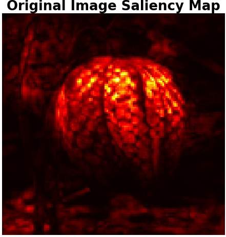
NATURAL                        IG-NORM                        IG-SUM-NORM

Top-1000 Intersection: 0.1%
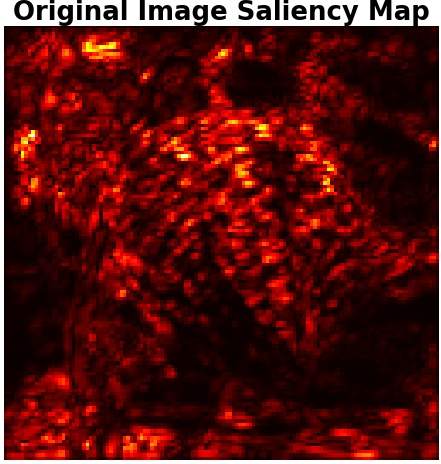
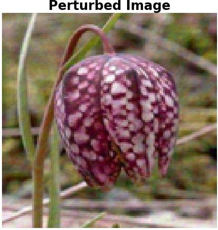
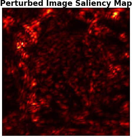
Kendall’s Correlation: 0.2607

Top-1000 Intersection: 58.8%
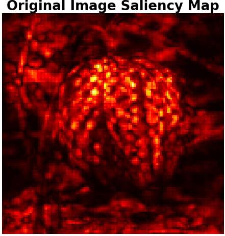
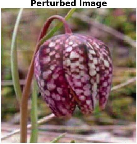
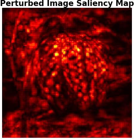
Kendall’s Correlation: 0.6736

Top-1000 Intersection: 60.1%
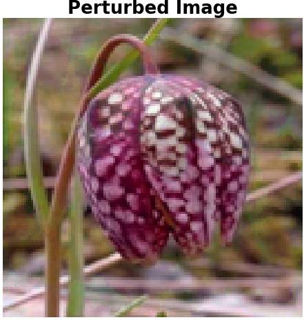
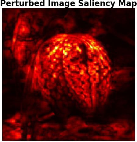
Kendall’s Correlation: 0.6951

Figure 1: Attribution robustness comparing different models. Top-1000 Intersection and Kendall’s Correlation are rank correlations between original and perturbed saliency maps. NATURAL is the naturally trained model, IG-NORM and IG-SUM-NORM are models trained using our robust attribution method. We use attribution attacks described in [GAZ17] to perturb the attributions while keeping predictions intact. For all images, the models give correct prediction – Windflower. However, the saliency maps (also called feature importance maps), computed via IG, show that attributions of the naturally trained model are very fragile, either visually or quantitatively as measured by correlation analyses, while models trained using our method are much more robust in their attributions.

In this paper we take a step towards solving this problem by viewing it through the lens of axiomatic attribution of neural networks, and propose Robust Attribution Regularization. Our theory is grounded in the recent work, Integrated Gradients ($\operatorname{IG}$) [STY17], in axiomatically attributing a neural network’s output change to its input change. Specifically, given a model $f$, two input vectors $\operatorname{{\boldsymbol{x}}},\operatorname{{\boldsymbol{x}}}^{\prime}$, and an input coordinate $i$, $\operatorname{IG}^{f}_{i}(\operatorname{{\boldsymbol{x}}},\operatorname{{\boldsymbol{x}}}^{\prime})$ defines a path integration (parameterized by a curve from $\operatorname{{\boldsymbol{x}}}$ to $\operatorname{{\boldsymbol{x}}}^{\prime}$) that assigns a number to the $i$-th input as its “contribution” to the change of the model’s output from $f(\operatorname{{\boldsymbol{x}}})$ to $f(\operatorname{{\boldsymbol{x}}}^{\prime})$. $\operatorname{IG}$ enjoys several natural theoretical properties (such as the Axiom of Completeness) that other related methods violate.

We briefly overview our approach. Given a loss function $\ell$ and a data generating distribution $P$, our Robust Attribution Regularization objective contains two parts: (1) Achieving a small loss over the distribution $P$, and (2) The $\operatorname{IG}$ attributions of the loss $\ell$ over $P$ are “close” to the $\operatorname{IG}$ attributions over $Q$, if distributions $P$ and $Q$ are close to each other. We can naturally encode these two goals in two classic robust optimization models: (1) In the uncertainty set model [BTEGN09] where we treat sample points as “nominal” points, and assume that true sample points are from certain vicinity around them, which gives:

$$\operatorname*{minimize\quad}_{\theta}\operatorname*{\mathbb{E}}_{(\operatorname{{\boldsymbol{x}}},y)\sim P}[\rho(\operatorname{{\boldsymbol{x}}},y;\theta)]$$

$$\text{where\ \ }\rho(\operatorname{{\boldsymbol{x}}},y;\theta)=\ell(\operatorname{{\boldsymbol{x}}},y;\theta)+\lambda\max_{\operatorname{{\boldsymbol{x}}}^{\prime}\in N(\operatorname{{\boldsymbol{x}}},\varepsilon)}s(\operatorname{IG}^{\ell_{y}}_{\operatorname{{\boldsymbol{h}}}}(\operatorname{{\boldsymbol{x}}},\operatorname{{\boldsymbol{x}}}^{\prime};r))$$

where $\operatorname{IG}^{\ell_{y}}_{\operatorname{{\boldsymbol{h}}}}(\cdot)$ is the attribution w.r.t. neurons in an intermediate layer $\operatorname{{\boldsymbol{h}}}$, and $s(\cdot)$ is a size function (e.g., $\|\cdot\|_{2}$) measuring the size of $\operatorname{IG}$, and (2) In the distributional robustness model [SND18, MEK15], where closeness between $P$ and $Q$ is measured using metrics such as Wasserstein distance, which gives:

$$\operatorname*{minimize\quad}_{\theta}\operatorname*{\mathbb{E}}_{P}[\ell(P;\theta)]+\lambda\sup_{Q;M\in\prod(P,Q)}\Big{\{}\operatorname*{\mathbb{E}}_{Z,Z^{\prime}}[d_{\operatorname{IG}}(Z,Z^{\prime})]\text{ s.t. }\operatorname*{\mathbb{E}}_{Z,Z^{\prime}}[c(Z,Z^{\prime})]\leq\rho\Big{\}},$$

In this formulation, $\prod(P,Q)$ is the set of couplings of $P$ and $Q$, and $M=(Z,Z^{\prime})$ is one coupling. $c(\cdot,\cdot)$ is a metric, such as $\|\cdot\|_{2}$, to measure the cost of an adversary perturbing $z$ to $z^{\prime}$. $\rho$ is an upper bound on the expected perturbation cost, thus constraining $P$ and $Q$ to be “close” with each together. $d_{\operatorname{IG}}$ is a metric to measure the change of attributions from $Z$ to $Z^{\prime}$, where we want a large $d_{\operatorname{IG}}$-change under a small $c$-change. The supremum is taken over $Q$ and $\prod(P,Q)$.

We provide theoretical characterizations of our objectives. First, we show that they give principled generalizations of previous objectives designed for robust predictions. Specifically, under weak instantiations of size function $s(\cdot)$, and how we estimate $\operatorname{IG}$ computationally, we can leverage axioms satisfied by $\operatorname{IG}$ to recover the robust prediction objective of [MMS⁺17a], the input gradient regularization objective of [RD18], and also the distributional robust prediction objective of [SND18]. These results provide theoretical evidence that robust prediction training can provide some control over robust interpretations. Second, for one-layer neural networks, we prove that instantiating $s(\cdot)$ as 1-norm coincides with the instantiation of $s(\cdot)$ as $\sf sum$, and further coincides with classic soft-margin training, which implies that for generalized linear classifiers, soft-margin training will robustify both predictions and interpretations. Finally, we generalize previous theory on distributional robust prediction [SND18] to our objectives, and show that they are closely related.

Through detailed experiments we study the effect of our method in robustifying attributions. On MNIST, Fashion-MNIST, GTSRB and Flower datasets, we report encouraging improvement in attribution robustness. Compared with naturally trained models, we show significantly improved attribution robustness, as well as prediction robustness. Compared with Madry et al.’s model [MMS⁺17a] trained for robust predictions, we demonstrate comparable prediction robustness (sometimes even better), while consistently improving attribution robustness. We observe that even when our training stops, the attribution regularization term remains much more significant compared to the natural loss term. We discuss this problem and point out that current optimization techniques may not have effectively optimized our objectives. These results hint at the need for better optimization techniques or new neural network architectures that are more amenable to robust attribution training.

The rest of the paper is organized as follows: Section 2 briefly reviews necessary background. Section 3 presents our framework for robustifying attributions, and proves theoretical characterizations. Section 4 presents instantiations of our method and their optimization, and we report experimental results in Section 5. Finally, Section 6 concludes with a discussion on future directions.

2 Preliminaries

Axiomatic attribution and Integrated Gradients Let $f:\operatorname{{\mathbb{R}}}^{d}\mapsto\operatorname{{\mathbb{R}}}$ be a real-valued function, and $\operatorname{{\boldsymbol{x}}}$ and $\operatorname{{\boldsymbol{x}}}^{\prime}$ be two input vectors. Given that function values changes from $f(\operatorname{{\boldsymbol{x}}})$ to $f(\operatorname{{\boldsymbol{x}}}^{\prime})$, a basic question is: “How to attribute the function value change to the input variables?” A recent work by Sundararajan, Taly and Yan [STY17] provides an axiomatic answer to this question. Formally, let $r:[0,1]\mapsto\operatorname{{\mathbb{R}}}^{d}$ be a curve such that $r(0)=\operatorname{{\boldsymbol{x}}}$, and $r(1)=\operatorname{{\boldsymbol{x}}}^{\prime}$, Integrated Gradients ($\operatorname{IG}$) for input variable $i$ is defined as the following integral:

$$\operatorname{IG}^{f}_{i}(\operatorname{{\boldsymbol{x}}},\operatorname{{\boldsymbol{x}}}^{\prime};r)=\int_{0}^{1}\frac{\partial f(r(t))}{\partial\operatorname{{\boldsymbol{x}}}_{i}}r^{\prime}_{i}(t)dt,$$ (1)

which formalizes the contribution of the $i$-th variable as the integration of the $i$-th partial as we move along curve $r$. Let $\operatorname{IG}^{f}(\operatorname{{\boldsymbol{x}}},\operatorname{{\boldsymbol{x}}}^{\prime};r)$ be the vector where the $i$-th component is $\operatorname{IG}^{f}_{i}$, then $\operatorname{IG}^{f}$ satisfies some natural axioms. For example, the Axiom of Completeness says that summing all coordinates gives the change of function value: ${\sf sum}(\operatorname{IG}^{f}(\operatorname{{\boldsymbol{x}}},\operatorname{{\boldsymbol{x}}}^{\prime};r))=\sum_{i=1}^{d}\operatorname{IG}^{f}_{i}(\operatorname{{\boldsymbol{x}}},\operatorname{{\boldsymbol{x}}}^{\prime};r)=f(\operatorname{{\boldsymbol{x}}}^{\prime})-f(\operatorname{{\boldsymbol{x}}})$. We refer readers to the paper [STY17] for other axioms $\operatorname{IG}$ satisfies.

Integrated Gradients for an intermediate layer. We can generalize the theory of $\operatorname{IG}$ to an intermediate layer of neurons. The key insight is to leverage the fact that Integrated Gradients is a curve integration. Therefore, given some hidden layer $\operatorname{{\boldsymbol{h}}}=[h_{1},\dots,h_{l}]$, computed by a function $h(\operatorname{{\boldsymbol{x}}})$ induced by previous layers, one can then naturally view the previous layers as inducing a curve $h\circ r$ which moves from $h(\operatorname{{\boldsymbol{x}}})$ to $h(\operatorname{{\boldsymbol{x}}}^{\prime})$, as we move from $\operatorname{{\boldsymbol{x}}}$ to $\operatorname{{\boldsymbol{x}}}^{\prime}$ along curve $r$. Viewed this way, we can thus naturally compute $\operatorname{IG}$ for $\operatorname{{\boldsymbol{h}}}$ in a way that leverages all layers of the network,

Lemma 1.

Under curve $r:[0,1]\mapsto\operatorname{{\mathbb{R}}}^{d}$ such that $r(0)=\operatorname{{\boldsymbol{x}}}$ and $r(1)=\operatorname{{\boldsymbol{x}}}^{\prime}$ for moving $\operatorname{{\boldsymbol{x}}}$ to $\operatorname{{\boldsymbol{x}}}^{\prime}$, and the function induced by layers before $\operatorname{{\boldsymbol{h}}}$, the attribution for $h_{i}$ for a differentiable $f$ is

$$\operatorname{IG}^{f}_{h_{i}}(\operatorname{{\boldsymbol{x}}},\operatorname{{\boldsymbol{x}}}^{\prime})=\sum_{j=1}^{d}\left\{\int_{0}^{1}\frac{\partial f(h(r(t)))}{\partial h_{i}}\frac{\partial h_{i}(r(t))}{\partial\operatorname{{\boldsymbol{x}}}_{j}}r^{\prime}_{j}(t)dt\right\}.$$ (2)

The corresponding summation approximation is:

$$\operatorname{IG}^{f}_{h_{i}}(\operatorname{{\boldsymbol{x}}},\operatorname{{\boldsymbol{x}}}^{\prime})=\frac{1}{m}\sum_{j=1}^{d}\left\{\sum_{k=0}^{m-1}\frac{\partial f(h(r(k/m)))}{\partial h_{i}}\frac{\partial h_{i}(r(k/m))}{\partial\operatorname{{\boldsymbol{x}}}_{j}}r^{\prime}_{j}(k/m)\right\}$$ (3)

3 Robust Attribution Regularization

In this section we propose objectives for achieving robust attribution, and study their connections with existing robust training objectives. At a high level, given a loss function $\ell$ and a data generating distribution $P$, our objectives contain two parts: (1) Achieving a small loss over the data generating distribution $P$, and (2) The $\operatorname{IG}$ attributions of the loss $\ell$ over $P$ are “close” to the $\operatorname{IG}$ attributions over distribution $Q$, if $P$ and $Q$ are close to each other. We can naturally encode these two goals in existing robust optimization models. Below we do so for two popular models: the uncertainty set model and the distributional robustness model.

3.1 Uncertainty Set Model

In the uncertainty set model, for any sample $(\operatorname{{\boldsymbol{x}}},y)\sim P$ for a data generating distribution $P$, we think of it as a “nominal” point and assume that the real sample comes from a neighborhood around $\operatorname{{\boldsymbol{x}}}$. In this case, given any intermediate layer $\operatorname{{\boldsymbol{h}}}$, we propose the following objective function:

$$\begin{split}&\operatorname*{minimize\quad}_{\theta}\operatorname*{\mathbb{E}}_{(\operatorname{{\boldsymbol{x}}},y)\sim P}[\rho(\operatorname{{\boldsymbol{x}}},y;\theta)]\\ &\text{where\ \ }\rho(\operatorname{{\boldsymbol{x}}},y;\theta)=\ell(\operatorname{{\boldsymbol{x}}},y;\theta)+\lambda\max_{\operatorname{{\boldsymbol{x}}}^{\prime}\in N(\operatorname{{\boldsymbol{x}}},\varepsilon)}s(\operatorname{IG}^{\ell_{y}}_{\operatorname{{\boldsymbol{h}}}}(\operatorname{{\boldsymbol{x}}},\operatorname{{\boldsymbol{x}}}^{\prime};r))\end{split}$$ (4)

where $\lambda\geq 0$ is a regularization parameter, $\ell_{y}$ is the loss function with label $y$ fixed: $\ell_{y}(\operatorname{{\boldsymbol{x}}};\theta)=\ell(\operatorname{{\boldsymbol{x}}},y;\theta)$, $r:[0,1]\mapsto\operatorname{{\mathbb{R}}}^{d}$ is a curve parameterization from $\operatorname{{\boldsymbol{x}}}$ to $\operatorname{{\boldsymbol{x}}}^{\prime}$, and $\operatorname{IG}^{\ell_{y}}$ is the integrated gradients of $\ell_{y}$, and therefore gives attribution of changes of $\ell_{y}$ as we go from $\operatorname{{\boldsymbol{x}}}$ to $\operatorname{{\boldsymbol{x}}}^{\prime}$. $s(\cdot)$ is a size function that measures the “size” of the attribution.

We now study some particular instantiations of the objective (4). Specifically, we recover existing robust training objectives under weak instantiations (such as choosing $s(\cdot)$ as summation function, which is not metric, or use crude approximation of $\operatorname{IG}$), and also derive new instantiations that are natural extensions to existing ones.

Proposition 1 (Madry et al.’s robust prediction objective).

If we set $\lambda=1$ , and let $s(\cdot)$ be the $\sf sum$ function (sum all components of a vector), then for any curve $r$ and any intermediate layer $\operatorname{{\boldsymbol{h}}}$, (4) is exactly the objective proposed by Madry et al. [MMS⁺17a] where $\rho(\operatorname{{\boldsymbol{x}}},y;\theta)=\max_{\operatorname{{\boldsymbol{x}}}^{\prime}\in N(\operatorname{{\boldsymbol{x}}},\varepsilon)}\ell(\operatorname{{\boldsymbol{x}}}^{\prime},y;\theta)$.

We note that: (1) $\sf sum$ is a weak size function which does not give a metric. (2) As a result, while this robust prediction objective falls within our framework, and regularizes robust attributions, it allows a small regularization term where attributions actually change significantly but they cancel each other in summation. Therefore, the control over robust attributions can be weak.

Proposition 2 (Input gradient regularization).

For any $\lambda^{\prime}>0$ and $q\geq 1$, if we set $\lambda=\lambda^{\prime}/\varepsilon^{q}$, $s(\cdot)=\|\cdot\|_{1}^{q}$, and use only the first term of summation approximation (3) to approximate $\operatorname{IG}$, then (4) becomes exactly the input gradient regularization of Drucker and LeCun [DL92], where we have $\rho(\operatorname{{\boldsymbol{x}}},y;\theta)=\ell(\operatorname{{\boldsymbol{x}}},y;\theta)+\lambda\|\nabla_{\operatorname{{\boldsymbol{x}}}}\ell(\operatorname{{\boldsymbol{x}}},y;\theta)\|_{q}^{q}$.

In the above we have considered instantiations of a weak size function (summation function), which recovers Madry et al.’s objective, and of a weak approximation of $\operatorname{IG}$ (picking the first term), which recovers input gradient regularization. In the next example, we pick a nontrivial size function, the 1-norm $\|\cdot\|_{1}$, use the precise $\operatorname{IG}$, but then we use a trivial intermediate layer, the output loss $\ell_{y}$.

Proposition 3 (Regularizing by attribution of the loss output).

Let us set $\lambda=1$, $s(\cdot)=\|\cdot\|_{1}$, and $\operatorname{{\boldsymbol{h}}}=\ell_{y}$ (the output layer of loss function!), then we have $\rho(\operatorname{{\boldsymbol{x}}},y;\theta)=\ell_{y}(\operatorname{{\boldsymbol{x}}})+\max_{\operatorname{{\boldsymbol{x}}}^{\prime}\in N(\operatorname{{\boldsymbol{x}}},\varepsilon)}\{|\ell_{y}(\operatorname{{\boldsymbol{x}}}^{\prime})-\ell_{y}(\operatorname{{\boldsymbol{x}}})|\}$.

We note that this loss function is a “surrogate” loss function for Madry et al.’s loss function because $\ell_{y}(\operatorname{{\boldsymbol{x}}})+\max_{\operatorname{{\boldsymbol{x}}}^{\prime}\in N(\operatorname{{\boldsymbol{x}}},\varepsilon)}\{|\ell_{y}(\operatorname{{\boldsymbol{x}}}^{\prime})-\ell_{y}(\operatorname{{\boldsymbol{x}}})|\}\geq\ell_{y}(\operatorname{{\boldsymbol{x}}})+\max_{\operatorname{{\boldsymbol{x}}}^{\prime}\in N(\operatorname{{\boldsymbol{x}}},\varepsilon)}\{(\ell_{y}(\operatorname{{\boldsymbol{x}}}^{\prime})-\ell_{y}(\operatorname{{\boldsymbol{x}}}))\}=\max_{\operatorname{{\boldsymbol{x}}}^{\prime}\in N(\operatorname{{\boldsymbol{x}}},\varepsilon)}\ell_{y}(\operatorname{{\boldsymbol{x}}}^{\prime})$. Therefore, even at such a trivial instantiation, robust attribution regularization provides interesting guarantees.

3.2 Distributional Robustness Model

A different but popular model for robust optimization is the distributional robustness model. In this case we consider a family of distributions $\operatorname{{\cal P}}$, each of which is supposed to be a “slight variation” of a base distribution $P$. The goal of robust optimization is then that certain objective functions obtain stable values over this entire family. Here we apply the same underlying idea to the distributional robustness model: One should get a small loss value over the base distribution $P$, and for any distribution $Q\in\operatorname{{\cal P}}$, the $\operatorname{IG}$-based attributions change only a little if we move from $P$ to $Q$. This is formalized as:

$$\operatorname*{minimize\quad}_{\theta}\operatorname*{\mathbb{E}}_{P}[\ell(P;\theta)]+\lambda\sup_{Q\in\operatorname{{\cal P}}}\left\{W_{d_{\operatorname{IG}}}(P,Q)\right\},$$

where the $W_{d_{\operatorname{IG}}}(P,Q)$ is the Wasserstein distance between $P$ and $Q$ under a distance metric $d_{\operatorname{IG}}$. We use $\operatorname{IG}$ to highlight that this metric is related to integrated gradients.

We propose again $d_{\operatorname{IG}}(\operatorname{{\boldsymbol{z}}},\operatorname{{\boldsymbol{z}}}^{\prime})=s(\operatorname{IG}^{\ell}_{\operatorname{{\boldsymbol{h}}}}(\operatorname{{\boldsymbol{z}}},\operatorname{{\boldsymbol{z}}}^{\prime}))$. We are particularly interested in the case where $\operatorname{{\cal P}}$ is a Wasserstein ball around the base distribution $P$, using “perturbation” cost metric $c(\cdot)$. This gives regularization term $\lambda\operatorname*{\mathbb{E}}_{W_{c}(P,Q)\leq\rho}\sup\{W_{d_{\operatorname{IG}}}(P,Q)\}$. An unsatisfying aspect of this objective, as one can observe now, is that $W_{d_{\operatorname{IG}}}$ and $W_{c}$ can take two different couplings, while intuitively we want to use only one coupling to transport $P$ to $Q$. For example, this objective allows us to pick a coupling $M_{1}$ under which we achieve $W_{d_{\operatorname{IG}}}$ (recall that Wasserstein distance is an infimum over couplings), and a different coupling $M_{2}$ under which we achieve $W_{c}$, but under $M_{1}=(Z,Z^{\prime})$, $\operatorname*{\mathbb{E}}_{z,z^{\prime}\sim M_{1}}[c(z,z^{\prime})]>\rho$, violating the constraint. This motivates the following modification:

$$\begin{split}&\operatorname*{minimize\quad}_{\theta}\operatorname*{\mathbb{E}}_{P}[\ell(P;\theta)]+\lambda\sup_{Q;M\in\prod(P,Q)}\Big{\{}\operatorname*{\mathbb{E}}_{Z,Z^{\prime}}[d_{\operatorname{IG}}(Z,Z^{\prime})]\text{ s.t. }\operatorname*{\mathbb{E}}_{Z,Z^{\prime}}[c(Z,Z^{\prime})]\leq\rho\Big{\}},\end{split}$$ (5)

In this formulation, $\prod(P,Q)$ is the set of couplings of $P$ and $Q$, and $M=(Z,Z^{\prime})$ is one coupling. $c(\cdot,\cdot)$ is a metric, such as $\|\cdot\|_{2}$, to measure the cost of an adversary perturbing $z$ to $z^{\prime}$. $\rho$ is an upper bound on the expected perturbation cost, thus constraining $P$ and $Q$ to be “close” with each together. $d_{\operatorname{IG}}$ is a metric to measure the change of attributions from $Z$ to $Z^{\prime}$, where we want a large $d_{\operatorname{IG}}$-change under a small $c$-change. The supremum is taken over $Q$ and $\prod(P,Q)$.

Proposition 4 (Wasserstein prediction robustness).

Let $s(\cdot)$ be the summation function and $\lambda=1$, then for any curve $\gamma$ and any layer $\operatorname{{\boldsymbol{h}}}$, (5) reduces to $\sup_{Q:W_{c}(P,Q)\leq\rho}\left\{\operatorname*{\mathbb{E}}_{Q}[\ell(Q;\theta)]\right\}$, which is the objective proposed by Sinha, Namhoong, and Duchi [SND18] for robust predictions.

Lagrange relaxation. For any $\gamma\geq 0$, the Lagrange relaxation of (5) is

$$\begin{split}\operatorname*{minimize\quad}_{\theta}\bigg{\{}\operatorname*{\mathbb{E}}_{P}[\ell(P;\theta)]+\lambda\sup_{Q;M\in\prod(P,Q)}\Big{\{}\operatorname*{\mathbb{E}}_{M=(Z,Z^{\prime})}\big{[}d_{\operatorname{IG}}(Z,Z^{\prime})-\gamma c(Z,Z^{\prime})\big{]}\Big{\}}\bigg{\}}\end{split}$$ (6)

where the supremum is taken over $Q$ (unconstrained) and all couplings of $P$ and $Q$, and we want to find a coupling under which $\operatorname{IG}$ attributions change a lot, while the perturbation cost from $P$ to $Q$ with respect to $c$ is small. Recall that $g:\operatorname{{\mathbb{R}}}^{d}\times\operatorname{{\mathbb{R}}}^{d}\rightarrow\operatorname{{\mathbb{R}}}$ is a normal integrand if for each $\alpha$, the mapping $z\rightarrow\{z^{\prime}|g(z,z^{\prime})\leq\alpha\}$ is closed-valued and measurable [RW09].

Our next two theorems generalize the duality theory in [SND18] to a much larger, but natural, class of objectives.

Theorem 1.

Suppose $c(z,z)=0$ and $d_{\operatorname{IG}}(z,z)=0$ for any $z$, and suppose $\gamma c(z,z^{\prime})-d_{\operatorname{IG}}(z,z^{\prime})$ is a normal integrand. Then, $\sup_{Q;M\in\prod(P,Q)}\{\operatorname*{\mathbb{E}}_{M=(Z,Z^{\prime})}[d^{\gamma}_{\operatorname{IG}}(Z,Z^{\prime})]\}=\operatorname*{\mathbb{E}}_{z\sim P}[\sup_{z^{\prime}}\{d^{\gamma}_{\operatorname{IG}}(z,z^{\prime})\}].$ Consequently, we have (6) to be equal to the following:

$$\begin{split}\operatorname*{minimize\quad}_{\theta}\operatorname*{\mathbb{E}}_{z\sim P}\Big{[}\ell(z;\theta)+\lambda\sup_{z^{\prime}}\{d_{\operatorname{IG}}(z,z^{\prime})-\gamma c(z,z^{\prime})\}\Big{]}\end{split}$$ (7)

The assumption $d_{\operatorname{IG}}(z,z)=0$ is true for what we propose, and $c(z,z)=0$ is true for any typical cost such as $\ell_{p}$ distances. The normal integrand assumption is also very weak, e.g., it is satisfied when $d_{\operatorname{IG}}$ is continuous and $c$ is closed convex.

Note that (7) and (4) are very similar, and so we use (4) for the rest the paper. Finally, given Theorem 1, we are also able to connect (5) and (7) with the following duality result:

Theorem 2.

Suppose $c(z,z)=0$ and $d_{\operatorname{IG}}(z,z)=0$ for any $z$, and suppose $\gamma c(z,z^{\prime})-d_{\operatorname{IG}}(z,z^{\prime})$ is a normal integrand. For any $\rho>0$, there exists $\gamma\geq 0$ such that the optimal solutions of (7) are optimal for (5).

3.3 One Layer Neural Networks

We now consider the special case of one-layer neural networks, where the loss function takes the form of $\ell(\operatorname{{\boldsymbol{x}}},y;\operatorname{{\boldsymbol{w}}})=g(-y\langle\operatorname{{\boldsymbol{w}}},\operatorname{{\boldsymbol{x}}}\rangle)$, $\operatorname{{\boldsymbol{w}}}$ is the model parameters, $\operatorname{{\boldsymbol{x}}}$ is a feature vector, $y$ is a label, and $g$ is nonnegative. We take $s(\cdot)$ to be $\|\cdot\|_{1}$, which corresponds to a strong instantiation that does not allow attributions to cancel each other. Interestingly, we prove that for natural choices of $g$, this is however exactly Madry et al.’s objective [MMS⁺17a], which corresponds to $s(\cdot)={\sf sum}(\cdot)$. That is, the strong ($s(\cdot)=\|\cdot\|_{1}$) and weak instantiations ($s(\cdot)={\sf sum}(\cdot)$) coincide for one-layer neural networks. This thus says that for generalized linear classifiers, “robust interpretation” coincides with “robust predictions,” and further with classic soft-margin training.

Theorem 3.

Suppose that $g$ is differentiable, non-decreasing, and convex. Then for $\lambda=1$, $s(\cdot)=\|\cdot\|_{1}$, and $\ell_{\infty}$ neighborhood, (4) reduces to Madry et al.’s objective:

$$\sum_{i=1}^{m}\max_{\|\operatorname{{\boldsymbol{x}}}^{\prime}_{i}-\operatorname{{\boldsymbol{x}}}_{i}\|_{\infty}\leq\varepsilon}g(-y_{i}\langle\operatorname{{\boldsymbol{w}}},\operatorname{{\boldsymbol{x}}}^{\prime}_{i}\rangle)\ \ \text{(Madry et al.'s objective)}$$

$$= \sum_{i=1}^{m}g(-y_{i}\langle\operatorname{{\boldsymbol{w}}},\operatorname{{\boldsymbol{x}}}_{i}\rangle+\varepsilon\|\operatorname{{\boldsymbol{w}}}\|_{1})\ \ \text{(soft-margin)}.$$

Natural losses, such as Negative Log-Likelihood and softplus hinge loss, satisfy the conditions of this theorem.

4 Instantiations and Optimizations

In this section we discuss instantiations of (4) and how to optimize them. We start by presenting two objectives instantiated from our method: (1) IG-NORM, and (2) IG-SUM-NORM. Then we discuss how to use gradient descent to optimize these objectives.

IG-NORM. As our first instantiation, we pick $s(\cdot)=\|\cdot\|_{1}$, $\operatorname{{\boldsymbol{h}}}$ to be the input layer, and $r$ to be the straightline connecting $\operatorname{{\boldsymbol{x}}}$ and $\operatorname{{\boldsymbol{x}}}^{\prime}$. This gives:

$$\operatorname*{minimize\quad}_{\theta}\operatorname*{\mathbb{E}}_{(\operatorname{{\boldsymbol{x}}},y)\sim P}\left[\ell(\operatorname{{\boldsymbol{x}}},y;\theta)+\lambda\max_{\operatorname{{\boldsymbol{x}}}^{\prime}\in N(\operatorname{{\boldsymbol{x}}},\varepsilon)}\|\operatorname{IG}^{\ell_{y}}(\operatorname{{\boldsymbol{x}}},\operatorname{{\boldsymbol{x}}}^{\prime})\|_{1}\right]$$

IG-SUM-NORM. In the second instantiation we combine the sum size function and norm size function, and define $s(\cdot)={\sf sum}(\cdot)+\beta\|\cdot\|_{1}$. Where $\beta\geq 0$ is a regularization parameter. Now with the same $\operatorname{{\boldsymbol{h}}}$ and $r$ as above, and put $\lambda=1$, then our method simplifies to:

$$\operatorname*{minimize\quad}_{\theta}\operatorname*{\mathbb{E}}_{(\operatorname{{\boldsymbol{x}}},y)\sim P}\left[\max_{\operatorname{{\boldsymbol{x}}}^{\prime}\in N(\operatorname{{\boldsymbol{x}}},\varepsilon)}\left\{\ell(\operatorname{{\boldsymbol{x}}}^{\prime},y;\theta)+\beta\|\operatorname{IG}^{\ell_{y}}(\operatorname{{\boldsymbol{x}}},\operatorname{{\boldsymbol{x}}}^{\prime})\|_{1}\right\}\right]$$

which can be viewed as appending an extra robust IG term to $\ell(\operatorname{{\boldsymbol{x}}}^{\prime})$.

Gradient descent optimization. We propose the following gradient descent framework to optimize the objectives. The framework is parameterized by an adversary $\operatorname{{\cal A}}$ which is supposed to solve the inner max by finding a point $\operatorname{{\boldsymbol{x}}}^{\star}$ which changes attribution significantly. Specifically, given a point $(\operatorname{{\boldsymbol{x}}},y)$ at time step $t$ during SGD training, we have the following two steps (this can be easily generalized to mini-batches):

Attack step. We run $\operatorname{{\cal A}}$ on $(\operatorname{{\boldsymbol{x}}},y)$ to find $\operatorname{{\boldsymbol{x}}}^{\star}$ that produces a large inner max term (that is $\|\operatorname{IG}^{\ell_{y}}(\operatorname{{\boldsymbol{x}}},\operatorname{{\boldsymbol{x}}}^{\star})\|_{1}$ for IG-NORM, and $\ell(\operatorname{{\boldsymbol{x}}}^{\star})+\beta\|\operatorname{IG}^{\ell_{y}}(\operatorname{{\boldsymbol{x}}},\operatorname{{\boldsymbol{x}}}^{\star})\|_{1}$ for IG-SUM-NORM.

Gradient step. Fixing $\operatorname{{\boldsymbol{x}}}^{\star}$, we can then compute the gradient of the corresponding objective with respect to $\theta$, and then update the model.

Important objective parameters. In both attack and gradient steps, we need to differentiate $\operatorname{IG}$ (in attack step, $\theta$ is fixed and we differentiate w.r.t. $\operatorname{{\boldsymbol{x}}}$, while in gradient step, this is reversed), and this induces a set of parameters of the objectives to tune for optimization, which is summarized in Table 1. Differentiating summation approximation of $\operatorname{IG}$ amounts to compute second partial derivatives. We rely on the auto-differentiation capability of TensorFlow [ABC⁺16] to compute second derivatives.

Adversary $\operatorname{{\cal A}}$	Adversary to find $\operatorname{{\boldsymbol{x}}}^{\star}$. Note that our goal is simply to maximize the inner term in a neighborhood, thus in this paper we choose Projected Gradient Descent for this purpose.
$m$ in the attack step	To differentiate $\operatorname{IG}$ in the attack step, we use summation approximation of $\operatorname{IG}$, and this is the number of segments for apprioximation.
$m$ in the gradient step	Same as above, but in the gradient step. We have this $m$ separately due to efficiency consideration.
$\lambda$	Regularization parameter for IG-NORM.
$\beta$	Regularization parameter for IG-SUM-NORM.

Table 1: Optimization parameters.

5 Experiments

We now perform experiments using our method. We ask the following questions: (1) Comparing models trained by our method and naturally trained models at test time, do we maintain the accuracy on unperturbed test inputs? (2) At test time, if we use attribution attacks mentioned in [GAZ17] to perturb attributions while keeping predictions intact, how does the attribution robustness of our models compare with that of the naturally trained models? (3) Finally, how do we compare attribution robustness of our models with weak instantiations for robust predictions?

To answer these questions, We perform experiments on four classic datasets: MNIST [LCB98], Fashion-MNIST [XRV17], GTSRB [SSSI12], and Flower [NZ06]. In summary, our findings are the following: (1) Our method results in very small drop in test accuracy compared with naturally trained models. (2) On the other hand, our method gives signficantly better attribution robustness, as measured by correlation analyses. (3) Finally, our models yield comparable prediction robustness (sometimes even better), while consistently improving attribution robustness. In the rest of the section we give more details.

Evaluation setup. In this work we use $\operatorname{IG}$ to compute attributions (i.e. feature importance map), which, as demonstrated by [GAZ17], is more robust compared to other related methods (note that, $\operatorname{IG}$ also enjoys other theoretical properties). To attack attribution while retaining model predictions, we use Iterative Feature Importance Attacks (IFIA) proposed by [GAZ17]. Due to lack of space, we defer details of parameters and other settings to the appendix. We use two metrics to measure attribution robustness (i.e. how similar the attributions are between original and perturbed images):

Kendall’s tau rank order correlation. Attribution methods rank all of the features in order of their importance, we thus use the rank correlation  [Ken38] to compare similarity between interpretations.

Top-k intersection. We compute the size of intersection of the $k$ most important features before and after perturbation.

Compared with [GAZ17], we use Kendall’s tau correlation, instead of Spearman’s rank correlation. The reason is that we found that on the GTSRB and Flower datasets, Spearman’s correlation is not consistent with visual inspection, and often produces too high correlations. In comparison, Kendall’s tau correlation consistently produces lower correlations and aligns better with visual inspection. Finally, when computing attribution robustness, we only consider the test samples that are correctly classified by the model.

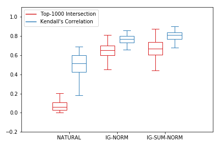
Comparing with natural models. Figures (a), (b), (c), and (d) in Figure 2 show that, compared with naturally trained models, robust attribution training gives significant improvements in attribution robustness (measured by either median or confidence intervals). The exact numbers are recorded in Table 2: Compared with naturally trained models (rows where “Approach” is NATURAL), robust attribution training has significantly better adversarial accuracy and attribution robustness, while having a small drop in natural accuracy (denoted by Nat Acc.).

(a) MNIST

(b) Fashion-MNIST

(c) GTSRB

(d) Flower

Figure 2: Experiment results on MNIST, Fashion-MNIST, GTSRB and Flower.

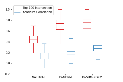
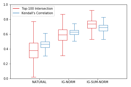
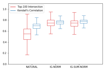
Ineffective optimization. We observe that even when our training stops, the attribution regularization term remains much more significant compared to the natural loss term. For example for IG-NORM, when training stops on MNIST, $\ell(\operatorname{{\boldsymbol{x}}})$ typically stays at  1, but $\|\operatorname{IG}(\operatorname{{\boldsymbol{x}}},\operatorname{{\boldsymbol{x}}}^{\prime})\|_{1}$ stays at $10\sim 20$. This indicates that optimization has not been very effective in minimizing the regularization term. There are two possible reasons to this: (1) Because we use summation approximation of $\operatorname{IG}$, it forces us to compute second derivatives, which may not be numerically stable for deep networks. (2) The network architecture may be inherently unsuitable for robust attributions, rendering the optimization hard to converge.

Comparing with robust prediction models. Finally we compare with Madry et al.’s models, which are trained for robust prediction. We use Adv Acc. to denote adversarial accuracy (prediction accuracy on perturbed inputs). Again, TopK Inter. denotes the average topK intersection ($K=100$ for MNIST, Fashion-MNIST and GTSRB datasets, $K=1000$ for Flower), and Rank Corr. denotes the average Kendall’s rank order correlation. Table 2 gives the details of the results. As we can see, our models give comparable adversarial accuracy, and are sometimes even better (on the Flower dataset). On the other hand, we are consistently better in terms of attribution robustness.

Dataset	Approach	Nat Acc.	Adv Acc.	TopK Inter.	Rank Corr.
MNIST	NATURAL	99.17%	0.00%	46.61%	0.1758
	Madry et al.	98.40%	92.47%	62.56%	0.2422
	IG-NORM	98.74%	81.43%	71.36%	0.2841
	IG-SUM-NORM	98.34%	88.17%	72.45%	0.3111
Fashion-MNIST	NATURAL	90.86%	0.01%	39.01%	0.4610
	Madry et al.	85.73%	73.01%	46.12%	0.6251
	IG-NORM	85.13%	65.95%	59.22%	0.6171
	IG-SUM-NORM	85.44%	70.26%	72.08%	0.6747
GTSRB	NATURAL	98.57%	21.05%	54.16%	0.6790
	Madry et al.	97.59%	83.24%	68.85%	0.7520
	IG-NORM	97.02%	75.24%	74.81%	0.7555
	IG-SUM-NORM	95.68%	77.12%	74.04%	0.7684
Flower	NATURAL	86.76%	0.00%	8.12%	0.4978
	Madry et al.	83.82%	41.91%	55.87%	0.7784
	IG-NORM	85.29%	24.26%	64.68%	0.7591
	IG-SUM-NORM	82.35%	47.06%	66.33%	0.7974

Table 2: Experiment results including prediction accuracy, prediction robustness and attribution robustness.

6 Discussion and Conclusion

This paper builds a theory to robustify model interpretations through the lens of axiomatic attributions of neural networks. We show that our theory gives principled generalizations of previous formulations for robust predictions, and we characterize our objectives for one-layer neural networks. We believe that our work opens many intriguing avenues for future research, and we discuss a few topics below.
Why we want robust attributions? Model attributions are facts about model behaviors. While robust attribution does not necessarily mean that the attribution is correct, a model with brittle attribution can never be trusted. To this end, it seems interesting to examine attribution methods other than Integrated Gradients.
Robust attribution leads to more human-aligned attribution. Note that our proposed training scheme requires both prediction correctness and robust attributions, and therefore it encourages to learn invariant features from data that are also highly predictive. In our experiments, we found an intriguing phenomenon that our regularized models produce attributions that are much more aligned with human perceptions (for example, see Figure 1). Our results are aligned with the recent work [TSE⁺19, EIS⁺19].
Robust attribution may help tackle spurious correlations. In view of our discussion so far, we think it is plausible that robust attribution regularization can help remove spurious correlations because intuitively spurious correlations should not be able to be reliably attributed to. Future research on this potential connection seems warranted.
Difficulty of optimization. While our experimental results are encouraging, we observe that when training stops, the attribution regularization term remains significant (typically around tens to hundreds), which indicates ineffective optimization for the objectives. To this end, a main problem is network depth, where as depth increases, we get very unstable trajectories of gradient descent, which seems to be related to the use of second order information during robust attribution optimization (due to summation approximation, we have first order terms in the training objectives). Therefore, it is natural to further study better optimization tchniques or better architectures for robust attribution training.

7 Acknowledgments

This work is partially supported by Air Force Grant FA9550-18-1-0166, the National Science Foundation (NSF) Grants CCF-FMitF-1836978, SaTC-Frontiers-1804648 and CCF-1652140 and ARO grant number W911NF-17-1-0405.

Appendix A Code

Code for this paper is publicly available at the following repository:
https://github.com/jfc43/robust-attribution-regularization

Appendix B Proofs

B.1 Additional definitions

Let $P,Q$ be two distributions, a coupling $M=(Z,Z^{\prime})$ is a joint distribution, where, if we marginalize $M$ to the first component, $Z$, it is identically distributed as $P$, and if we marginalize $M$ to the second component, $Z^{\prime}$, it is identically distributed as $Q$. Let $\prod(P,Q)$ be the set of all couplings of $P$ and $Q$, and let $c(\cdot,\cdot)$ be a “cost” function that maps $(z,z^{\prime})$ to a real value. Wasserstein distance between $P$ and $Q$ w.r.t. $c$ is defined as

$$W_{c}(P,Q)=\inf_{M\in\prod(P,Q)}\left\{\operatorname*{\mathbb{E}}_{(z,z^{\prime})\sim M}\left[c(z,z^{\prime})\right]\right\}.$$

Intuitively, this is to find the “best transportation plan” (a coupling $M$) to minimize the expected transportation cost (transporting $z$ to $z^{\prime}$ where the cost is $c(z,z^{\prime})$).

B.2 Integrated Gradients for an Intermediate Layer

In this section we show how to compute Integrated Gradients for an intermediate layer of a neural network. Let $h:\operatorname{{\mathbb{R}}}^{d}\mapsto\operatorname{{\mathbb{R}}}^{k}$ be a function that computes a hidden layer of a neural network, where we map a $d$-dimensional input vector to a $k$-dimensional output vector. Given two points $\operatorname{{\boldsymbol{x}}}$ and $\operatorname{{\boldsymbol{x}}}^{\prime}$ for computing attribution, again we consider a parameterization (which is a mapping $r:\operatorname{{\mathbb{R}}}\mapsto\operatorname{{\mathbb{R}}}^{d}$) such that $r(0)=\operatorname{{\boldsymbol{x}}}$, and $r(1)=\operatorname{{\boldsymbol{x}}}^{\prime}$.

The key insight is to leverage the fact that Integrated Gradients is a curve integration. Therefore, given some hidden layer, one can then naturally view the previous layers as inducing a curve $h\circ r$ which moves from $h(\operatorname{{\boldsymbol{x}}})$ to $h(\operatorname{{\boldsymbol{x}}}^{\prime})$, as we move from $\operatorname{{\boldsymbol{x}}}$ to $\operatorname{{\boldsymbol{x}}}^{\prime}$ along curve $r$. Viewed this way, we can thus naturally compute $\operatorname{IG}$ for $\operatorname{{\boldsymbol{h}}}$ in a way that leverages all layers of the network. Specifically, consider another curve $\gamma(t):\operatorname{{\mathbb{R}}}\mapsto\operatorname{{\mathbb{R}}}^{k}$, defined as $\gamma(t)=h(r(t))$, to compute a curve integral. By definition we have $f(\operatorname{{\boldsymbol{x}}})=g(h(\operatorname{{\boldsymbol{x}}}))$

$$f(\operatorname{{\boldsymbol{x}}}^{\prime})-f(\operatorname{{\boldsymbol{x}}}) =g(h(\operatorname{{\boldsymbol{x}}}^{\prime}))-g(h(\operatorname{{\boldsymbol{x}}}))$$

$$=g(\gamma(1))-g(\gamma(0))$$

$$=\int_{0}^{1}\sum_{i=1}^{k}\frac{\partial f(\gamma(t))}{\partial h_{i}}\gamma_{i}^{\prime}(t)dt$$

$$=\sum_{i=1}^{k}\int_{0}^{1}\frac{\partial f(\gamma(t))}{\partial h_{i}}\gamma_{i}^{\prime}(t)dt$$

Therefore we can define the attribution of $h_{i}$ naturally as

$$\operatorname{IG}^{f}_{h_{i}}(\operatorname{{\boldsymbol{x}}},\operatorname{{\boldsymbol{x}}}^{\prime})=\int_{0}^{1}\frac{\partial f(\gamma(t))}{\partial h_{i}}\gamma_{i}^{\prime}(t)dt$$

Let’s unpack this a little more:

$$\int_{0}^{1}\frac{\partial f(\gamma(t))}{\partial h_{i}}\gamma_{i}^{\prime}(t)dt =\int_{0}^{1}\frac{\partial f(h(r(t)))}{\partial h_{i}}\sum_{j=1}^{d}\frac{\partial h_{i}(r(t))}{\partial\operatorname{{\boldsymbol{x}}}_{j}}r_{j}^{\prime}(t)dt$$

$$=\int_{0}^{1}\frac{\partial f(h(r(t)))}{\partial h_{i}}\sum_{j=1}^{d}\frac{\partial h_{i}(r(t))}{\partial\operatorname{{\boldsymbol{x}}}_{j}}r_{j}^{\prime}(t)dt$$

$$=\sum_{j=1}^{d}\left\{\int_{0}^{1}\frac{\partial f(h(r(t)))}{\partial h_{i}}\frac{\partial h_{i}(r(t))}{\partial\operatorname{{\boldsymbol{x}}}_{j}}r_{j}^{\prime}(t)dt\right\}$$

This thus gives the lemma

Lemma 2.

Under curve $r:\operatorname{{\mathbb{R}}}\mapsto\operatorname{{\mathbb{R}}}^{d}$ where $r(0)=\operatorname{{\boldsymbol{x}}}$ and $r(1)=\operatorname{{\boldsymbol{x}}}^{\prime}$, the attribution for $h_{i}$ for a differentiable function $f$ is

$$\operatorname{IG}^{f}_{h_{i}}(\operatorname{{\boldsymbol{x}}},\operatorname{{\boldsymbol{x}}}^{\prime},r)=\sum_{j=1}^{d}\left\{\int_{0}^{1}\frac{\partial f(h(r(t)))}{\partial h_{i}}\frac{\partial h_{i}(r(t))}{\partial\operatorname{{\boldsymbol{x}}}_{j}}r^{\prime}_{j}(t)dt\right\}$$ (8)

Note that (6) nicely recovers attributions for input layer, in which case $h$ is the identity function. Summation approximation. Similarly, we can approximate the above Riemann integral using a summation. Suppose we slice $[0,1]$ into $m$ equal segments, then (2) can be approximated as:

$$\operatorname{IG}^{f}_{h_{i}}(\operatorname{{\boldsymbol{x}}},\operatorname{{\boldsymbol{x}}}^{\prime})=\frac{1}{m}\sum_{j=1}^{d}\left\{\sum_{k=0}^{m-1}\frac{\partial f(h(r(k/m)))}{\partial h_{i}}\frac{\partial h_{i}(r(k/m))}{\partial\operatorname{{\boldsymbol{x}}}_{j}}r^{\prime}_{j}(k/m)\right\}$$ (9)

B.3 Proof of Proposition 1

If we put $\lambda=1$ and let $s(\cdot)$ be the $\sf sum$ function (sum all components of a vector), then for any curve $r$ and any intermediate layer $\operatorname{{\boldsymbol{h}}}$, (4) becomes:

$$\rho(\operatorname{{\boldsymbol{x}}},y;\theta) =\ell(\operatorname{{\boldsymbol{x}}},y;\theta)+\max_{\operatorname{{\boldsymbol{x}}}^{\prime}\in N(\operatorname{{\boldsymbol{x}}},\varepsilon)}\{{\sf sum}(\operatorname{IG}^{\ell_{y}}(\operatorname{{\boldsymbol{x}}},\operatorname{{\boldsymbol{x}}}^{\prime};r))\}$$

$$=\ell(\operatorname{{\boldsymbol{x}}},y;\theta)+\max_{\operatorname{{\boldsymbol{x}}}^{\prime}\in N(\operatorname{{\boldsymbol{x}}},\varepsilon)}\{\ell(\operatorname{{\boldsymbol{x}}}^{\prime},y;\theta)-\ell(\operatorname{{\boldsymbol{x}}},y;\theta)\}$$

$$=\max_{\operatorname{{\boldsymbol{x}}}^{\prime}\in N(\operatorname{{\boldsymbol{x}}},\varepsilon)}\ell(\operatorname{{\boldsymbol{x}}}^{\prime},y;\theta)$$

where the second equality is due to the Axiom of Completeness of $\operatorname{IG}$.

B.4 Proof of Proposition 2

Input gradient regularization is an old idea proposed by Drucker and LeCun [DL92], and is recently used by Ross and Doshi-Velez [RD18] in adversarial training setting. Basically, for $q\geq 1$, they propose $\rho(\operatorname{{\boldsymbol{x}}},y;\theta)=\ell(\operatorname{{\boldsymbol{x}}},y;\theta)+\lambda\|\nabla_{\operatorname{{\boldsymbol{x}}}}\ell(\operatorname{{\boldsymbol{x}}},y;\theta)\|_{q}^{q},$ where they want small gradient at $\operatorname{{\boldsymbol{x}}}$. To recover this objective from robust attribution regularization, let us pick $s(\cdot)$ as the $\|\cdot\|_{1}^{q}$ function (1-norm to the $q$-th power), and consider the simplest curve $r(t)=\operatorname{{\boldsymbol{x}}}+t(\operatorname{{\boldsymbol{x}}}^{\prime}-\operatorname{{\boldsymbol{x}}})$. With the naïve summation approximation of the integral $\operatorname{IG}^{\ell_{y}}_{i}$ we have $\operatorname{IG}^{\ell_{y}}_{i}(\operatorname{{\boldsymbol{x}}},\operatorname{{\boldsymbol{x}}}^{\prime};r)\approx\frac{(\operatorname{{\boldsymbol{x}}}^{\prime}_{i}-\operatorname{{\boldsymbol{x}}}_{i})}{m}\sum_{k=1}^{m}\frac{\partial\ell(\operatorname{{\boldsymbol{x}}}+\frac{k-1}{m}(\operatorname{{\boldsymbol{x}}}^{\prime}-\operatorname{{\boldsymbol{x}}}),y;\theta)}{\partial\operatorname{{\boldsymbol{x}}}_{i}}$, where larger $m$ is, more accurate we approximate the integral. Now, if we put $m=1$, which is the coarsest approximation, this becomes $(\operatorname{{\boldsymbol{x}}}^{\prime}_{i}-\operatorname{{\boldsymbol{x}}}_{i})\frac{\partial\ell(\operatorname{{\boldsymbol{x}}},y;\theta)}{\partial\operatorname{{\boldsymbol{x}}}_{i}}$, and we have $\operatorname{IG}^{\ell_{y}}(\operatorname{{\boldsymbol{x}}},\operatorname{{\boldsymbol{x}}}^{\prime};\theta)=(\operatorname{{\boldsymbol{x}}}^{\prime}-\operatorname{{\boldsymbol{x}}})\odot\nabla_{\operatorname{{\boldsymbol{x}}}}\ell(\operatorname{{\boldsymbol{x}}},y;\theta).$ Therefore (4) becomes:

$$\rho(\operatorname{{\boldsymbol{x}}},y;\theta)= \ell(\operatorname{{\boldsymbol{x}}},y;\theta)+\lambda\max_{\operatorname{{\boldsymbol{x}}}^{\prime}\in N(\operatorname{{\boldsymbol{x}}},\varepsilon)}\{\|\operatorname{IG}^{\ell_{y}}(\operatorname{{\boldsymbol{x}}},\operatorname{{\boldsymbol{x}}}^{\prime};\theta)\|_{1}^{q}\}$$

$$\approx \ell(\operatorname{{\boldsymbol{x}}},y;\theta)+\lambda\max_{\operatorname{{\boldsymbol{x}}}^{\prime}\in N(\operatorname{{\boldsymbol{x}}},\varepsilon)}\{\|(\operatorname{{\boldsymbol{x}}}^{\prime}-\operatorname{{\boldsymbol{x}}})\odot\nabla_{\operatorname{{\boldsymbol{x}}}}\ell(\operatorname{{\boldsymbol{x}}},y;\theta)\|_{1}^{q}\}$$

Put the neighborhood as $\|\operatorname{{\boldsymbol{x}}}^{\prime}-\operatorname{{\boldsymbol{x}}}\|_{p}\leq\varepsilon$ where $p\in[1,\infty]$ and $\frac{1}{p}+\frac{1}{q}=1$. By Hölder’s inequality, $\|(\operatorname{{\boldsymbol{x}}}^{\prime}-\operatorname{{\boldsymbol{x}}})\odot\nabla_{\operatorname{{\boldsymbol{x}}}}\ell(\operatorname{{\boldsymbol{x}}},y;\theta)\|_{1}^{q}\leq\|\operatorname{{\boldsymbol{x}}}^{\prime}-\operatorname{{\boldsymbol{x}}}\|_{p}^{q}\|\nabla\ell(\operatorname{{\boldsymbol{x}}},y;\theta)\|_{q}^{q}\leq\varepsilon^{q}\|\nabla\ell(\operatorname{{\boldsymbol{x}}},y;\theta)\|_{q}^{q}$ which means that $\max_{\|\operatorname{{\boldsymbol{x}}}^{\prime}-\operatorname{{\boldsymbol{x}}}\|_{p}\leq\varepsilon}\{\|(\operatorname{{\boldsymbol{x}}}^{\prime}-\operatorname{{\boldsymbol{x}}})\odot\nabla_{\operatorname{{\boldsymbol{x}}}}\ell(\operatorname{{\boldsymbol{x}}},y;\theta)\|_{1}^{q}\}=\varepsilon^{q}\|\nabla\ell(\operatorname{{\boldsymbol{x}}},y;\theta)\|_{q}^{q}.$ Thus by putting $\lambda=\lambda^{\prime}/\varepsilon^{q}$, we recover gradient regularization with regularization parameter $\lambda^{\prime}$.

B.5 Proof of Proposition 3

Let us put $s(\cdot)=\|\cdot\|_{1}$, and $\operatorname{{\boldsymbol{h}}}=\ell_{y}$ (the output layer of loss function!), then we have

$$\rho(\operatorname{{\boldsymbol{x}}},y;\theta)= \ell_{y}(\operatorname{{\boldsymbol{x}}})+\max_{\operatorname{{\boldsymbol{x}}}^{\prime}\in N(\operatorname{{\boldsymbol{x}}},\varepsilon)}\{\|\operatorname{IG}^{\ell_{y}}_{\ell_{y}}(\operatorname{{\boldsymbol{x}}},\operatorname{{\boldsymbol{x}}}^{\prime};r)\|_{1}\}$$

$$= \ell_{y}(\operatorname{{\boldsymbol{x}}})+\max_{\operatorname{{\boldsymbol{x}}}^{\prime}\in N(\operatorname{{\boldsymbol{x}}},\varepsilon)}\{|\ell_{y}(\operatorname{{\boldsymbol{x}}}^{\prime})-\ell_{y}(\operatorname{{\boldsymbol{x}}})|\}$$

where the second equality is because $\operatorname{IG}^{\ell_{y}}_{\ell_{y}}(\operatorname{{\boldsymbol{x}}},\operatorname{{\boldsymbol{x}}}^{\prime};r)=\ell_{y}(\operatorname{{\boldsymbol{x}}}^{\prime})-\ell_{y}(\operatorname{{\boldsymbol{x}}})$.

B.6 Proof of Proposition 4

Specifically, again, let $s(\cdot)$ be the summation function and $\lambda=1$, then we have $\operatorname*{\mathbb{E}}_{Z,Z^{\prime}}[d_{\operatorname{IG}}(Z,Z^{\prime})]=\operatorname*{\mathbb{E}}_{Z,Z^{\prime}}[{\sf sum}(\operatorname{IG}_{\operatorname{{\boldsymbol{h}}}}^{\ell}(Z,Z^{\prime}))]=\operatorname*{\mathbb{E}}_{Z,Z^{\prime}}[\ell(Z^{\prime};\theta)-\ell(Z;\theta)].$ Because $P$ and $Z$ are identically distributed, thus the objective reduces to

$$\sup_{Q;M\in\prod(P,Q)}\Big{\{}\operatorname*{\mathbb{E}}_{Z,Z^{\prime}}[\ell(Z;\theta)+\ell(Z^{\prime};\theta)-\ell(Z;\theta)]$$

$$\qquad\qquad\qquad\text{ s.t. }\operatorname*{\mathbb{E}}_{Z,Z^{\prime}}[c(Z,Z^{\prime})]\leq\rho\Big{\}}$$

$$= \sup_{Q;M\in\prod(P,Q)}\left\{\operatorname*{\mathbb{E}}_{Z^{\prime}}[\ell(Z^{\prime};\theta)]\text{ s.t. }\operatorname*{\mathbb{E}}_{Z,Z^{\prime}}[c(Z,Z^{\prime})]\leq\rho\right\}$$

$$= \sup_{Q:W_{c}(P,Q)\leq\rho}\left\{\operatorname*{\mathbb{E}}_{Q}[\ell(Q;\theta)]\right\},$$

which is exactly Wasserstein prediction robustness objective.

B.7 Proof of Theorem 1

The proof largely follows that for Theorem 5 in [SND18], and we provide it here for completeness. Since we have a joint supremum over $Q$ and $M\in\prod(P,Q)$ we have that

$$\sup_{Q;M\in\prod(P,Q)}\left\{\operatorname*{\mathbb{E}}_{M=(Z,Z^{\prime})}\big{[}d^{\gamma}_{\operatorname{IG}}(Z,Z^{\prime})\big{]}\right\} =\sup_{Q;M\in\prod(P,Q)}\int[d_{\operatorname{IG}}(z,z^{\prime})-\gamma c(z,z^{\prime})]dM(z,z^{\prime})$$

$$\leq\int\sup_{z^{\prime}}\{d_{\operatorname{IG}}(z,z^{\prime})-\gamma c(z,z^{\prime})\}dP(z)$$

$$=\operatorname*{\mathbb{E}}_{z\sim P}\left[\sup_{z^{\prime}}\{d^{\gamma}_{\operatorname{IG}}(z,z^{\prime})\}\right].$$

We would like to show equality in the above.

Let $\mathcal{Q}$ denote the space of regular conditional probabilities from $Z$ to $Z^{\prime}$. Then

$$\sup_{Q;M\in\prod(P,Q)}\int[d_{\operatorname{IG}}(z,z^{\prime})-\gamma c(z,z^{\prime})]dM(z,z^{\prime})\geq\sup_{Q\in\mathcal{Q}}\int[d_{\operatorname{IG}}(z,z^{\prime})-\gamma c(z,z^{\prime})]dQ(z^{\prime}|z)dP(z).$$

Let $\mathcal{Z^{\prime}}$ denote all measurable mappings $z\rightarrow z^{\prime}(z)$ from $Z$ to $Z^{\prime}$. Using the measurability result in Theorem 14.60 in [RW09], we have

$$\sup_{z^{\prime}\in\mathcal{Z^{\prime}}}\int[d_{\operatorname{IG}}(z,z^{\prime}(z))-\gamma c(z,z^{\prime}(z))]dP(z)=\int\sup_{z^{\prime}}[d_{\operatorname{IG}}(z,z^{\prime})-\gamma c(z,z^{\prime})]dP(z)$$

since $\gamma c-d_{\operatorname{IG}}$ is a normal integrand.

Let $z^{\prime}(z)$ be any measurable function that is $\epsilon$-close to attaining the supremum above, and define the conditional distribution $Q(z^{\prime}|z)$ to be supported on $z^{\prime}(z)$. Then

$$\sup_{Q;M\in\prod(P,Q)}\int[d_{\operatorname{IG}}(z,z^{\prime})-\gamma c(z,z^{\prime})]dM(z,z^{\prime}) \geq\int[d_{\operatorname{IG}}(z,z^{\prime})-\gamma c(z,z^{\prime})]dQ(z^{\prime}|z)dP(z)$$

$$=\int[d_{\operatorname{IG}}(z,z^{\prime}(z))-\gamma c(z,z^{\prime}(z))]dP(z)$$

$$\geq\int\sup_{z^{\prime}}[d_{\operatorname{IG}}(z,z^{\prime})-\gamma c(z,z^{\prime})]dP(z)-\epsilon$$

$$\geq\sup_{Q;M\in\prod(P,Q)}\int[d_{\operatorname{IG}}(z,z^{\prime})-\gamma c(z,z^{\prime})]dM(z,z^{\prime})-\epsilon.$$

Since $\epsilon\geq 0$ is arbitrary, this completes the proof. ∎

B.8 Proof of Theorem 2: Connections Between the Distributional Robustness Objectives

Let $\theta^{*}$ denote an optimal solution of (5) and let $\theta^{\prime}$ be any non-optimal solution. Let $\gamma(\theta^{*})$ denote the corresponding $\gamma$ by Lemma 3, and $\gamma(\theta^{\prime})$ denote that for $\theta^{\prime}$.

Since $\gamma(\theta^{\prime})$ achieves the infimum, we have

$$\operatorname*{\mathbb{E}}_{z\sim P}\left[\ell(z;\theta^{\prime})+\lambda\sup_{z^{\prime}}\{d_{\operatorname{IG}}(z,z^{\prime})-\gamma(\theta^{*})c(z,z^{\prime})\}\right]$$ (10)

$$\geq \operatorname*{\mathbb{E}}_{z\sim P}\left[\ell(z;\theta^{\prime})+\lambda\sup_{z^{\prime}}\{d_{\operatorname{IG}}(z,z^{\prime})-\gamma(\theta^{\prime})c(z,z^{\prime})\}\right]$$ (11)

$$> \operatorname*{\mathbb{E}}_{z\sim P}\left[\ell(z;\theta^{*})+\lambda\sup_{z^{\prime}}\{d_{\operatorname{IG}}(z,z^{\prime})-\gamma(\theta^{*})c(z,z^{\prime})\}\right].$$ (12)

So $\theta^{\prime}$ is not optimal for (7). This then completes the proof. ∎

Lemma 3.

Suppose $c(z,z)=0$ and $d_{\operatorname{IG}}(z,z)=0$ for any $z$, and suppose $\gamma c(z,z^{\prime})-d_{\operatorname{IG}}(z,z^{\prime})$ is a normal integrand. For any $\rho>0$, there exists $\gamma\geq 0$ such that

$$\sup_{Q;M\in\prod(P,Q)}\left\{\operatorname*{\mathbb{E}}_{(Z,Z^{\prime})\sim M}[d_{\operatorname{IG}}(Z,Z^{\prime})]\text{ s.t. }\operatorname*{\mathbb{E}}_{(Z,Z^{\prime})\sim M}[c(Z,Z^{\prime})]\leq\rho\right\}$$ (13)

$$= \inf_{\zeta\geq 0}\operatorname*{\mathbb{E}}_{z\sim P}\left[\sup_{z^{\prime}}\{d_{\operatorname{IG}}(z,z^{\prime})-\zeta c(z,z^{\prime})+\zeta\rho\}\right].$$ (14)

Furthermore, there exists $\gamma\geq 0$ achieving the infimum.

This lemma generalizes Theorem 5 in [SND18] to a larger, but natural, class of objectives.

Proof.

For $Q$ and $M\in\Pi(P,Q)$, let

$$\Lambda_{\operatorname{IG}}(Q,M) :=\operatorname*{\mathbb{E}}_{(Z,Z^{\prime})\sim M}[d_{\operatorname{IG}}(Z,Z^{\prime})]$$ (15)

$$\Lambda_{c}(Q,M) :=\operatorname*{\mathbb{E}}_{(Z,Z^{\prime})\sim M}[c(Z,Z^{\prime})]$$ (16)

First, the pair $(Q,M)$ forms a convex set, and $\Lambda_{\operatorname{IG}}(Q,M)$ and $\Lambda_{c}(Q,M)$ are linear functionals over the convex set. Set $Q=P$ and set $M$ to the identity coupling (such that $(Z,Z^{\prime})\sim M$ always has $Z=Z^{\prime}$). Then $\Lambda_{c}(Q,M)=0<\rho$ and thus the Slater’s condition holds. Applying standard infinite dimensional duality results (Theorem 8.6.1 in [Lue97]) leads to

$$\sup_{Q;M\in\prod(P,Q);\Lambda_{c}(Q,M)\leq\rho}\Lambda_{\operatorname{IG}}(Q,M)$$ (17)

$$= \sup_{Q;M\in\prod(P,Q)}\inf_{\zeta\geq 0}\left\{\Lambda_{\operatorname{IG}}(Q,M)-\zeta\Lambda_{c}(Q,M)+\zeta\rho\right\}$$ (18)

$$= \inf_{\zeta\geq 0}\sup_{Q;M\in\prod(P,Q)}\left\{\Lambda_{\operatorname{IG}}(Q,M)-\zeta\Lambda_{c}(Q,M)+\zeta\rho\right\}.$$ (19)

Furthermore, there exists $\gamma\geq 0$ achieving the infimum in the last line.

Now, it suffices to show that

$$\sup_{Q;M\in\prod(P,Q)}\left\{\Lambda_{\operatorname{IG}}(Q,M)-\gamma\Lambda_{c}(Q,M)+\gamma\rho\right\}$$ (20)

$$= \operatorname*{\mathbb{E}}_{z\sim P}\left[\sup_{z^{\prime}}\{d_{\operatorname{IG}}(z,z^{\prime})-\gamma c(z,z^{\prime})+\gamma\rho\}\right].$$ (21)

This is exactly what Theorem 1 shows. ∎

B.9 Proof of Theorem 3

Let us fix any one point $\operatorname{{\boldsymbol{x}}}$, and consider $g(-y_{i}\langle\operatorname{{\boldsymbol{w}}},\operatorname{{\boldsymbol{x}}}\rangle)+\lambda\max_{\operatorname{{\boldsymbol{x}}}^{\prime}\in N(\operatorname{{\boldsymbol{x}}},\varepsilon)}\|\operatorname{IG}^{\ell_{y}}_{\operatorname{{\boldsymbol{x}}}}(\operatorname{{\boldsymbol{x}}},\operatorname{{\boldsymbol{x}}}^{\prime};\operatorname{{\boldsymbol{w}}})\|_{1}$. Due to the special form of $g$, we know that:

$$\operatorname{IG}^{\ell_{y}}_{i}(\operatorname{{\boldsymbol{x}}},\operatorname{{\boldsymbol{x}}}^{\prime};\operatorname{{\boldsymbol{w}}})=\frac{\operatorname{{\boldsymbol{w}}}_{i}(\operatorname{{\boldsymbol{x}}}^{\prime}-\operatorname{{\boldsymbol{x}}})_{i}}{\langle\operatorname{{\boldsymbol{w}}},\operatorname{{\boldsymbol{x}}}^{\prime}-\operatorname{{\boldsymbol{x}}}\rangle}\cdot\big{(}g(-y\langle\operatorname{{\boldsymbol{w}}},\operatorname{{\boldsymbol{x}}}^{\prime}\rangle)-g(-y\langle\operatorname{{\boldsymbol{w}}},\operatorname{{\boldsymbol{x}}}\rangle)\big{)}$$

Let $\Delta=\operatorname{{\boldsymbol{x}}}^{\prime}-\operatorname{{\boldsymbol{x}}}$ (which satisfies that $\|\Delta\|_{\infty}\leq\varepsilon)$, therefore its absolute value (note that we are taking 1-norm):

$$\frac{\big{|}g(-y\langle\operatorname{{\boldsymbol{w}}},\operatorname{{\boldsymbol{x}}}\rangle-y\langle\operatorname{{\boldsymbol{w}}},\Delta\rangle)-g(-y\langle\operatorname{{\boldsymbol{w}}},\operatorname{{\boldsymbol{x}}}\rangle)\big{|})}{|\langle\operatorname{{\boldsymbol{w}}},\Delta\rangle|}\cdot|\operatorname{{\boldsymbol{w}}}_{i}\Delta_{i}|$$

Let $z=-y\langle\operatorname{{\boldsymbol{w}}},\operatorname{{\boldsymbol{x}}}\rangle$ and $\delta=-y\langle\operatorname{{\boldsymbol{w}}},\Delta\rangle$, this is further simplified as $\frac{|g(z+\delta)-g(z)|}{|\delta|}|\delta_{i}|$. Because $g$ is non-decreasing, so $g^{\prime}\geq 0$, and so this is indeed $\frac{g(z+\delta)-g(z)}{\delta}$, which is the slope of the secant from $(z,g(z))$ to $(z+\delta,g(z+\delta))$. Because $g$ is convex so the secant slopes are non-decreasing, so we can simply pick $\Delta_{i}=-y\operatorname{sgn}(\operatorname{{\boldsymbol{w}}}_{i})\varepsilon$, and so $\delta=\|\operatorname{{\boldsymbol{w}}}\|_{1}\varepsilon$, and so that $\|\operatorname{IG}\|_{1}$ becomes

$$|g(z+\varepsilon\|\operatorname{{\boldsymbol{w}}}\|_{1})-g(z)|\cdot\frac{\sum_{i}|\operatorname{{\boldsymbol{w}}}_{i}\Delta_{i}|}{|\delta|} =|g(z+\varepsilon\|\operatorname{{\boldsymbol{w}}}\|_{1})-g(z)|\cdot\frac{\sum_{i}|\operatorname{{\boldsymbol{w}}}_{i}|\varepsilon}{\|\operatorname{{\boldsymbol{w}}}\|_{1}\varepsilon}$$

$$=|g(z+\varepsilon\|\operatorname{{\boldsymbol{w}}}\|_{1})-g(z)|$$

$$=g(z+\varepsilon\|\operatorname{{\boldsymbol{w}}}\|_{1})-g(z)$$

where the last equality follows because $g$ is nondecreasing. Therefore the objective simplifies to $\sum_{i=1}^{m}g(-y_{i}\langle\operatorname{{\boldsymbol{w}}},\operatorname{{\boldsymbol{x}}}_{i}\rangle+\varepsilon\|\operatorname{{\boldsymbol{w}}}\|_{1})$, which is exactly Madry et al.’s objective under $\ell_{\infty}$ perturbations.∎

Let us consider two examples:

Logistic Regression. Let $g(z)=\ln(1+\exp(z))$. Then $g(-y\langle\operatorname{{\boldsymbol{w}}},\operatorname{{\boldsymbol{x}}}\rangle)$ recovers the Negative Log-Likelihood loss for logistic regression. Clearly $g$ is nondecreasing and $g^{\prime}$ is also nondecreasing. As a result, adversarial training for logistic regression is exactly “robustifying” attributions/explanations.

Softplus hinge loss. Alternatively, we can let $g(z)=\ln(1+\exp(1+z))$, and therefore $g(-y\langle\operatorname{{\boldsymbol{w}}},\operatorname{{\boldsymbol{x}}}\rangle)=\ln(1+\exp(1-y\langle\operatorname{{\boldsymbol{w}}},\operatorname{{\boldsymbol{x}}}\rangle))$ is the softplus version of the hinge loss function. Clearly this $g$ also satisfy our requirements, and therefore adversarial training for softplus hinge loss function is also exactly about “robustifying” attributions/explanations.

Appendix C More Details of Experiments

C.1 Experiment Settings

We perform experiments on four datasets: MNIST, Fashion-MNIST, GTSRB and Flower. Robust attribution regularization training requires extensive computing power. We conducted experiments in parallel over multiple NVIDIA Tesla V100 and NVDIA GeForce RTX 2080Ti GPUs both on premises and on cloud. Detailed experiment settings for each dataset are described below.

C.1.1 MNIST

Data. The MNIST dataset [LCB98] is a large dataset of handwritten digits. Each digit has 5,500 training images and 1,000 test images. Each image is a $28\times 28$ grayscale. We normalize the range of pixel values to $[0,1]$.

Model. We use a network consisting of two convolutional layers with 32 and 64 filters respectively, each followed by $2\times 2$ max-pooling, and a fully connected layer of size 1024. Note that we use the same MNIST model as [MMS⁺17b].

Training hyper-parameters. The hyper-parameters to train different models are listed below:

NATURAL. We set learning rate as $10^{-4}$, batch size as 50, training steps as 25,000, and use Adam Optimizer.

Madry et al.. We set learning rate as $10^{-4}$, batch size as 50, training steps as 100,000, and use Adam Optimizer. We use PGD attack as adversary with random start, number of steps of 40, step size of 0.01, and adversarial budget $\epsilon$ of 0.3.

IG-NORM. We set $\lambda=1$, $m=50$ for gradient step, learning rate as $10^{-4}$, batch size as 50, training steps as 100,000, and use Adam Optimizer. We use PGD attack as adversary with random start, number of steps of 40, step size of 0.01, $m=10$ for attack step, and adversarial budget $\epsilon=0.3$.

IG-SUM-NORM. We set $\beta$ as 0.1, $m$ in the gradient step as 50, learning rate as $10^{-4}$, batch size as 50, training steps as 100,000, and use Adam Optimizer. We use PGD attack as adversary with random start, number of steps of 40, step size of 0.01, $m=10$ in the attack step, and adversarial budget $\epsilon=0.3$.

Evaluation Attacks. For attacking inputs to change model predictions, we use PGD attack with random start, number of steps of $100$, adversarial budget $\epsilon$ of 0.3 and step size of $0.01$. For attacking inputs to change interpretations, we use Iterative Feature Importance Attacks (IFIA) proposed by  [GAZ17]. We use their top-k attack with $k=200$, adversarial budget $\epsilon=0.3$, step size $\alpha=0.01$ and number of iterations $P=100$. We set the feature importance function as Integrated Gradients(IG) and dissimilarity function $D$ as Kendall’s rank order correlation. We find that IFIA is not stable if we use GPU parallel computing (non-deterministic is a behavior of GPU), so we run IFIA three times on each test example and use the best result with the lowest Kendall’s rank order correlation.

C.1.2 Fashion-MNIST

Data. The Fashion-MNIST dataset  [XRV17] contains images depicting wearables such as shirts and boots instead of digits, which is more complex than MNIST dataset. The image format, the number of classes, as well as the number of examples are all identical to MNIST.

Model. We use a network consisting of two convolutional layers with 32 and 64 filters respectively, each followed by $2\times 2$ max-pooling, and a fully connected layer of size 1024.

Training hyper-parameters. The hyper-parameters to train different models are listed below:

NATURAL. We set learning rate as $10^{-4}$, batch size as 50, training steps as 25,000, and use Adam Optimizer.

Madry et al.. We set learning rate as $10^{-4}$, batch size as 50, training steps as 100,000, and use Adam Optimizer. We use PGD attack as adversary with random start, number of steps of 20, step size of 0.01, and adversarial budget $\epsilon$ of 0.1.

IG-NORM. We set $\lambda=1$, $m=50$ for gradient step, learning rate as $10^{-4}$, batch size as 50, training steps as 100,000, and use Adam Optimizer. We use PGD attack as adversary with random start, number of steps of 20, step size of 0.01, $m=10$ for attack step, and adversarial budget $\epsilon=0.1$.

IG-SUM-NORM. We set $\beta$ as 0.1, $m$ in the gradient step as 50, learning rate as $10^{-4}$, batch size as 50, training steps as 100,000, and use Adam Optimizer. We use PGD attack as adversary with random start, number of steps of 20, step size of 0.01, $m=10$ in the attack step, and adversarial budget $\epsilon=0.1$.

Evaluation Attacks. For attacking inputs to change model predictions, we use PGD attack with random start, number of steps of $100$, adversarial budget $\epsilon$ of 0.1 and step size of $0.01$. For attacking inputs to change interpretations, we use Iterative Feature Importance Attacks (IFIA) proposed by  [GAZ17]. We use their top-k attack with $k=100$, adversarial budget $\epsilon=0.1$, step size $\alpha=0.01$ and number of iterations $P=100$. We set the feature importance function as Integrated Gradients(IG) and dissimilarity function $D$ as Kendall’s rank order correlation. We find that IFIA is not stable if we use GPU parallel computing (non-deterministic is a behavior of GPU), so we run IFIA three times on each test example and use the best result with the lowest Kendall’s rank order correlation.

C.1.3 GTSRB

Data. The German Traffic Sign Recognition Benchmark (GTSRB) [SSSI12] is a dataset of color images depicting 43 different traffic signs. The images are not of a fixed dimensions and have rich background and varying light conditions as would be expected of photographed images of traffic signs. There are about 34,799 training images, 4,410 validation images and 12,630 test images. We resize each image to $32\times 32$. The pixel values are in range of $[0,255]$. The dataset has a large imbalance in the number of sample occurrences across classes. We use data augmentation techniques to enlarge the training data and make the number of samples in each class balanced. We construct a class preserving data augmentation pipeline consisting of rotation, translation, and projection transforms and apply this pipeline to images in the training set until each class contained 10,000 training examples. We use this new augmented training data set containing 430,000 samples in total to train models. We also preprocess images via image brightness normalization.

Model . We use the Resnet model [HZRS16]. We perform per image standardization before feeding images to the neural network. The network has 5 residual units with (16, 16, 32, 64) filters each. The model is adapted from CIFAR-10 model of [MMS⁺17b]. Refer to our codes for details.

Training hyper-parameters. The hyper-parameters to train different models are listed below:

NATURAL. We use Momentum Optimizer with weight decay. We set momentum rate as 0.9, weight decay rate as 0.0002, batch size as 64, and training steps as 70,000. We use learning rate schedule: the first 500 steps, we use learning rate of $10^{-3}$; after 500 steps and before 60,000 steps, we use learning rate of $10^{-2}$; after 60,000 steps, we use learning rate of $10^{-3}$.

Madry et al.. We use Momentum Optimizer with weight decay. We set momentum rate as 0.9, weight decay rate as 0.0002, batch size as 64, and training steps as 70,000. We use learning rate schedule: the first 500 steps, we use learning rate of $10^{-3}$; after 500 steps and before 60,000 steps, we use learning rate of $10^{-2}$; after 60,000 steps, we use learning rate of $10^{-3}$. We use PGD attack as adversary with random start, number of steps of 7, step size of 2, and adversarial budget $\epsilon$ of 8.

IG-NORM. We set $\lambda$ as 1, $m$ in the gradient step as 50. We use Momentum Optimizer with weight decay. We set momentum rate as 0.9, weight decay rate as 0.0002, batch size as 64, and training steps as 70,000. We use learning rate schedule: the first 500 steps, we use learning rate of $10^{-6}$; after 500 steps and before 60,000 steps, we use learning rate of $10^{-4}$; after 60,000 steps, we use learning rate of $10^{-5}$. We use PGD attack as adversary with random start, number of steps of 7, step size of 2, $m$ in the attack step of 5, and adversarial budget $\epsilon$ of 8.

IG-SUM-NORM. We set $\beta$ as 1, $m$ in the gradient step as 50. We use Momentum Optimizer with weight decay. We set momentum rate as 0.9, weight decay rate as 0.0002, batch size as 64, and training steps as 70,000. We use learning rate schedule: the first 500 steps, we use learning rate of $10^{-5}$; after 500 steps and before 60,000 steps, we use learning rate of $10^{-4}$; after 60,000 steps, we use learning rate of $10^{-5}$. We use PGD attack as adversary with random start, number of steps of 7, step size of 2, $m$ in the attack step of 5, and adversarial budget $\epsilon$ of 8.

Evaluation Attacks. For attacking inputs to change model predictions, we use PGD attack with number of steps of $40$, adversarial budget $\epsilon$ of 8 and step size of $2$. For attacking inputs to change interpretations, we use Iterative Feature Importance Attacks (IFIA) proposed by  [GAZ17]. We use their top-k attack with $k=100$, adversarial budget $\epsilon=8$, step size $\alpha=1$ and number of iterations $P=50$. We set the feature importance function as Integrated Gradients(IG) and dissimilarity function $D$ as Kendall’s rank order correlation. We find that IFIA is not stable if we use GPU parallel computing (non-deterministic is a behavior of GPU), so we run IFIA three times on each test example and use the best result with the lowest Kendall’s rank order correlation.

C.1.4 Flower

Data. Flower dataset [NZ06] is a dataset of 17 category flowers with 80 images for each class (1,360 image in total). The flowers chosen are some common flowers in the UK. The images have large scale, pose and light variations and there are also classes with large variations of images within the class and close similarity to other classes. We randomly split the dataset into training and test sets. The training set has totally 1,224 images with 72 images per class. The test set has totally 136 images with 8 images per class. We resize each image to $128\times 128$. The pixel values are in range of $[0,255]$. We use data augmentation techniques to enlarge the training data. We construct a class preserving data augmentation pipeline consisting of rotation, translation, and projection transforms and apply this pipeline to images in the training set until each class contained 1,000 training examples. We use this new augmented training data set containing 17,000 samples in total to train models.

Model. We use the Resnet model [HZRS16]. We perform per image standardization before feeding images to the neural network. The network has 5 residual units with (16, 16, 32, 64) filters each. The model is adapted from CIFAR-10 model of [MMS⁺17b]. Refer to our codes for details.

Training hyper-parameters. The hyper-parameters to train different models are listed below:

NATURAL. We use Momentum Optimizer with weight decay. We set momentum rate as 0.9, weight decay rate as 0.0002, batch size as 16, and training steps as 70,000. We use learning rate schedule: the first 500 steps, we use learning rate of $10^{-3}$; after 500 steps and before 60,000 steps, we use learning rate of $10^{-2}$; after 60,000 steps, we use learning rate of $10^{-3}$.

Madry et al.. We use Momentum Optimizer with weight decay. We set momentum rate as 0.9, weight decay rate as 0.0002, batch size as 16, and training steps as 70,000. We use learning rate schedule: the first 500 steps, we use learning rate of $10^{-3}$; after 500 steps and before 60,000 steps, we use learning rate of $10^{-2}$; after 60,000 steps, we use learning rate of $10^{-3}$. We use PGD attack as adversary with random start, number of steps of 7, step size of 2, and adversarial budget $\epsilon$ of 8.

IG-NORM. We set $\lambda$ as 0.1, $m$ in the gradient step as 50. We use Momentum Optimizer with weight decay. We set momentum rate as 0.9, weight decay rate as 0.0002, batch size as 16, and training steps as 70,000. We use learning rate schedule: the first 500 steps, we use learning rate of $10^{-4}$; after 500 steps and before 60,000 steps, we use learning rate of $10^{-3}$; after 60,000 steps, we use learning rate of $10^{-4}$. We use PGD attack as adversary with random start, number of steps of 7, step size of 2, $m$ in the attack step of 5, and adversarial budget $\epsilon$ of 8.

IG-SUM-NORM. We set $\beta$ as 0.1, $m$ in the gradient step as 50. We use Momentum Optimizer with weight decay. We set momentum rate as 0.9, weight decay rate as 0.0002, batch size as 16, and training steps as 70,000. We use learning rate schedule: the first 500 steps, we use learning rate of $10^{-4}$; after 500 steps and before 60,000 steps, we use learning rate of $10^{-3}$; after 60,000 steps, we use learning rate of $10^{-4}$. We use PGD attack as adversary with random start, number of steps of 7, step size of 2, $m$ in the attack step of 5, and adversarial budget $\epsilon$ of 8.

Evaluation Attacks. For attacking inputs to change model predictions, we use PGD attack with number of steps of $40$, adversarial budget $\epsilon$ of 8 and step size of $2$. For attacking inputs to change interpretations, we use Iterative Feature Importance Attacks (IFIA) proposed by  [GAZ17]. We use their top-k attack with $k=1000$, adversarial budget $\epsilon=8$, step size $\alpha=1$ and number of iterations $P=100$. We set the feature importance function as Integrated Gradients(IG) and dissimilarity function $D$ as Kendall’s rank order correlation. We find that IFIA is not stable if we use GPU parallel computing (non-deterministic is a behavior of GPU), so we run IFIA three times on each test example and use the best result with the lowest Kendall’s rank order correlation.

C.2 Why a different $m$ in the Attack Step?

From our experiments, we find that the most time consuming part during training is using adversary $\operatorname{{\cal A}}$ to find $\operatorname{{\boldsymbol{x}}}^{*}$. It is because we need to run several PGD steps to find $\operatorname{{\boldsymbol{x}}}^{*}$. To speed it up, we set a smaller $m$ (no more than 10) in the attack step.

C.3 Choosing Hyper-parameters

Our IG-NORM (or IG-SUM-NORM) objective contains hyper-parameters $m$ in the attack step, $m$ in the gradient step and $\lambda$ (or $\beta$). From our experiments, we find that if $\lambda$ (or $\beta$) is too large, the training cannot converge. And if $\lambda$ (or $\beta$) is too small, we cannot get good attribution robustness. To select best $\lambda$ (or $\beta$), we try three values: 1, 0.1, and 0.01, and use the one with the best attribution robustness. For $m$ in the attack step, due to the limitation of computing power, we usually set a small value, typically 5 or 10. We study how $m$ in the gradient step affects results on MNIST using IG-NORM objective. We try $m\in\{10,20,30,\cdots,100\}$, and set $\lambda=1$ and $m$ in the attack step as 10. Other training settings are the same. The results are summarized in Table 3.

$m$	NA	AA	IN	CO
10	98.54%	78.05%	67.14%	0.2574
20	98.72%	80.29%	70.78%	0.2699
30	98.70%	80.44%	71.06%	0.2640
40	98.79%	73.41%	64.76%	0.2733
50	98.74%	81.43%	71.36%	0.2841
60	98.78%	89.25%	63.55%	0.2230
70	98.80%	74.78%	67.37%	0.2556
80	98.75%	80.26%	69.90%	0.2633
90	98.61%	78.54%	70.88%	0.2787
100	98.59%	89.36%	59.70%	0.2210

Table 3: Experiment results for different $m$ in gradient step on MNIST.

From the results, we can see when $m=50$, we can get the best attribution robustness. For objective IG-SUM-NORM and other datasets, we do similar search for $m$ in the gradient step. We find that usually, $m=50$ can give good attribution robustness.

C.4 Dimensionality and effectiveness of attribution attack

Similar to [GAZ17], we observe that IFIA is not so successful when number of dimensions is relatively small. For example, on GTSRB dataset the number of dimensions is relatively small ($32\times 32\times 3$), and if one uses small adversarial budget ($8/255\approx 0.031$), the attacks become not very effective. On the other hand, even though MNIST dimension is small ($28\times 28\times 1$) , the attack remains effective for large budget ($0.3$). On Flower dataset the number of dimension is large ($128\times 128\times 3$), and the attack is very effective on this dataset.

C.5 Use Simple Gradient to Compute Feature Importance Maps

We also experiment with Simple Gradient (SG) [SVZ13] instead of Integrated Gradients (IG) to compute feature importance map. The experiment settings are the same as previous ones except that we use SG to compute feature importance map in order to compute rank correlation and top intersection, and also in the Iterative Feature Importance Attacks (IFIA) (evaluation attacks). The results are summarized in Table 4. Our method produces significantly better attribution robustness than both natural training and adversarial training, except being slightly worse than adversarial training on Fashion-MNIST. We note that Fashion-MNIST is also the only data set in our experiments where IG results are significantly different from that of SG (where under IG, IG-SUM-NORM is significantly better). Note that IG is a princpled sommothed verison of SG and so this result highlights differences between these two attribution methods on a particular data set. More investigation into this phenomenon seems warranted.

Dataset	Approach	NA	AA	IN	CO
MNIST	NATURAL	99.17%	0.00%	16.64%	0.0107
	Madry et al.	98.40%	92.47%	47.95%	0.2524
	IG-SUM-NORM	98.34%	88.17%	61.67%	0.2918
Fashion-MNIST	NATURAL	90.86%	0.01%	21.55%	0.0734
	Madry et al.	85.73%	73.01%	58.37%	0.3947
	IG-SUM-NORM	85.44%	70.26%	54.91%	0.3674
GTSRB	NATURAL	98.57%	21.05%	51.31%	0.6000
	Madry et al.	97.59%	83.24%	70.27%	0.6965
	IG-SUM-NORM	95.68%	77.12%	75.03%	0.7151
Flower	NATURAL	86.76%	0.00%	6.72%	0.2996
	Madry et al.	83.82%	41.91%	54.10%	0.7282
	IG-SUM-NORM	82.35%	47.06%	65.59%	0.7503

Table 4: Experiment results for using Simple Gradient to compute feature importance maps.

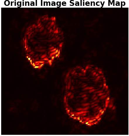
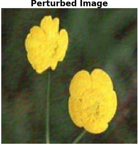
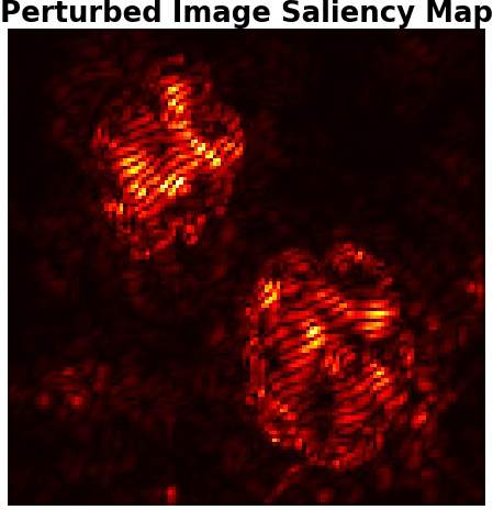
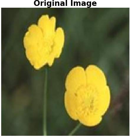
C.6 Additional Visualization Results

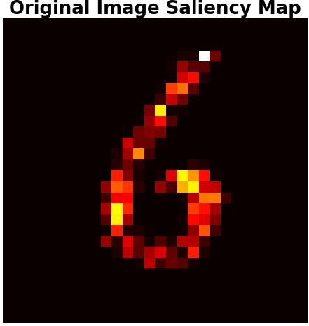
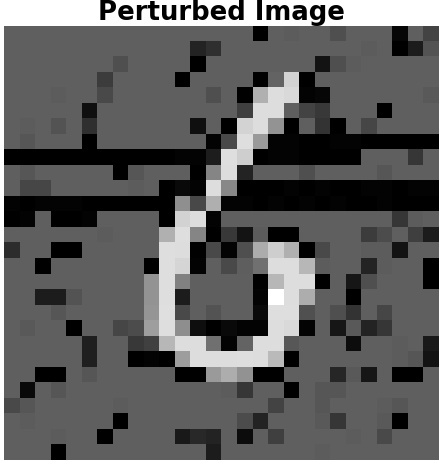
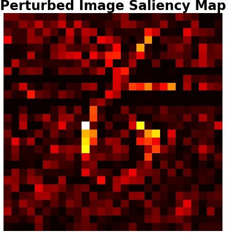
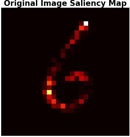
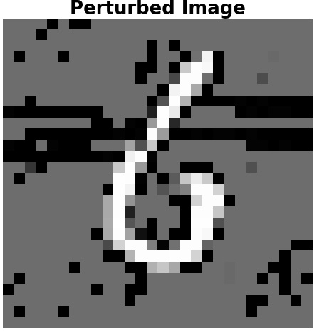
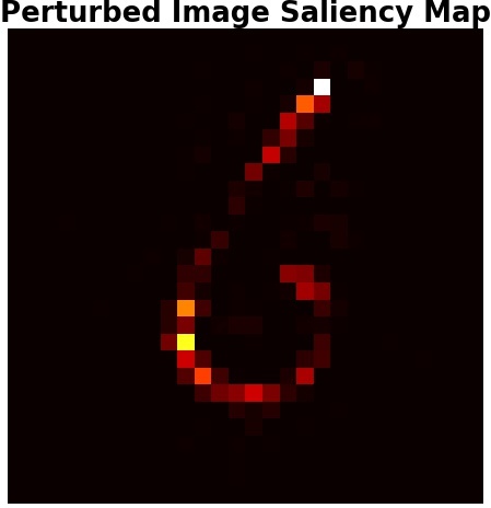
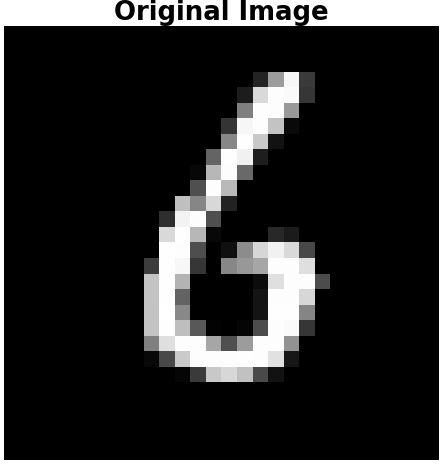
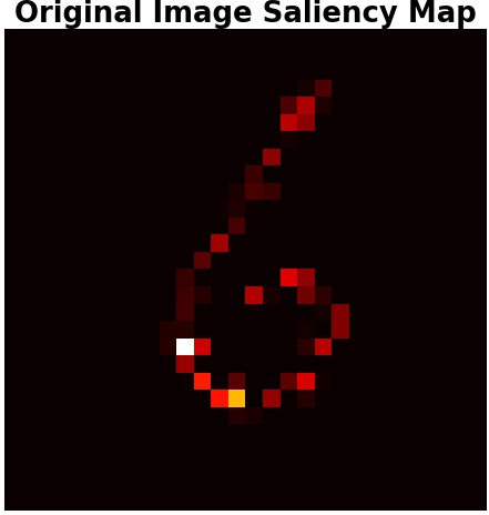
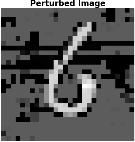
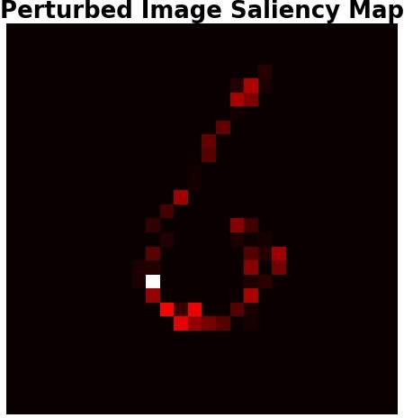
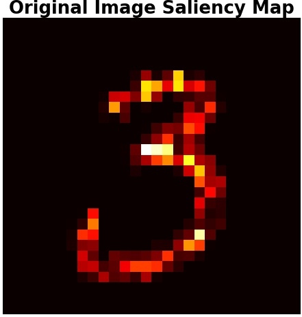
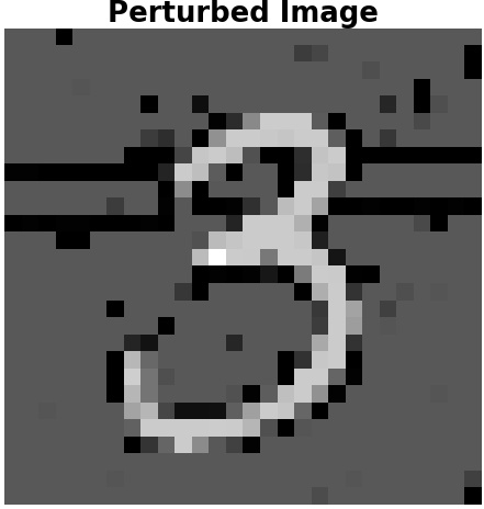
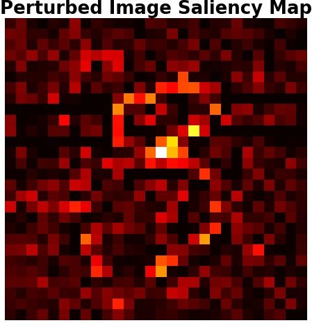
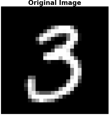
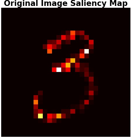
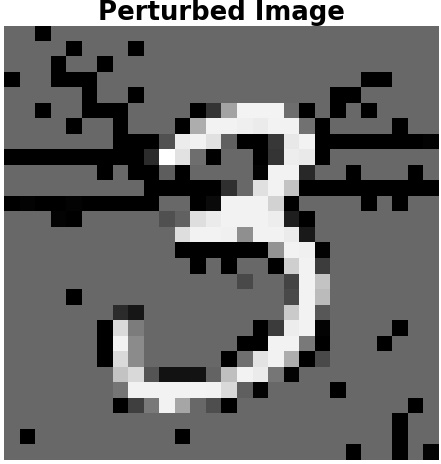
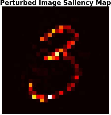
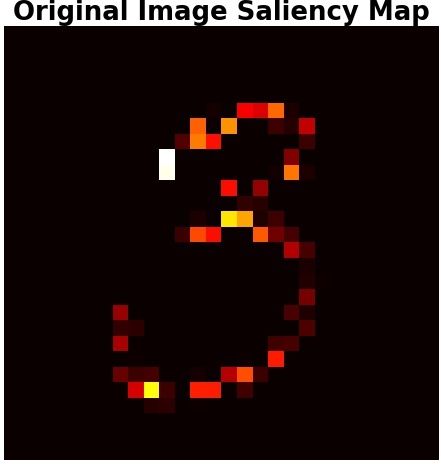
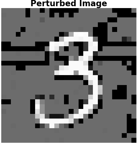
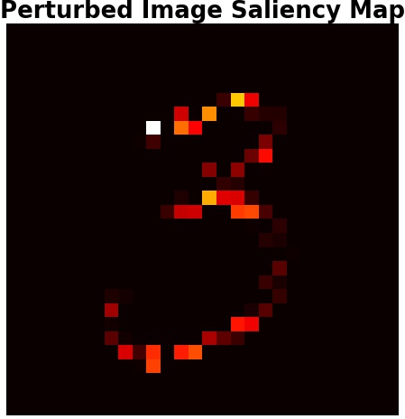
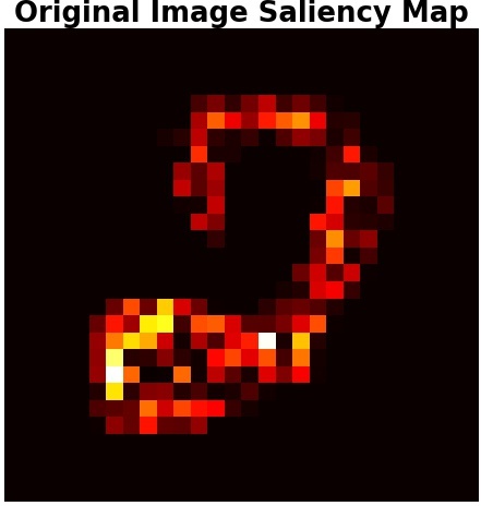
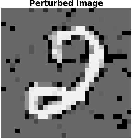
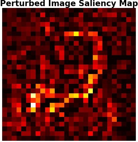
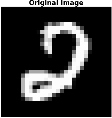
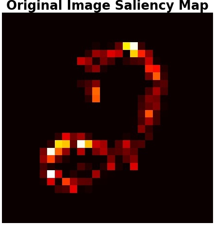
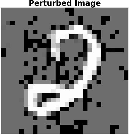
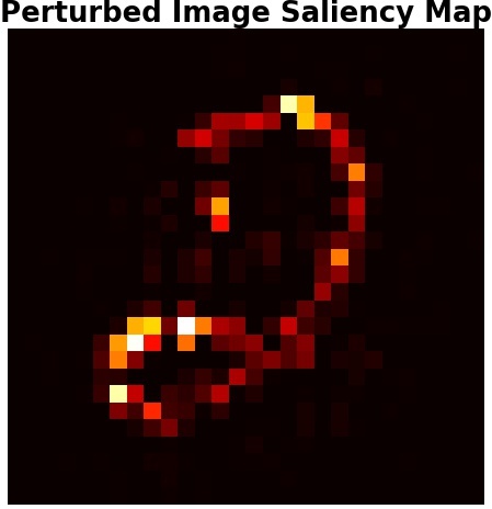
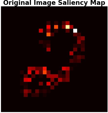
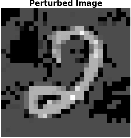
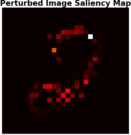
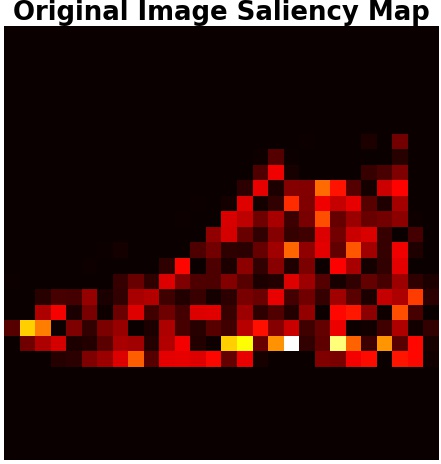
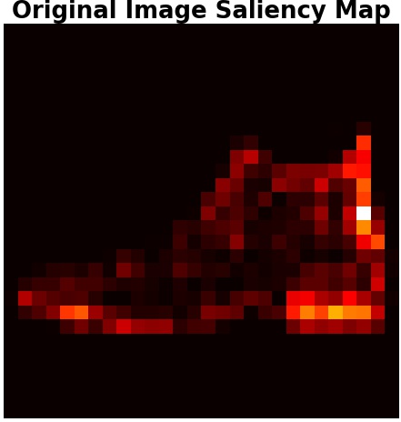
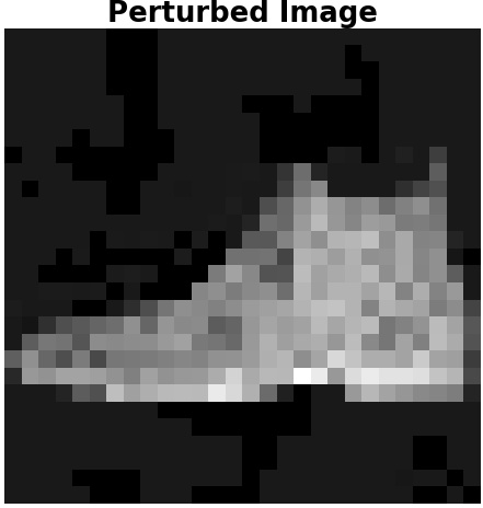
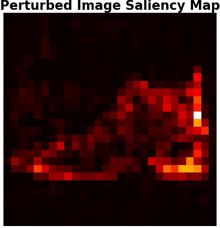
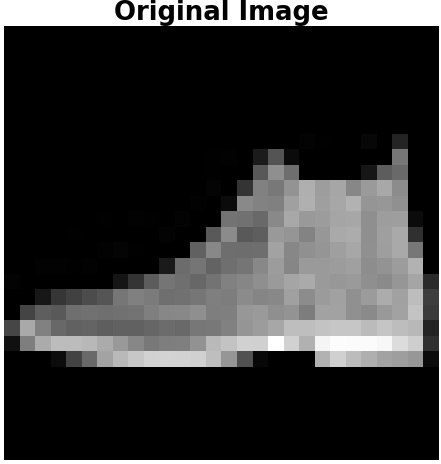
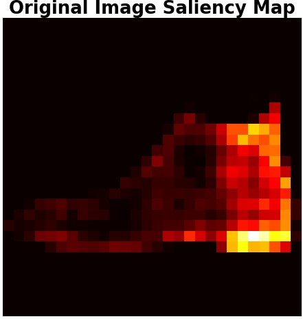
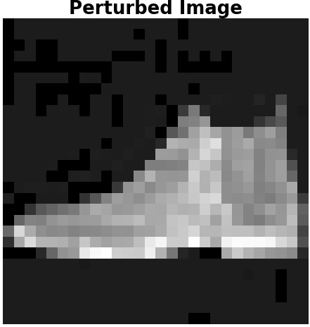
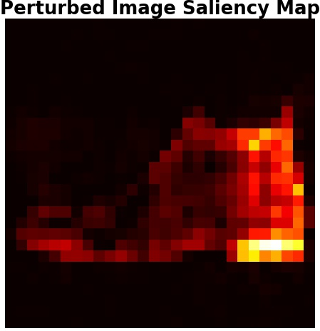
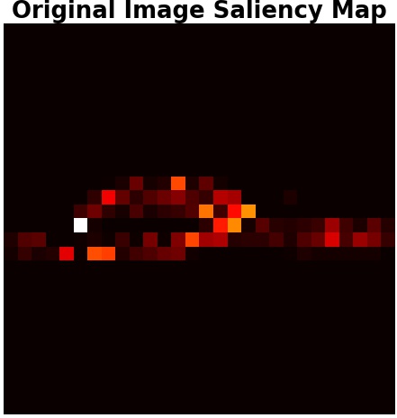
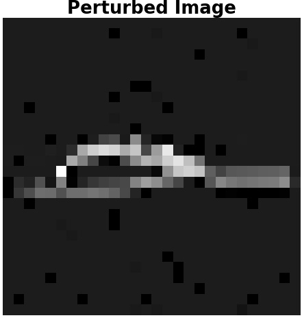
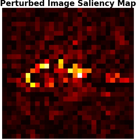
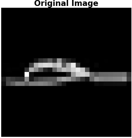
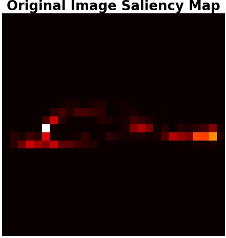
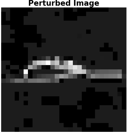
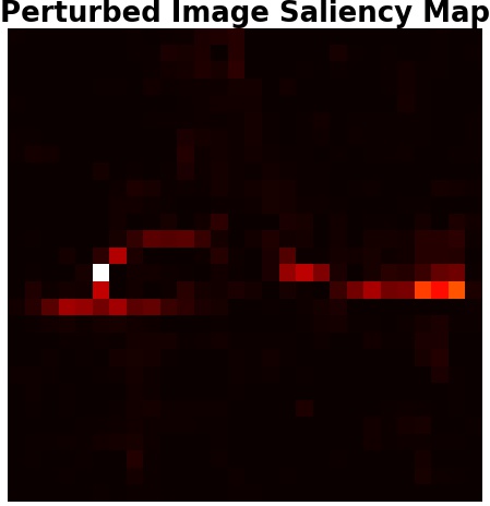
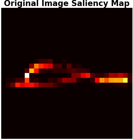
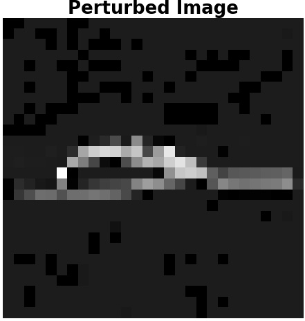
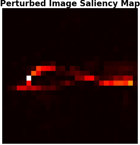
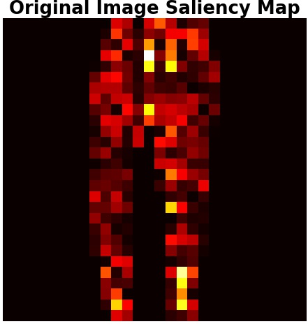
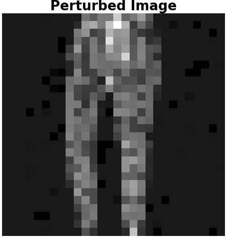
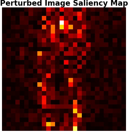
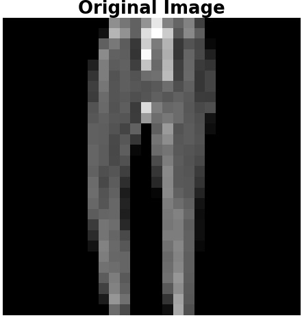
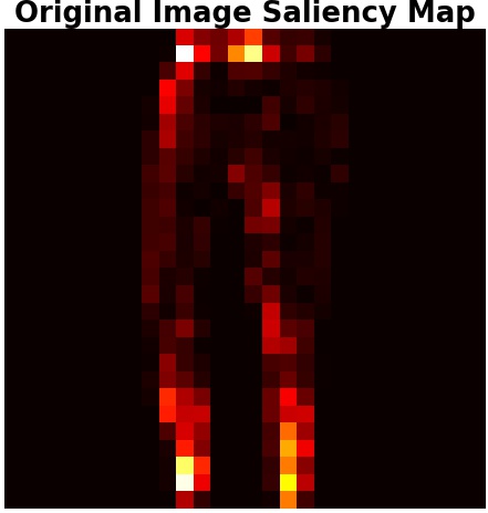
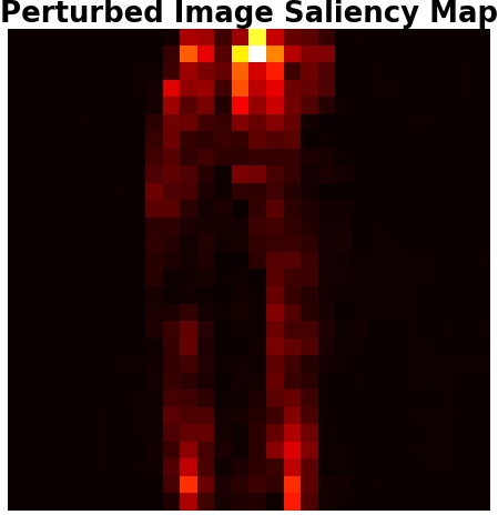
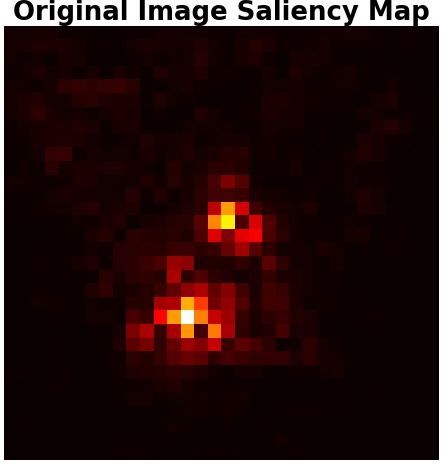
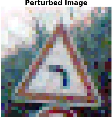
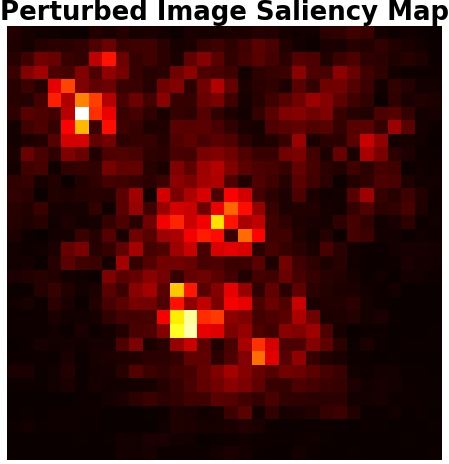
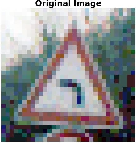
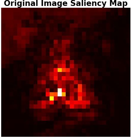
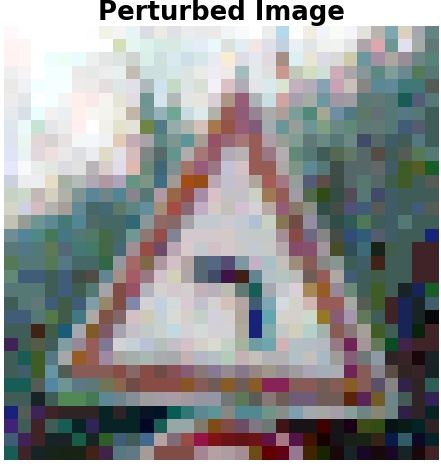
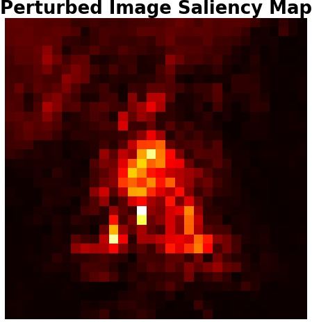
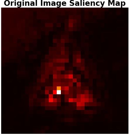
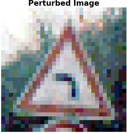
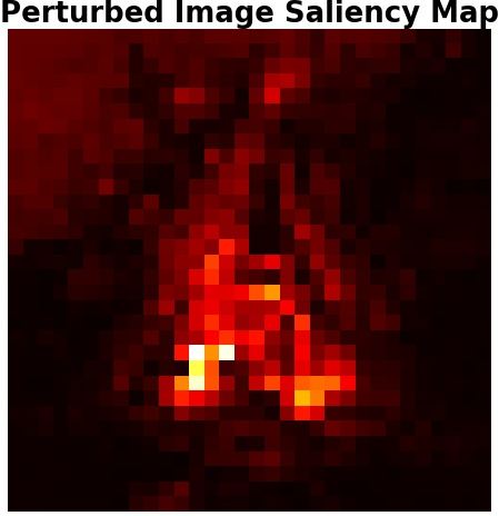
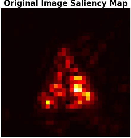
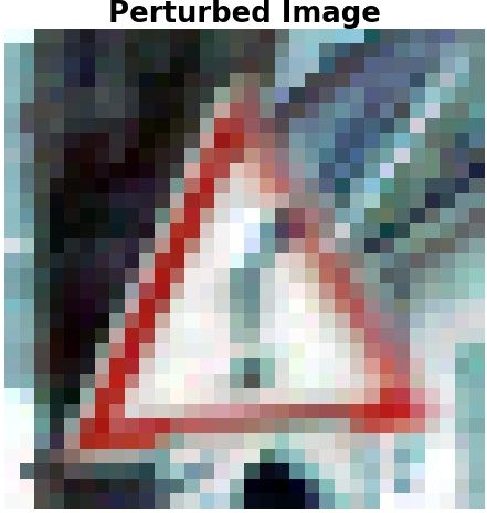
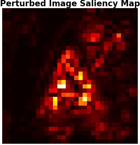
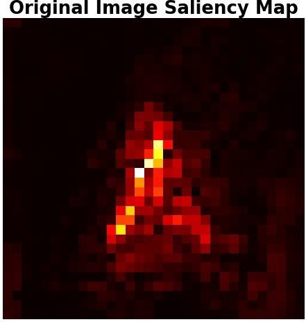
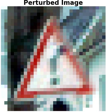
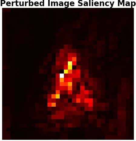
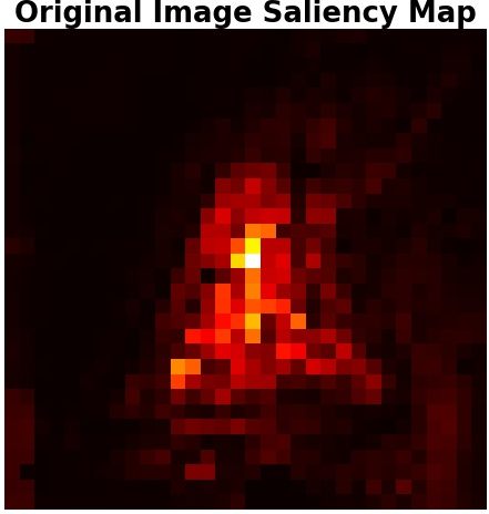
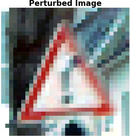
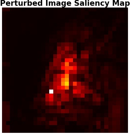
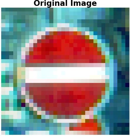
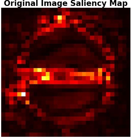
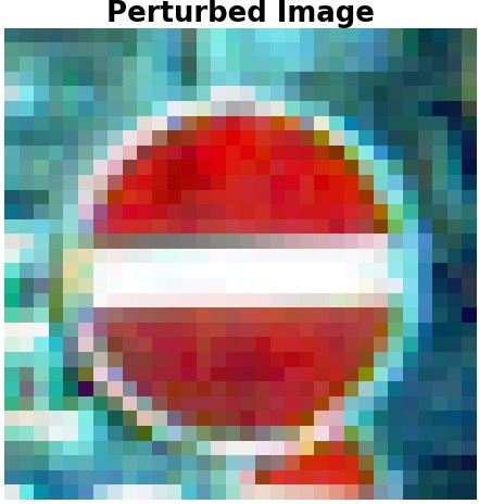
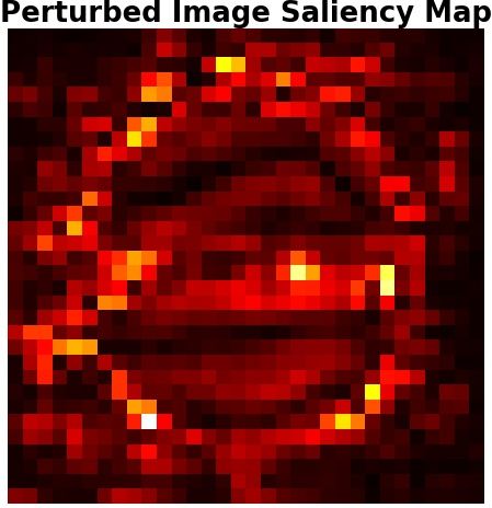
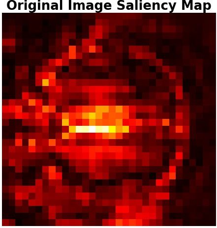
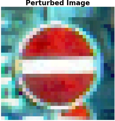
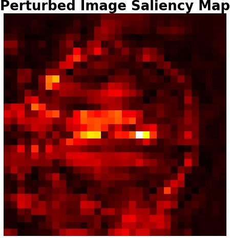
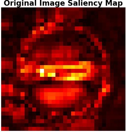
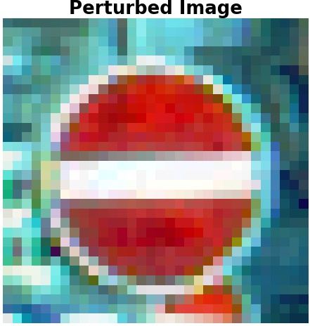
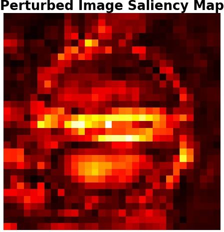
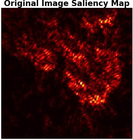
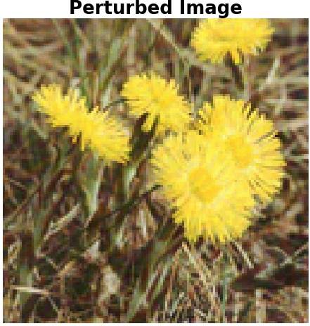
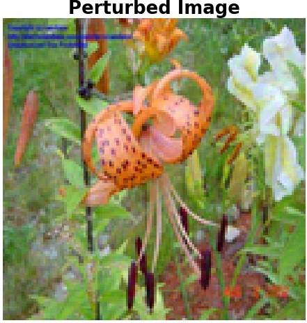
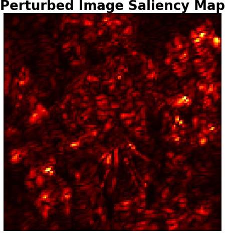
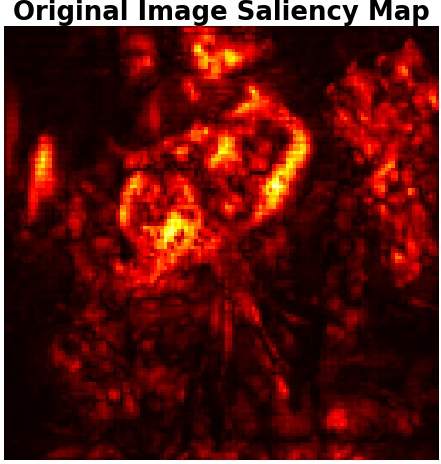
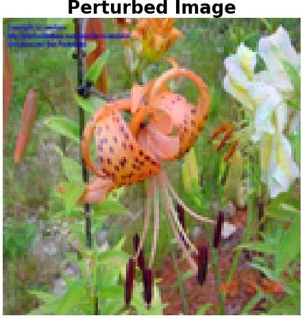
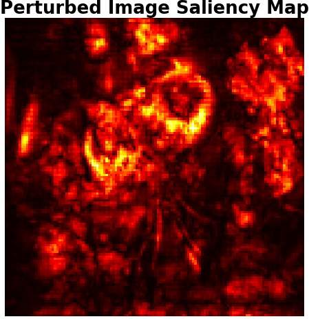
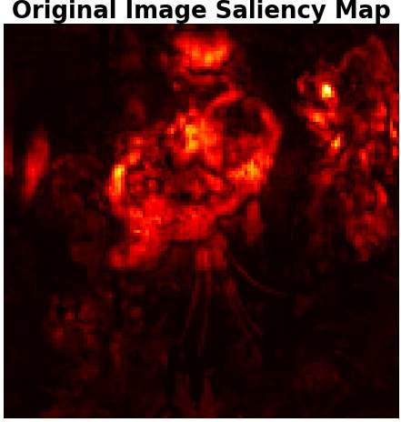
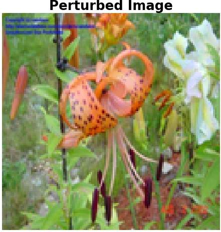
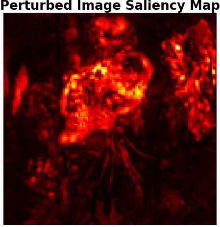
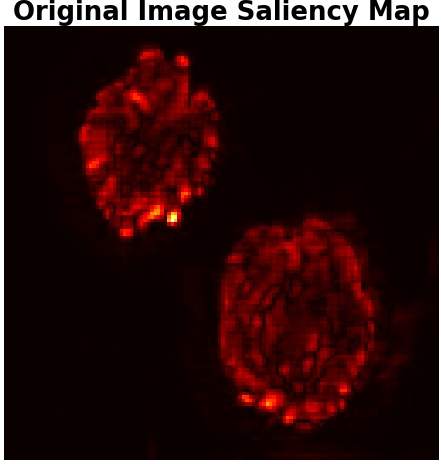
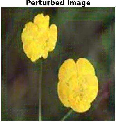
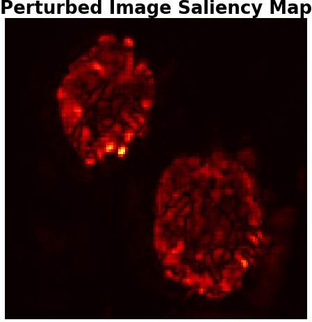
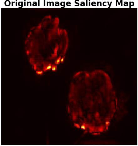
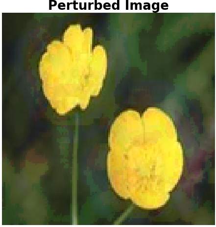
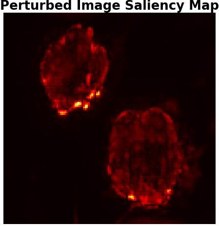
Here we provide more visualization results for MNIST in Figure 4, for Fashion-MNIST in Figure 6, for GTSRB in Figure 8, and for Flower in Figure 10.

NATURAL                        IG-NORM                        IG-SUM-NORM

Top-100 Intersection: 37.0%
Kendall’s Correlation: 0.0567

Top-100 Intersection: 64.0%
Kendall’s Correlation: 0.1823

Top-100 Intersection: 67.0%
Kendall’s Correlation: 0.2180

(a) For all images, the models give correct prediction – 6.

Top-100 Intersection: 43.0%
Kendall’s Correlation: 0.0563

Top-100 Intersection: 74.0%
Kendall’s Correlation: 0.1718

Top-100 Intersection: 84.0%
Kendall’s Correlation: 0.2501

(b) For all images, the models give correct prediction – 3.

Top-100 Intersection: 41.0%
Kendall’s Correlation: 0.1065

Top-100 Intersection: 83.0%
Kendall’s Correlation: 0.2837

Top-100 Intersection: 84.0%
Kendall’s Correlation: 0.3151

(c) For all images, the models give correct prediction – 2.

Figure 4: Top-100 and Kendall’s Correlation are rank correlations between original and perturbed saliency maps. NATURAL is the naturally trained model, IG-NORM and IG-SUM-NORM are models trained using our robust attribution method. We use attribution attacks described in [GAZ17] to perturb the attributions while keeping predictions intact. For all images, the models give correct predictions. However, the saliency maps (also called feature importance maps), computed via IG, show that attributions of the naturally trained model are very fragile, either visually or quantitatively as measured by correlation analysis, while models trained using our method are much more robust in their attributions.

NATURAL                        IG-NORM                        IG-SUM-NORM

Top-100 Intersection: 50.0%
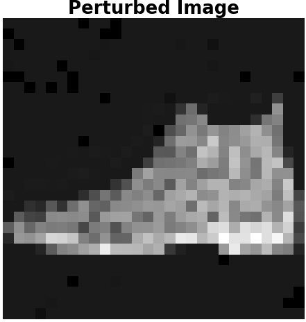
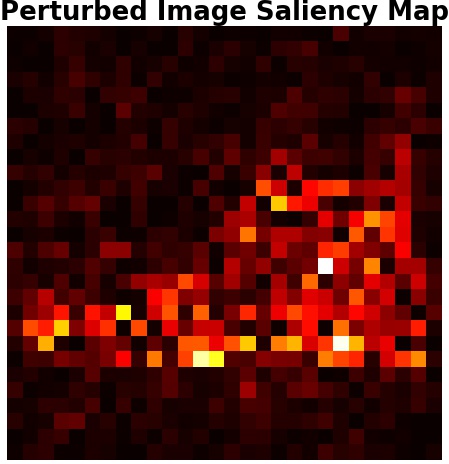
Kendall’s Correlation: 0.4595

Top-100 Intersection: 63.0%
Kendall’s Correlation: 0.6099

Top-100 Intersection: 87.0%
Kendall’s Correlation: 0.6607

(a) For all images, the models give correct prediction – Ankle boot.

Top-100 Intersection: 47.0%
Kendall’s Correlation: 0.1293

Top-100 Intersection: 54.0%
Kendall’s Correlation: 0.2508

Top-100 Intersection: 65.0%
Kendall’s Correlation: 0.3136

(b) For all images, the models give correct prediction – Sandal.

Top-100 Intersection: 39.0%
Kendall’s Correlation: 0.4129

Top-100 Intersection: 61.0%
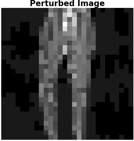
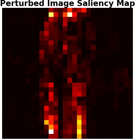
Kendall’s Correlation: 0.5983

Top-100 Intersection: 71.0%
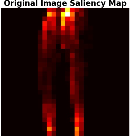
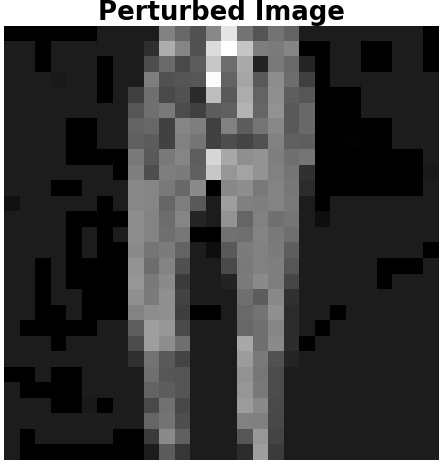
Kendall’s Correlation: 0.6699

(c) For all images, the models give correct prediction – Trouser.

Figure 6: Top-100 and Kendall’s Correlation are rank correlations between original and perturbed saliency maps. NATURAL is the naturally trained model, IG-NORM and IG-SUM-NORM are models trained using our robust attribution method. We use attribution attacks described in [GAZ17] to perturb the attributions while keeping predictions intact. For all images, the models give correct predictions. However, the saliency maps (also called feature importance maps), computed via IG, show that attributions of the naturally trained model are very fragile, either visually or quantitatively as measured by correlation analysis, while models trained using our method are much more robust in their attributions.

NATURAL                        IG-NORM                        IG-SUM-NORM

Top-100 Intersection: 45.0%
Kendall’s Correlation: 0.5822

Top-100 Intersection: 78.0%
Kendall’s Correlation: 0.7471

Top-100 Intersection: 80.0%
Kendall’s Correlation: 0.7886

(a) For all images, the models give correct prediction – Dangerous Curve to The Left.

Top-100 Intersection: 56.0%
Kendall’s Correlation: 0.6679

Top-100 Intersection: 85.0%
Kendall’s Correlation: 0.7963

Top-100 Intersection: 83.0%
Kendall’s Correlation: 0.8338

(b) For all images, the models give correct prediction – General Caution.

Top-100 Intersection: 43.0%
Kendall’s Correlation: 0.6160

Top-100 Intersection: 67.0%
Kendall’s Correlation: 0.7595

Top-100 Intersection: 81.0%
Kendall’s Correlation: 0.8128

(c) For all images, the models give correct prediction – No Entry.

Figure 8: Top-100 and Kendall’s Correlation are rank correlations between original and perturbed saliency maps. NATURAL is the naturally trained model, IG-NORM and IG-SUM-NORM are models trained using our robust attribution method. We use attribution attacks described in [GAZ17] to perturb the attributions while keeping predictions intact. For all images, the models give correct predictions. However, the saliency maps (also called feature importance maps), computed via IG, show that attributions of the naturally trained model are very fragile, either visually or quantitatively as measured by correlation analyses, while models trained using our method are much more robust in their attributions.

NATURAL                        IG-NORM                        IG-SUM-NORM

Top-1000 Intersection: 1.0%
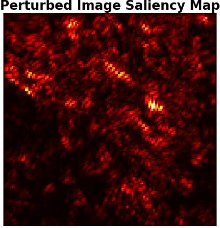
Kendall’s Correlation: 0.4601

Top-1000 Intersection: 65.4%
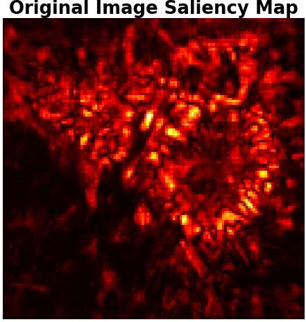
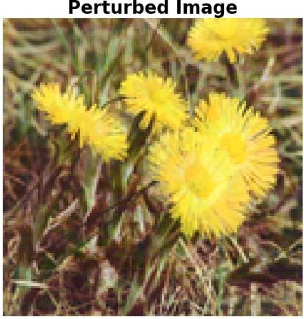
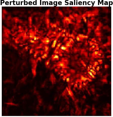
Kendall’s Correlation: 0.7248

Top-1000 Intersection: 63.9%
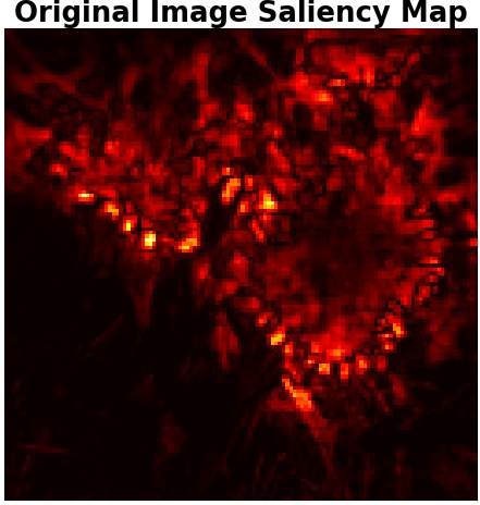
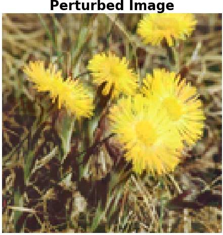
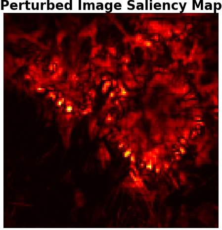
Kendall’s Correlation: 0.8036

(a) For all images, the models give correct prediction – Bluebell.

Top-1000 Intersection: 6.2%
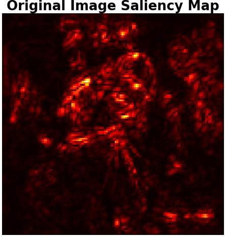
Kendall’s Correlation: 0.3863

Top-1000 Intersection: 58.20%
Kendall’s Correlation: 0.6694

Top-1000 Intersection: 65.9%
Kendall’s Correlation: 0.7970

(b) For all images, the models give correct prediction – Cowslip.

Top-1000 Intersection: 6.8%
Kendall’s Correlation: 0.4653

Top-1000 Intersection: 58.0%
Kendall’s Correlation: 0.7165

Top-1000 Intersection: 63.4%
Kendall’s Correlation: 0.8201

(c) For all images, the models give correct prediction – Tigerlily.

Figure 10: Top-1000 and Kendall’s Correlation are rank correlations between original and perturbed saliency maps. NATURAL is the naturally trained model, IG-NORM and IG-SUM-NORM are models trained using our robust attribution method. We use attribution attacks described in [GAZ17] to perturb the attributions while keeping predictions intact. For all images, the models give correct predictions. However, the saliency maps (also called feature importance maps), computed via IG, show that attributions of the naturally trained model are very fragile, either visually or quantitatively as measured by correlation analyses, while models trained using our method are much more robust in their attributions.

References

- [ABC+16] Martín Abadi, Paul Barham, Jianmin Chen, Zhifeng Chen, Andy Davis, Jeffrey Dean, Matthieu Devin, Sanjay Ghemawat, Geoffrey Irving, Michael Isard, et al. Tensorflow: A system for large-scale machine learning. In 12th USENIX Symposium on Operating Systems Design and Implementation (OSDI), pages 265–283, 2016.
- [BTEGN09] A. Ben-Tal, L. El Ghaoui, and A.S. Nemirovski. Robust Optimization. Princeton Series in Applied Mathematics. Princeton University Press, October 2009.
- [DL92] Harris Drucker and Yann LeCun. Improving generalization performance using double backpropagation. IEEE Trans. Neural Networks, 3(6):991–997, 1992.
- [EIS+19] Logan Engstrom, Andrew Ilyas, Shibani Santurkar, Dimitris Tsipras, Brandon Tran, and Aleksander Madry. Adversarial robustness as a prior for learned representations. arXiv 1906.00945, 2019.
- [GAZ17] Amirata Ghorbani, Abubakar Abid, and James Y. Zou. Interpretation of neural networks is fragile. CoRR, abs/1710.10547, 2017.
- [HZRS16] Kaiming He, Xiangyu Zhang, Shaoqing Ren, and Jian Sun. Deep residual learning for image recognition. In Proceedings of the IEEE conference on computer vision and pattern recognition, pages 770–778, 2016.
- [Ken38] Maurice G Kendall. A new measure of rank correlation. Biometrika, 30(1/2):81–93, 1938.
- [KM18] Zico Kolter and Aleksander Madry. Adversarial robustness – theory and practice, 2018. https://adversarial-ml-tutorial.org/.
- [LCB98] Yann LeCun, Corinna Cortes, and Christopher J.C. Burges. The mnist database of handwritten digits, 1998. http://yann.lecun.com/exdb/mnist/.
- [Lue97] David G. Luenberger. Optimization by Vector Space Methods. John Wiley & Sons, Inc., New York, NY, USA, 1st edition, 1997.
- [MEK15] Peyman Mohajerin Esfahani and Daniel Kuhn. Data-driven distributionally robust optimization using the wasserstein metric: performance guarantees and tractable reformulations. arXiv preprint arXiv:1505.05116, 2015.
- [MMS+17a] Aleksander Madry, Aleksandar Makelov, Ludwig Schmidt, Dimitris Tsipras, and Adrian Vladu. Towards deep learning models resistant to adversarial attacks. CoRR, abs/1706.06083, 2017.
- [MMS+17b] Aleksander Madry, Aleksandar Makelov, Ludwig Schmidt, Dimitris Tsipras, and Adrian Vladu. Towards deep learning models resistant to adversarial attacks. arXiv preprint arXiv:1706.06083, 2017.
- [NZ06] M-E Nilsback and Andrew Zisserman. A visual vocabulary for flower classification. In 2006 IEEE Computer Society Conference on Computer Vision and Pattern Recognition (CVPR’06), volume 2, pages 1447–1454. IEEE, 2006.
- [RD18] Andrew Slavin Ross and Finale Doshi-Velez. Improving the adversarial robustness and interpretability of deep neural networks by regularizing their input gradients. In Proceedings of the Thirty-Second AAAI Conference on Artificial Intelligence, (AAAI-18), pages 1660–1669, 2018.
- [RW09] R Tyrrell Rockafellar and Roger J-B Wets. Variational analysis, volume 317. Springer Science & Business Media, 2009.
- [SND18] Aman Sinha, Hongseok Namkoong, and John C. Duchi. Certifying some distributional robustness with principled adversarial training. In 6th International Conference on Learning Representations, ICLR 2018, 2018.
- [SSSI12] Johannes Stallkamp, Marc Schlipsing, Jan Salmen, and Christian Igel. Man vs. computer: Benchmarking machine learning algorithms for traffic sign recognition. Neural networks, 32:323–332, 2012.
- [STY17] Mukund Sundararajan, Ankur Taly, and Qiqi Yan. Axiomatic attribution for deep networks. In Proceedings of the 34th International Conference on Machine Learning, pages 3319–3328, 2017.
- [SVZ13] Karen Simonyan, Andrea Vedaldi, and Andrew Zisserman. Deep inside convolutional networks: Visualising image classification models and saliency maps. arXiv preprint arXiv:1312.6034, 2013.
- [TSE+19] Dimitris Tsipras, Shibani Santurkar, Logan Engstrom, Alexander Turner, and Aleksander Madry. Robustness may be at odds with accuracy. In International Conference on Learning Representations, 2019.
- [WK18] Eric Wong and J. Zico Kolter. Provable defenses against adversarial examples via the convex outer adversarial polytope. In Proceedings of the 35th International Conference on Machine Learning, ICML 2018, pages 5283–5292, 2018.
- [XRV17] Han Xiao, Kashif Rasul, and Roland Vollgraf. Fashion-mnist: a novel image dataset for benchmarking machine learning algorithms. arXiv preprint arXiv:1708.07747, 2017.