Abstract

We provide theoretical complexity analysis for new algorithms to compute the optimal transport (OT) distance between two discrete probability distributions, and demonstrate their favorable practical performance compared to state-of-art primal-dual algorithms. First, we introduce the accelerated primal-dual randomized coordinate descent (APDRCD) algorithm for computing the OT distance. We show that its complexity is $\widetilde{\mathcal{O}}(\frac{n^{5/2}}{\varepsilon})$, where $n$ stands for the number of atoms of these probability measures and $\varepsilon>0$ is the desired accuracy. This complexity bound matches the best known complexities of primal-dual algorithms for the OT problems, including the adaptive primal-dual accelerated gradient descent (APDAGD) and the adaptive primal-dual accelerated mirror descent (APDAMD) algorithms. Then, we demonstrate the improved practical efficiency of the APDRCD algorithm through comparative experimental studies. We also propose a greedy version of APDRCD, which we refer to as accelerated primal-dual greedy coordinate descent (APDGCD), to further enhance practical performance. Finally, we generalize the APDRCD and APDGCD algorithms to distributed algorithms for computing the Wasserstein barycenter for multiple probability distributions.

1 Introduction

Optimal transport has become an important topic in statistical machine learning. It finds the minimal cost couplings between pairs of probability measures and provides a geometrically faithful way to compare two probability distributions, with diverse applications in areas including Bayesian nonparametrics (Nguyen, 2013, 2016), scalable Bayesian inference (Srivastava et al., 2015, 2018), topic modeling (Lin et al., 2018), isotonic regression (Rigollet and Weed, 2019), and deep learning (Courty et al., 2017; Arjovsky et al., 2017; Tolstikhin et al., 2018).

Nevertheless, the practical impact of OT has been limited by its computational burden. By viewing the optimal transport distance as a linear programming problem, interior-point methods have been employed as a computational solver, with a best known practical complexity of $\widetilde{\mathcal{O}}(n^{3})$  (Pele and Werman, 2009). Recently, Lee and Sidford (Lee and Sidford, 2014) proposed to use the Laplace linear system solver to theoretically improve the complexity of interior-point methods to $\widetilde{\mathcal{O}}(n^{5/2})$. However, it remains a practical challenge to develop efficient interior-point implementations in the high-dimensional settings for OT applications in machine learning.

Several algorithms have been proposed to circumvent the scalability issue of the interior-point methods, including the Sinkhorn algorithm (Sinkhorn, 1974; Knight, 2008; Kalantari et al., 2008; Cuturi, 2013), which has a complexity bound of $\widetilde{\mathcal{O}}(\frac{n^{2}}{\varepsilon^{2}})$ where $\varepsilon>0$ is the desired accuracy (Dvurechensky et al., 2018). The Greenkhorn algorithm (Altschuler et al., 2017) further improves the performance of the Sinkhorn algorithm, with a theoretical complexity of $\widetilde{\mathcal{O}}(\frac{n^{2}}{\varepsilon^{2}})$ (Lin et al., 2019). However, for large-scale applications of the OT problem, particularly in randomized and asynchronous scenarios such as computational Wasserstein barycenters, existing literature has shown that neither the Sinkhorn algorithm nor the Greenkhorn algorithm are sufficiently scalable and flexible (Cuturi and Doucet, 2014; Dvurechenskii et al., 2018).

Recent research has demonstrated the advantages of the family of accelerated primal-dual algorithms over the Sinkhorn algorithms. This family includes the adaptive primal-dual accelerated gradient descent (APDAGD) algorithm (Dvurechensky et al., 2018) and the adaptive primal-dual accelerated mirror descent (APDAMD) algorithms (Lin et al., 2019), with complexity bounds of $\widetilde{\mathcal{O}}(\frac{n^{2.5}}{\varepsilon})$ and $\widetilde{\mathcal{O}}(\frac{n^{2}\sqrt{\gamma}}{\varepsilon})$, respectively, where $\gamma\leq\sqrt{n}$ is the inverse of the strong complexity constant of Bregman divergence with respect to the $l_{\infty}$-norm. In addition, the primal-dual algorithms possess the requisite flexibility and scalability compared to the Sinkhorn algorithm, which is crucial for computational OT problems in large-scale applications (Cuturi and Doucet, 2014; Ho et al., 2019). Specifically, they are flexible enough to be generalized to the computation of the Wasserstein barycenter for multiple probability distributions in decentralized and asynchronous settings (Cuturi and Doucet, 2014; Dvurechenskii et al., 2018).

In the optimization literature, primal-dual methods have served as standard techniques that are readily parallelized for high-dimensional applications (Combettes and Pesquet, 2012; Wainwright et al., 2005). On the other hand, coordinate descent methods have been shown to be well suited to the solution of large-scale machine learning problems (Nesterov, 2012; Richtárik and Takáč, 2016; Fercoq and Richtárik, 2015).

Our contributions. The contributions of the paper are three-fold.

1. We introduce an accelerated primal-dual randomized coordinate descent (APDRCD) algorithm for solving the OT problem. We provide a complexity upper bound of $\widetilde{\mathcal{O}}(\frac{n^{5/2}}{\varepsilon})$ for the APDRCD algorithm, which is comparable to the complexity of state-of-art primal-dual algorithms for OT problems, such as the APDAGD and APDAMD algorithms (Dvurechensky et al., 2018; Lin et al., 2019). To the best of our knowledge, this is the first accelerated primal-dual coordinate descent algorithm for computing the OT problem.

2. We show that the APDRCD algorithm outperforms the APDAGD and APDAMD algorithms with experiments on both synthetic and real image datasets. To further improve the practical performance of the APDRCD algorithm, we present a greedy version of it which we refer to as the accelerated primal-dual greedy coordinate descent (APDGCD) algorithm. To the best of our knowledge, the APDRCD and APDGCD algorithms achieve the best performance among state-of-art accelerated primal-dual algorithms on solving the OT problem.

3. We demonstrate that the APDRCD and APDGCD algorithms are suitable and parallelizable for other large-scale problems besides the OT problem, e.g., approximating the Wasserstein barycenter for a finite set of probability measures stored over a distributed network.

Organization. The remainder of the paper is organized as follows. In Section 2, we provide the formulation of the entropic OT problem and its dual form. In Section 3, we introduce the APDRCD algorithm for solving the regularized OT problem and provide a complexity upper bound for it. We then present the greedy APDGCD algorithm. In Section 4, we present comparative experiments between the APDRCD, the APDGCD algorithms and other primal-dual algorithms including the APDAGD and APDAMD algorithms. We conclude the paper with a few future directions in Section 5. Finally, the proofs of all the results are included in the Appendix A, and the generalized APDRCD and APDGCD algorithms for approximating Wasserstein barycenters are presented in Appendix B. Additional experiments are presented in Appendix C.

Notation. We denote the probability simplex $\Delta^{n}:=\{u=\left(u_{1},\ldots,u_{n}\right)\in\mathbb{R}^{n}:\sum_{i=1}^{n}u_{i}=1,\ u\geq 0\}$ for $n\geq 2$. Furthermore, $[n]$ stands for the set $\{1,2,\ldots,n\}$ while $\mathbb{R}^{n}_{+}$ stands for the set of all vectors in $\mathbb{R}^{n}$ with nonnegative components for any $n\geq 1$. For a vector $x\in\mathbb{R}^{n}$ and $1\leq p\leq\infty$, we denote $\|x\|_{p}$ as its $\ell_{p}$-norm and $\text{diag}(x)$ as the diagonal matrix with $x$ on the diagonal. For a matrix $A\in\mathbb{R}^{n\times n}$, the notation $\text{vec}(A)$ stands for the vector in $\mathbb{R}^{n^{2}}$ obtained from concatenating the rows and columns of $A$. 1 stands for a vector with all of its components equal to $1$. $\partial_{x}f$ refers to a partial gradient of $f$ with respect to $x$. Lastly, given the dimension $n$ and accuracy $\varepsilon$, the notation $a=\mathcal{O}\left(b(n,\varepsilon)\right)$ stands for the upper bound $a\leq C\cdot b(n,\varepsilon)$ where $C$ is independent of $n$ and $\varepsilon$. Similarly, the notation $a=\widetilde{\mathcal{O}}(b(n,\varepsilon))$ indicates the previous inequality may depend on the logarithmic function of $n$ and $\varepsilon$, and where $C>0$.

2 Problem Setup

In this section, we provide necessary background for the entropic regularized OT problem. The objective function for the problem is presented in Section 2.1 while its dual form as well as the key properties of that dual form are given in Section 2.2.

2.1 Entropic Regularized OT

As shown in (Kantorovich, 1942), the problem of approximating the OT distance between two discrete probability distributions with at most $n$ components is equivalent to the following linear programming problem:

$$\min\limits_{X\in\mathbb{R}^{n\times n}}\left\langle C,X\right\rangle$$ (1)

$$\ \ \ \textnormal{s.t.}\ \ X\textbf{1}=r,\ X^{\top}\textbf{1}=l,\ X\geq 0$$

where $X$ is a transportation plan, $C=(C_{ij})\in\mathbb{R}_{+}^{n\times n}$ is a cost matrix with non negative elements, and $r$ and $l$ refer to two known probability distributions in the probability simplex $\Delta^{n}$. The best known practical complexity bound for (1) is $\widetilde{\mathcal{O}}(n^{3})$ (Pele and Werman, 2009), while the best theoretical complexity bound is $\widetilde{\mathcal{O}}(n^{2.5})$ (Lee and Sidford, 2014), achieved via interior-point methods. However, these methods are not efficient in the high-dimensional setting of OT applications in machine learning. This motivates the entropic regularized OT problem (Cuturi, 2013):

$$\min\limits_{X\in\mathbb{R}_{+}^{n\times n}}\left\langle C,X\right\rangle-\eta H(X)$$ (2)

$$\ \ \ \textnormal{s.t.}\ \ X\textbf{1}=r,\ X^{\top}\textbf{1}=l,$$

where $\eta>0$ is the regularization parameter and $H(X)$ is the entropic regularization given by $H(X)\ :=\ -\sum_{i,j=1}^{n}X_{ij}\log(X_{ij})$. The main focus of the paper is to determine an $\varepsilon$-approximate transportation plan $\hat{X}\in\mathbb{R}_{+}^{n\times n}$ such that $\hat{X}\textbf{1}=r$ and $\hat{X}^{\top}\textbf{1}=l$ and the following bound holds:

$$\langle C,\hat{X}\rangle\ \leq\ \langle C,X^{*}\rangle+\varepsilon,$$ (3)

where $X^{*}$ is an optimal solution; i.e., an optimal transportation plan for the OT problem (1). To ease the ensuing presentation, we let $\langle C,\hat{X}\rangle$ denote an $\varepsilon$-approximation for the OT distance. Furthermore, we define matrix $A$ such that $A\text{vec}(X):=\begin{pmatrix}X\textbf{1}\\ X^{\top}\textbf{1}\end{pmatrix}$ for any $X\in\mathbb{R}^{n\times n}.$

2.2 Dual Entropic Regularized OT

The Lagrangian function for problem (2) is given by

$$\mathcal{L}(X,\alpha,\beta):= \left\langle C,X\right\rangle-\eta H(X)+\langle\alpha,r\rangle$$

$$+\langle\beta,l\rangle-\langle\alpha,X\textbf{1}\rangle-\langle\beta,X^{\top}\textbf{1}\rangle.$$

Given the Lagrangian function, the dual form of the entropic regularized OT problem can be obtained by solving the optimization problem $\min_{X\in\mathbb{R}^{n\times n}}\mathcal{L}(X,\alpha,\beta)$. Since the Lagrangian function $\mathcal{L}(\cdot,\alpha,\beta)$ is strictly convex, that optimization problem can be solved by setting $\partial_{X}\mathcal{L}(X,\alpha,\beta)=0$, which leads to the following form of the transportation plan: $X_{ij}\ =\ e^{\frac{-C_{ij}+\alpha_{i}+\beta_{j}}{\eta}-1}$ for all $i,j\in[n]$. With this solution, we have $\min_{X\in\mathbb{R}^{n\times n}}\mathcal{L}(X,\alpha,\beta)\ =\ -\eta\sum_{i,j=1}^{n}e^{-\frac{C_{ij}-\alpha_{i}-\beta_{j}}{\eta}-1}+\left\langle\alpha,r\right\rangle+\left\langle\beta,l\right\rangle$. The dual entropic regularized OT problem is, therefore, equivalent to the following optimization problem:

$$\min_{\alpha,\beta\in\mathbb{R}^{n}}\varphi(\alpha,\beta)$$

$$:=\eta\sum_{i,j=1}^{n}e^{-\frac{C_{ij}-\alpha_{i}-\beta_{j}}{\eta}-1}-\left\langle\alpha,r\right\rangle-\left\langle\beta,l\right\rangle$$ (4)

Building on Lemma 4.1 in (Lin et al., 2019), the dual objective function $\varphi(\alpha,\beta)$ can be shown to be smooth with respect to $\|\cdot\|_{2}$ norm:

Lemma 2.1.

The dual objective function $\varphi$ is smooth with respect to $\|.\|_{2}$ norm:

$$\varphi(\lambda_{1})-\varphi(\lambda_{2})-\left\langle\nabla\varphi(\lambda_{2}),\lambda_{1}-\lambda_{2}\right\rangle\leq\frac{2}{\eta}||\lambda_{1}-\lambda_{2}||^{2}_{2}.$$

Proof.

The proof is straightforward application of the result from Lemma 4.1 in (Lin et al., 2019). Here, we provide the details of this proof for the completeness. Indeed, invoking Lemma 4.1 in (Lin et al., 2019), we find that

$$\varphi(\lambda_{1})-\varphi(\lambda_{2})-\left\langle\nabla\varphi(\lambda_{2}),\lambda_{1}-\lambda_{2}\right\rangle\leq\frac{||A||_{1}^{2}}{2\eta}||\lambda_{1}-\lambda_{2}||^{2}_{\infty}.$$

Since $||A||_{1}$ is equal to the maximum $\ell_{1}$-norm of a column of A and each column of A contains only two nonzero elements which are equal to one, we have $||A||_{1}=2$. Combining with the fact that $||\lambda_{1}-\lambda_{2}||^{2}_{\infty}\leq||\lambda_{1}-\lambda_{2}||^{2}_{2}$, we establish the result. ∎

3 Accelerated Primal-Dual Coordinate Descent Algorithms

In this section, we present and analyze an accelerated primal-dual coordinate descent algorithms to obtain an $\varepsilon$-approximate transportation plan for the OT problem (1). First, in Section 3.1, we introduce the accelerated primal-dual randomized coordinate descent (APDRCD) method for the entropic regularized OT problem. Then, following the approximation scheme of (Altschuler et al., 2017), we show how to approximate the OT distance within the APDRCD algorithm; see Algorithm 2 for the pseudo-code for this problem. Furthermore, we provide theoretical analysis to establish a complexity bound of $\mathcal{O}(\frac{n^{\frac{5}{2}}\sqrt{||C||_{\infty}\log(n)}}{\varepsilon})$ for the APDRCD algorithm to achieve an $\varepsilon$-approximate transportation plan for the OT problem in Section 3.2. This complexity upper bound of the APDRCD algorithm matches the best known complexity bounds of the APDAGD (Dvurechensky et al., 2018) and APDAMD algorithms (Lin et al., 2019). Finally, to further improve the practical performance of the algorithm, we present a greedy variant—the accelerated primal-dual greedy coordinate descent (APDGCD) algorithm—in Section 3.3.

1 Input: $\{\theta_{i}|\theta_{0}=1,\frac{1-\theta_{i+1}}{\theta_{i+1}^{2}}=\frac{1}{\theta_{i}^{2}}\},C_{0}=1,\lambda^{0}=z^{0}=k=0,L=\frac{4}{\eta}$

2 while $||Ax^{k}-b||_{1}>\varepsilon^{\prime}$ do

3      Set $y^{k}=(1-\theta_{k})\lambda^{k}+\theta_{k}z^{k}$

4       Compute $x^{k}=\frac{1}{C_{k}}\biggr{(}\sum_{j=0}^{k}\dfrac{x(y^{j})}{\theta_{j}}\biggr{)}$

5       Randomly sample one coordinate $i_{k}$ where $i_{k}\in\{1,2,...,2n\}$:

6       Update

$$\lambda^{k+1}_{i_{k}}=y^{k}_{i_{k}}-\frac{1}{L}\nabla_{i_{k}}\varphi(y^{k})$$ (5)

7       Update

$$z^{k+1}_{i_{k}}=z^{k}_{i_{k}}-\frac{1}{2nL\theta_{k}}\nabla_{i_{k}}\varphi(y^{k})$$ (6)

8       Update $k=k+1$ and $C_{k}=C_{k}+\frac{1}{\theta_{k}}$

9 end while

Output: $X^{k}$ where $x^{k}=vec(X^{k})$

Algorithm 1 APDRCD ($C,\eta,A,b,\varepsilon^{\prime}$)

3.1 Accelerated Primal-Dual Randomized Coordinate Descent (APDRCD)

We denote by $L$ the Lipschitz constant for the dual objective function $\varphi$, which means that $L:=\frac{4}{\eta}$, and $x(\lambda):=\mathop{\arg\max}\limits_{x\in\mathbb{R}^{n\times n}}\biggr{\{}-\left\langle C,x\right\rangle-\left\langle A^{\top}\lambda,x\right\rangle\biggr{\}}$. The APDRCD algorithm is initialized with the auxiliary sequence $\{\theta_{i}\}$ and two auxiliary dual variable sequences $\{\lambda_{i}\}$ and $\{\mathbf{z}_{i}\}$, where the first auxiliary sequence $\{\theta_{k}\}$ is used for the key averaging step and the two dual variable sequences are used to perform the accelerated randomized coordinate descent on the dual objective function $\varphi$ as a subroutine. The APDRCD algorithm is composed of two main parts. First, exploiting the convexity property of the dual objective function, we perform a randomized accelerated coordinate descent step on the dual objective function as a subroutine in step 5 and 6. In the second part, we take a weighted average over the past iterations to get a good approximate solution for the primal problem from the approximate solutions to the dual problem (2.2). Notice that the auxiliary sequence $\{\theta_{k}\}$ is decreasing and the primal solutions corresponding to the more recent dual solutions have larger weight in this average.

  Input: $\eta=\dfrac{\varepsilon}{4\log(n)}$ and $\varepsilon^{\prime}=\dfrac{\varepsilon}{8\left\|C\right\|_{\infty}}$.

  Step 1: Let $\tilde{r}\in\Delta_{n}$ and $\tilde{l}\in\Delta_{n}$ be defined as

$$\left(\tilde{r},\tilde{l}\right)=\left(1-\frac{\varepsilon^{\prime}}{8}\right)\left(r,l\right)+\frac{\varepsilon^{\prime}}{8n}\left(\textbf{1},\textbf{1}\right).$$

  Step 2: Let $A\in\mathbb{R}^{2n\times n^{2}}$ and $b\in\mathbb{R}^{2n}$ be defined by

$$Avec(X)=\left(\begin{smallmatrix}X\bm{1}\\ X^{T}\bm{1}\end{smallmatrix}\right)\ \ \text{and}\ \ b=\left(\begin{smallmatrix}\tilde{r}\\ \tilde{l}\end{smallmatrix}\right)$$

  Step 3: Compute $\tilde{X}=\text{APDRCD}\left(C,\eta,A,b,\varepsilon^{\prime}/2\right)$ with $\varphi$ defined in 2.2.

  Step 4: Round $\tilde{X}$ to $\hat{X}$ by Algorithm 2 (Altschuler et al., 2017) such that $\hat{X}\textbf{1}=r$, $\hat{X}^{\top}\textbf{1}=l$.

  Output: $\hat{X}$.

Algorithm 2 Approximating OT by APDRCD

3.2 Complexity Analysis of APDRCD

Given the updates from APDRCD algorithm in Algorithm 1, we have the following result regarding the difference of the values of $\varphi$ at $\lambda^{k+1}$ and $y^{k}$:

Lemma 3.1.

Given the updates $\lambda^{k+1}$ and $y^{k}$ from the APDRCD algorithm, we have the following inequality:

$$\varphi(\lambda^{k+1})-\varphi(y^{k})\leq-\frac{1}{2L}|\nabla_{i_{k}}\varphi(y^{k})|^{2},$$

where $i_{k}$ is chosen in the APDRCD algorithm.

Proof.

For convenience, we define a vector-valued function $h(i_{k})\in\mathbb{R}^{2n}$ such that $h(i_{k})_{i}=1$ if $i=i_{k}$, and $h(i_{k})_{i}=0$ otherwise. By the update in Eq. (5) of Algorithm 1, we obtain:

$$\varphi(\lambda^{k+1})-\varphi(y^{k})=\varphi\biggr{(}y^{k}-h(i_{k})\cdot\frac{1}{L}\nabla_{i_{k}}\varphi(y^{k})\biggr{)}-\varphi(y^{k}).$$ (7)

Due to the smoothness of $\varphi$ with respect to $\|.\|_{2}$ norm in Lemma 2.1, the following inequalities hold:

$$\varphi\biggr{(}y^{k}-h(i_{k})\frac{1}{L}\nabla_{i_{k}}\varphi(y^{k})\biggr{)}-\varphi(y^{k})$$

$$\leq \left\langle\nabla\varphi(y^{k}),-h(i_{k})\frac{1}{L}\nabla_{i_{k}}\varphi(y^{k})\right\rangle$$

$$\ +\frac{L}{2}||h(i_{k})\frac{1}{L}(\nabla_{i_{k}}\varphi(y^{k}))||^{2}$$

$$= -\frac{1}{L}\left\langle\nabla\varphi(y^{k}),\nabla_{i_{k}}\varphi(y^{k})h(i_{k})\right\rangle+\frac{1}{2L}(\nabla_{i_{k}}\varphi(y^{k}))^{2}$$

$$= -\frac{1}{L}(\nabla_{i_{k}}\varphi(y^{k}))^{2}+\frac{1}{2L}(\nabla_{i_{k}}\varphi(y^{k}))^{2}$$

$$= -\frac{1}{2L}(\nabla_{i_{k}}\varphi(y^{k}))^{2}.$$ (8)

Combining the results of Eq. (7) and Eq. (3.2) completes the proof of the lemma. ∎

The result of Lemma 3.1 is vital for establishing an upper bound for $\mathbb{E}_{i_{k}}\varphi(\lambda^{k+1})$, as shown in the following lemma.

Lemma 3.2.

For each iteration ($k>0$) of the APDRCD algorithm, we have

$$\mathbb{E}_{i_{k}}\big{[}\varphi(\lambda^{k+1})\big{]}$$

$$\leq(1-\theta_{k})\varphi(\lambda^{k})+\theta_{k}\big{[}\varphi(y^{k})+(\lambda-y^{k})^{T}\nabla\varphi(y^{k})\big{]}$$

$$\ +2L^{2}n^{2}\theta_{k}^{2}\biggr{(}||\lambda-z^{k}||^{2}-\mathbb{E}_{i_{k}}\big{[}||\lambda-z^{k+1}||^{2}\big{]}\biggr{)},$$

where the outer expectation in the above display is taken with respect to the random coordinate $i_{k}$ in Algorithm 1.

The proof of Lemma 3.2 is in Appendix A.1. Now, equipped with the result of Lemma 3.2, we are ready to provide the convergence guarantee and complexity bound of the APDRCD algorithm for approximating the OT problem. First, we start with the following result regarding an upper bound on $k$ to reach the stopping rule $||A\text{vec}(X^{k})-b||_{1}\leq\varepsilon^{\prime}$ for $\varepsilon^{\prime}=\dfrac{\varepsilon}{8\left\|C\right\|_{\infty}}$. Here, the outer expectation is taken with respect to the random coordinates $i_{j}$ in Algorithm 1 for $1\leq j\leq k$.

Theorem 3.3.

The APDRCD algorithm for approximating optimal transport (Algorithm 2) returns an output $X^{k}$ that satisfies the stopping criterion $\mathbb{E}\big{[}||A\text{vec}(X^{k})-b||_{1}\bigr{]}\leq\varepsilon^{\prime}$ in a number of iterations k bounded as follows:

$$k\leq 12n^{\frac{3}{2}}\sqrt{\frac{R+1/2}{\varepsilon}}+1,$$

where $R:=\frac{||C||_{\infty}}{\eta}+\log(n)-2\log(\min\limits_{1\leq i,j\leq n}\{r_{i},l_{i}\})$. Here, $\varepsilon^{\prime}$ and $\eta$ are chosen in Algorithm 2.

The proof of Theorem 3.3 is provided in Appendix A.2. Given an upper bound on $k$ for the stopping rule in Theorem 3.3 where $\varepsilon^{\prime}=\dfrac{\varepsilon}{8\left\|C\right\|_{\infty}}$ in Theorem 3.3, we obtain the following complexity bound for the APDRCD algorithm.

Theorem 3.4.

The APDRCD algorithm for approximating optimal transport (Algorithm 2) returns $\hat{X}\in\mathbb{R}^{n\times n}$ satisfying $\hat{X}\textbf{1}=r$, $\hat{X}^{T}\textbf{1}=l$ and $\mathbb{E}[\langle C,\hat{X}\rangle]-\left\langle C,X^{\ast}\right\rangle\leq\epsilon$ in a total number of

$$\mathcal{O}\biggr{(}\frac{n^{\frac{5}{2}}\sqrt{||C||_{\infty}\log(n)}}{\varepsilon}\biggr{)}$$

arithmetic operations.

The proof of Theorem 3.4 is provided in Appendix A.3. We show in Appendix A.3 that Theorem 3.4 also directly implies a complexity bound for obtaining an $\epsilon$-optimal solution with high probability. Theorem 3.4 indicates that the complexity upper bound of APDRCD matches the best known complexity $\widetilde{\mathcal{O}}(\frac{n^{5/2}}{\varepsilon})$ of the APDAGD (Dvurechensky et al., 2018) and APDAMD (Lin et al., 2019) algorithms. Furthermore, that complexity of APDRCD is better than that of the Sinkhorn and Greenkhorn algorithms, which is $\widetilde{\mathcal{O}}(\frac{n^{2}}{\varepsilon^{2}})$, in terms of the desired accuracy $\varepsilon$. Later in Section 4, we demonstrate that the APDRCD algorithm also has better practical performance than APDAGD and APDAMD algorithms on both synthetic and real datasets.

1 Input: $\{\theta_{i}|\theta_{0}=1,\frac{1-\theta_{i+1}}{\theta_{i+1}^{2}}=\frac{1}{\theta_{i}^{2}}\},C_{0}=1,\lambda^{0}=z^{0}=k=0,L=\frac{4}{\eta}$

2 while $||Ax^{k}-b||_{1}>\varepsilon^{\prime}$ do

3      Set $y^{k}=(1-\theta_{k})\lambda^{k}+\theta_{k}z^{k}$

4       Compute $x^{k}=\frac{1}{C_{k}}\biggr{(}\sum_{j=0}^{k}\dfrac{x(y^{j})}{\theta_{j}}\biggr{)}$

5       Select coordinate $i_{k}=\mathop{\rm argmax}\limits_{i_{k}\in\{1,2,...,2n\}}|\nabla_{i_{k}}\varphi(y^{k})|$: Update

$$\lambda^{k+1}_{i_{k}}=y^{k}_{i_{k}}-\frac{1}{L}\nabla_{i_{k}}\varphi(y^{k})$$

Update

$$z^{k+1}_{i_{k}}=z^{k}_{i_{k}}-\frac{1}{2nL\theta_{k}}\nabla_{i_{k}}\varphi(y^{k})$$

Update $k=k+1$ and $C_{k}=C_{k}+\frac{1}{\theta_{k}}$

6 end while

Output: $X^{k}$ where $x^{k}=vec(X^{k})$

Algorithm 3 APDGCD ($C,\eta,A,b,\varepsilon^{\prime}$)

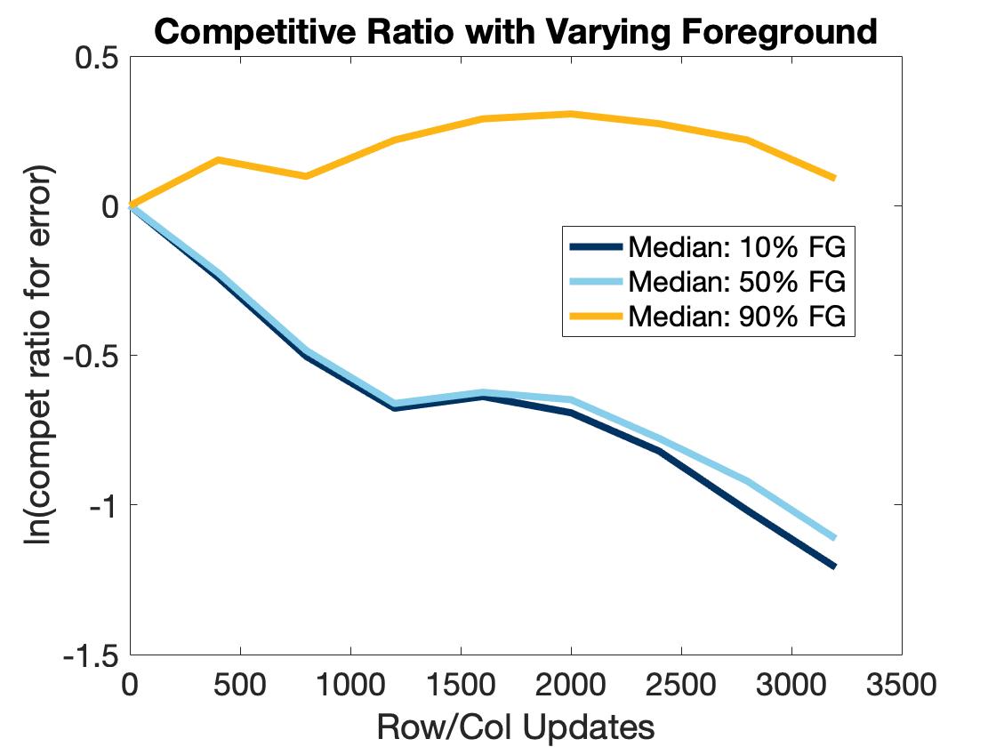
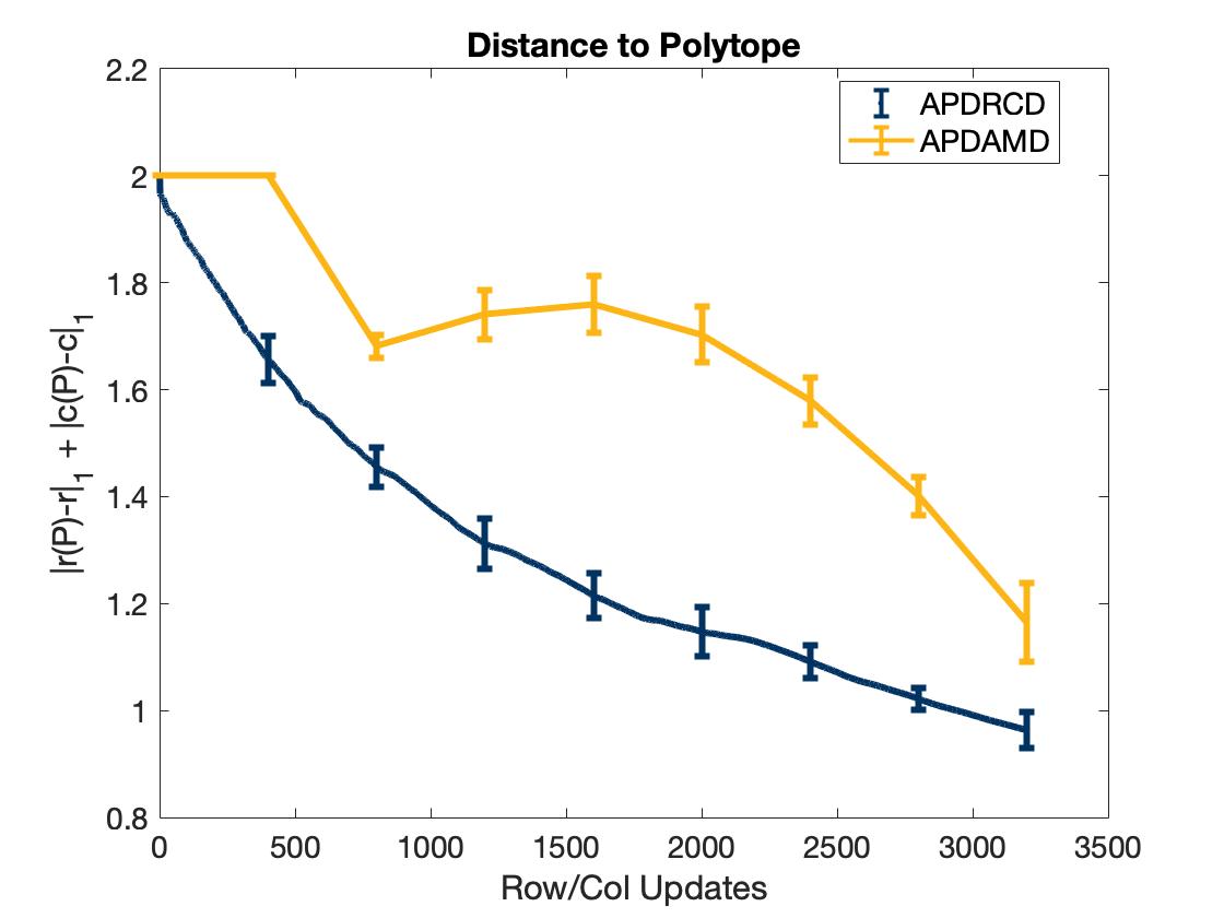
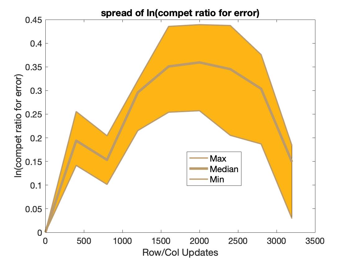
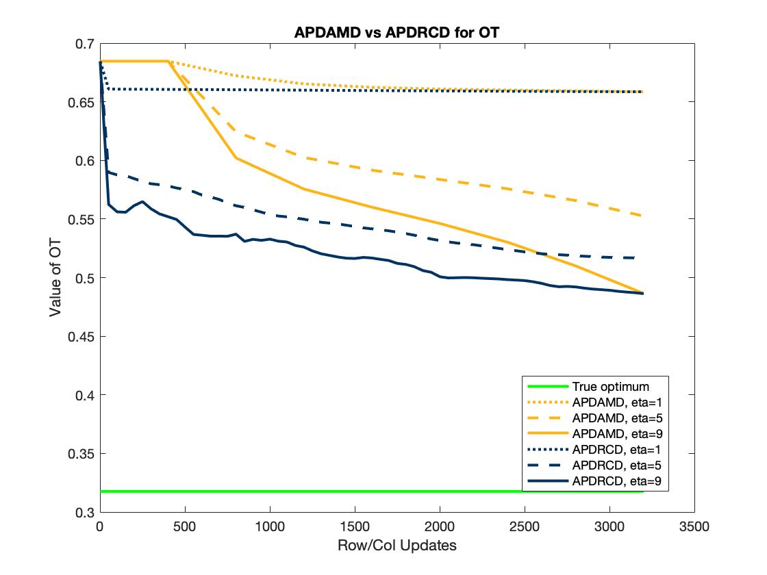
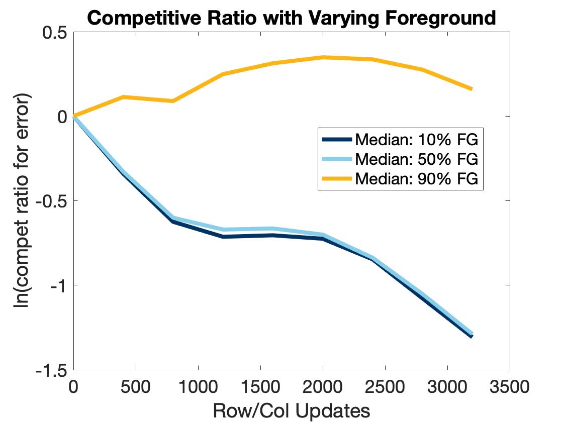
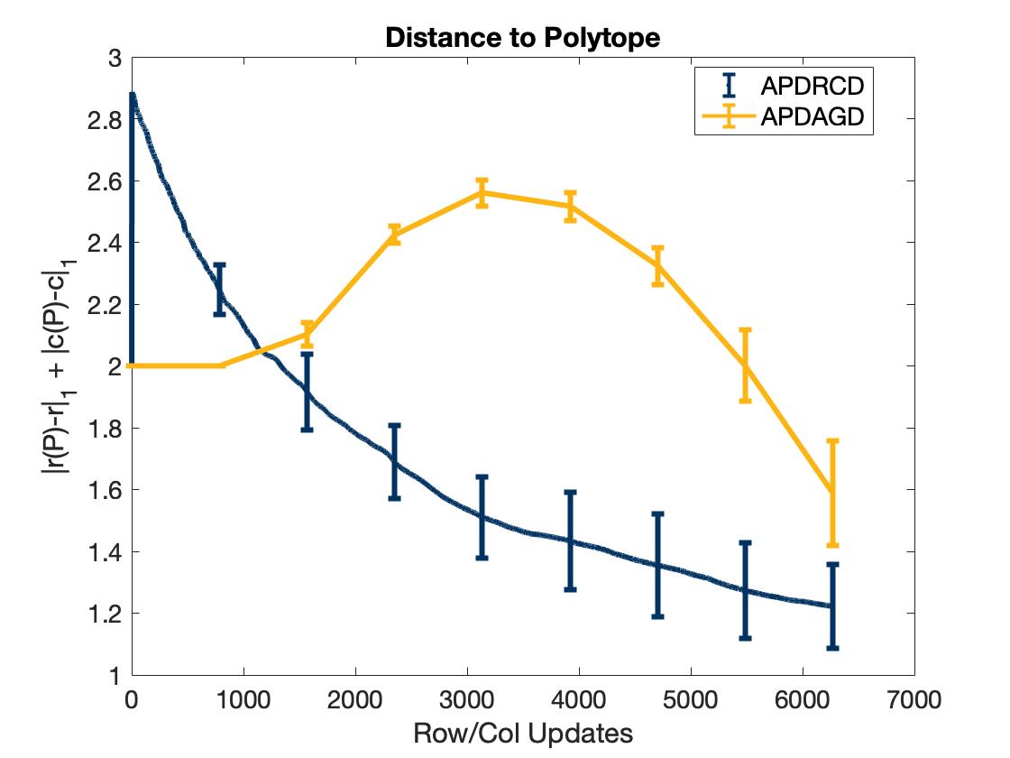
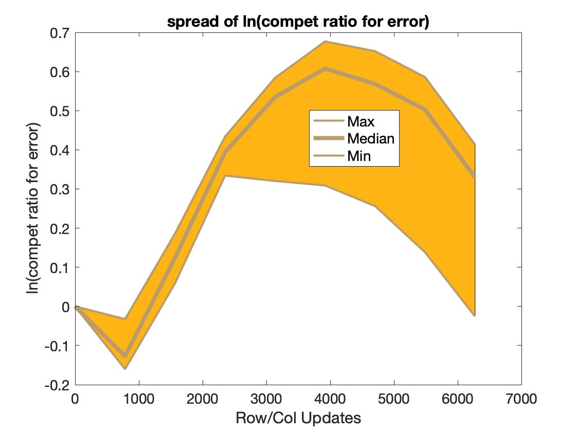
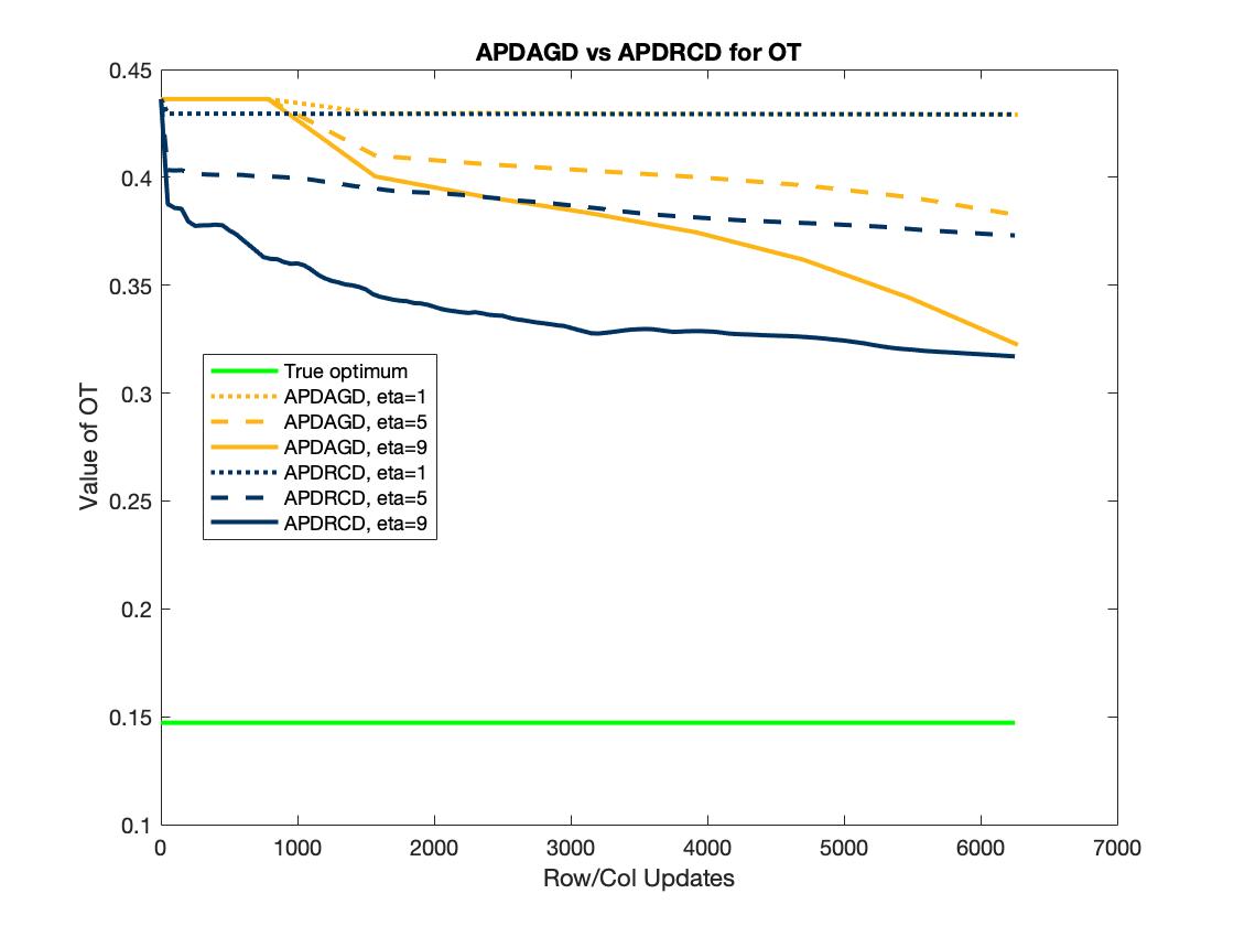
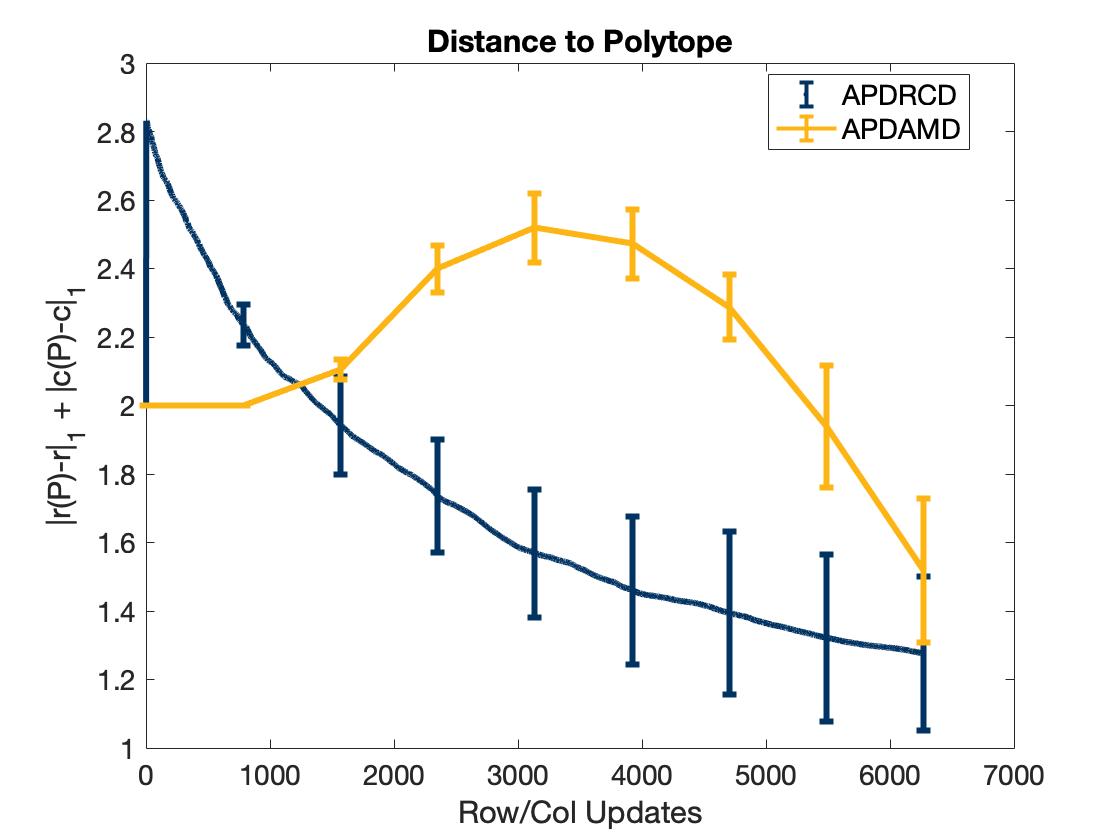
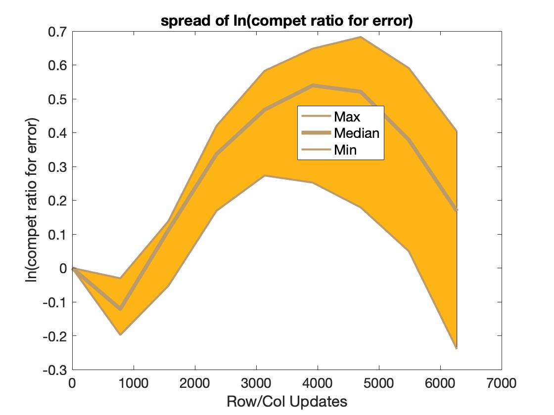
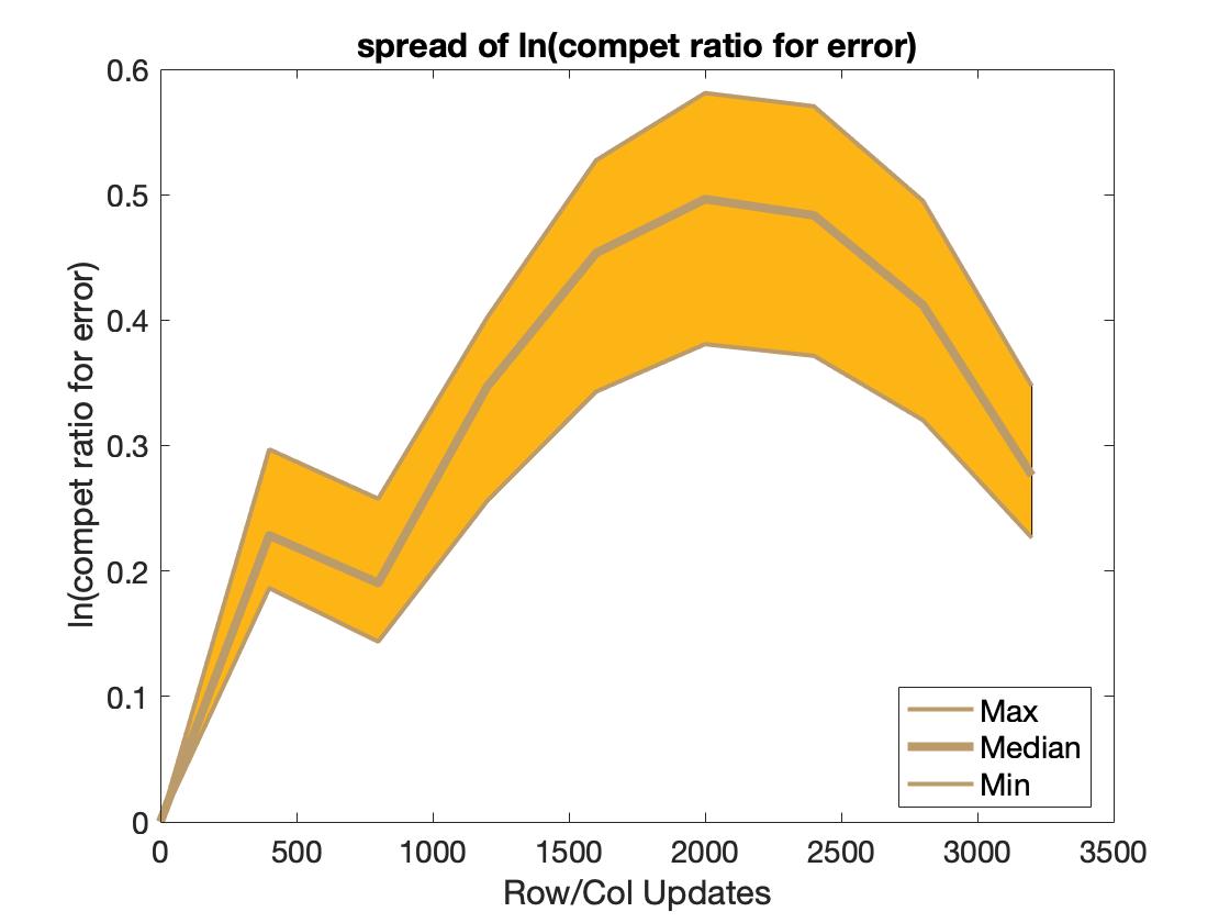
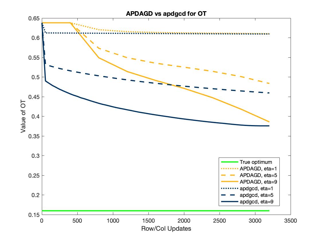
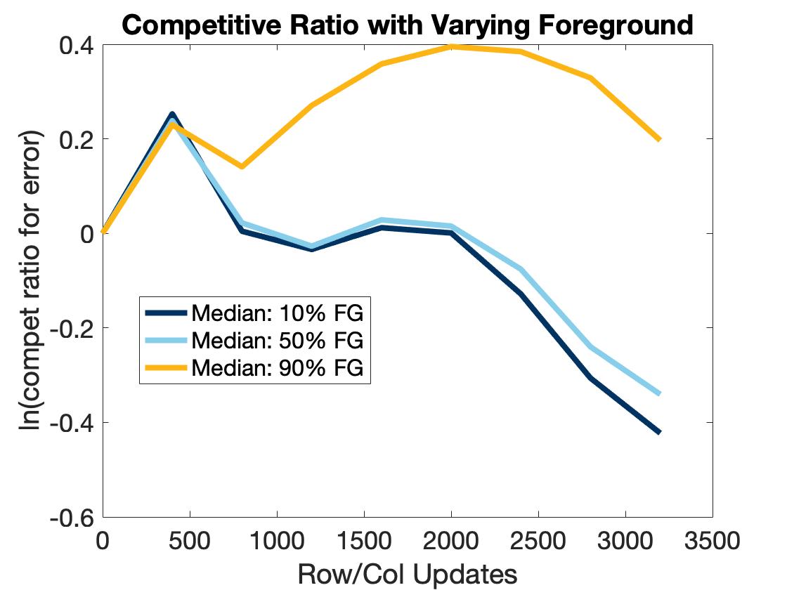
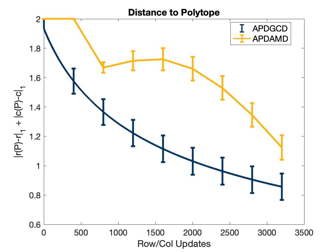
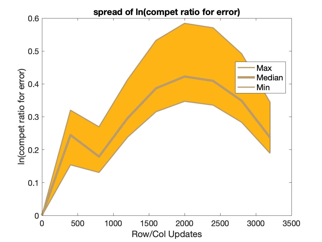
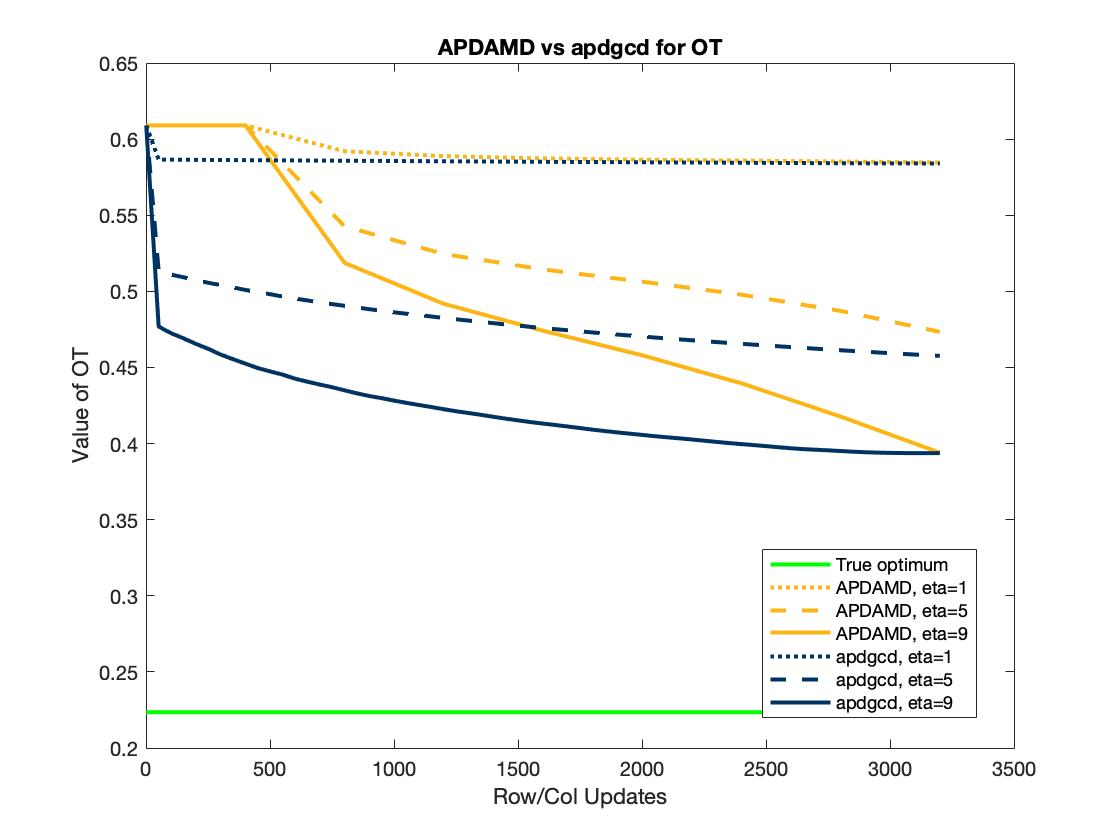
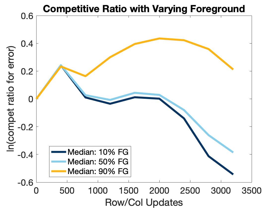
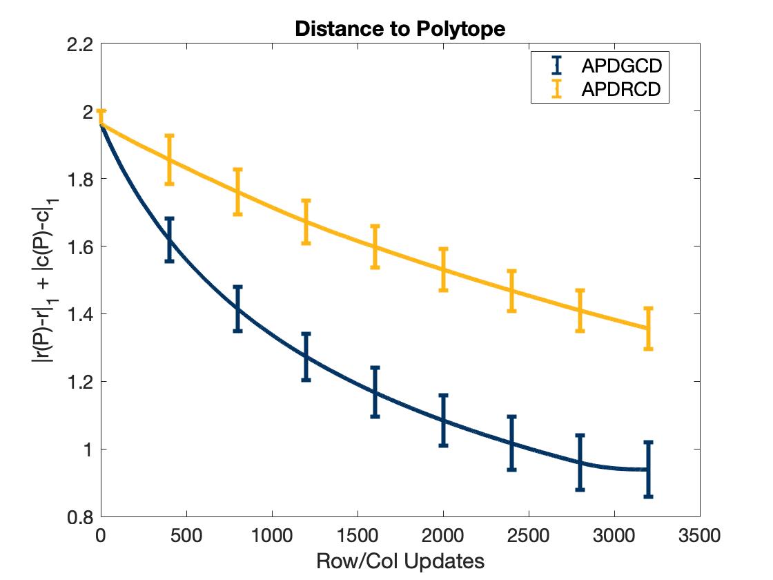
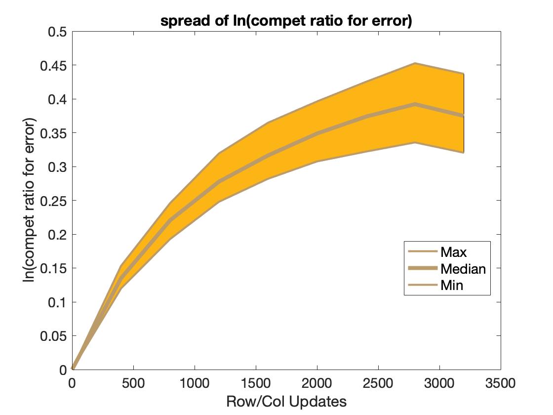
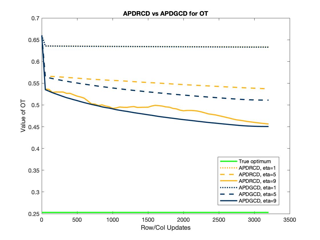
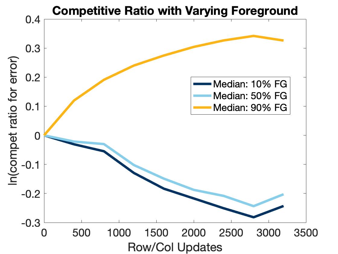
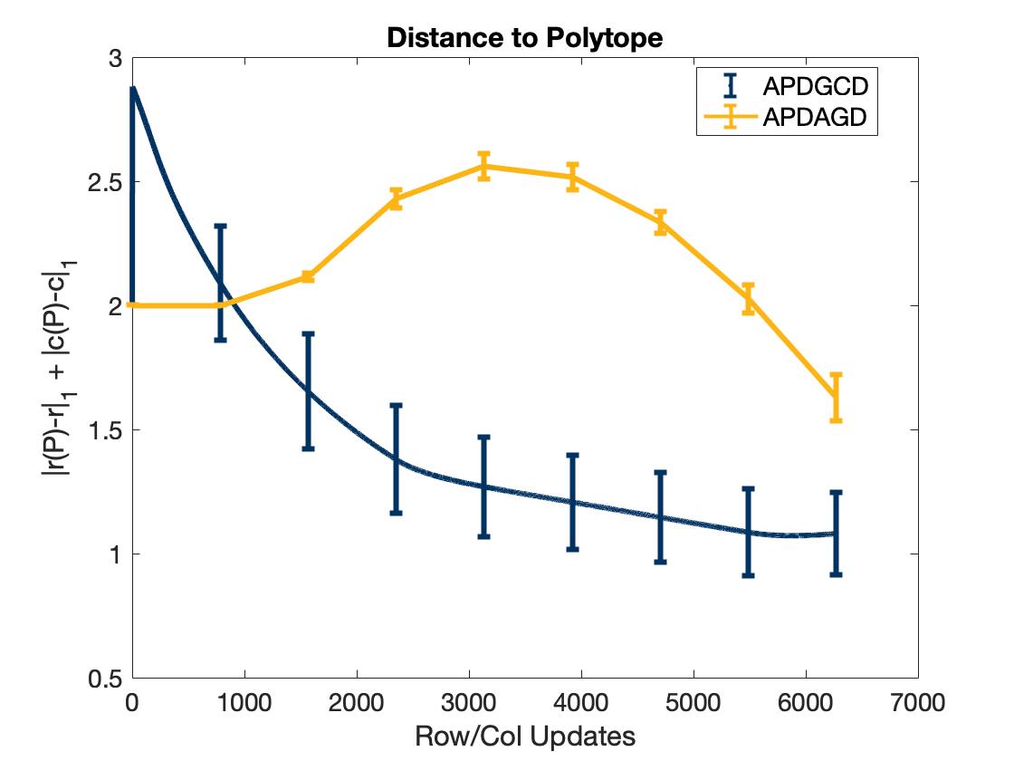
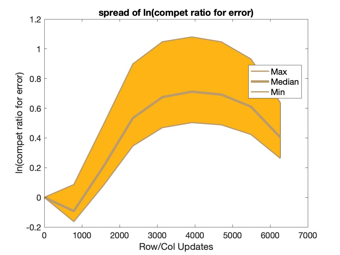
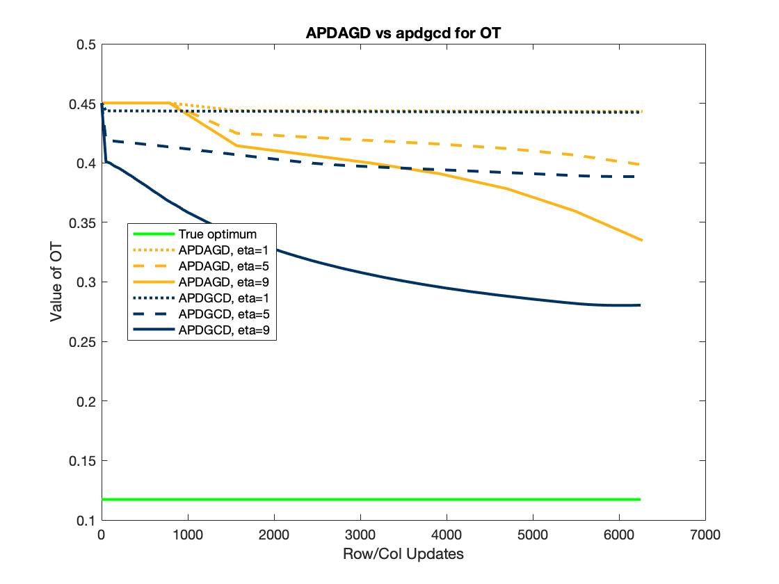
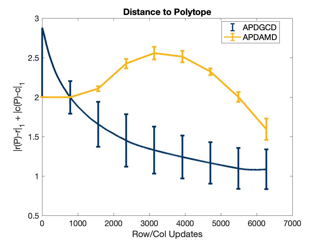
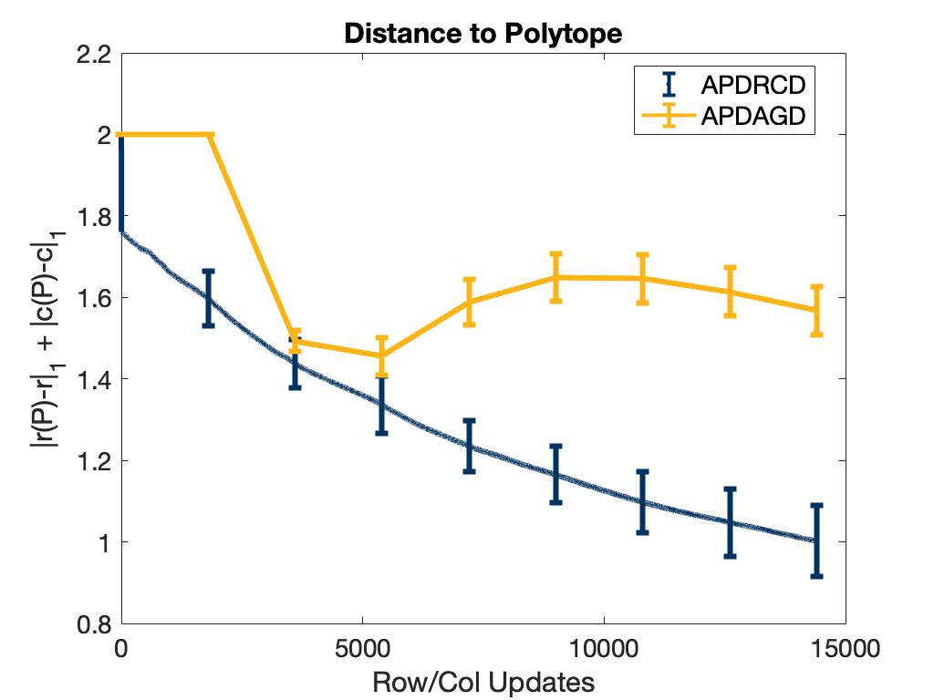
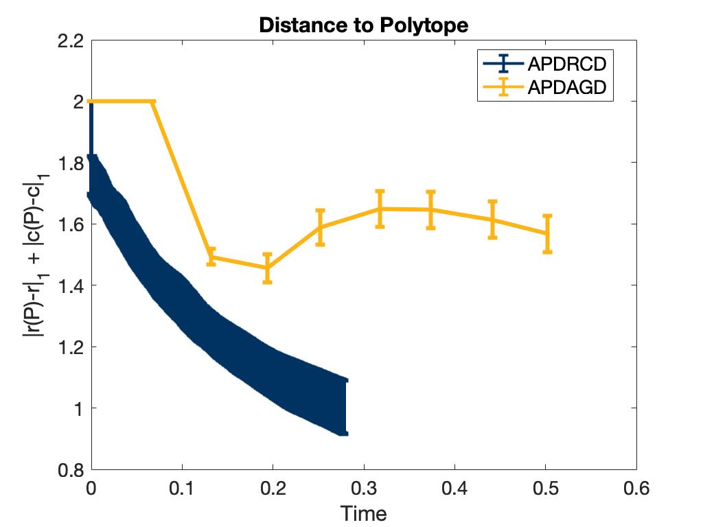
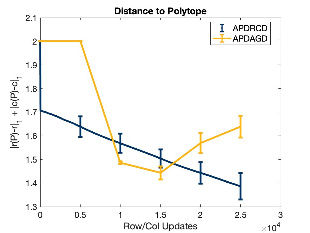
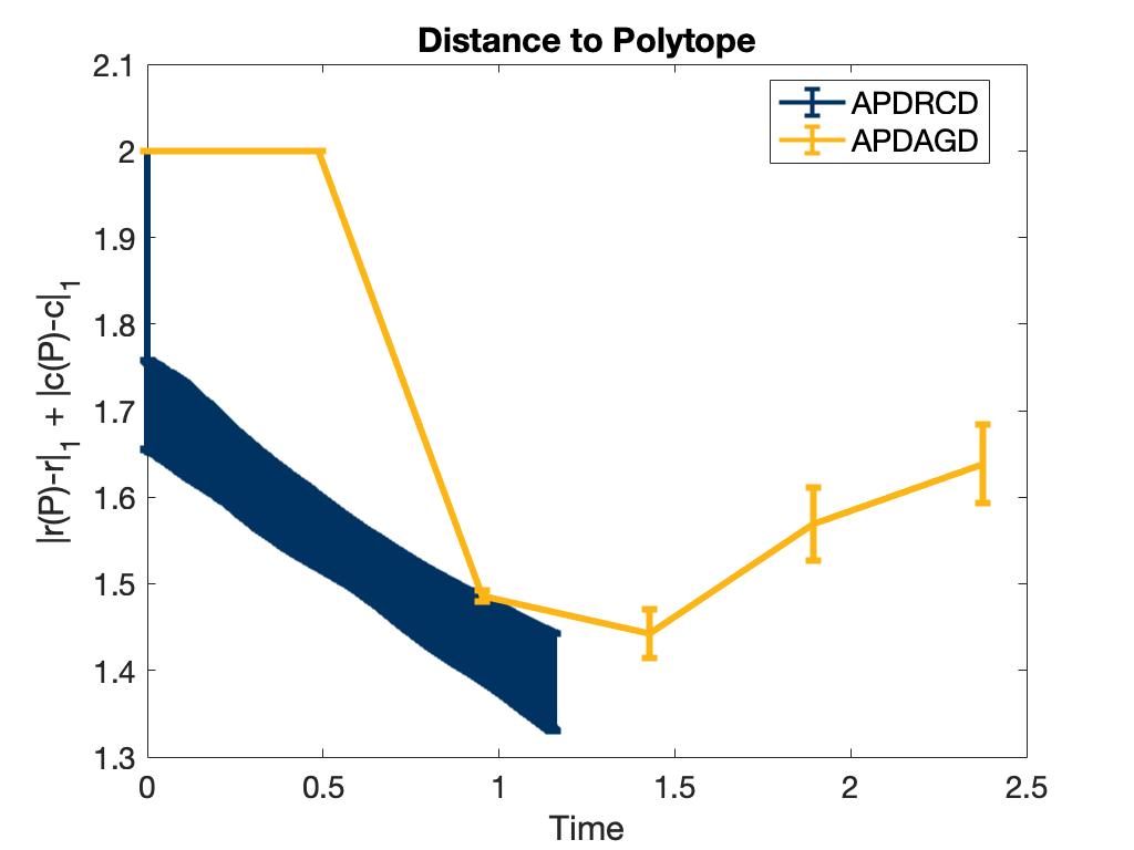
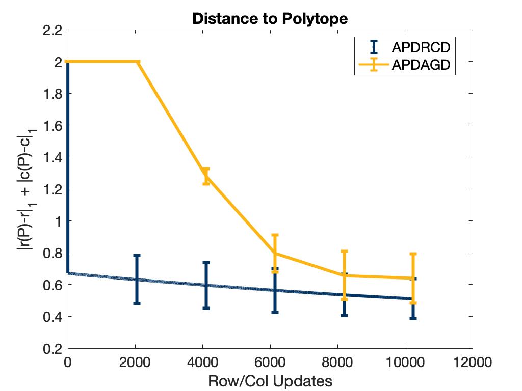
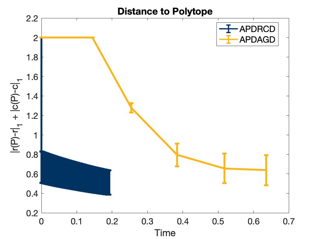
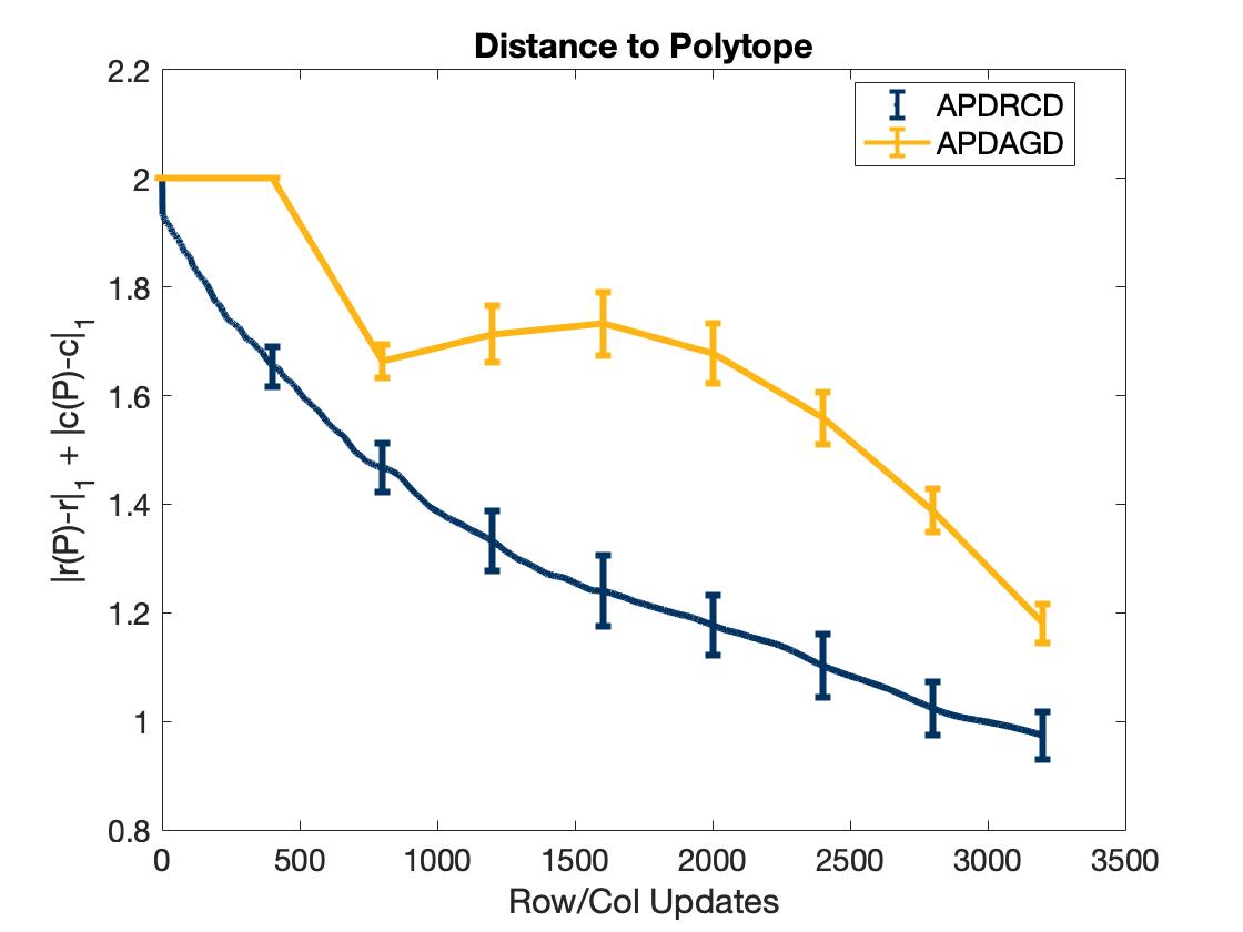
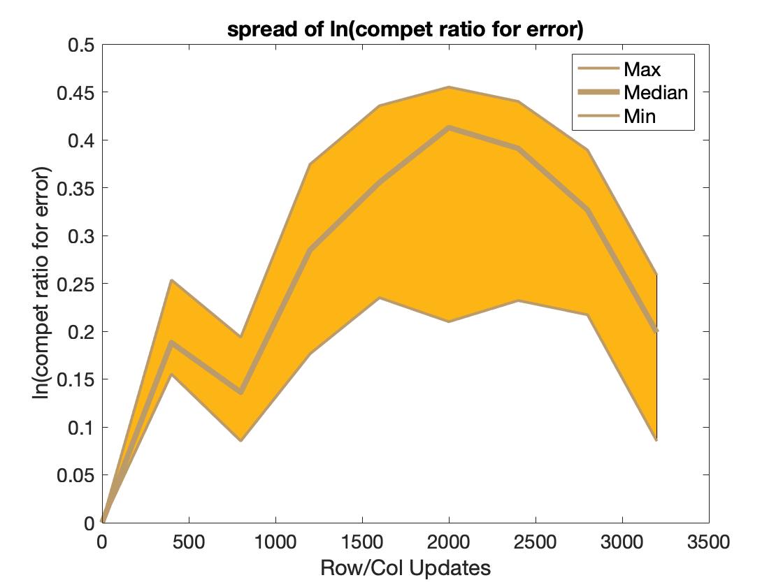
Figure 1: Performance of APDRCD and APDAGD algorithms on the synthetic images. In the top two images, the comparison is based on using the distance $d(P)$ to the transportation polytope, and the maximum, median and minimum of competitive ratios on ten random pairs of images. In the bottom left image, the comparison is based on varying the regularization parameter $\eta\in\{1,5,9\}$ and reporting the optimal value of the original optimal transport problem without entropic regularization. Note that the foreground covers 10% of the synthetic images here. In the bottom right image, we compare the algorithms by using the median of competitive ratios with varying coverage ratio of foreground in the range of $\{0.1,0.5,0.9\}$.

3.3 Accelerated Primal-Dual Greedy Coordinate Descent (APDGCD)

We next present a greedy version of APDRCD algorithm, which we refer to as the accelerated primal-dual greedy coordinate descent (APDGCD) algorithm. The detailed pseudo-code of that algorithm is in Algorithm 3 while an approximating scheme of OT based on the APDGCD algorithm is summarized in Algorithm 4.

Both the APDGCD and APDRCD algorithms follow along the general accelerated primal-dual coordinate descent framework. Similar to the APDRCD algorithm, the algorithmic framework of APDGCD is composed by two main parts: First, instead of performing randomized accelerated coordinate descent on the dual objective function as a subroutine, the APDGCD algorithm chooses the best coordinate that maximizes the absolute value of the gradient of the dual objective function of regularized OT problem among all the coordinates. In the second part, we follow the key averaging step in the APDRCD algorithm by taking a weighted average over the past iterations to get a good approximated solution for the primal problem from the approximated solutions to the dual problem. Since the auxiliary sequence is decreasing, the primal solutions corresponding to the more recent dual solutions have larger weight in this average.

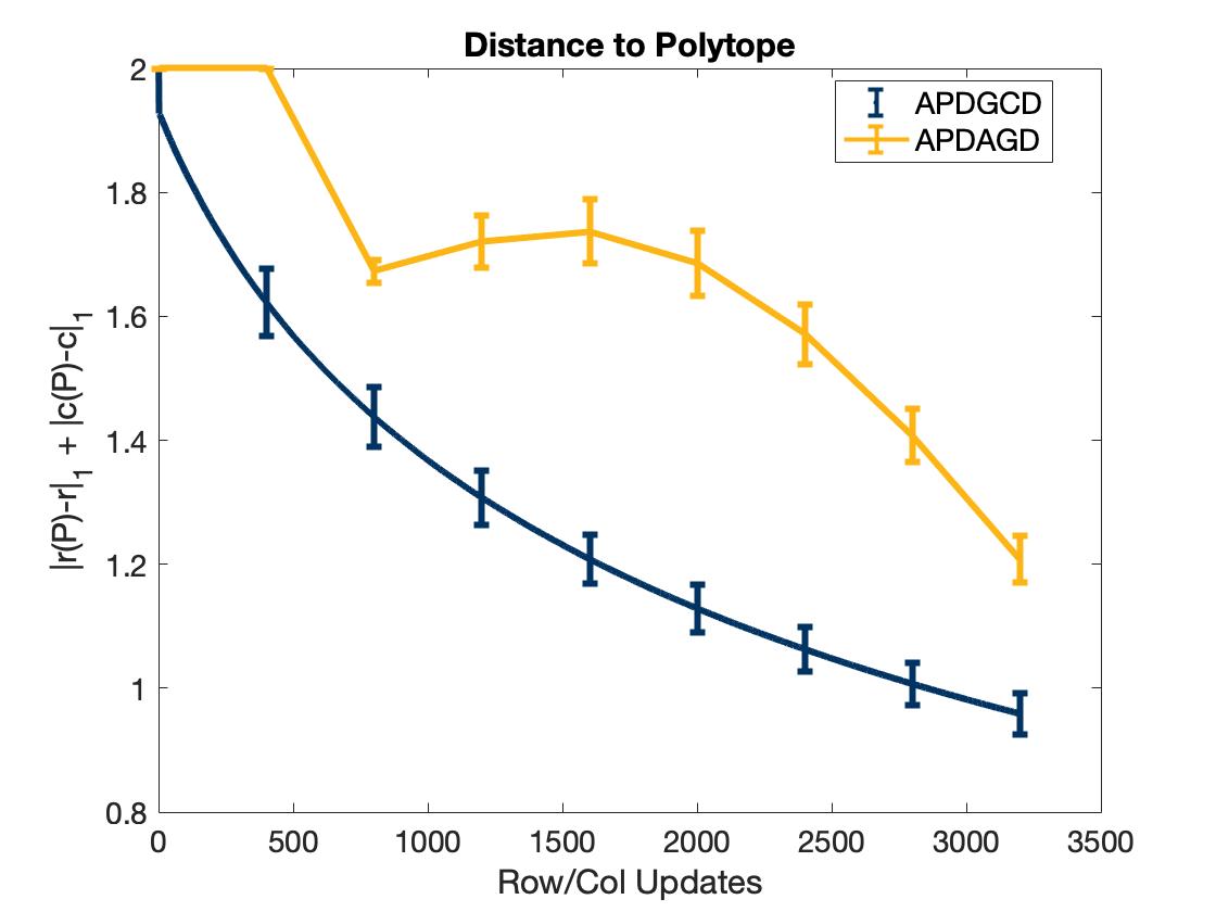
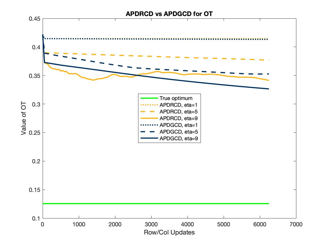
We demonstrate that the APDGCD algorithm enjoys favorable practical performance than APDRCD algorithm on both synthetic and real datasets (cf. Appendix C).

  Input: $\eta=\dfrac{\varepsilon}{4\log(n)}$ and $\varepsilon^{\prime}=\dfrac{\varepsilon}{8\left\|C\right\|_{\infty}}$.

  Step 1: Let $\tilde{r}\in\Delta_{n}$ and $\tilde{l}\in\Delta_{n}$ be defined as

$$\left(\tilde{r},\tilde{l}\right)=\left(1-\frac{\varepsilon^{\prime}}{8}\right)\left(r,l\right)+\frac{\varepsilon^{\prime}}{8n}\left(\textbf{1},\textbf{1}\right).$$

  Step 2: Let $A\in\mathbb{R}^{2n\times n^{2}}$ and $b\in\mathbb{R}^{2n}$ be defined by

$$Avec(X)=\left(\begin{smallmatrix}X\bm{1}\\ X^{T}\bm{1}\end{smallmatrix}\right)\ \ \text{and}\ \ b=\left(\begin{smallmatrix}\tilde{r}\\ \tilde{l}\end{smallmatrix}\right)$$

  Step 3: Compute $\tilde{X}=\text{APDGCD}\left(C,\eta,A,b,\varepsilon^{\prime}/2\right)$ with $\varphi$ defined in 2.2.

  Step 4: Round $\tilde{X}$ to $\hat{X}$ by Algorithm 2 (Altschuler et al., 2017) such that $\hat{X}\textbf{1}=r$, $\hat{X}^{\top}\textbf{1}=l$.

  Output: $\hat{X}$.

Algorithm 4 Approximating OT by APDGCD

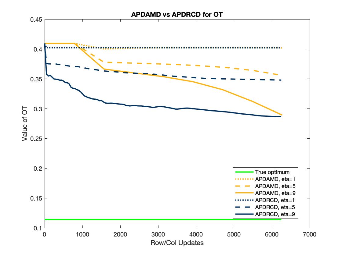
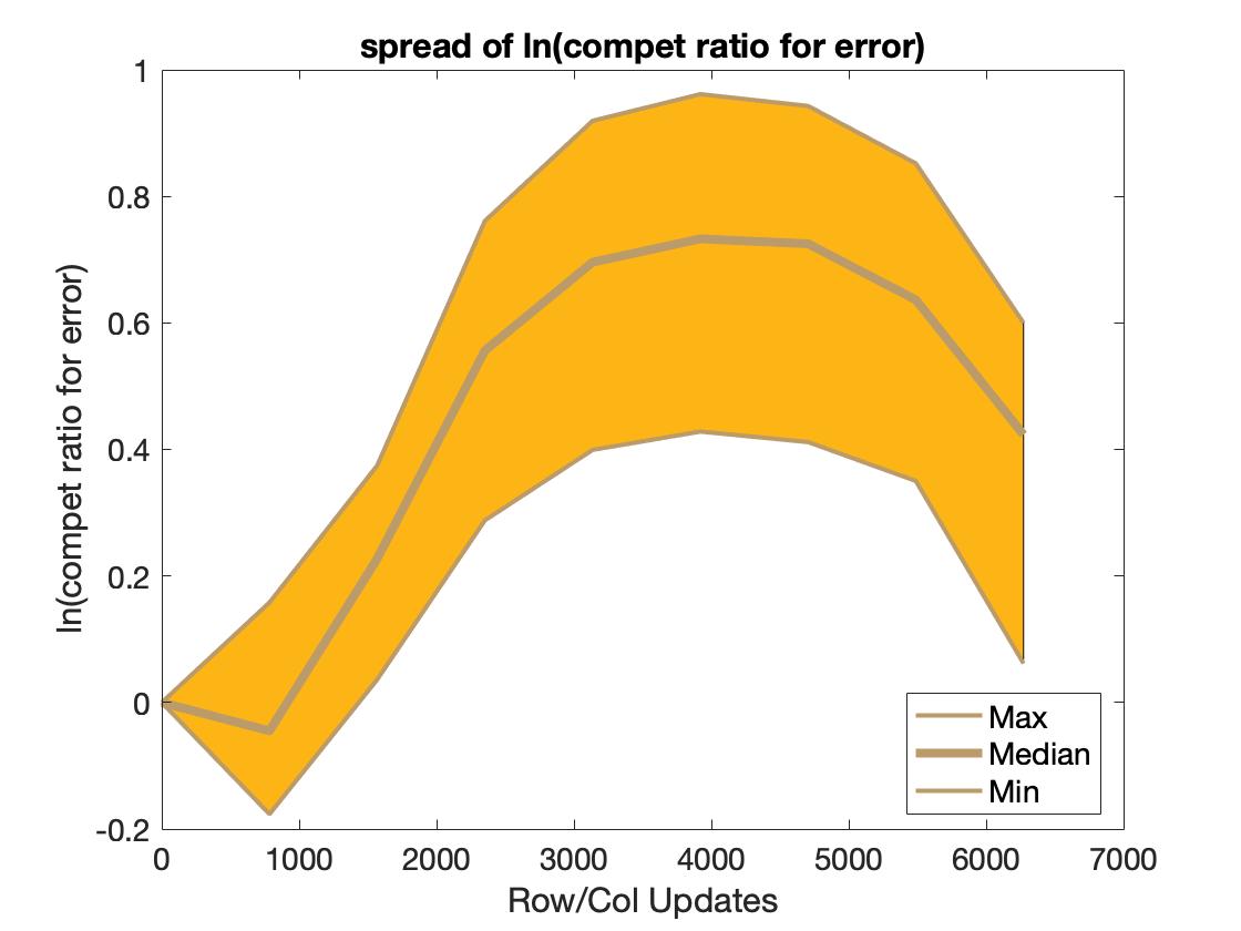
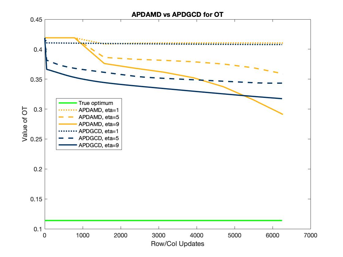
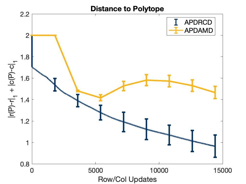
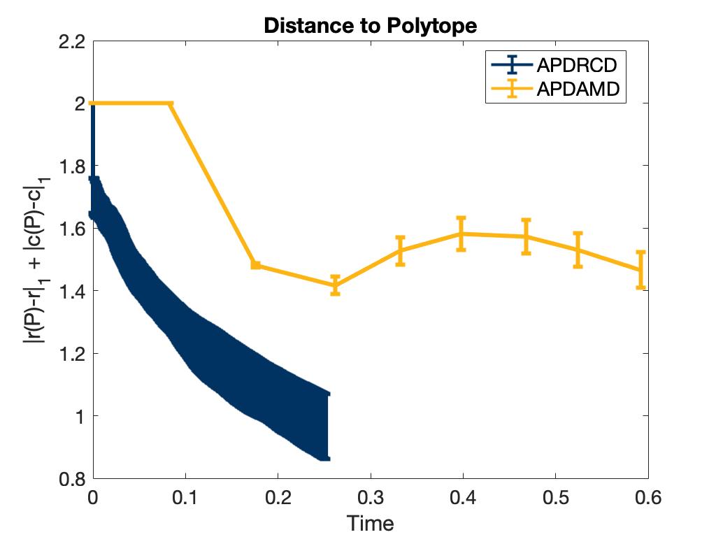
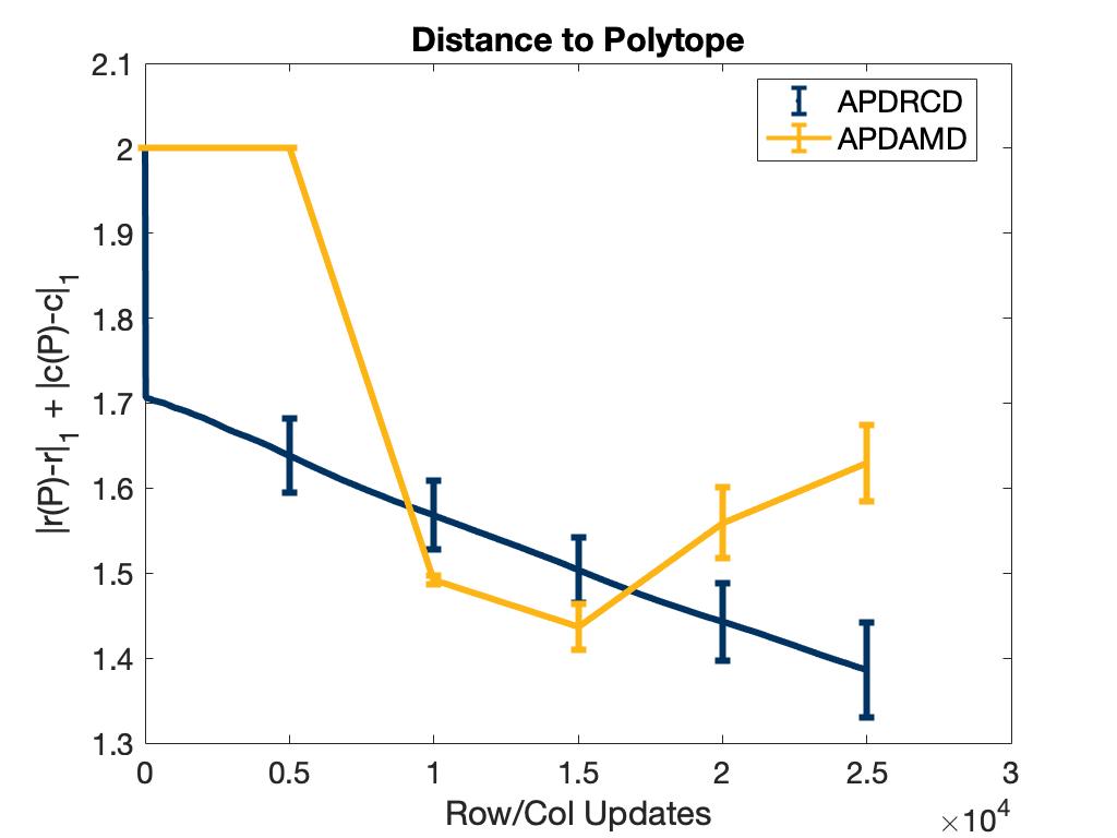
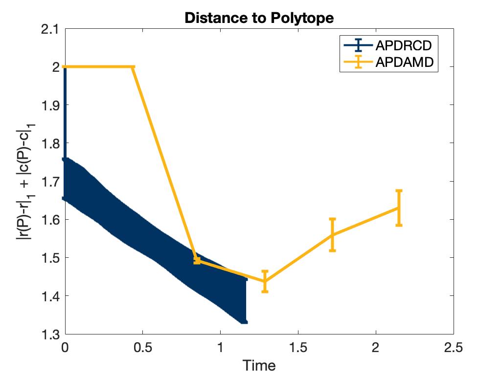
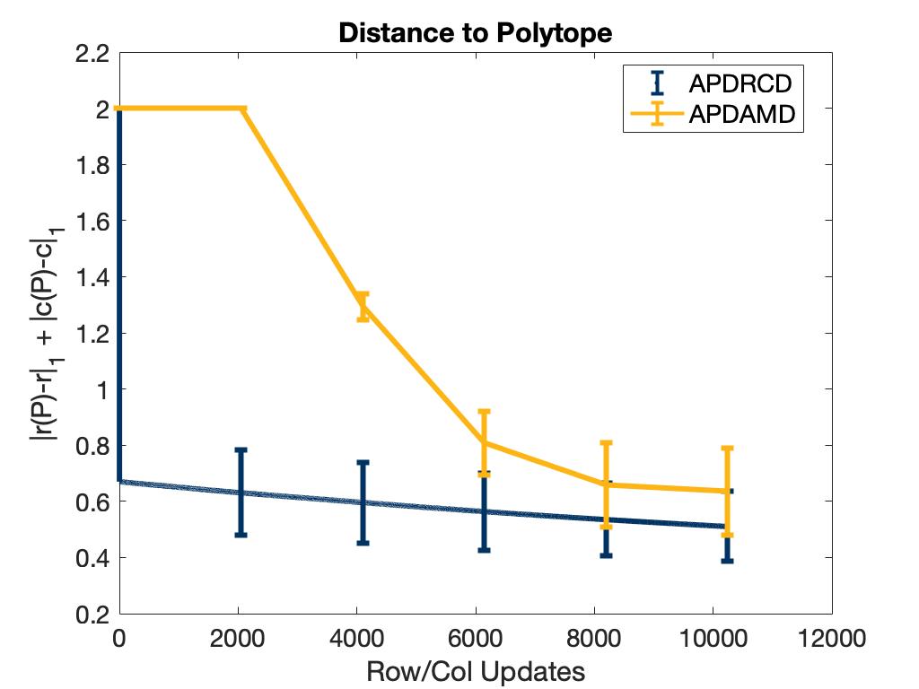
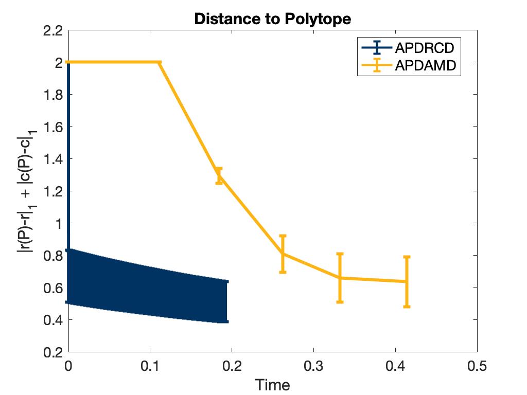
Figure 2: Performance of APDRCD and APDAMD algorithms on the synthetic images. The organization of the images is similar to those in Figure 1.

4 Experiments

We carry out comparative experiments between the APDRCD, APDGCD algorithms and the state-of-art primal-dual algorithms for the OT problem including the APDAGD and APDAMD algorithms, on both synthetic images and the MNIST Digits dataset. Due to space constraints, the comparative experiments between the APDGCD algorithm and APDAGD/APDAMD algorithms, further experiments for the APDRCD algorithm on larger synthetic datasets and CIFAR10 dataset are deferred to Appendix C. Note that for the above comparisons, we also utilize the default linear programming solver in MATLAB to obtain the optimal value of the original optimal transport problem without entropic regularization.

4.1 APDRCD Algorithm with Synthetic Images

We compared the performance of the APDRCD algorithm with the APDAGD and APDAMD algorithms on synthetic images. The generation of synthetic images follows the procedure of (Altschuler et al., 2017; Lin et al., 2019). The images are of size $20\times 20$ and generated by randomly placing a foreground square in the otherwise black background. For the intensities of the background pixels and foreground pixels, we choose uniform distributions on [0,1] and [0, 50] respectively. We vary the proportion of the size of the foreground square in 0.1, 0.5, 0.9 of the full size of the image and implement all the algorithms on different kinds of synthetic images.

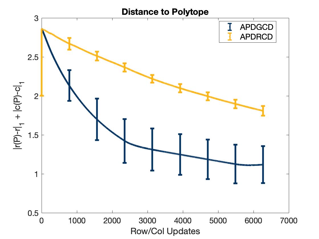
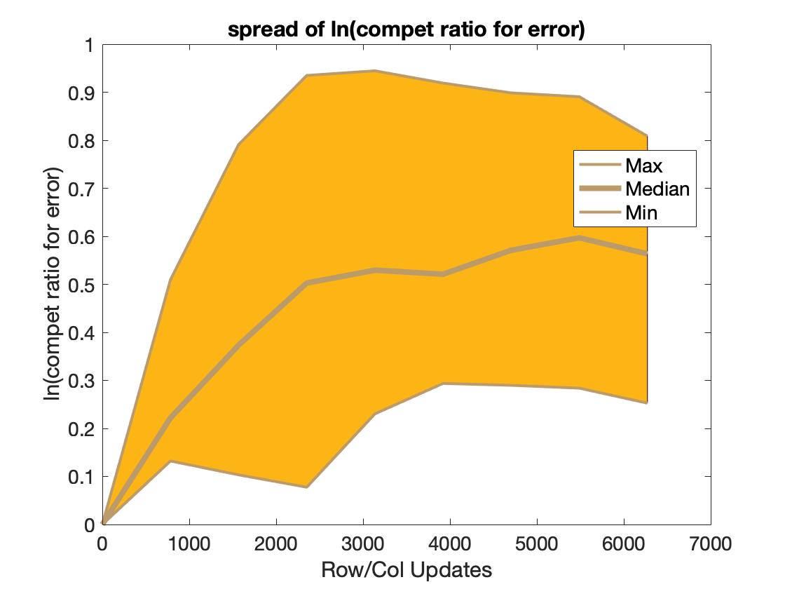
Evaluation metric: We utilize the metrics from (Altschuler et al., 2017). The first metric is the distance between the output of the algorithm and the transportation polytope, $d(X):=||r(X)-r||_{1}+||l(X)-1||_{1}$, where $r(X)$ and $l(X)$ are the row and column marginal vectors of the output matrix $X$ while $r$ and $l$ stand for the true row and column marginal vectors. The second metric is the competitive ratio, defined by $\log(\frac{d(X1)}{d(X2)})$ where $d(X1)$ and $d(X2)$ refer to the distance between the outputs of two algorithms and the transportation polytope.

Figure 3: Performance of the APDRCD, APDAGD and APDAMD algorithms on the MNIST images. In the first row of images, we compare the APDRCD and APDAGD algorithms in terms of iteration counts. The leftmost image specifies the distances $d(P)$ to the transportation polytope for two algorithms; the middle image specifies the maximum, median and minimum of competitive ratios on ten random pairs of MNIST images; the rightmost image specifies the values of regularized OT with varying regularization parameter $\eta=\{1,5,9\}$. In addition, the second row of images present comparative results for APDRCD versus APDAMD.

Experimental settings and results: We perform two pairwise comparative experiments for the APDRCD algorithm versus the APDAGD and APDAMD algorithms by running these algorithms with ten randomly selected pairs of synthetic images. We also evaluate all the algorithms with varying regularization parameter $\eta\in\{1,5,9\}$ and the optimal value of the original OT problem without the entropic regularization, as suggested by (Altschuler et al., 2017; Lin et al., 2019).

We present the results in Figure 1 and Figure 2. The APDRCD algorithm has better performance than the APDAGD and APDAMD algorithms in terms of the iterations. When the number of iterations is small, the APDRCD algorithm achieves faster and more stable decrements than the other two algorithms with regard to both the distance to polytope and the value of OT during the computing process, which is beneficial for the purposes of tuning and illustrates the advantage of using randomized coordinate descent on the dual regularized problem.

4.2 APDRCD Algorithm with MNIST Images

We compare the APDRCD algorithm and the APDAGD and APDAMD algorithms on MNIST images with the same set of evaluation metrics. The image pre-processing follows the same pre-processing procedure as suggested in (Lin et al., 2019). We omit the details for the sake of brevity.

We present the results with the MNIST images in Figure 3 with various values for the regularization parameter $\eta\in\{1,5,9\}$. We also evaluate the algorithms with the optimal value of the original OT problem without entropic regularization. As shown in Figure 3, the APDRCD algorithm outperforms both the APDAGD and APDAMD algorithms on the MNIST dataset in terms of the number of iterations. Additionally, the APDRCD algorithm displays faster and smoother convergence than the other algorithms at small iteration numbers with regard to both the evaluation metrics, which implies the advantage that it is easier to be tuned in practice.

5 Discussion

We have proposed and analyzed new accelerated primal-dual coordinate descent algorithms for approximating the optimal transport distance between two discrete probability measures. These accelerated primal-dual coordinate descent algorithms have comparable theoretical complexity as that of existing accelerated primal-dual algorithms while enjoying better experimental performance. Furthermore, we show that the APDRCD and APDGCD algorithms are suitable for other large-scale problems apart from computing the OT distance; we propose extensions that approximate the Wasserstein barycenters for multiple probability distributions.

There are several directions for future work. Given the favorable practical performance of the APDRCD and the APDGCD algorithms over existing primal-dual algorithms, it is of interest to carry out more experiments of the distributed APDRCD and APDGCD algorithms for computing Wasserstein barycenters. Another important direction is to construct fast distributed algorithms for the case of time-varying and directed machine networks to approximate the Wasserstein barycenters. It remains as an interesting and important open research question how the dynamics of the network affect the performance of these algorithms.

Acknowledgements

We thank Tianyi Lin for many helpful discussions. This work was supported in part by the Mathematical Data Science program of the Office of Naval Research under grant number N00014-18-1-2764.

Appendix

In the appendix, we first provide detailed proofs of all the remaining results in Section A. Then, we present an application of APDRCD and APDGCD algorithms for the Wasserstein barycenter problem in Section B. Finally, further comparative experiments between APDGCD algorithm versus APDRCD, APDAGD and APDAMD algorithms, and experiments on larger synthetic image datasets and CIFAR10 dataset are in Section C.

Appendix A Proofs for all results

In this appendix, we provide the complete proofs for remaining results in the main text.

A.1 Proof of Lemma 3.2

By Eq. (5), we have the following equations

$$|\nabla\varphi_{i_{k}}(y^{k})|^{2}$$

$$=2|\nabla\varphi_{i_{k}}(y^{k})|^{2}-|\nabla\varphi_{i_{k}}(y^{k})|^{2}$$

$$=2L\big{(}y_{i_{k}}^{k}-\lambda_{i_{k}}^{k+1}\big{)}\nabla_{i_{k}}\varphi(y^{k})-L^{2}(\lambda_{i_{k}}^{k+1}-y_{i_{k}}^{k+1})^{2}.$$

Combining the above equations with Lemma 3.1, we have

$$\varphi(\lambda^{k+1})$$

$$\leq\varphi(y^{k})-\frac{1}{2L}(\nabla_{i_{k}}\varphi(y^{k}))^{2}$$

$$=\varphi(y^{k})+(\lambda_{i_{k}}^{k+1}-y_{i_{k}}^{k})\nabla_{i_{k}}\varphi(y^{k})+\frac{L}{2}(\lambda_{i_{k}}^{k+1}-y_{i_{k}}^{k+1})^{2}.$$ (9)

Furthermore, the results from Eq. (5) and Eq. (6) lead to the following equations

$$\lambda_{i_{k}}^{k+1}-y_{i_{k}}^{k} =-\frac{1}{L}\nabla_{i_{k}}\varphi(y^{k}),$$

$$z_{i_{k}}^{k+1}-z_{i_{k}}^{k} =-\frac{1}{2nL\theta_{k}}\nabla_{i_{k}}\varphi(y^{k}).$$

Therefore, we have

$$\lambda_{i_{k}}^{k+1}-y_{i_{k}}^{k}=2n\theta_{k}(z_{i_{k}}^{k+1}-z_{i_{k}}^{k}).$$

The above equation together with Eq. (A.1) yields the following inequality

$$\varphi(\lambda^{k+1})$$

$$\leq\varphi(y^{k})+2n\theta_{k}\big{(}z_{i_{k}}^{k+1}-z_{i_{k}}^{k}\big{)}\nabla_{i_{k}}\varphi_{i_{k}}(y^{k})$$

$$+2n^{2}L\theta_{k}^{2}\big{(}z_{i_{k}}^{k+1}-z_{i_{k}}^{k}\big{)}^{2}.$$ (10)

By the result of Eq. (6), we have

$$(z_{i_{k}}^{k+1}-z_{i_{k}}^{k})+\frac{1}{2nL\theta_{k}}\nabla_{i_{k}}\varphi(y^{k})=0.$$

Therefore, for any $\lambda\in\mathbb{R}^{2n}$, we find that

$$(\lambda_{i_{k}}-z_{i_{k}}^{k+1})[(z_{i_{k}}^{k+1}-z_{i_{k}}^{k})+\frac{1}{2nL\theta_{k}}\nabla_{i_{k}}\varphi(y^{k})]=0.$$

Note that the above equation is equivalent to the following:

$$\frac{1}{nL\theta_{k}}(\lambda_{i_{k}}-z_{i_{k}}^{k+1})\nabla_{i_{k}}\varphi(y^{k})$$

$$=-2(\lambda_{i_{k}}-z_{i_{k}}^{k+1})(z_{i_{k}}^{k+1}-z_{i_{k}}^{k})$$

$$=(\lambda_{i_{k}}-z_{i_{k}}^{k+1})^{2}-(\lambda_{i_{k}}-z_{i_{k}}^{k})^{2}+(z_{i_{k}}^{k+1}-z_{i_{k}}^{k})^{2}$$

where the second equality in the above display comes from simple algebra. Rewriting the above equality, we have:

$$(z_{i_{k}}^{k+1}-z_{i_{k}}^{k})^{2}$$

$$=\frac{1}{nL\theta_{k}}(\lambda_{i_{k}}-z_{i_{k}}^{k+1})\nabla_{i_{k}}\varphi(y^{k})$$

$$-(\lambda_{i_{k}}-z_{i_{k}}^{k+1})^{2}+(\lambda_{i_{k}}-z_{i_{k}}^{k})^{2}$$

Combining the above equation with Eq. (A.1) yields the following inequality:

$$\varphi(\lambda^{k+1})$$

$$\leq\varphi(y^{k})+2n\theta_{k}(\lambda_{i_{k}}-z_{i_{k}}^{k})\nabla_{i_{k}}\varphi(y^{k})$$

$$+2n^{2}L\theta^{2}_{k}\biggr{[}(\lambda_{i_{k}}-z_{i_{k}}^{k})^{2}-(\lambda_{i_{k}}-z_{i_{k}}^{k+1})^{2}\biggr{]}.$$ (11)

Recall the definition of $y^{k}$ in Step 3 of Algorithm 1 as follows:

$$y^{k}=(1-\theta_{k})\lambda^{k}+\theta^{k}z^{k},$$

which can be rewritten as:

$$\theta_{k}(\lambda-z^{k})=\theta_{k}(\lambda-y^{k})+(1-\theta_{k})(\lambda^{k}-y^{k})$$ (12)

for any $\lambda\in\mathbb{R}^{2n}$.

The above equation implies that

$$\varphi(y^{k})+\theta_{k}(\lambda-z^{k})^{T}\nabla\varphi(y^{k})$$

$$\leq\theta_{k}[\varphi(y^{k})+(\lambda-y^{k})^{T}\nabla\varphi(y^{k})]$$

$$+(1-\theta_{k})[\varphi(y^{k})+(\lambda^{k}-y^{k})^{T}\nabla\varphi(y^{k})]$$

$$\leq\theta_{k}[\varphi(y^{k})+(\lambda-y^{k})^{T}\nabla\varphi(y^{k})]+(1-\theta_{k})\varphi(\lambda^{k})$$

where the last inequality comes from the convexity of $\varphi$. Combining this equation and taking expectation over $i_{k}$ for the first two terms of Eq. (A.1), we have:

$$\varphi(y^{k})+(2n\theta_{k})\mathbb{E}_{i_{k}}[(\lambda_{i_{k}}-z_{i_{k}}^{k})\nabla_{i_{k}}\varphi(y^{k})]$$

$$=\varphi(y^{k})+\theta_{k}(\lambda-z^{k})^{T}\nabla\varphi(y^{k})$$

$$\leq\theta_{k}[\varphi(y^{k})+(\lambda-y^{k})^{T}\nabla\varphi(y^{k})]+(1-\theta_{k})\varphi(\lambda^{k})$$ (13)

where we use Eq. (12) and the convexity of the dual function in the last step. For the last term in the right hand side of Eq. (A.1), by taking expectation over $i_{k}$, we have:

$$\mathbb{E}_{i_{k}}\biggr{[}2n^{2}L\theta^{2}_{k}\bigr{[}(\lambda_{i_{k}}-z_{i_{k}}^{k})^{2}-(\lambda_{i_{k}}-z_{i_{k}}^{k+1})^{2}\bigr{]}\biggr{]}$$

$$=2n^{2}L\theta_{k}^{2}\mathbb{E}_{i_{k}}\bigr{[}||\lambda-z^{k}||^{2}-||\lambda-z^{k+1}||^{2}\bigr{]}$$ (14)

where the last equality comes from the following equations:

$$\mathbb{E}_{i_{k}}\bigr{[}(\lambda_{i_{k}}-z_{i_{k}}^{k})^{2}-\bigr{(}\lambda_{i_{k}}-z_{i_{k}}^{k+1}\bigr{)}^{2}\bigr{]}$$

$$=\mathbb{E}_{i_{k}}\biggr{[}(\lambda_{i_{k}}-z_{i_{k}}^{k})^{2}-\biggr{(}\lambda_{i_{k}}-z_{i_{k}}^{k}+\frac{1}{2nL\theta_{k}}\nabla_{i_{k}}\varphi(y^{k})\biggr{)}^{2}\biggr{]}$$

$$=\frac{1}{2n}(\|\lambda-z^{k}\|^{2}-\sum_{i_{k}=0}^{2n}\biggr{(}\lambda_{i_{k}}-z_{i_{k}}^{k}+\frac{1}{2nL\theta_{k}}\nabla_{i_{k}}\varphi(y^{k})\biggr{)}^{2})$$

$$=\frac{1}{2n}\|\lambda-z^{k}\|^{2}-\frac{1}{2n}\|\lambda-z^{k}+\frac{1}{2nL\theta_{k}}\nabla\varphi(y^{k})\|^{2}$$

$$=\frac{1}{2n}\biggr{[}-\frac{(\lambda-z^{k})}{nL\theta_{k}}\nabla\varphi(y^{k})-\frac{1}{4n^{2}L^{2}\theta_{k}^{2}}\|\nabla\varphi(y^{k})\|^{2}\biggr{]}$$

$$=(-2)(\lambda-z^{k})\mathbb{E}_{i_{k}}[z^{k}-z^{k+1}]-\mathbb{E}_{i_{k}}[||z^{k}-z^{k+1}||^{2}]$$

where the last inequality is due to the fact that $\nabla\varphi(y^{k})=4\mathbb{E}_{i_{k}}[(z^{k}-z^{k+1})n^{2}L\theta_{k}]$ and Jensen’s inequality. Therefore, by simple algebra, we have

$$\mathbb{E}_{i_{k}}\biggr{[}(\lambda_{i_{k}}-z_{i_{k}}^{k})^{2}-(\lambda_{i_{k}}-z_{i_{k}}^{k+1})^{2}\biggr{]}$$

$$=(-2)(\lambda-z^{k})\mathbb{E}_{i_{k}}[z^{k}-z^{k+1}]-\mathbb{E}_{i_{k}}[||z^{k}-z^{k+1}||^{2}]$$

$$=\mathbb{E}_{i_{k}}[\|\lambda-z^{k}\|^{2}-\|\lambda-z^{k+1}\|^{2}].$$

Notice that equation (A.1) holds for any value of $i_{k}$. Hence, by combining the results from Eq. (A.1) and Eq. (A.1) with Eq. (A.1), at each iteration with a certain value of $i_{k}$, we obtain that

$$\mathbb{E}_{i_{k}}[\varphi(\lambda^{k+1})]$$

$$\leq(1-\theta_{k})\varphi(\lambda^{k})+\theta_{k}[\varphi(y^{k})+(\lambda-y^{k})^{\top}\nabla\varphi(y^{k})]$$

$$+2n^{2}L\theta_{k}^{2}\biggr{(}||\lambda-z^{k}||^{2}-\mathbb{E}_{i_{k}}[||\lambda-z^{k+1}||^{2}]\biggr{)}.$$

As a consequence, we achieve the conclusion of the lemma.

Figure 4: Performance of APDGCD and APDAGD algorithms on the synthetic images. The organization of the images is similar to those in Figure 1.

A.2 Proof of Theorem 3.3

By the result of Lemma 3.2 and the definition of the sequence $\{\theta_{k}\}$ in Algorithm 1, we obtain the following bounds:

$$\mathbb{E}\biggr{[}\frac{1}{\theta_{k}^{2}}\varphi(\lambda^{k+1})\biggr{]}$$

$$\leq\mathbb{E}\biggr{[}\frac{1-\theta_{k}}{=}{\theta_{k}^{2}}\varphi(\lambda^{k})+\frac{1}{\theta_{k}}[\varphi(y^{k})+(\lambda-y^{k})^{T}\nabla\varphi(y^{k})]$$

$$+2Ln^{2}\big{(}||\lambda-z^{k}||^{2}-||\lambda-z^{k+1}||^{2}\big{)}\biggr{]}$$

$$=\mathbb{E}\biggr{[}\frac{1}{\theta_{k-1}^{2}}\varphi(\lambda^{k})+\frac{1}{\theta_{k}}[\varphi(y^{k})+(\lambda-y^{k})^{T}\nabla\varphi(y^{k})]$$

$$+2Ln^{2}\big{(}||\lambda-z^{k}||^{2}-||\lambda-z^{k+1}||^{2}\big{)}\biggr{]}$$

where the outer expectations are taken with respect to the random sequence of the coordinate indices in Algorithm 1. Keep iterating the above bound and using the fact that $\theta_{0}=1$ and $C_{k}=1/\theta_{k}^{2}$, we arrive at the following inequalities:

$$C_{k}\mathbb{E}\big{[}\varphi(\lambda^{k+1})\big{]}$$

$$\leq\sum_{i=0}^{k}\dfrac{1}{\theta_{i}}\mathbb{E}\big{[}\varphi(y^{i})+\left\langle\nabla\varphi(y^{i}),\lambda-y^{i}\right\rangle\big{]}$$

$$+2Ln^{2}\bigr{(}||\lambda-z^{0}||^{2}-\mathbb{E}\big{[}||\lambda-z^{k+1}||^{2}\big{]}\bigr{)}$$

$$\leq\min\limits_{\lambda\in\mathbb{R}^{2n}}\biggr{(}\sum_{i=0}^{k}\dfrac{1}{\theta_{i}}\mathbb{E}\big{[}\varphi(y^{i})+\left\langle\nabla\varphi(y^{i}),\lambda-y^{i}\right\rangle\big{]}$$

$$+2Ln^{2}\bigr{(}||\lambda-z^{0}||^{2}-\mathbb{E}\big{[}||\lambda-z^{k+1}||^{2}\big{]}\bigr{)}\biggr{)}$$

$$\leq\min\limits_{\lambda\in B_{2}(2\hat{R})}\biggr{(}\sum_{i=0}^{k}\dfrac{1}{\theta_{i}}\mathbb{E}\big{[}\varphi(y^{i})+\left\langle\nabla\varphi(y^{i}),\lambda-y^{i}\right\rangle\big{]}$$

$$+2Ln^{2}\bigr{(}||\lambda-z^{0}||^{2}-\mathbb{E}\big{[}||\lambda-z^{k+1}||^{2}\big{]}\bigr{)}\biggr{)}$$

where $\hat{R}:=\eta\sqrt{n}(R+\frac{1}{2})$ is the upper bound for $l_{2}$-norm of optimal solutions of dual regularized OT problem (2.2) according to Lemma 3.2 in (Lin et al., 2019) and $\mathbb{B}_{2}(r)$ is defined as

$$\mathbb{B}_{2}(r):=\{\lambda\in\mathbb{R}^{2n}\ |\ ||\lambda||_{2}\leq r\}.$$

As $\mathbb{E}\big{[}||\lambda-z^{k+1}||^{2}\big{]}\geq 0$, the inequality in the above display can be further rewritten as

$$C_{k}\mathbb{E}\big{[}\varphi(\lambda^{k+1})\big{]}$$

$$\leq\min\limits_{\lambda\in\mathbb{B}_{2}(2\hat{R})}\biggr{(}\sum_{i=0}^{k}\dfrac{1}{\theta_{i}}\mathbb{E}\big{[}\varphi(y^{i})+\left\langle\nabla\varphi(y^{i}),\lambda-y^{i}\right\rangle\big{]}$$

$$+2Ln^{2}||\lambda-z^{0}||^{2}\biggr{)}$$

$$\leq\min\limits_{\lambda\in\mathbb{B}_{2}(2\hat{R})}\biggr{(}\sum_{i=0}^{k}\dfrac{1}{\theta_{i}}\mathbb{E}\big{[}\varphi(y^{i})+\left\langle\nabla\varphi(y^{i}),\lambda-y^{i}\right\rangle\big{]}$$

$$+8Ln^{2}\hat{R}^{2}\biggr{)}$$ (15)

where the last inequality is due to $z^{0}=0$. Furthermore, by the definition of the dual entropic regularized OT objective function $\varphi(\lambda)$, we can verify the following equations:

$$\varphi(y^{i})+\left\langle\nabla\varphi(y^{i}),\lambda-y^{i}\right\rangle$$

$$=\left\langle y^{i},b-Ax(y^{i})\right\rangle-f(x(y^{i}))+\left\langle\lambda-y^{i},b-Ax(y^{i})\right\rangle$$

$$=-f(x(y^{i}))+\left\langle\lambda,b-Ax(y^{i})\right\rangle$$

where $f(x):=\left\langle C,x\right\rangle$, $x(\lambda):=\mathop{\arg\max}\limits_{x\in\mathbb{R}^{n\times n}}\biggr{\{}-f(x)-\left\langle A^{\top}\lambda,x\right\rangle\biggr{\}}$, and $b=\begin{pmatrix}r\\ l\end{pmatrix}$. The above equation leads to the following inequality:

$$\sum_{i=0}^{k}\dfrac{1}{\theta_{i}}\mathbb{E}\big{[}\varphi(y^{i})+\left\langle\nabla\varphi(y^{i}),\lambda-y^{i}\right\rangle\big{]}$$

$$=\sum_{i=0}^{k}\dfrac{1}{\theta_{i}}\mathbb{E}\big{[}-f(x(y^{i}))+\left\langle\lambda,b-Ax(y^{i})\right\rangle\big{]}$$

$$\leq-C_{k}f(\mathbb{E}\big{[}x^{k}\big{]})+\sum_{i=0}^{k}\dfrac{1}{\theta_{i}}\left\langle\lambda,b-A\mathbb{E}\big{[}x(y^{i})\big{]}\right\rangle$$

$$=\ C_{k}\big{(}-f(\mathbb{E}\big{[}x^{k}\big{]})+\left\langle\lambda,b-A\mathbb{E}\big{[}x^{k}\big{]}\right\rangle\big{)}$$ (16)

where the second inequality is due to the convexity of $f$. Combining the results from (15) and (16), we achieve the following bound

$$C_{k}\mathbb{E}\big{[}\varphi(\lambda^{k+1})\big{]}$$

$$\leq-C_{k}f(\mathbb{E}\big{[}x^{k}\big{]})+\min\limits_{\lambda\in\mathbb{B}_{2}(2\hat{R})}\{C_{k}\left\langle\lambda,b-A\mathbb{E}\big{[}x^{k}\big{]}\right\rangle\}$$

$$+8Ln^{2}\hat{R}^{2}$$

$$\leq-C_{k}f(\mathbb{E}\big{[}x^{k}\big{]})+8Ln^{2}\hat{R}^{2}-2C_{k}\hat{R}\mathbb{E}\big{[}||Ax^{k}-b||_{2}\big{]}.$$

which is equivalent to

$$f(\mathbb{E}\big{[}x^{k}\big{]})+\mathbb{E}\big{[}\varphi(\lambda^{k+1})\big{]}+2\hat{R}\mathbb{E}\big{[}||Ax^{k}-b||_{2}\big{]}$$

$$\leq\frac{8Ln^{2}\hat{R}^{2}}{C_{k}}.$$ (17)

Figure 5: Performance of APDGCD and APDAMD algorithms on the synthetic images. The organization of the images is similar to those in Figure 5.

Denoting $\lambda^{*}$ as the optimal solution for the dual entropic regularized OT problem (2.2). Then, we can verify the following inequalities

$$f(\mathbb{E}\big{[}x^{k}\big{]})+\mathbb{E}\big{[}\varphi(\lambda^{k+1})\big{]}$$

$$\geq f(\mathbb{E}\big{[}x^{k}\big{]})+\varphi(\lambda^{*})$$

$$=f(\mathbb{E}\big{[}x^{k}\big{]})+\left\langle\lambda^{*},b\right\rangle+\max\limits_{x\in\mathbb{R}^{n\times n}}\{-f(x)-\left\langle A^{\top}\lambda^{*},x\right\rangle\}$$

$$\geq f(\mathbb{E}\big{[}x^{k}\big{]})+\left\langle\lambda^{*},b\right\rangle-f(\mathbb{E}\big{[}x^{k}\big{]})-\left\langle\lambda^{*},A\mathbb{E}\big{[}x^{k}\big{]}\right\rangle$$

$$=\left\langle\lambda^{*},b-A\mathbb{E}\big{[}x^{k}\big{]}\right\rangle$$

$$\geq-\hat{R}\mathbb{E}\big{[}||Ax^{k}-b||_{2}\big{]}$$ (18)

where the last inequality comes from Hölder inequality and the fact that $||\lambda^{*}||_{2}\leq\hat{R}$. Plugging the inequality in (18) to the inequality in (A.2) leads to the following bound:

$$\mathbb{E}\big{[}||Ax^{k}-b||_{2}\big{]}$$ (19)

$$\leq\frac{8Ln^{2}\hat{R}}{C_{k}}$$

$$=\frac{8||A||_{1}^{2}n^{\frac{5}{2}}(R+1/2)}{C_{k}}$$

$$=\frac{32n^{\frac{5}{2}}(R+1/2)}{C_{k}}.$$ (20)

Therefore, $\mathbb{E}\big{[}||Ax^{k}-b||_{1}\big{]}\leq\frac{32n^{3}(R+1/2)}{C_{k}}$. It remains to bound $C_{k}$. We will use induction to show that $\theta_{k}\leq\frac{2}{k+2}$ for all $k\geq 0$. The inequality clearly holds for $k=0$ as $\theta_{0}=1$. Suppose that the hypothesis holds for $k\geq 0$, namely, $\theta_{k}\leq\frac{2}{k+2}$ for $k\geq 0$. By the definition of $\theta_{k+1}$ and simple algebra, we obtain that

$$\theta_{k+1}=\frac{\theta_{k}^{2}}{2}\biggr{(}\sqrt{1+\frac{4}{\theta_{k}^{2}}}-1\biggr{)}\leq\frac{2}{k+3}$$

where the above inequality is due to $\theta_{k}\leq\frac{2}{k+2}$. Therefore, we achieve the conclusion of the hypothesis for $k+1$. Now, simple algebra demonstrates that $C_{k}\geq\frac{1}{4}(k+1)(k+4)\geq\frac{1}{4}(k+1)^{2}$. Combining this lower bound of $C_{k}$ and the inequality in (20) leads to the following result:

$$\mathbb{E}\big{[}||Ax^{k}-b||_{1}\big{]}\leq\frac{128n^{3}(R+1/2)}{(k+1)^{2}}.$$

As a consequence, we conclude the desired bound on the number of iterations $k$ required to satisfy the bound $\mathbb{E}\big{[}||A\text{vec}(X^{k})-b||_{1}\big{]}\leq\varepsilon^{\prime}$.

Figure 6: Performance of APDGCD and APDRCD algorithms on the synthetic images. The organization of the images is similar to those in Figure 1.

A.3 Proof of Theorem 3.4

The proof of the theorem follows the same steps as those in the proof of Theorem 1 in (Altschuler et al., 2017). Here, we provide the detailed proof for the completeness. In particular, we denote $\tilde{X}$ the matrix returned by the APDRCD algorithm (Algorithm 1) with $\tilde{r}$, $\tilde{l}$ and $\varepsilon^{\prime}/2$. Recall that, $X^{*}$ is a solution to the OT problem. Then, we obtain the following inequalities:

$$\mathbb{E}[\langle C,\hat{X}\rangle]-\left\langle C,X^{*}\right\rangle$$

$$\leq 2\eta\log(n)+4\mathbb{E}\Big{[}||\tilde{X}\textbf{1}-r||_{1}+||\tilde{X}^{\top}\textbf{1}-l||_{1}\Big{]}||C||_{\infty}$$

$$\leq\frac{\varepsilon}{2}+4\mathbb{E}\Big{[}||\tilde{X}\textbf{1}-r||_{1}+||\tilde{X}^{\top}\textbf{1}-l||_{1}\Big{]}||C||_{\infty},$$

where the last inequality in the above display holds since $\eta=\frac{\varepsilon}{4\log(n)}$. Furthermore, we have

$$\mathbb{E}\Big{[}||\tilde{X}\textbf{1}-r||_{1}+||\tilde{X}^{\top}\textbf{1}-l||_{1}\Big{]}$$

$$\leq\mathbb{E}\Big{[}\left\|\tilde{X}\textbf{1}-\tilde{r}\right\|_{1}+\left\|\tilde{X}^{\top}\textbf{1}-\tilde{l}\right\|_{1}\Big{]}+\left\|r-\tilde{r}\right\|_{1}+\left\|l-\tilde{l}\right\|_{1}$$

$$\leq\frac{\varepsilon^{\prime}}{2}+\frac{\varepsilon^{\prime}}{2}\ =\ \varepsilon^{\prime}.$$

Since $\varepsilon^{\prime}=\dfrac{\varepsilon}{8\left\|C\right\|_{\infty}}$, the above inequalities demonstrate $\mathbb{E}[\langle C,\hat{X}\rangle]-\left\langle C,X^{*}\right\rangle\leq\varepsilon$. Hence, we only need to bound the complexity. Following the approximation scheme in Step 1 of Algorithm 2, we achieve the following bound

$$R=\frac{||C||_{\infty}}{\eta}+\log(n)-2\log(\min\limits_{1\leq i,j\leq n}\{\widetilde{r}_{i},\widetilde{l}_{i}\})$$

$$\leq\frac{4\left\|C\right\|_{\infty}\log(n)}{\varepsilon}+\log(n)-2\log\left(\frac{\varepsilon}{64n\left\|C\right\|_{\infty}}\right).$$

Given the above bound with $R$, we have the following bound with the iteration count:

$$k\leq 1+12n^{\frac{3}{2}}\sqrt{\frac{R+1/2}{\varepsilon^{\prime}}}$$

$$\leq 1+12n^{\frac{3}{2}}\biggr{\{}\frac{8||C||_{\infty}}{\varepsilon}\biggr{(}\frac{4||C||_{\infty}\log(n)}{\varepsilon}+\log(n)$$

$$-2\log\big{(}\frac{\varepsilon}{64n||C||_{\infty}}\big{)}+\frac{1}{2}\biggr{)}\biggr{\}}^{\frac{1}{2}}$$

$$=\mathcal{O}\biggr{(}\frac{n^{\frac{3}{2}}||C||_{\infty}\sqrt{\log(n)}}{\varepsilon}\biggr{)}.$$

Combining the above result with the fact that each iteration the APDRCD algorithm requires $\mathcal{O}(n)$ arithmetic operations, we conclude that the total number of arithmetic operations required for the APDRCD algorithm for approximating optimal transport is $\mathcal{O}\biggr{(}\frac{n^{\frac{5}{2}}||C||_{\infty}\sqrt{\log(n)}}{\varepsilon}\biggr{)}$. Furthermore, the column $\tilde{r}$ and row $\tilde{l}$ in Step 2 of Algorithm 2 can be found in $\mathcal{O}(n)$ arithmetic operations while Algorithm 2 in (Altschuler et al., 2017) requires $\mathcal{O}(n^{2})$ arithmetic operations. As a consequence, we conclude that the total number of arithmetic operations is $\mathcal{O}\biggr{(}\frac{n^{\frac{5}{2}}||C||_{\infty}\sqrt{\log(n)}}{\varepsilon}\biggr{)}$.

Note that by Markov inequality,

$$P(\langle C,\hat{X}\rangle>a)\leq\frac{\mathbb{E}[\langle C,\hat{X}\rangle]}{a}$$

for $a\geq 0$. Combining with theorem 3.4 gives us a high probability bound for obtaining an $\epsilon$-optimal solution.

Figure 7: Performance of the APDGCD, APDAGD, APDAMD, and APDRCD algorithms on the MNIST real images. The organization of the images is similar to those in Figure 3.

Appendix B Approximating Wasserstein Barycenter with the APDRCD algorithm

In this section, we introduce the distributed Wasserstein barycenter problem and present the adapted Accelerated Primal-Dual Coordinate Descent algorithm to approximate the Wasserstein barycenter efficiently for a family of probability measures. We first introduce the setup of the distributed Wasserstein barycenter problem and its entropic regularization. Then we construct the dual form of the problem. We further generalize the APDRCD and the APDGCD algorithms to compute the Wasserstein barycenter and demonstrate its flexibility for computations in the decentralized distributed setting.

B.1 Distributed Wasserstein Barycenter Problem

Given a network of probability measures, the optimal transport distance naturally defines the mean representative of the given set of measures. The Wasserstein barycenter problem consider finding the probability measure that is closest to all the given measures in terms of regularized Wasserstein distance. Wasserstein barycenters captur the structure of the given set of objects in a geometrically faithful way. For simplicity, we present the Wasserstein barycenter problem for $m$ discrete measures or histograms with entropic regularizations, but the algorithm could be easily generalized to any continous measures by drawing samples from the given measures.

As introduced in Eq 1, given two probability measures $r,l\in\Delta^{n}$, we define the regularized Wasserstein distance between $r$ and $l$ as:

$$\mathcal{W}(r,l):=\min_{\pi\in\Pi(r,l)}\left\langle\pi,C\right\rangle$$ (21)

where $\Pi(r,l)=\{\pi\in\mathbb{R}_{+}^{n\times n}:\pi\textbf{1}=r,\pi^{T}\textbf{1}=l\}$ is the set of all coupling measures between the measure $r$ and $l$. Using the entropic regularization as in Eq 2, the regularized OT distance is defined as:

$$\mathcal{W}_{\gamma}(r,l):=\min_{\pi\in\Pi(r,l)}\{\left\langle\pi,C\right\rangle+\gamma H(\pi)\}$$ (22)

where $\gamma\geq 0$ is the regularization parameter.

For a given set of probability measures $r_{1},r_{2},...,r_{m}$ and corresponding cost matrices $C_{1},C_{2},...,C_{m}\in\mathbb{R}_{+}^{n\times n}$, the weighted regularized Wasserstein barycenter problem is therefore:

$$\min_{q\in\Delta^{n}}\Sigma_{k=1}^{m}w_{k}\mathcal{W}_{\gamma}(r_{k},q)$$ (23)

where $w_{k}\geq 0,k=1,...m,\Sigma_{k=1}^{m}w_{k}=1$ are the weights over the given measures.

Figure 8: Performance of APDRCD, APDAGD and APDAMD algorithms on $30*30$ synthetic images.

B.2 Network Constrains in the Barycenter Problem

The given set of probability measures form a network, where each measure $r_{i}$ is held by an agent $i$ on the network. Such a network can be modeled as a fixed connected undirected graph $\mathcal{G}=(V,E)$ where $V$ is the set of $m$ nodes and $E$ is the set of edges. For convenience, we assume that the graph doesn’t contain self-loops. The network structure add information constraints: each node can only exchange information with its direct neighbors.

The communication constraints can be well-captured by the Laplacian matrix $\overline{\mathit{W}}\in\mathbb{R}^{m\times m}$of the graph $\mathcal{G}$ such that $[\overline{\mathit{W}}]_{ij}=-1$ if $(i,j)\in E$, $[\overline{\mathit{W}}]_{ij}=deg(i)$ if $i=j$, $[\overline{\mathit{W}}]_{ij}=0$ otherwise. We further define the communitation matrix by $\mathit{W}:=\overline{\mathit{W}}\otimes\mathit{I}_{n}$.

We note some properties of the matrix $\mathcal{W}$. First, for connected and undirected $\mathcal{G}$, both $\overline{\mathit{W}}$ and $\mathcal{W}$ are positive semidefinite. Besides, $\sqrt{\mathcal{W}}\mathrm{q}=0$ if and only if $q_{1}=...=q_{m}$ where $\mathrm{q}=[q_{1},...,q_{m}]^{T}\in\mathbb{R}^{mn}$.

1 Input:: Each agent $k\in V$ is assigned measure $r_{l}$, an upper bound $L$ for the Lipschitz constant of the gradient of the dual objective, and $N$.

2 For all agents $k\in V$, set $r_{k}=(1-\frac{\epsilon}{8})(r_{k}+\frac{\epsilon}{n(8-\epsilon)}\textbf{1})$,$\gamma(k)=\frac{\epsilon}{4mw_{k}\ln n},\eta_{k}^{0}=\xi_{k}^{0}=\lambda_{k}^{0}=\hat{q}_{k}^{0}=\bm{0}\in\mathbb{R}^{n},A_{0}=\alpha_{0}=0$

3 For each agents $k\in V$:

4 for $t=0,...,N-1$ do

5 Compute $\alpha_{t+1}$ as the largest root of    $A_{t+1}:=A_{t}+\alpha_{t+1}=2L\alpha_{t+1}^{2}$

6 Update $\lambda_{k}^{t+1}=\frac{\alpha_{t+1}\xi_{k}^{t}+A_{k}\eta_{k}^{t}}{A_{t+1}}$.

7 Calculate $\nabla\mathcal{W}_{\gamma(k),r_{k}}^{\ast}(\lambda_{k}^{t+1})$: $[\nabla\mathcal{W}_{\gamma(k),r_{k}}^{\ast}(\lambda_{k}^{t+1})]_{i}=\sum\limits_{j=1}^{n}[p_{k}]_{j}\frac{\exp(([\lambda]_{i}-[C_{k}]_{ij})/\gamma(k))}{\sum\limits_{s=1}^{n}\exp(([\lambda_{s}-[C_{k}]_{sj})/\gamma(k))}$

8 Share $\nabla\mathcal{W}_{\gamma(k),r_{k}}^{\ast}(\lambda_{k}^{t+1})$ with $\{j|(i,j)\in E\}$

9 Randomly choose coordinate $s$ from $\{1,2,...,n\}$:

10 Update $[\xi_{k}^{t+1}]_{s}=[\xi_{k}^{t}]_{s}-[\alpha_{t+1}\sum\limits_{j=1}^{m}\mathcal{W}_{kj}\nabla\mathcal{W}_{\gamma(k),r_{k}}^{\ast}(\lambda_{k}^{t+1})]_{s}$

11 Update $[\eta_{k}^{t+1}]_{s}=(\alpha_{t+1}[\xi_{k}^{t+1}]_{s}+A_{k}[\eta_{k}^{t+1}]_{s})/A_{t+1}$

12 Update $[q_{k}^{t+1}]_{s}=\frac{1}{A_{t+1}}\sum\limits_{k=0}^{t+1}\alpha_{i}[q_{i}(\lambda_{k}^{t+1})]_{s}=(\alpha_{t+1}[q_{i}([\lambda_{t+1}]_{k})]_{s}+A_{t}[q_{k}^{t}]_{s})/A_{t+1}$ where $q_{k}(\cdot)$ is defined as $\nabla\mathcal{W}_{\gamma(k),r_{k}}^{\ast}(\cdot)$

13 end for

Output: $\mathrm{q}^{N}=[q_{1}^{T},...,q_{m}^{T}]^{T}$

Algorithm 5 Generalized APDRCD for Computing Wasserstein Barycenters

Figure 9: Performance of APDRCD, APDAGD and APDAMD algorithms on $50*50$ synthetic images.

B.3 Dual Formulation of the Wasserstein Barycenter Problem

To construct the dual problem, we first rewrite problem 23 as:

$$\min_{\begin{subarray}{c}q_{1},...,q_{m}\in\Delta^{n}\\ q_{1}=...=q_{m}\end{subarray}}\mathit{W}_{\gamma}(\mathrm{r},\mathrm{q}):=\Sigma_{k=1}^{m}w_{k}\mathcal{W}_{\gamma(k)}(r_{k},q_{k})$$ (24)

where $\mathrm{r}=[r_{1},...,r_{m}]^{T},\mathrm{q}=[q_{1},...,q_{m}]^{T}$.

By using the property that $\sqrt{\mathcal{W}}\mathrm{q}=0$ if and only if $q_{1}=...=q_{m}$ where $\mathrm{q}=[q_{1},...,q_{m}]^{T}\in\mathbb{R}^{mn}$, the above optimization problem can be further rewritten as:

$$\max_{\begin{subarray}{c}q_{1},...,q_{m}\in\Delta^{n}\\ \sqrt{\mathcal{W}}\mathrm{q}=0\end{subarray}}-\Sigma_{k=1}^{m}w_{k}\mathcal{W}_{\gamma(k)}(r_{k},q_{k})$$ (25)

Given the above optimization problem with linear constrains, we introduce a vector of dual variables $\mathrm{\lambda}=[\lambda_{1}^{T},...,\lambda_{m}^{T}]^{T}\in\mathbb{R}^{mn}$ for the constraints $\sqrt{\mathcal{W}}\mathrm{q}=0$. The Lagrangian dual problem for (25) is:

$$\min_{\mathrm{\lambda}\in\mathbb{R}^{mn}}\max_{\mathrm{q}\in\mathbb{R}^{mn}}$$

$$\biggr{\{}\Sigma_{k=1}^{m}\left\langle\lambda_{k},[\sqrt{\mathit{W}}\mathrm{q}]_{k}\right\rangle-\Sigma_{k=1}^{m}w_{k}\mathcal{W}_{\gamma(k)}(r_{k},q_{k})\biggr{\}}$$

$$=\min_{\mathrm{\lambda}\in\mathbb{R}^{mn}}\Sigma_{k=1}^{m}w_{k}\mathcal{W}_{\gamma(k),r_{k}}^{\ast}([\sqrt{\mathcal{W}}\mathrm{\lambda}]_{k}/w_{k})$$ (26)

where $\mathcal{W}_{\gamma(k),r_{k}}^{\ast}(\cdot)$ is the Fenchel-Legendre transofrm of $\mathcal{W}_{\gamma(k)}(r_{k},\cdot)$. The function $\mathcal{W}_{\gamma(k),r_{k}}^{\ast}(\cdot)$ enjoys the nice property that it is a smooth function with Lipschitz-continous gradient as shown in  (Dvurechenskii et al., 2018).

1 Input:: Each agent $k\in V$ is assigned measure $r_{l}$, an upper bound $L$ for the Lipschitz constant of the gradient of the dual objective, and $N$.

2 For all agents $k\in V$, set $r_{k}=(1-\frac{\epsilon}{8})(r_{k}+\frac{\epsilon}{n(8-\epsilon)}\textbf{1})$,$\gamma(k)=\frac{\epsilon}{4mw_{k}\ln n},\eta_{k}^{0}=\xi_{k}^{0}=\lambda_{k}^{0}=\hat{q}_{k}^{0}=\bm{0}\in\mathbb{R}^{n},A_{0}=\alpha_{0}=0$

3 For each agents $k\in V$:

4 for $t=0,...,N-1$ do

5 Compute $\alpha_{t+1}$ as the largest root of    $A_{t+1}:=A_{t}+\alpha_{t+1}=2L\alpha_{t+1}^{2}$

6 Update $\lambda_{k}^{t+1}=\frac{\alpha_{t+1}\xi_{k}^{t}+A_{k}\eta_{k}^{t}}{A_{t+1}}$.

7 Calculate $\nabla\mathcal{W}_{\gamma(k),r_{k}}^{\ast}(\lambda_{k}^{t+1})$: $[\nabla\mathcal{W}_{\gamma(k),r_{k}}^{\ast}(\lambda_{k}^{t+1})]_{i}=\sum\limits_{j=1}^{n}[p_{k}]_{j}\frac{\exp(([\lambda]_{i}-[C_{k}]_{ij})/\gamma(k))}{\sum\limits_{s=1}^{n}\exp(([\lambda_{s}-[C_{k}]_{sj})/\gamma(k))}$

8 Share $\nabla\mathcal{W}_{\gamma(k),r_{k}}^{\ast}(\lambda_{k}^{t+1})$ with $\{j|(i,j)\in E\}$

9 Select coordinate $s$ from $\{1,2,...,n\}$ where $s=\mathop{\rm argmax}_{s}|[\nabla\mathcal{W}_{\gamma(k),r_{k}}^{\ast}(\cdot)]_{s}|$

10 Update $[\xi_{k}^{t+1}]_{s}=[\xi_{k}^{t}]_{s}-[\alpha_{t+1}\sum\limits_{j=1}^{m}\mathcal{W}_{kj}\nabla\mathcal{W}_{\gamma(k),r_{k}}^{\ast}(\lambda_{k}^{t+1})]_{s}$

11 Update $[\eta_{k}^{t+1}]_{s}=(\alpha_{t+1}[\xi_{k}^{t+1}]_{s}+A_{k}[\eta_{k}^{t+1}]_{s})/A_{t+1}$

12 Update $[q_{k}^{t+1}]_{s}=\frac{1}{A_{t+1}}\sum\limits_{k=0}^{t+1}\alpha_{i}[q_{i}(\lambda_{k}^{t+1})]_{s}=(\alpha_{t+1}[q_{i}([\lambda_{t+1}]_{k})]_{s}+A_{t}[q_{k}^{t}]_{s})/A_{t+1}$ where $q_{k}(\cdot)$ is defined as $\nabla\mathcal{W}_{\gamma(k),r_{k}}^{\ast}(\cdot)$

13 end for

Output: $\mathrm{q}^{N}=[q_{1}^{T},...,q_{m}^{T}]^{T}$

Algorithm 6 Generalized APDGCD for Computing Wasserstein Barycenters

B.4 Approximate Wasserstein Barycenters with Accelerated Coordinate Descent

We apply the accelerated primal-dual randomized coordinate descent (APDRCD) algorithm and accelerated primal-dual greedy coordinate descent (APDGCD) algorithm to solve the pair of primal and dual problems for Wasserstein barycenter. The algorithms are presented in Algorithm 5 and Algorithm 6.

Figure 10: Performance of APDRCD, APDAGD and APDAMD algorithms on 10000 CIFAR10 test images.

Appendix C Further Experimental Results

In this appendix, we provide further comparative experiments between APDGCD algorithm versus APDRCD, APDAGD and APDAMD algorithms. We also provide further results on the performance of the APDRCD algorithm using larger synthetic datasets and CIFAR10.

Experiments in Section 4 and Appendix C) show that APDRCD enjoys consistent favorable practical performance than APDAGD, APDAMD on larger synthetic datasets and CIFAR10. Besides, APDGCD enjoys favorable practical performance than APDAGD, APDAMD, and APDRCD algorithms on both synthetic and real datasets. This demonstrates the benefit of choosing the best coordinate to descent to optimize the dual objective function of entropic regularized OT problems in the APDGCD algorithm comparing to choosing the random descent coordinate in the APDRCD algorithm.

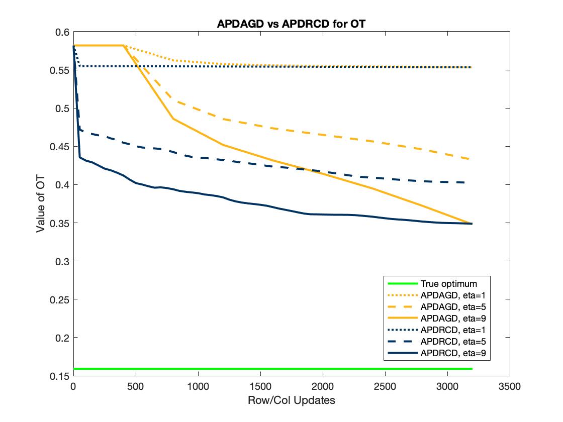
C.1 APDGCD algorithm with synthetic images

The generation of synthetic images as well as the evaluation metrics are similar to those in Section 4.1. We respectively present in Figure 4, Figure 5 and Figure 6 the comparisons between APDGCD algorithm versus APDAGD, APDAMD and APDRCD algorithms.

According to Figure 4, Figure 5 and Figure 6, the APDGCD algorithm enjoys better performance than the APDAGD, APDAMD and also the APDRCD algorithms in terms of the iteration numbers in terms of both the evaluation metrics. Besides, at the same number of iteration number, the APDGCD algorithm achieves even faster decrements than other three algorithms with regard to both the distance to polytope and the value of OT metrics during the computing process. This is beneficial in practice for easier tuning and smaller error when the update number is limited.

C.2 APDGCD algorithm with MNIST images

We present comparisons between APDGCD algorithm versus APDAGD, APDAMD, and APDRCD algorithms in Figure 7 with MNIST images.

According to Figure 7, the APDGCD algorithm enjoys better performance than the APDAGD, APDAMD and also the APDRCD algorithms in terms of the iteration numbers in terms of both the evaluation metrics. Furthermore, the convergence of the APDGCD algorithm is faster than other three algorithms with regard to both the distance to polytope and the value of OT metrics during the computing process when the number of iterations are small. This is beneficial in practice for easier tuning and smaller error when the total update number is limited.

C.3 APDRCD algorithm with larger synthetic image datasets and CIFAR10

In this section, we provide further experiments on the APDRCD algorithm on larger syntheric image datasets and CIFAR10 dataset. Results are included in Figure 8, Figure 9 and Figure 10. First, we provided results on the comparisons of APDRCD with APDAGD, APDAMD algorithms on larger synthetic datasets, with $n=30*30$ and $n=50*50$. We also provided the results on the CIFAR10 dataset. For each comparison, we provide the plots of the error of the dual variable versus the number of updates; and the error of the dual variable versus CPUtime (CPU: 3.1 GHz Intel Core i7) per iteration. The supplementary experiments show that APDRCD is more stable and achieve faster convergence in both number of row/col updates of the dual variables, and CPU time/iteration. The experimental setup are the same as the previous experiments except the change of dataset, hence omitted here.

References

• Altschuler et al. (2017) J. Altschuler, J. Weed, and P. Rigollet. Near-linear time approximation algorithms for optimal transport via Sinkhorn iteration. In NIPS, pages 1964–1974, 2017.
• Arjovsky et al. (2017) M. Arjovsky, S. Chintala, and L. Bottou. Wasserstein generative adversarial networks. In ICML, pages 214–223, 2017.
• Combettes and Pesquet (2012) P. L. Combettes and J. C. Pesquet. Primal-dual splitting algorithm for solving inclusions with mixtures of composite, Lipschitzian, and parallel-sum type monotone operators. Set-Valued and Variational Analysis, 20(2):307–330, 2012.
• Courty et al. (2017) N. Courty, R. Flamary, D. Tuia, and A. Rakotomamonjy. Optimal transport for domain adaptation. IEEE Transactions on Pattern Analysis and Machine Intelligence, 39(9):1853–1865, 2017.
• Cuturi (2013) M. Cuturi. Sinkhorn distances: lightspeed computation of optimal transport. In NIPS, pages 2292–2300, 2013.
• Cuturi and Doucet (2014) M. Cuturi and A. Doucet. Fast computation of Wasserstein barycenters. In ICML, pages 685–693, 2014.
• Dvurechenskii et al. (2018) P. Dvurechenskii, D. Dvinskikh, A. Gasnikov, C. Uribe, and A. Nedich. Decentralize and randomize: Faster algorithm for Wasserstein barycenters. In Advances in Neural Information Processing Systems, pages 10760–10770, 2018.
• Dvurechensky et al. (2018) P. Dvurechensky, A. Gasnikov, and A. Kroshnin. Computational optimal transport: Complexity by accelerated gradient descent is better than by Sinkhorn´s algorithm. In ICML, pages 1367–1376, 2018.
• Fercoq and Richtárik (2015) O. Fercoq and P. Richtárik. Accelerated, parallel, and proximal coordinate descent. SIAM Journal on Optimization, 25(4):1997–2023, 2015.
• Ho et al. (2019) N. Ho, V. Huynh, D. Phung, and M. I. Jordan. Probabilistic multilevel clustering via composite transportation fistance. AISTATS, 2019.
• Kalantari et al. (2008) B. Kalantari, I. Lari, F. Ricca, and B. Simeone. On the complexity of general matrix scaling and entropy minimization via the RAS algorithm. Mathematical Programming, 112(2):371–401, 2008.
• Kantorovich (1942) L. V. Kantorovich. On the translocation of masses. In Dokl. Akad. Nauk. USSR (NS), volume 37, pages 199–201, 1942.
• Knight (2008) P. A. Knight. The Sinkhorn–Knopp algorithm: Convergence and applications. SIAM Journal on Matrix Analysis and Applications, 30(1):261–275, 2008.
• Lee and Sidford (2014) Y. T. Lee and A. Sidford. Path finding methods for linear programming: Solving linear programs in O~~𝑂\widetilde{O}(sqrt(rank)) iterations and faster algorithms for maximum flow. In FOCS, pages 424–433. IEEE, 2014.
• Lin et al. (2018) T. Lin, Z. Hu, and X. Guo. Sparsemax and relaxed Wasserstein for topic sparsity. ArXiv Preprint: 1810.09079, 2018.
• Lin et al. (2019) T. Lin, N. Ho, and M. I. Jordan. On efficient optimal transport: An analysis of greedy and accelerated mirror descent algorithms. ArXiv Preprint arXiv:1901.06482, 2019.
• Nesterov (2012) Y. Nesterov. Efficiency of coordinate descent methods on huge-scale optimization problems. SIAM Journal on Optimization, 22(2):341–362, 2012.
• Nguyen (2013) X. Nguyen. Convergence of latent mixing measures in finite and infinite mixture models. Annals of Statistics, 4(1):370–400, 2013.
• Nguyen (2016) X. Nguyen. Borrowing strength in hierarchical Bayes: Posterior concentration of the Dirichlet base measure. Bernoulli, 22(3):1535–1571, 2016.
• Pele and Werman (2009) O. Pele and M. Werman. Fast and robust earth mover’s distance. In ICCV. IEEE, 2009.
• Richtárik and Takáč (2016) P. Richtárik and M. Takáč. Parallel coordinate descent methods for big data optimization. Mathematical Programming, 156(1-2):433–484, 2016.
• Rigollet and Weed (2019) P. Rigollet and J. Weed. Uncoupled isotonic regression via minimum Wasserstein deconvolution. Information and Inference: A Journal of the IMA, 8(4):691–717, 2019.
• Sinkhorn (1974) R. Sinkhorn. Diagonal equivalence to matrices with prescribed row and column sums. Proceedings of the American Mathematical Society, 45(2):195–198, 1974.
• Srivastava et al. (2015) S. Srivastava, V. Cevher, Q. Dinh, and D. Dunson. WASP: Scalable Bayes via barycenters of subset posteriors. In AISTATS, pages 912–920, 2015.
• Srivastava et al. (2018) S. Srivastava, C. Li, and D. Dunson. Scalable Bayes via barycenter in Wasserstein space. Journal of Machine Learning Research, 19(8):1–35, 2018.
• Tolstikhin et al. (2018) I. Tolstikhin, O. Bousquet, S. Gelly, and B. Schoelkopf. Wasserstein auto-encoders. In ICLR, 2018.
• Wainwright et al. (2005) M. J. Wainwright, T. S. Jaakkola, and A. S. Willsky. Map estimation via agreement on trees: Message-passing and linear programming. IEEE Transactions on Information Theory, 51(11):3697–3717, 2005.