Bayesian Optimization with Approximate Set Kernels

Abstract

We propose a practical Bayesian optimization method over sets, to minimize a black-box function that takes a set as a single input. Because set inputs are permutation-invariant, traditional Gaussian process-based Bayesian optimization strategies which assume vector inputs can fall short. To address this, we develop a Bayesian optimization method with set kernel that is used to build surrogate functions. This kernel accumulates similarity over set elements to enforce permutation-invariance, but this comes at a greater computational cost. To reduce this burden, we propose two key components: (i) a more efficient approximate set kernel which is still positive-definite and is an unbiased estimator of the true set kernel with upper-bounded variance in terms of the number of subsamples, (ii) a constrained acquisition function optimization over sets, which uses symmetry of the feasible region that defines a set input. Finally, we present several numerical experiments which demonstrate that our method outperforms other methods.

1 Introduction

Bayesian optimization is an effective method to optimize an expensive black-box function. It has proven useful in several applications, including hyperparameter optimization [36, 21], neural architecture search [43, 24], material design [11, 18], and synthetic gene design [16]. Classic Bayesian optimization assumes a search region ${\mathcal{X}}\subset{\mathbb{R}}^{d}$ and a black-box function $f$ evaluated in the presence of additive noise $\epsilon$, i.e., $y=f({\mathbf{x}})+\epsilon$ for ${\mathbf{x}}\in{\mathcal{X}}$.

Unlike this standard Bayesian optimization formulation, we assume that a search region is ${{\mathcal{X}}_{{\textrm{set}}}}=\{\{{\mathbf{x}}_{1},\ldots,{\mathbf{x}}_{m}\}\;|\;{\mathbf{x}}_{i}\in{\mathcal{X}}\subset{\mathbb{R}}^{d}\}$ for a fixed positive integer $m$. Thus, for ${\mathbf{X}}\in{{\mathcal{X}}_{{\textrm{set}}}}$, $f$ would take in a set containing $m$ elements, all of length $d$, and return a noisy function value $y$:

$$y=f\left({\mathbf{X}}\right)+\epsilon.$$ (1)

Our motivating example comes from the soft $k$-means clustering algorithm over a dataset ${\mathcal{P}}=\{{\mathbf{p}}_{1},\ldots,{\mathbf{p}}_{N}\}$; in particular, we aim to find the optimal initialization of such an algorithm. The objective function for this problem is a squared loss function which takes in the cluster initialization points $\{{\mathbf{x}}_{1},\ldots,{\mathbf{x}}_{k}\}$ and returns the weighted distance between the points in ${\mathcal{P}}$ and the converged cluster centers $\{{\mathbf{c}}_{1},\ldots,{\mathbf{c}}_{k}\}$. See [28] for more details.

Some previous research has attempted to build Gaussian process (GP) models on set data. [13] proposes a method over discrete sets using stationary kernels over the first Wasserstein distance between two sets, though the power set of fixed discrete sets as domain space is not our interest. However, this method needs the complexity ${\mathcal{O}}(n^{2}m^{3}d)$ to compute a covariance matrix with respect to $n$ sets. Moreover, since it only considers stationary kernels, GP regression is restricted to a form that cannot express non-stationary models [30].

Therefore, we instead adapt and augment a strategy proposed in [14] involving the creation of a specific set kernel. This set kernel uses a kernel defined on the elements ${\mathbf{x}}\in{\mathbb{R}}^{d}$ of the sets to build up its own sense of covariance between sets. In turn, then, it can be directly used to build surrogate functions through GP regression, which can power the Bayesian optimization strategy, by Lemma 1.

A key contribution of this article is the development of a computationally efficient approximation to this set kernel. Given $n$ total observed function values, the cost of constructing the matrix required for fitting the GP is ${\mathcal{O}}(n^{2}m^{2}d)$ where $m\geq n$ (see the complexity analysis in Section 3.3). The approximate set kernel proposed in this work uses random subsampling to reduce the computational cost to ${\mathcal{O}}(n^{2}L^{2}d)$ for $L<m$ while still producing an unbiased estimate of the expected value of the true kernel.

Another primary contribution is a constrained acquisition function optimization over set inputs. The next query set to observe is found by optimizing the acquisition function defined on a set ${\mathbf{X}}\in{{\mathcal{X}}_{{\textrm{set}}}}$. Using the symmetry of the space, this function can be efficiently optimized with a rejection sampling. Furthermore, we provide a theoretical analysis on cumulative regret bounds of our framework, which guarantees the convergence quality in terms of iterations.

2 Background

In this section, we briefly introduce previous studies, notations, and related work necessary to understand our algorithm.

2.1 Bayesian Optimization

Bayesian optimization seeks to minimize an unknown function $f$ which is expensive to evaluate, ${\mathbf{x}}^{\star}=\operatornamewithlimits{\arg\min}_{{\mathbf{x}}\in{\mathcal{X}}}f({\mathbf{x}})$, where ${\mathcal{X}}\subset{\mathbb{R}}^{d}$ is a compact space. It is a sequential optimization strategy which, at each iteration, performs the following three computations:

1. Using the $n$ data presently available, $\{({\mathbf{x}}_{i},y_{i})\}$ for $i\in[n]$, build a probabilistic surrogate model $s_{n}$ meant to approximate $f$.

2. Using the surrogate model $s_{n}$, compute an acquisition function $a_{n}$, which represents the utility of next acquiring data at some new point ${\mathbf{x}}$.

3. Observe $y_{n+1}$ from a true function $f$ at the location ${\mathbf{x}}_{n+1}=\operatornamewithlimits{\arg\max}_{{\mathbf{x}}\in{\mathcal{X}}}a_{n}({\mathbf{x}})$.

After exhausting a predefined budget $T$, Bayesian optimization returns the best point, ${\mathbf{x}}^{\dagger}$, that has the minimum observation. The benefit of this process is that the optimization of the expensive function $f$ has been replaced by the optimization of much cheaper and better understood acquisition functions $a_{n}$.

In this paper, we use GP regression [33] to produce the surrogate function $s_{n}$; from $s_{n}$, we use the Gaussian process upper confidence bound (GP-UCB) criterion [37]: $a_{n}({\mathbf{x}})=-\mu_{n}({\mathbf{x}})+\beta_{n}\sigma_{n}({\mathbf{x}})$, where $\mu_{n}(\cdot)$ and $\sigma_{n}^{2}(\cdot)$ are posterior mean and variance functions computed by $s_{n}$, and $\beta_{n}$ is a trade-off hyperparameter for exploration and exploitation at iteration $n$. See [3, 35, 10] for the details.

2.2 Set Kernel

We introduce the notation required for performing kernel approximation of functions on sets. A set of $m$ vectors is denoted as ${\mathbf{X}}=\{{\mathbf{x}}_{1},\ldots,{\mathbf{x}}_{m}\}$ , where ${\mathbf{x}}_{i}$ is in a compact space ${\mathcal{X}}\subset{\mathbb{R}}^{d}$. In a collection of $n$ such sets (as will occur in the Bayesian optimization setting), the $k$th set would be denoted ${\mathbf{X}}^{(k)}=\{{\mathbf{x}}_{1}^{(k)},\ldots,{\mathbf{x}}_{m}^{(k)}\}$. Note that we are restricting all sets to be of the same size $|{\mathbf{X}}^{(k)}|=m$.

To build a GP surrogate, we require a prior belief of the covariance between elements in ${{\mathcal{X}}_{{\textrm{set}}}}=\{\{{\mathbf{x}}_{1},\ldots,{\mathbf{x}}_{m}\}\;|\;{\mathbf{x}}_{i}\in{\mathcal{X}}\subset{\mathbb{R}}^{d}\}$. This belief is imposed in the form of a positive-definite kernel ${k_{{\textrm{set}}}}:{{\mathcal{X}}_{{\textrm{set}}}}\times{{\mathcal{X}}_{{\textrm{set}}}}\to{\mathbb{R}}$; see [34, 8] for more discussion on approximation with kernels. In addition to the symmetry ${k_{{\textrm{set}}}}({\mathbf{X}}^{(i)},{\mathbf{X}}^{(j)})={k_{{\textrm{set}}}}({\mathbf{X}}^{(j)},{\mathbf{X}}^{(i)})$ required in standard kernel settings, kernels on sets require an additional property: the ordering of elements in ${\mathbf{X}}$ should be immaterial (since sets have no inherent ordering).

Given an empirical approximation of the kernel mean ${\boldsymbol{\mu}}_{{\mathbf{X}}}\approx|{\mathbf{X}}|^{-1}\sum_{i=1}^{|{\mathbf{X}}|}\phi({\mathbf{x}}_{i})$, where $\phi$ is a feature map ${\mathbb{R}}^{d}\to{\mathbb{R}}^{d^{\prime}}$ and $d^{\prime}$ is a dimensionality of projected space by $\phi$, a set kernel [14, 29] is defined as

$${k_{{\textrm{set}}}}\left({\mathbf{X}}^{(1)},{\mathbf{X}}^{(2)}\right)=\left\langle{\boldsymbol{\mu}}_{{\mathbf{X}}^{(1)}},{\boldsymbol{\mu}}_{{\mathbf{X}}^{(2)}}\right\rangle=\frac{1}{|{\mathbf{X}}^{(1)}||{\mathbf{X}}^{(2)}|}\sum_{i=1}^{|{\mathbf{X}}^{(1)}|}\sum_{j=1}^{|{\mathbf{X}}^{(2)}|}k\left({\mathbf{x}}_{i}^{(1)},{\mathbf{x}}_{j}^{(2)}\right),$$ (2)

where $k({\mathbf{x}}_{i},{\mathbf{x}}_{j})=\langle\phi({\mathbf{x}}_{i}),\phi({\mathbf{x}}_{j})\rangle=\phi({\mathbf{x}}_{i})^{\top}\phi({\mathbf{x}}_{j})$. Here, $k:{\mathcal{X}}\times{\mathcal{X}}\to{\mathbb{R}}$ is a positive-definite kernel defined to measure the covariance between the $d$-dimensional elements of the sets (e.g., a squared exponential or Matérn kernel). The kernel (2) arises when comparing a class of functions on different probability measures with the intent of understanding if the measures might be equal [17].

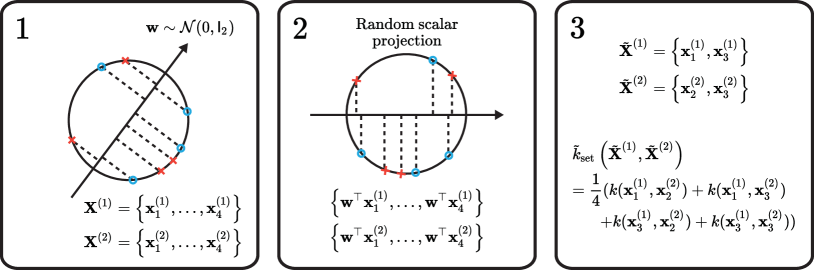
Figure 1: Illustration that shows how to select $L$ instances from sets, which originally have $m$ instances. In this example, $m=4$ and $L=2$. (Phase 1) Two set inputs are projected onto a vector that is randomly drawn from the standard Gaussian distribution. The points that have same color belong to same set (e.g., blue and red). (Phase 2) The location of the projections onto the line determines the order of the instances. (Phase 3) Using the order of instances, two instances uniformly sampled are selected and they are used to compute the approximate set kernel value.

2.3 Related Work

Although it has been raised in different interests, meta-learning approaches dealt with set inputs are promising in a machine learning community, because they can generalize distinct tasks with meta-learners [7, 41, 9, 12]. In particular, they propose feed-forward neural networks which take permutation-invariant and variable-length inputs: they have the goal of obtaining features derived from the sets with which to input to a standard (meta-)learning routine. Since they consider modeling of set structure, they are related to our work, but they are interested in their own specific examples such as point cloud classification, few-shot learning, and image completion.

In Bayesian optimization literature, [13] suggests a method to find a set that produces a global minimum with respect to discrete sets, each of which is an element of power set of entire set. This approach solves the problem related to set structure using the first Wasserstein distance over sets. However, for the reason why the time complexity of the first Wasserstein distance is ${\mathcal{O}}(n^{2}m^{3}d)$, they assume a small cardinality of sets and discrete search space for the global optimization method. Furthermore, their method restricts the number of iterations for optimizing an acquisition function, since the number of iterations should increase exponentially due to the curse of dimensionality. This implies that finding the global optimum of acquisition function is hard to achieve.

Compared to [13], we consider continuous domain space which implies an acquired set is composed of any instances in a compact space ${\mathcal{X}}$. We thus freely use off-the-shelf global optimization method or local optimization method [35] with relatively large number of instances in sets. In addition, its structure of kernel is $k_{\textrm{st}}(d({\mathbf{X}}^{(1)},{\mathbf{X}}^{(2)}))$ where $k_{\textrm{st}}(\cdot)$ is a stationary kernel [15] and $d(\cdot,\cdot)$ is a distance function over two sets (e.g., in [13] the first Wasserstein distance). Using the method proposed in Section 3, a non-stationary kernel might be considered in modeling a surrogate function.

Recently, [4] solves a similar set optimization problem using Bayesian optimization with deep embedding kernels. Compared to our method, it employs a kernel over RKHS embeddings as a kernel for set inputs, and shows its strict positive definiteness.

3 Proposed Method

We first propose and analyze an approximation to the set kernel (2) for GP regression in this section. Then, we present a Bayesian optimization framework over sets, by introducing our Bayesian optimization with approximate set kernels and a constrained optimization method for finding the next set to evaluate.

In order for (2) to be a viable kernel of a GP regression, it must be positive-definite. To discuss this topic, we denote a list of $n$ sets with the notation ${\mathfrak{X}}=[{\mathbf{X}}^{(1)},\ldots,{\mathbf{X}}^{(n)}]\in{{\mathcal{X}}_{{\textrm{set}}}}^{n}$; in this notation, the order of the entries matters.

Lemma 1.

Suppose we have a list ${\mathfrak{X}}$ which contains distinct sets ${\mathbf{X}}^{(i)}$ for $i\in[n]$. We define the matrix ${\mathsf{K}}\in{\mathbb{R}}^{n\times n}$ as

$$({\mathsf{K}})_{ij}={k_{{\textrm{set}}}}\left({\mathbf{X}}^{(i)},{\mathbf{X}}^{(j)}\right),$$ (3)

for ${k_{{\textrm{set}}}}$ defined with a chosen inner kernel $k$ as in (2). Then, ${\mathsf{K}}$ is a symmetric positive-semidefinite matrix if $k$ is a symmetric positive-definite kernel.

This proof appears in [20, Lemma 1], and is also discussed in [14].

3.1 Approximation of the Set Kernel

Computing (3) requires pairwise comparisons between all sets present in ${\mathfrak{X}}$, which has computational complexity ${\mathcal{O}}(n^{2}m^{2}d)$. To alleviate this cost, we propose to approximate (2) with

$${\tilde{k}_{{\textrm{set}}}}\left({\mathbf{X}}^{(1)},{\mathbf{X}}^{(2)};\pi,{\mathbf{w}},L\right)={k_{{\textrm{set}}}}\left({\tilde{{\mathbf{X}}}}^{(1)},{\tilde{{\mathbf{X}}}}^{(2)}\right),$$ (4)

where $\pi:[m]\to[m]$, ${\mathbf{w}}\in{\mathbb{R}}^{d}$ and $L\in{\mathbb{Z}}_{+}$ and ${\tilde{{\mathbf{X}}}}^{(i)}$ is a subset of ${\mathbf{X}}^{(i)}$ which is defined by those three quantities (we omit explicitly listing them in ${\tilde{{\mathbf{X}}}}^{(i)}$ to ease the notation).

The goal of the approximation strategy is to convert from ${\mathbf{X}}^{(i)}$ (of size $m$) to ${\tilde{{\mathbf{X}}}}^{(i)}$ (of size $L$) in a consistent fashion during all the ${\tilde{k}_{{\textrm{set}}}}$ computations comprising ${\mathsf{K}}$. As shown in Fig. 1, we accomplish this in two steps:

1. Use a randomly generated vector ${\mathbf{w}}$ to impose an (arbitrary) ordering of the elements of all sets ${\mathbf{X}}^{(i)}$, and

2. Randomly permute the indices $[m]$ via a function $\pi$.

These random strategies are defined once before computing the ${\mathsf{K}}$ matrix, and then used consistently throughout the entire computation.

Algorithm 1 Forming the ${\tilde{{\mathsf{K}}}}$ approximation to ${\mathsf{K}}$

0:  A list of sets ${\mathfrak{X}}=[{\mathbf{X}}^{(1)},\ldots,{\mathbf{X}}^{(n)}]$, $L\in{\mathbb{Z}}_{+}$.

0:  A matrix ${\tilde{{\mathsf{K}}}}$.

1:  Draw a random vector ${\mathbf{w}}$ from ${\mathcal{N}}(0,{\mathsf{I}}_{d})$.

2:  Create a random permutation of the integers $[m]$ with which to define $\pi$.

3:  Using ${\mathbf{w}}$, assign the ordering of elements in ${\mathbf{X}}^{(i)}$ according to (5).

4:  Using $\pi$, determine the subsets ${\tilde{{\mathbf{X}}}}^{(i)}$ as selected according to (6).

5:  Using these subsets and (4), populate the matrix with values:

$$({\tilde{{\mathsf{K}}}})_{ij}={\tilde{k}_{{\textrm{set}}}}({\mathbf{X}}^{(i)},{\mathbf{X}}^{(j)};{\mathbf{w}},\pi,L).$$

6:  return a computed matrix ${\tilde{{\mathsf{K}}}}$

To impose an ordering of the elements, we use a random scalar projection ${\mathbf{w}}\in{\mathbb{R}}^{d}$ such that the elements of ${\mathbf{w}}$ are drawn from the standard normal distribution. If the scalar projections of each ${\mathbf{x}}_{i}$ are computed, this produces the set of scalar values $\{{\mathbf{w}}^{\top}{\mathbf{x}}_{1},\ldots,{\mathbf{w}}^{\top}{\mathbf{x}}_{m}\}$, which can be sorted to generate an ordered list of

$$[\ell_{1},\ldots,\ell_{m}],\quad{\mathbf{w}}^{\top}{\mathbf{x}}_{\ell_{1}}\leq\ldots\leq{\mathbf{w}}^{\top}{\mathbf{x}}_{\ell_{m}},$$ (5)

for an ordering of distinct indices $\ell_{1},\ldots,\ell_{m}\in[m]$. Ties between ${\mathbf{w}}^{\top}{\mathbf{x}}_{i}$ values can be dealt with arbitrarily. The function $\pi$ then is simply a random bijection of the integers $[m]$ onto themselves. Using this, we can sample $L$ vectors from ${\mathbf{X}}^{(i)}$:

$${\tilde{{\mathbf{X}}}}^{(i)}=\{{\mathbf{x}}_{\ell_{j}}\;|\;\ell_{j}=\pi(j)\ \ \textrm{for}\ \ j\in[L]\}.$$ (6)

This process, given ${\mathbf{w}}$, $\pi$, and $L$, is sufficient for computing ${k_{{\textrm{set}}}}$, as presented in Algorithm 1.

3.2 Properties of the Approximation

The covariance matrix for this approximation of the set kernel, which we denote by $({\tilde{{\mathsf{K}}}})_{ij}={\tilde{k}_{{\textrm{set}}}}({\mathbf{X}}^{(i)},{\mathbf{X}}^{(j)};{\mathbf{w}},\pi,L)$, should approximate the full version of covariance matrix, ${\mathsf{K}}$ from (3). Because of the random structure introduced in Section 3.1, the matrix ${\tilde{{\mathsf{K}}}}$ will be random. This will be addressed in Theorem 1, but for now, ${\tilde{{\mathsf{K}}}}$ represents a single realization of that random variable, not the random variable itself. To be viable, this approximation must satisfy the following requirements:

Property 1.

The approximation satisfies pairwise symmetry:

$${\tilde{k}_{{\textrm{set}}}}\left({\mathbf{X}}^{(i)},{\mathbf{X}}^{(j)};{\mathbf{w}},\pi,L\right)={\tilde{k}_{{\textrm{set}}}}\left({\mathbf{X}}^{(j)},{\mathbf{X}}^{(i)};{\mathbf{w}},\pi,L\right).$$ (7)

Since ${\tilde{{\mathbf{X}}}}^{(i)}$ is uniquely defined given ${\mathbf{w}},\pi,L$, this simplifies to ${k_{{\textrm{set}}}}({\tilde{{\mathbf{X}}}}^{(i)},{\tilde{{\mathbf{X}}}}^{(j)})={k_{{\textrm{set}}}}({\tilde{{\mathbf{X}}}}^{(j)},{\tilde{{\mathbf{X}}}}^{(i)})$, which is true because ${k_{{\textrm{set}}}}$ is symmetric.

Property 2.

The “ordering” of the elements in the sets ${\mathbf{X}}^{(i)},{\mathbf{X}}^{(j)}$ should not matter when computing ${\tilde{k}_{{\textrm{set}}}}$. Indeed, because (5) enforces ordering based on ${\mathbf{w}}$, and not whatever arbitrary indexing is imposed in defining the elements of the set, the kernel will be permutation-invariant.

Property 3.

The kernel approximation (4) reduces to computing ${k_{{\textrm{set}}}}$ on a lower cardinality version of the data (with $L$ elements selected from $m$). Because ${k_{{\textrm{set}}}}$ is positive-definite on these $L$-element sets, we know that ${\tilde{k}_{{\textrm{set}}}}$ is also positive-definite.

Property 4.

Since the approximation method aims to choose subsets of input sets, the computational cost becomes lower than the original formulation.

Missing from these four properties is a statement regarding the quality of the approximation. We address this in Theorem 1 and Theorem 2, though we first start by stating Lemma 2.

Lemma 2.

Suppose there are two sets ${\mathbf{X}},{\mathbf{Y}}\in{{\mathcal{X}}_{{\textrm{set}}}}$. Without loss of generality, let ${\mathbf{X}}^{(i)}$ and ${\mathbf{Y}}^{(j)}$ denote the $i$th and $j$th of ${\binom{m}{L}}$ possible subsets containing $L$ elements of ${\mathbf{X}}$ and ${\mathbf{Y}}$, respectively, in an arbitrary ordering. For $L\in[m]$,

$$\sum_{i=1}^{{\binom{m}{L}}}\!\sum_{j=1}^{{\binom{m}{L}}}\!\sum_{a=1}^{L}\!\sum_{b=1}^{L}{k({\bar{{\mathbf{x}}}}^{(i)}_{a},{\bar{{\mathbf{y}}}}^{(j)}_{b})}=\frac{L^{2}{\binom{m}{L}}^{2}}{m^{2}}\!\sum_{c=1}^{m}\!\sum_{d=1}^{m}{k({\mathbf{x}}_{c},{\mathbf{y}}_{d})},$$ (8)

where ${\bar{{\mathbf{x}}}}^{(i)}_{a}$ and ${\bar{{\mathbf{y}}}}^{(j)}_{b}$ are the $a$th and $b$th elements of ${\mathbf{X}}^{(i)}$ and ${\mathbf{Y}}^{(j)}$, respectively, in an arbitrary ordering.

Proof.

We can rewrite the original summation in a slightly more convoluted form, as

$$\sum_{i=1}^{{\binom{m}{L}}}\sum_{j=1}^{{\binom{m}{L}}}\sum_{a=1}^{L}\sum_{b=1}^{L}{k({\bar{{\mathbf{x}}}}^{(i)}_{a},{\bar{{\mathbf{y}}}}^{(j)}_{b})}$$

$$=\sum_{i=1}^{{\binom{m}{L}}}\sum_{j=1}^{{\binom{m}{L}}}\sum_{a=1}^{L}\sum_{b=1}^{L}\sum_{c=1}^{m}\sum_{d=1}^{m}k({\bar{{\mathbf{x}}}}^{(i)}_{a},{\bar{{\mathbf{y}}}}^{(j)}_{b})I_{{\bar{{\mathbf{x}}}}^{(i)}_{a},{\bar{{\mathbf{y}}}}^{(j)}_{b}}({\mathbf{x}}_{c},{\mathbf{y}}_{d})$$

$$=\sum_{c=1}^{m}\!\sum_{d=1}^{m}\!\left[\sum_{i=1}^{{\binom{m}{L}}}\!\sum_{j=1}^{{\binom{m}{L}}}\!\sum_{a=1}^{L}\!\sum_{b=1}^{L}k({\bar{{\mathbf{x}}}}^{(i)}_{a},{\bar{{\mathbf{y}}}}^{(j)}_{b})I_{{\bar{{\mathbf{x}}}}^{(i)}_{a},{\bar{{\mathbf{y}}}}^{(j)}_{b}}({\mathbf{x}}_{c},{\mathbf{y}}_{d})\right],$$ (9)

where $I_{{\bar{{\mathbf{x}}}}^{(i)}_{a},{\bar{{\mathbf{y}}}}^{(j)}_{b}}({\mathbf{x}}_{c},{\mathbf{x}}_{d})=1$ if ${\bar{{\mathbf{x}}}}^{(i)}_{a}={\mathbf{x}}_{c}$ and ${\bar{{\mathbf{y}}}}^{(j)}_{b}={\mathbf{y}}_{d}$, and 0 otherwise. As these are finite summations, they can be safely reordered.

The symmetry in the structure and evaluation of the summation implies that as each ${\mathbf{x}}_{c}$ quantity will be paired with each ${\mathbf{y}}_{d}$ quantity the same number of times. Therefore, we need only consider the number of times that these quantities appear.

We recognize that this summation follows a pattern related to Pascal’s triangle. Among the ${\binom{m}{L}}$ possible subsets ${\bar{{\mathbf{x}}}}$ of ${\mathbf{X}}$, only the fraction $L/m$ of those contain the quantity ${\mathbf{x}}_{c}$ for all $c\in[m]$ (irrespective of how that entry may be denoted in ${\bar{{\mathbf{x}}}}^{(i)}_{a}$ terminology). Because of the symmetry mentioned above, each of those ${\mathbf{x}}_{c}$ quantities is paired with each of the ${\mathbf{y}}_{d}$ quantities the same $\frac{L}{m}{\binom{m}{L}}$ number of times. This result implies that

$$\sum_{i=1}^{{\binom{m}{L}}}\sum_{j=1}^{{\binom{m}{L}}}\sum_{a=1}^{L}\sum_{b=1}^{L}k({\bar{{\mathbf{x}}}}^{(i)}_{a},{\bar{{\mathbf{y}}}}^{(j)}_{b})I_{{\bar{{\mathbf{x}}}}^{(i)}_{a},{\bar{{\mathbf{y}}}}^{(j)}_{b}}({\mathbf{x}}_{c},{\mathbf{y}}_{d})=\frac{L^{2}{\binom{m}{L}}^{2}}{m^{2}}k({\mathbf{x}}_{c},{\mathbf{y}}_{d}),$$ (10)

where $I_{{\bar{{\mathbf{x}}}}^{(i)}_{a},{\bar{{\mathbf{y}}}}^{(j)}_{b}}({\mathbf{x}}_{c},{\mathbf{y}}_{d})=1$ if ${\bar{{\mathbf{x}}}}^{(i)}_{a}={\mathbf{x}}_{c}$ and ${\bar{{\mathbf{y}}}}^{(j)}_{b}={\mathbf{y}}_{d}$, and 0 otherwise. Substituting (10) into the bracketed quantity in (9) above completes the proof. ∎

We start by introducing the notation $W$ and $\Pi$ to be random variables such that $W\sim{\mathcal{N}}(0,{\mathsf{I}}_{d})$ and $\Pi$ is a uniformly random permutation of the integers between 1 and $m$. These are the distributions defining the ${\mathbf{w}}$ and $\pi$ quantities described above. With this, we note that ${\tilde{k}_{{\textrm{set}}}}({\mathbf{X}},{\mathbf{Y}};W,\Pi,L)$ is a random variable.

We also introduce the notation $\sigma_{L}({\mathbf{X}})$ to be the distribution of random subsets of ${\mathbf{X}}$ with $L$ elements selected without replacement, the outcome of the subset selection from Section 3.1. This notation allows us to write the quantities

$${\mathbb{E}}_{W,\Pi}[{\tilde{k}_{{\textrm{set}}}}({\mathbf{X}},{\mathbf{Y}};W,\Pi,L)] ={\mathbb{E}}_{{\bar{{\mathbf{X}}}},{\bar{{\mathbf{Y}}}}}[{k_{{\textrm{set}}}}({\bar{{\mathbf{X}}}},{\bar{{\mathbf{Y}}}})]\equiv{\mathbb{E}}[{k_{{\textrm{set}}}}({\bar{{\mathbf{X}}}},{\bar{{\mathbf{Y}}}})],$$ (11)

$${\textrm{Var}}_{W,\Pi}[{\tilde{k}_{{\textrm{set}}}}({\mathbf{X}},{\mathbf{Y}};W,\Pi,L)] ={\textrm{Var}}_{{\bar{{\mathbf{X}}}},{\bar{{\mathbf{Y}}}}}[{k_{{\textrm{set}}}}({\bar{{\mathbf{X}}}},{\bar{{\mathbf{Y}}}})]\equiv{\textrm{Var}}[{k_{{\textrm{set}}}}({\bar{{\mathbf{X}}}},{\bar{{\mathbf{Y}}}})],$$ (12)

for ${\bar{{\mathbf{X}}}}\sim\sigma_{L}({\mathbf{X}}),{\bar{{\mathbf{Y}}}}\sim\sigma_{L}({\mathbf{Y}})$. We have dropped the random variables from the expectation and variance definitions for ease of notation.

Theorem 1.

Suppose that we are given two sets ${\mathbf{X}},{\mathbf{Y}}\in{{\mathcal{X}}_{{\textrm{set}}}}$ and $L\in{\mathbb{Z}}_{+}$. Suppose, furthermore, that ${\mathbf{w}}$ and $\pi$ can be generated randomly as defined in Section 3.1 to form subsets ${\tilde{{\mathbf{X}}}}$ and ${\tilde{{\mathbf{Y}}}}$. The value of ${\tilde{k}_{{\textrm{set}}}}({\mathbf{X}},{\mathbf{Y}};{\mathbf{w}},\pi,L)$ is an unbiased estimator of the value of ${k_{{\textrm{set}}}}({\mathbf{X}},{\mathbf{Y}})$.

Proof.

Our goal is to show that ${\mathbb{E}}[{k_{{\textrm{set}}}}({\bar{{\mathbf{X}}}},{\bar{{\mathbf{Y}}}})]\!=\!{k_{{\textrm{set}}}}({\mathbf{X}},{\mathbf{Y}})$, where ${\mathbb{E}}[{k_{{\textrm{set}}}}({\bar{{\mathbf{X}}}},{\bar{{\mathbf{Y}}}})]$ is defined in (11).

We first introduce an extreme case: $L=m$. If $L=m$, the subsets we are constructing are the full sets, i.e., $\sigma_{m}({\mathbf{X}})$ contains only one element, ${\mathbf{X}}$. Thus, ${\tilde{k}_{{\textrm{set}}}}({\mathbf{X}},{\mathbf{Y}};W,\Pi,m)={k_{{\textrm{set}}}}({\mathbf{X}},{\mathbf{Y}})$ is not a random variable.

For $1\leq L<m$, we compute this expected value from the definition (with some abuse of notation):

$${\mathbb{E}}[{k_{{\textrm{set}}}}({\bar{{\mathbf{X}}}},{\bar{{\mathbf{Y}}}})]=\sum_{{\bar{{\mathbf{X}}}},{\bar{{\mathbf{Y}}}}}{k_{{\textrm{set}}}}({\bar{{\mathbf{X}}}},{\bar{{\mathbf{Y}}}})p({\bar{{\mathbf{X}}}},{\bar{{\mathbf{Y}}}}).$$ (13)

There are ${\binom{m}{L}}$ subsets, all of which could be indexed (arbitrarily) as ${\bar{{\mathbf{X}}}}^{(i)}$ for $1\leq i\leq{\binom{m}{L}}$. The probability mass function is uniform across all subsets, meaning that $p({\bar{{\mathbf{X}}}}={\bar{{\mathbf{X}}}}^{(i)},{\bar{{\mathbf{Y}}}}={\bar{{\mathbf{Y}}}}^{(j)})=1/\binom{m}{L}^{2}$. Using this, we know

$${\mathbb{E}}[{k_{{\textrm{set}}}}({\bar{{\mathbf{X}}}},{\bar{{\mathbf{Y}}}})]=\sum_{i=1}^{{\binom{m}{L}}}\sum_{j=1}^{{\binom{m}{L}}}{k_{{\textrm{set}}}}({\bar{{\mathbf{X}}}}^{(i)},{\bar{{\mathbf{Y}}}}^{(j)})\frac{1}{{\binom{m}{L}}^{2}}.$$ (14)

We apply (2) to see that

$${k_{{\textrm{set}}}}({\bar{{\mathbf{X}}}}^{(i)},{\bar{{\mathbf{Y}}}}^{(j)})=\frac{1}{L^{2}}\sum_{a=1}^{L}\sum_{b=1}^{L}k({\bar{{\mathbf{x}}}}^{(i)}_{a},{\bar{{\mathbf{y}}}}^{(j)}_{b}),$$ (15)

following the notational conventions used above. The expectation involves four nested summations,

$${\mathbb{E}}[{k_{{\textrm{set}}}}({\bar{{\mathbf{X}}}},{\bar{{\mathbf{Y}}}})]=\frac{1}{L^{2}{\binom{m}{L}}^{2}}\sum_{i=1}^{{\binom{m}{L}}}\sum_{j=1}^{{\binom{m}{L}}}\sum_{a=1}^{L}\sum_{b=1}^{L}k({\bar{{\mathbf{x}}}}^{(i)}_{a},{\bar{{\mathbf{y}}}}^{(j)}_{b}).$$ (16)

We utilize Lemma 2 to rewrite this as

$${\mathbb{E}}[{k_{{\textrm{set}}}}({\bar{{\mathbf{X}}}},{\bar{{\mathbf{Y}}}})]=\frac{1}{L^{2}{\binom{m}{L}}^{2}}\frac{L^{2}{\binom{m}{L}}^{2}}{m^{2}}\sum_{c=1}^{m}\sum_{d=1}^{m}{k({\mathbf{x}}_{c},{\mathbf{y}}_{d})}=\frac{1}{m^{2}}\sum_{c=1}^{m}\sum_{d=1}^{m}{k({\mathbf{x}}_{c},{\mathbf{y}}_{d})}.$$ (17)

∎

Theorem 2.

Under the same conditions as in Theorem 1, suppose that $k({\mathbf{x}},{\mathbf{x}}^{\prime})\geq 0$ for all ${\mathbf{x}},{\mathbf{x}}^{\prime}\in{\mathcal{X}}$. The variance of ${\tilde{k}_{{\textrm{set}}}}({\mathbf{X}},{\mathbf{Y}};{\mathbf{w}},\pi,L)$ is bounded by a function of $m$, $L$ and ${k_{{\textrm{set}}}}({\mathbf{X}},{\mathbf{Y}})$:

$${\textrm{Var}}\left[{\tilde{k}_{{\textrm{set}}}}({\mathbf{X}},{\mathbf{Y}};{\mathbf{w}},\pi,L)\right]\leq\left(\frac{m^{4}}{L^{4}}-1\right){k_{{\textrm{set}}}}({\mathbf{X}},{\mathbf{Y}})^{2}.$$ (18)

Proof.

The variance of ${k_{{\textrm{set}}}}({\bar{{\mathbf{X}}}},{\bar{{\mathbf{Y}}}})$, defined in (12), is computed as

$${\textrm{Var}}\left[{k_{{\textrm{set}}}}({\bar{{\mathbf{X}}}},{\bar{{\mathbf{Y}}}})\right] ={\mathbb{E}}\left[\left({k_{{\textrm{set}}}}({\bar{{\mathbf{X}}}},{\bar{{\mathbf{Y}}}})-{\mathbb{E}}\left[{k_{{\textrm{set}}}}({\bar{{\mathbf{X}}}},{\bar{{\mathbf{Y}}}})\right]\right)^{2}\right]$$

$$={\mathbb{E}}\left[{k_{{\textrm{set}}}}({\bar{{\mathbf{X}}}},{\bar{{\mathbf{Y}}}})^{2}\right]+{k_{{\textrm{set}}}}({\mathbf{X}},{\mathbf{Y}})^{2}-2{k_{{\textrm{set}}}}({\mathbf{X}},{\mathbf{Y}}){\mathbb{E}}\left[{k_{{\textrm{set}}}}({\bar{{\mathbf{X}}}},{\bar{{\mathbf{Y}}}})\right]$$

$$={\mathbb{E}}\left[{k_{{\textrm{set}}}}({\bar{{\mathbf{X}}}},{\bar{{\mathbf{Y}}}})^{2}\right]-{k_{{\textrm{set}}}}({\mathbf{X}},{\mathbf{Y}})^{2},$$ (19)

where Theorem 1 is invoked to produce the final line. Using (14) and (15), we can express the first term of (19) as

$${\mathbb{E}}\left[{k_{{\textrm{set}}}}({\bar{{\mathbf{X}}}},{\bar{{\mathbf{Y}}}})^{2}\right]=\sum_{i=1}^{{\binom{m}{L}}}\sum_{j=1}^{{\binom{m}{L}}}\left(\frac{1}{L^{2}}\sum_{a=1}^{L}\sum_{b=1}^{L}k({\bar{{\mathbf{x}}}}_{a}^{(i)},{\bar{{\mathbf{x}}}}_{b}^{(j)})\right)^{2}\frac{1}{{\binom{m}{L}}^{2}}.$$ (20)

At this point, we invoke the fact that $k({\mathbf{x}},{\mathbf{x}}^{\prime})\geq 0$ to state

$$0\leq\sum_{a=1}^{L}\sum_{b=1}^{L}k({\bar{{\mathbf{x}}}}_{a}^{(i)},{\bar{{\mathbf{x}}}}_{b}^{(j)})\leq\sum_{a=1}^{m}\sum_{b=1}^{m}k({\mathbf{x}}_{a},{\mathbf{x}}_{b}),$$ (21)

which is true because the summation to $m$ terms contains all of the elements in the summation to $L$ terms, as well as other (nonnegative) elements. Using this, we can bound (20) by

$${\mathbb{E}}\left[{k_{{\textrm{set}}}}({\bar{{\mathbf{X}}}},{\bar{{\mathbf{Y}}}})^{2}\right] \leq\sum_{i=1}^{{\binom{m}{L}}}\sum_{j=1}^{{\binom{m}{L}}}\left(\frac{1}{L^{2}}\sum_{a=1}^{m}\sum_{b=1}^{m}k({\mathbf{x}}_{a},{\mathbf{x}}_{b})\right)^{2}\frac{1}{{\binom{m}{L}}^{2}}$$

$$=\frac{m^{4}}{{\binom{m}{L}}^{2}L^{4}}\sum_{i=1}^{{\binom{m}{L}}}\sum_{j=1}^{{\binom{m}{L}}}\left(\frac{1}{m^{2}}\sum_{a=1}^{m}\sum_{b=1}^{m}k({\mathbf{x}}_{a},{\mathbf{x}}_{b})\right)^{2}$$

$$=\frac{m^{4}}{{\binom{m}{L}}^{2}L^{4}}{\binom{m}{L}}^{2}{k_{{\textrm{set}}}}({\mathbf{X}},{\mathbf{Y}})^{2}=\frac{m^{4}}{L^{4}}{k_{{\textrm{set}}}}({\mathbf{X}},{\mathbf{Y}})^{2}.$$ (22)

Therefore, with (22), (19) can be written as

$${\textrm{Var}}\left[{k_{{\textrm{set}}}}({\bar{{\mathbf{X}}}},{\bar{{\mathbf{Y}}}})\right]\leq\frac{m^{4}}{L^{4}}{k_{{\textrm{set}}}}({\mathbf{X}},{\mathbf{Y}})^{2}-{k_{{\textrm{set}}}}({\mathbf{X}},{\mathbf{Y}})^{2}=\left(\frac{m^{4}}{L^{4}}-1\right){k_{{\textrm{set}}}}({\mathbf{X}},{\mathbf{Y}})^{2},$$ (23)

which concludes this proof. ∎

The restriction $k({\mathbf{x}},{\mathbf{x}}^{\prime})\geq 0$ is satisfied by many standard covariance kernels (such as the Gaussian, the Matérn family and the multiquadric) as well as some more interesting choices (such as the Wendland or Wu families of compactly supported kernels). It does, however, exclude some oscillatory kernels such as the Poisson kernel as well as kernels defined implicitly which may have an oscillatory behavior. More discussion on different types of kernels and their properties can be found in the kernel literature [8].

By Theorem 2, we can naturally infer the fact that the upper bound of the variance decreases quickly, as $L$ is close to $m$.

3.3 Bayesian Optimization over Sets

For Bayesian optimization over ${{\mathcal{X}}_{{\textrm{set}}}}$, the goal is to identify the set ${\mathbf{X}}\in{{\mathcal{X}}_{{\textrm{set}}}}$ such that a given function $f:{{\mathcal{X}}_{{\textrm{set}}}}\to{\mathbb{R}}$ is minimized. As shown in Algorithm 2, Bayesian optimization over sets follows similar steps as laid out in Section 2, except that it involves the space of set inputs and requires a surrogate function on ${{\mathcal{X}}_{{\textrm{set}}}}$. As we have already indicated, we plan to use a GP surrogate function, with prior covariance defined either with (2) or (4) and a Matérn 5/2 inner kernel $k$.

A GP model requires computation on the order of ${\mathcal{O}}(n^{3})$ at the $n$th step of the Bayesian optimization because the ${\mathsf{K}}$ matrix must be inverted. Compared to the complexity for computing a full version of the set kernel ${\mathcal{O}}(n^{2}m^{2}d)$, the complexity of computing the inverse is smaller if roughly $m\geq n$ (that is, computing the matrix can be as costly or more costly than inverting it). Because Bayesian optimization is efficient sampling-based global optimization, $n$ is small and the situation $m\geq n$ is reasonable. Therefore, the computation reduction by our approximation can be effective in reducing complexity of all steps for Bayesian optimization over sets.

In addition, since the Cholesky decomposition, instead of matrix inverse is widely used to compute posterior mean and variance functions [33], the time complexity for inverting a covariance matrix can be reduced. But still, if $m$ is relatively large, our approximation is effective. In this paper, we compute GP surrogate using the Cholesky decomposition. See the effects of $L$ in Section 4.1.

Algorithm 2 Bayesian Optimization over Sets

0:  A domain ${{\mathcal{X}}_{{\textrm{set}}}}$, a function $f:{{\mathcal{X}}_{{\textrm{set}}}}\to{\mathbb{R}}$, a budget $T\in{\mathbb{Z}}_{+}$.

0:  Best acquired set ${\mathbf{X}}^{\dagger}$.

1:  Choose an initial point ${\mathbf{X}}^{(1)}$ randomly from ${{\mathcal{X}}_{{\textrm{set}}}}$ and evaluate $y_{1}=f({\mathbf{X}}^{(1)})+\epsilon_{1}$.

2:  for $k$ from $1$ to $T-1$ do

3:     Fit the surrogate model $s_{k}$ to all data $\{({\mathbf{X}}^{(i)},y_{i})\}_{i=1}^{k}$.

4:     Compute the acquisition function $a_{k}$ from $s_{k}$.

5:     Identify ${\mathbf{X}}^{(k+1)}=\operatornamewithlimits{\arg\max}_{{\mathbf{X}}\in{{\mathcal{X}}_{{\textrm{set}}}}}a_{k}({\mathbf{X}})$.

6:     Evaluate $y_{k+1}=f({\mathbf{X}}^{(k+1)})+\epsilon_{k+1}$.

7:  end for

8:  return ${\mathbf{X}}^{\dagger}={\mathbf{X}}^{(i)}$ if $y_{i}=\max_{j\in[T]}y_{j}$

3.4 Acquisition Function Optimization over Sets

An acquisition function optimization step is one of the primary steps in Bayesian optimization, because this step is for finding an acquired example, which exhibits the highest potential of the global optimum. Compared to generic vector-input Bayesian optimization methods, our Bayesian optimization over sets needs to find a query set ${\mathbf{X}}$ on ${{\mathcal{X}}_{{\textrm{set}}}}$, optimizing the acquisition function over sets.

Since $m$ is fixed when we find ${\mathbf{X}}$, off-the-shelf optimization methods such as L-BFGS-B [27], DIRECT [23], and CMA-ES [19] can be employed where a set is treated as a concatenated vector. However, because of the symmetry of the space ${{\mathcal{X}}_{{\textrm{set}}}}$, these common optimization methods search more of the space than is required. For instance, if we optimize the function on $\{1,2,3\}$, we would not need to consider such the sets $\{1,3,2\},\{2,1,3\},\ldots,\{3,2,1\}$. Therefore, we suggest a constrained acquisition function optimization with rejection sampling algorithm. The sample complexity of this method decreases by a factor of $m!$.

First of all, we sample all instances of the sets to initialize acquisition function optimization from uniform distribution. By the rejection sampling, some of the sets sampled are rejected if each of them is located outside of the symmetric region. The optimization method (i.e., CMA-ES) finds the optimal set of the acquisition function, starting from those initial sets selected from the aforementioned step. In the optimization step, our optimization strategy forces every optimization result to locate in the symmetric search space. Finally, we pick the best one among the converged sets as the next set to observe.

3.5 Regret Analysis

To produce a regret bound on Bayesian optimization with our approximation as well as one of Bayesian optimization with the set kernel, we follow the framework to prove the regret bounds of the multi-armed bandit-like acquisition function in [37]. To simplify the analysis, we discuss only the Matérn kernel for $\nu>2$ as a base kernel for GP.

Inspired by [25], we assume that our objective function $f$ can be expressed as a summation of functions over instances and they can be collected to a function that can take a single vector with the i.i.d. property of instances in a set:

$$f({\mathbf{X}})=\frac{1}{m}\sum_{i=1}^{m}g({\mathbf{x}}_{i})=h([{\mathbf{x}}_{1},\ldots,{\mathbf{x}}_{m}]),$$ (24)

which implies that $h$ can take $md$-dimensional concatenated inputs. Thus, we can state our Bayesian optimization with the set kernel follows the cumulative regret bound proposed by [37] and [25]. Given $T$ available sets $\{{\mathbf{X}}^{(1)},\ldots,{\mathbf{X}}^{(T)}\}$, let $\delta\in(0,1)$ and trade-off hyperparameter for GP-UCB $\beta_{t}\in{\mathcal{O}}(md\log t)$. A cumulative regret bound $R_{T}$ is

$$R_{T}={\mathcal{O}}(md2^{d}T^{\frac{\nu+d(d+1)}{2\nu+d(d+1)}}),$$ (25)

with the probability at least $1-\delta$, under the mild assumptions: (i) ${k_{{\textrm{set}}}}({\mathbf{X}},{\mathbf{X}}^{\prime})\leq 1$; (ii) the bounded reproducing kernel Hilbert space (RKHS) norm $\|f\|_{{k_{{\textrm{set}}}}}<b$ where $b>0$. Moreover, ${\tilde{k}_{{\textrm{set}}}}({\mathbf{X}},{\mathbf{X}}^{\prime};{\mathbf{w}},\pi,L)\leq 1$ and $\|f\|_{{\tilde{k}_{{\textrm{set}}}}}<b$ are naturally satisfied by their definitions.

By Theorem 1 and Theorem 2, we can define Corollary 1, which is related to the aforementioned regret bound.

Corollary 1.

Suppose that $0<\delta\ll 1$. $R_{T}^{(L)}$ is a cumulative regret computed by the approximate set kernel with $L$ of $m$ instances in each set. By Theorem 1 and Theorem 2, ${\mathbb{E}}_{L}[R_{T}^{(L)}]=R_{T}$, is satisfied with the probability at least $1-\delta$.

Proof.

Since our approximation is an unbiased estimator of original set kernel ${k_{{\textrm{set}}}}$ with bounded variance as discussed in Theorem 1 and Theorem 2, the expectation of cumulative regrets with the approximation is equal to $R_{T}$. ∎

4 Experiments

In this section, we present various experimental results, to show unique applications of our method as well as the motivating problems. First, we conduct our method on the experiments regarding set kernel approximation and constrained acquisition function optimization, in order to represent the effectiveness of our proposed method. Then, we optimize two synthetic functions and clustering algorithm initialization, which take a set as an input. Finally, we present the experimental results on active nearest neighbor search for point clouds.

We define the application-agnostic baseline methods, Vector and Split:

Vector A standard Bayesian optimization is performed over a $md$-dimensional space where, at the $n$th step, the available data ${\mathfrak{X}}_{n}\in{{\mathcal{X}}_{{\textrm{set}}}}^{n}$ is vectorized to $[{\mathbf{x}}_{1},\ldots,{\mathbf{x}}_{n}]$ for ${\mathbf{x}}_{i}\in{\mathbb{R}}^{md}$ with associated function values. At each step, the vectorized next location ${\mathbf{x}}_{n+1}$ is converted into a set ${\mathbf{X}}_{n+1}$.

Split Individual Bayesian optimization strategies are executed on the $m$ components comprising ${\mathcal{X}}$. At the $n$th step, the available data ${\mathfrak{X}}_{n}\in{{\mathcal{X}}_{{\textrm{set}}}}^{n}$ is decomposed into $m$ sets of data, the $i$th of which consists of $[{\mathbf{x}}^{(i)}_{1},\ldots,{\mathbf{x}}^{(i)}_{n}]$ with associated data. The $m$ vectors produced during each step of the optimization are then collected to form ${\mathbf{X}}_{n+1}$ at which to evaluate $f$.

For Vector and Split baselines, to satisfy the permutation-invariance property, we determine the order of elements in a set as the ascending order by the $l^{2}$ norm of the elements.

We use Gaussian process regression [33] with a set kernel or Matérn 5/2 kernel as a surrogate function. Because computing the inverse of covariance matrix needs heavy computations, we employ the Cholesky decomposition instead [33]. For the experiments with set kernel, Matérn 5/2 kernel is used as a base kernel. All Gaussian process regression models are optimized by marginal likelihood maximization with the BFGS optimizer, to find kernel hyperparameters. We use Gaussian process upper confidence bound criterion [37] as an acquisition function for all experiments. CMA-ES [19] and its constrained version are applied in optimizing the acquisition function. Furthermore, five initial points are given to start a single round of Bayesian optimization. Unless otherwise specified, most of experiments are repeated 10 times. For the results on execution time, all the results include the time consumed in evaluating a true function. All results are run via CPU computations. All implementations which will be released as open source project are written in Python. Thanks to [31], we use scikit-learn in many parts of our implementations.

4.1 Set Kernel Approximation

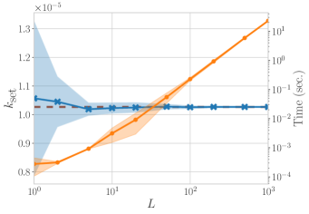
(a) Kernel approximation

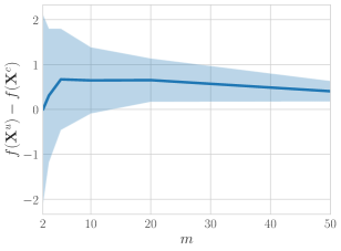
(b) Constrained optimization

Figure 2: Results on the effects of $L$ for set kernels and constrained optimization for acquisition functions. The mean and standard deviation of each quantity are plotted, computed over 10 trials. (left) The lines with x and o indicate kernel values and consumed times, respectively. The dashed line is the true set kernel value. (right) ${\mathbf{X}}^{u}$ and ${\mathbf{X}}^{c}$ are the acquired sets obtained by the acquisition function optimization w/o and w/ constraints, respectively.

Table 1: The effects of $L$ for set kernels. All settings follow the settings in Fig. 2(a). The numerical results are rounded to the three decimals, to show the effects precisely.

$L$	${k_{{\textrm{set}}}}$	Time (sec.)
$1$	$1.057\times 10^{-5}\pm 1.387\times 10^{-6}$	$(2.776\pm 0.877)\times 10^{-4}$
$2$	$1.045\times 10^{-5}\pm 4.512\times 10^{-7}$	$(3.131\pm 0.118)\times 10^{-4}$
$5$	$1.019\times 10^{-5}\pm 1.168\times 10^{-7}$	$(9.283\pm 0.089)\times 10^{-4}$
$10$	$1.023\times 10^{-5}\pm 9.980\times 10^{-8}$	$(3.133\pm 0.822)\times 10^{-3}$
$20$	$1.025\times 10^{-5}\pm 9.305\times 10^{-8}$	$(9.150\pm 3.169)\times 10^{-3}$
$50$	$1.028\times 10^{-5}\pm 4.955\times 10^{-8}$	$(5.487\pm 1.075)\times 10^{-2}$
$100$	$1.026\times 10^{-5}\pm 3.030\times 10^{-8}$	$(2.282\pm 0.134)\times 10^{-1}$
$200$	$1.027\times 10^{-5}\pm 1.961\times 10^{-8}$	$(9.253\pm 0.490)\times 10^{-1}$
$500$	$1.027\times 10^{-5}\pm 1.372\times 10^{-8}$	$(5.887\pm 0.159)\times 10^{0}$
$1000(=m)$	$1.027\times 10^{-5}$	$(2.295\pm 0.027)\times 10^{1}$

We study the effect of $L$ for the set kernels. Using a set generated from the standard normal distribution, which has 1,000 $50$-dimensional instances, we observe the effects of $L$ as shown in Fig. 2(a). ${k_{{\textrm{set}}}}$ converges to the true value as $L$ increases, and the variance of ${k_{{\textrm{set}}}}$ value is large when $L$ is small, as discussed in Section 3.2. Moreover, the consumed time increases as $L$ increases. We use Matérn 5/2 kernel as a base kernel. Table 1 shows the effects of $L$ for set kernels. As $L$ increases, ${k_{{\textrm{set}}}}$ value is converged to the true value and execution time increases.

4.2 Constrained Acquisition Function Optimization

We demonstrate the effects of the constrained acquisition function optimization, compared to the vanilla optimization method that concatenates a set to a single vector. In this paper, we use CMA-ES [19] as an acquisition function optimization method, which is widely used in Bayesian optimization [2, 38]. As we mentioned in Section 3.4, the constrained CMA-ES is more sample-efficient than the vanilla CMA-ES. Fig. 2(b) (i.e., a minimization problem) represents that the function values determined by the constrained method are always smaller than the values by the unconstrained method, because we fix the number of initial samples (i.e., 5). Moreover, the variance of them decreases, as $m$ is large. For this experiment, we measure the acquisition performance where 20 fixed historical observations are given, and Synthetic 1 described in Section 4.3 is used. Note that the kernel approximation is not applied.

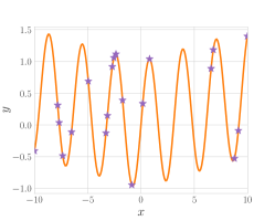
(a) Vector

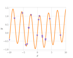
(b) Split

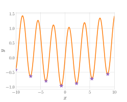
(c) Ours (w/o approx.)

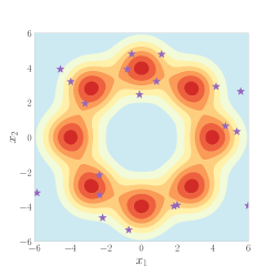
(d) Vector

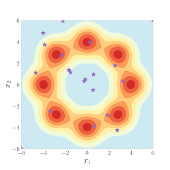
(e) Split

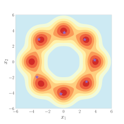
(f) Ours (w/o approx.)

Figure 3: Examples of one of the best acquisition results (i.e., purple stars indicate instances in the acquired set) via Vector, Split, and Ours (w/o approximation). For Synthetic 1 (first row) and Synthetic 2 (second row), $m$ is set to $20$.

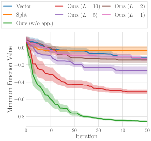
(a) Synthetic 1

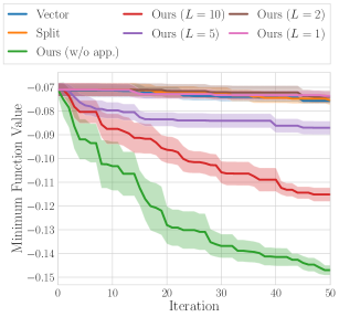
(b) Synthetic 2

Figure 4: Results on optimizing two synthetic functions. As presented in Fig. 3, $m$ is set to $20$. All experiments are repeated 10 times.

4.3 Synthetic Functions

We test two synthetic functions to show Bayesian optimization over sets is a valid approach to find an optimal set that minimizes an objective function $f:{{\mathcal{X}}_{{\textrm{set}}}}\to{\mathbb{R}}$. In each setting, there is an auxiliary function $g:{\mathcal{X}}\to{\mathbb{R}}$, and $f$ is defined as $f({\mathbf{X}})=\frac{1}{m}\sum_{i=1}^{m}g({\mathbf{x}}_{i})$. The $g$ functions are designed to be multi-modal, giving the opportunity for the set ${\mathbf{X}}$ to contain ${\mathbf{x}}_{i}$ values from each of the modes in the domain. Additionally, as is expected, $f$ is permutation invariant (any ordering imposed on the elements of ${\mathbf{x}}$ is immaterial).

Synthetic 1 We consider $d=1$, $m=20$ and choose $g$ to be a simple periodic function:

$$g({\mathbf{x}})=\sin(2\|{\mathbf{x}}\|_{2})+|0.05\|{\mathbf{x}}\|_{2}|.$$ (26)

Synthetic 2 We consider $d=2$, $m=20$ and a $g$ function which is the sum of probability density functions:

$$g({\mathbf{x}})=-\sum_{i=1}^{8}p({\mathbf{x}};\mu_{i},\Sigma_{i}),$$ (27)

where $p$ is the normal density function with $\mu_{i}$ depicted in Fig. 3 and $\Sigma_{i}={\mathsf{I}}_{2}$.

As shown in Fig. 3, both of these functions have a clear multimodal structure, allowing for optimal sets to contain points which are clustered in a single local minima or to be spread out through the domain in several local minima. Fig. 4 shows that Vector and Split strategies have difficulty optimizing the functions. On the other hand, our proposed method finds optimal outcomes more effectively. We study the impact of $L$ when optimizing these two synthetic functions; a smaller $L$ should yield faster computations, but also a worse approximation ${\tilde{{\mathsf{K}}}}$ to the true ${\mathsf{K}}$ matrix (when $L=m$).

Table 2 represents a convergence quality and its execution time for the synthetic functions defined in this work. As expected, the execution time decreases as $L$ decreases.

4.4 Clustering Algorithm Initialization

Table 2: Convergence quality and its execution time on two synthetic functions where $m=20$. All settings follow the settings in Fig. 3 and Fig. 4.

	Synthetic 1		Synthetic 2
$L$	Minimum	Time ($10^{3}$ sec.)	Minimum	Time ($10^{3}$ sec.)
$1$	$-0.133\pm 0.052$	$5.682\pm 0.279$	$-0.074\pm 0.004$	$6.468\pm 0.130$
$2$	$-0.146\pm 0.071$	$8.003\pm 0.156$	$-0.074\pm 0.005$	$9.768\pm 0.136$
$5$	$-0.266\pm 0.090$	$16.299\pm 0.253$	$-0.087\pm 0.006$	$20.451\pm 0.033$
$10$	$-0.516\pm 0.052$	$31.010\pm 0.810$	$-0.115\pm 0.006$	$40.099\pm 0.085$
$20(=m)$	$-0.858\pm 0.019$	$91.589\pm 2.339$	$-0.147\pm 0.004$	$85.266\pm 0.297$

We initialize clustering algorithms for dataset ${\mathcal{P}}=[{\mathbf{p}}_{1},\ldots,{\mathbf{p}}_{N}]$ with Bayesian optimization over sets. For these experiments, we add four additional baselines for clustering algorithms:

Random This baseline randomly draws $k$ points from a compact space $\subset{\mathbb{R}}^{d}$.

Data This baseline randomly samples $k$ points from a dataset ${\mathcal{P}}$. It is widely used in initializing a clustering algorithm.

($k$-means only) $k$-means++ [1] This is a method for $k$-means clustering with the intuition that spreading out initial cluster centers is better than the Data baseline.

(GMM only) $k$-means This baseline sets initial cluster centers as the results of $k$-means clustering.

To fairly compare the baselines to our methods, the baselines are trained by the whole datasets without splitting. To compare with the baselines fairly, Random, Data, $k$-means++ [1], $k$-means are run 1,000 times. In Bayesian optimization settings, we split a dataset to training (70%) and test (30%) datasets. After finding the converged cluster centers $\{{\mathbf{c}}_{1},\ldots,{\mathbf{c}}_{k}\}$ with training dataset, the adjusted Rand index (ARI) is computed by test dataset. The algorithms are optimized over $1-\textrm{ARI}$. All clustering models are implemented using scikit-learn [31].

We test two clustering algorithms for synthetic datasets: (i) $k$-means clustering and (ii) Gaussian mixture model (GMM). In addition, two real-world datasets are tested to initialize $k$-means clustering: (i) Handwritten Digits dataset [6] and (ii) NIPS Conference Papers dataset [32]. As shown in Fig. 5 and Fig. 6, our methods outperform other application-agnostic baselines as well as four baselines for clustering methods.

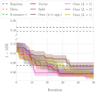
(a) $k$-means clustering

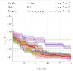
(b) Gaussian mixture model

Figure 5: Results on initializing clustering algorithms: $k$-means clustering and Gaussian mixture model for synthetic datasets.

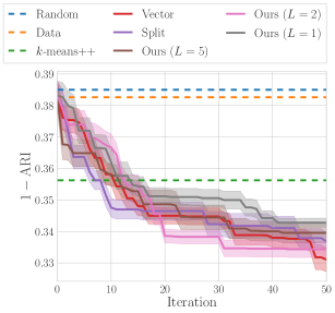
(a) Handwritten Digits

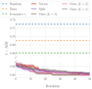
(b) NIPS Conference Papers

Figure 6: Results on initializing $k$-means clustering for Handwritten Digits and NIPS Conference Papers datasets.

Table 3: Convergence quality and its execution time on $k$-means clustering and Gaussian mixture model. All settings follow the settings in Fig. 5.

	$\boldsymbol{k}$-means clustering		Gaussian mixture model
$L$	$1-$ARI	Time ($10^{3}$ sec.)	$1-$ARI	Time ($10^{3}$ sec.)
$1$	$0.051\pm 0.024$	$3.140\pm 0.051$	$0.202\pm 0.011$	$2.364\pm 0.178$
$2$	$0.058\pm 0.030$	$5.034\pm 0.145$	$0.197\pm 0.038$	$3.873\pm 0.148$
$5$	$0.050\pm 0.022$	$13.891\pm 0.327$	$0.194\pm 0.033$	$13.105\pm 0.675$
$10(=m)$	$0.073\pm 0.038$	$45.527\pm 2.475$	$0.205\pm 0.030$	$49.134\pm 1.469$

Table 4: Convergence quality and its execution time on $k$-means clustering for Handwritten Digits and NIPS Conference Papers datasets. All settings follow the settings in Fig. 6.

	Handwritten Digits		NIPS Conference Papers
$L$	$1-$ARI	Time ($10^{3}$ sec.)	$1-$ARI	Time ($10^{3}$ sec.)
$1$	$0.343\pm 0.007$	$39.347\pm\,\ 6.533$	$0.621\pm 0.006$	$4.757\pm 0.138$
$2$	$0.334\pm 0.013$	$47.550\pm\,\ 1.832$	$0.620\pm 0.007$	$9.410\pm 0.260$
$5$	$0.340\pm 0.016$	$177.170\pm 43.063$	$0.620\pm 0.007$	$38.521\pm 1.551$

Synthetic Datasets We generate a dataset sampled from Gaussian distributions, where $N=500$, $d=5$, and $k=10$.

Real-World Datasets Two real-world datasets are tested: (i) Handwritten Digits dataset [6] and (ii) NIPS Conference Papers dataset [32]. Handwritten Digits dataset contains 0–9 digit images that can be expressed as $N=1797$, $d=64$, and $k=10$. NIPS Conference Papers dataset is composed of the papers published from 1987 to 2015. The features of each example are word frequencies, and this dataset can be expressed as $N=5811$, $d=11463$, and $k=20$. However, without any techniques for reducing the dimensionality, this dataset is hard to apply the clustering algorithm. We choose 200 dimensions in random when creating the dataset for these experiments, because producing the exact clusters for entire dimensions is not our interest in this paper.

Because the real-world datasets for clustering are difficult to specify truths, we determine truths as class labels for Handwritten Digits dataset [6] and clustering results via Ward hierarchical clustering [39] for NIPS Conference Papers dataset [32].

The function of interest in the $k$-means clustering setting is the converged clustering residual

$$k\textrm{-means}(\{{\mathbf{x}}_{1},\ldots,{\mathbf{x}}_{k}\})=\sum_{i=1}^{N}\sum_{j=1}^{k}w_{ij}\|{\mathbf{p}}_{i}-{\mathbf{c}}_{j}\|^{2}_{2},$$ (28)

where $\{{\mathbf{x}}_{1},\ldots,{\mathbf{x}}_{k}\}$ is the set of proposed initial cluster centers, $\{{\mathbf{c}}_{1},\ldots,{\mathbf{c}}_{k}\}$ is the set of converged cluster centers [28], and $w_{ij}$ are softmax values from the pairwise distances. Here, the fact that ${\mathbf{c}}_{j}$ is a function of ${\mathbf{X}}$ and ${\mathcal{P}}$ is omitted for notational simplicity. The set of converged cluster centers is determined through an iterative strategy which is highly dependent on the initial points ${\mathbf{X}}$ to converge to effective centers.

In contrast to $k$-means clustering, the GMM estimates parameters of Gaussian distributions and mixing parameters between the distributions. Because it is difficult to minimize negative log-likelihood of the observed data, we fit the GMM using expectation-maximization algorithm [5]. Similarly to $k$-means clustering, this requires initial guesses ${\mathbf{X}}$ to converge to cluster centers $\{\mathbf{c}_{1},\ldots,\mathbf{c}_{k}\}$.

Table 3 shows convergence qualities and their execution time on $k$-means clustering algorithm and GMM for synthetic datasets, and Table 4 represents the qualities and their execution for Handwritten Digits and NIPS Conference Papers datasets. Similar to Table 1, the computational cost increases as $L$ increases.

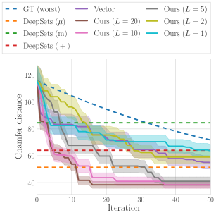
(a) 100 examples

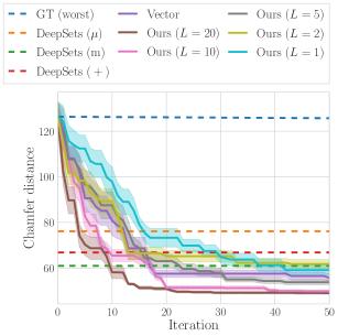
(b) Entire examples

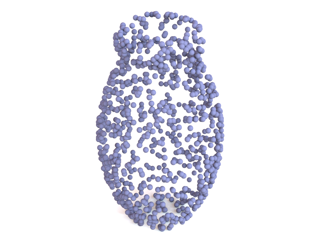
(c) Query 1

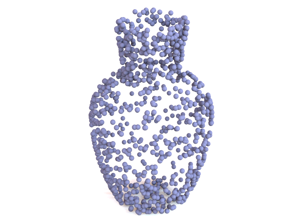
(d) NN 1

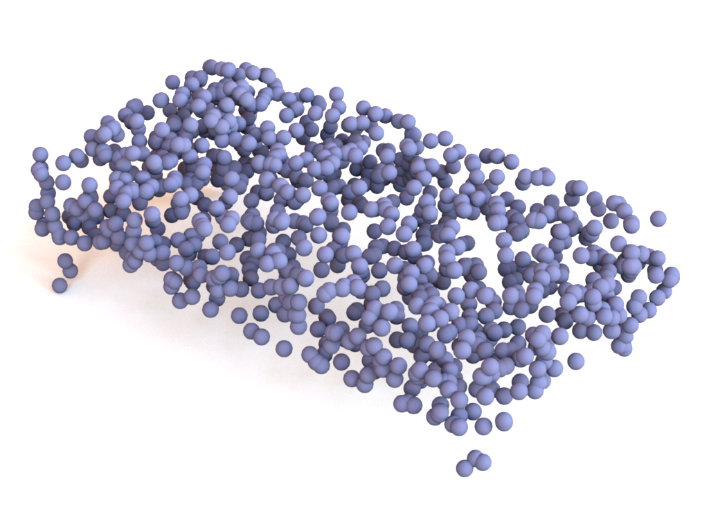
(e) Query 2

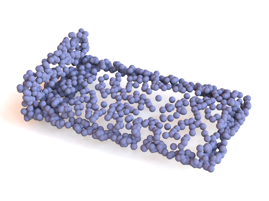
(f) NN 2

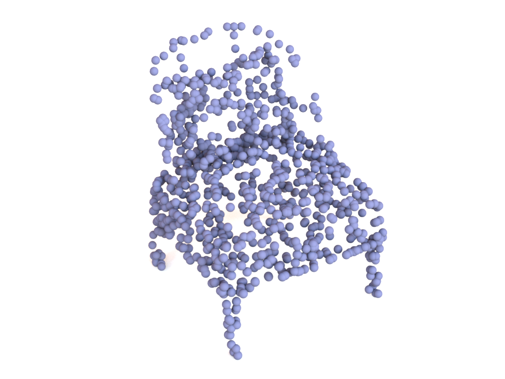
(g) Query 3

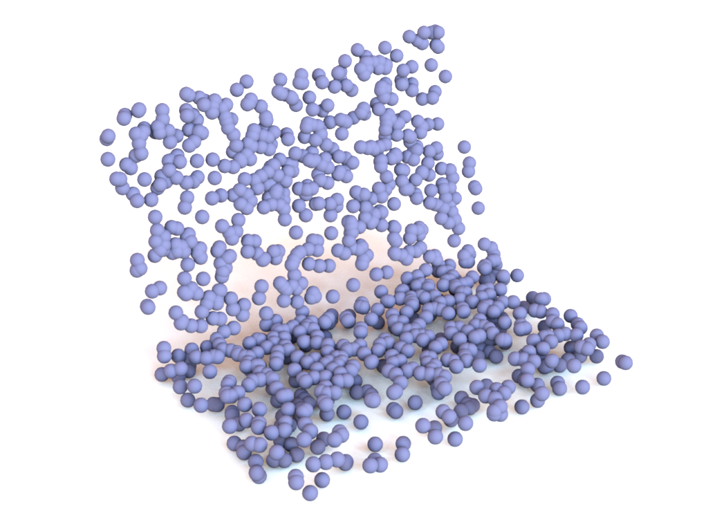
(h) NN 3

Figure 7: Nearest neighbor search results on ModelNet40 point clouds. GT and DeepSets (m) indicate the ground-truth and DeepSets (max), respectively. Query and NN pairs are the query and its nearest neighbor examples found by our method.

Table 5: Convergence quality and its execution time on nearest neighbor retrieval for ModelNet40 point clouds. All settings follow the settings in Fig. 7.

	100 examples		Entire examples
$L$	Chamfer distance	Time ($10^{3}$ sec.)	Chamfer distance	Time ($10^{3}$ sec.)
$1$	$63.720\pm 23.780$	$1.133\pm 0.049$	$59.095\pm 10.629$	$1.071\pm 0.067$
$2$	$59.079\pm 25.610$	$1.844\pm 0.109$	$61.783\pm 10.000$	$1.835\pm 0.094$
$5$	$41.072\pm 15.807$	$6.568\pm 0.485$	$53.820\pm\,\ 5.643$	$6.456\pm 0.372$
$10$	$38.422\pm 12.807$	$21.156\pm 1.360$	$49.798\pm\,\ 3.121$	$23.482\pm 1.111$
$20$	$38.422\pm 12.807$	$104.330\pm 5.045$	$49.054\pm\,\ 2.614$	$97.179\pm 3.882$

4.5 Active Nearest Neighbor Search for Point Clouds

ModelNet40 dataset [40] contains 40 categories of 12,311 3D CAD models. Point cloud representation is obtained by sampling uniformly 1,024 points from the surface of each 3D model using Open3D [42]. Nearest neighbor search for point clouds requires large number of Chamfer distance calculations, which is a time-consuming task, in particular when the size of dataset is large. We employ our Bayesian optimization over sets to actively select a candidate whose Chamfer distance from the query is to be computed, while the linear scan requires the calculation of Chamfer distance from the query to every other data in the dataset:

$$d_{\textrm{Chamfer}}({\mathbf{X}},{\mathbf{Y}})=\sum_{{\mathbf{x}}\in{\mathbf{X}}}\min_{{\mathbf{y}}\in{\mathbf{Y}}}\|{\mathbf{x}}-{\mathbf{y}}\|_{2}$$ (29)

where $|{\mathbf{X}}|=|{\mathbf{Y}}|=m$ and each element in ${\mathbf{X}}$ and ${\mathbf{Y}}$ is a three-dimensional real vector.

For this experiment, we use one oracle and three additional baselines:

Ground-truth (worst) It is the worst case to achieve the ground-truth. The best retrieval case is to find the ground-truth at once, and the usual case would be between the best and the worst.

DeepSets ($\mu$) / DeepSets (max) / DeepSets ($+$) These baselines are implemented to embed point clouds to a single vector using DeepSets [41], and measure $l^{2}$ distance between the embeddings. Because we can access to class information of ModelNet40 dataset [40], these neural networks can be trained to match the information. We use three fully-connected layers with batch normalization [22] as an instance-wise network, and four fully-connected layers with batch normalization as a network after aggregation. ReLU is employed as an activation function. The choice of global aggregation methods determines each baseline: (i) mean aggregation is $\mu$; (ii) max aggregation is max; and (iii) sum aggregation is $+$. Because retrieving 1-nearest neighbor with these methods is hard to obtain the nearest neighbor, we choose the nearest neighbor from 3-nearest neighbors to fairly compare with our methods.

Experiments with two different settings were carried out: (i) the size of point clouds is 100; (ii) full-size point clouds (the cardinality is 12,311). In the case of DeepSets, point clouds are embedded into a low-dimensional Euclidean space, so that Euclidean distance is used to search a nearest neighbor (i.e., approximate search). On the other hand, our method actively selects a candidate gradually in the point cloud dataset. The nearest neighbor determined by our method, given the query, is shown in Fig. 7. About 20 iterations of the procedure is required to achieve the better performance, compared to DeepSets (Fig. 7(a) and Fig. 7(b)).

4.6 Empirical Analysis on Computational Cost

The computational costs from Table 1 to Table 5 are presented as a function of $L$. These results are measured using a native implementation of set kernels written in Python. As mentioned in Section 3, the computational costs follow our expectation, which implies that the complexity for computing a covariance matrix over sets is the major computations in the overall procedure.

5 Conclusion

In this paper, we propose the Bayesian optimization method over sets, which takes a set as an input and produces a scalar output. Our method based on GP regression models a surrogate function using set-taking covariance functions, referred to as set kernel. We approximate the set kernel to the efficient positive-definite kernel that is an unbiased estimator of the original set kernel. To find a next set to observe, we employ a constrained acquisition function optimization using the symmetry of the feasible region defined over sets. Moreover, we provide a simple analysis on cumulative regret bounds of our methods. Our experimental results demonstrate our method can be used in some novel applications for Bayesian optimization.

Conflict of interest

The authors declare that they have no conflict of interest.

References

- [1] Arthur, D., Vassilvitskii, S.: k-means++: The advantages of careful seeding. In: Proceedings of the ACM-SIAM Symposium on Discrete Algorithms (SODA), pp. 1027–1035. New Orleans, Louisiana, USA (2007)
- [2] Bergstra, J., Bardenet, R., Bengio, Y., Kégl, B.: Algorithms for hyper-parameter optimization. In: Advances in Neural Information Processing Systems (NeurIPS), vol. 24, pp. 2546–2554. Granada, Spain (2011)
- [3] Brochu, E., Cora, V.M., de Freitas, N.: A tutorial on Bayesian optimization of expensive cost functions, with application to active user modeling and hierarchical reinforcement learning. arXiv preprint arXiv:1012.2599 (2010)
- [4] Buathong, P., Ginsbourger, D., Krityakierne, T.: Kernels over sets of finite sets using RKHS embeddings, with application to Bayesian (combinatorial) optimization. In: Proceedings of the International Conference on Artificial Intelligence and Statistics (AISTATS), pp. 2731–2741. Virtual (2020)
- [5] Dempster, A.P., Laird, N.M., Rubin, D.B.: Maximum likelihood from incomplete data via the EM algorithm. Journal of the Royal Statistical Society B 39, 1–38 (1977)
- [6] Dua, D., Graff, C.: UCI machine learning repository. http://archive.ics.uci.edu/ml (2019)
- [7] Edwards, H., Storkey, A.: Towards a neural statistician. In: Proceedings of the International Conference on Learning Representations (ICLR). Toulon, France (2017)
- [8] Fasshauer, G.E., McCourt, M.M.: Kernel-based Approximation Methods Using Matlab. World Scientific (2015)
- [9] Finn, C., Abbeel, P., Levine, S.: Model-agnostic meta-learning for fast adaptation of deep networks. In: Proceedings of the International Conference on Machine Learning (ICML), pp. 1126–1135. Sydney, Australia (2017)
- [10] Frazier, P.I.: A tutorial on Bayesian optimization. arXiv preprint arXiv:1807.02811 (2018)
- [11] Frazier, P.I., Wang, J.: Bayesian optimization for materials design. In: Information Science for Materials Discovery and Design, pp. 45–75. Springer (2016)
- [12] Garnelo, M., Rosenbaum, D., Maddison, C.J., Ramalho, T., Saxton, D., Shanahan, M., Teh, Y.W., Rezende, D.J., Eslami, S.M.A.: Conditional neural processes. In: Proceedings of the International Conference on Machine Learning (ICML), pp. 1690–1699. Stockholm, Sweden (2018)
- [13] Garnett, R., Osborne, M.A., Roberts, S.J.: Bayesian optimization for sensor set selection. In: ACM/IEEE International Conference on Information Processing in Sensor Networks (IPSN), pp. 209–219. Stockholm, Sweden (2010)
- [14] Gätner, T., Flach, P.A., Kowalczyk, A., Smola, A.J.: Multi-instance kernels. In: Proceedings of the International Conference on Machine Learning (ICML), pp. 179–186. Sydney, Australia (2002)
- [15] Genton, M.G.: Classes of kernels for machine learning: a statistics perspective. Journal of Machine Learning Research 2, 299–312 (2001)
- [16] González, J., Longworth, J., James, D.C., Lawrence, N.D.: Bayesian optimization for synthetic gene design. In: Neural Information Processing Systems Workshop on Bayesian Optimization (BayesOpt). Montreal, Quebec, Canada (2014)
- [17] Gretton, A., Borgwardt, K.M., Rasch, M.J., Schölkopf, B., Smola, A.J.: A kernel two-sample test. Journal of Machine Learning Research 13, 723–773 (2012)
- [18] Haghanifar, S., McCourt, M., Cheng, B., Wuenschell, J., Ohodnicki, P., Leu, P.W.: Creating glasswing butterfly-inspired durable antifogging superomniphobic supertransmissive, superclear nanostructured glass through Bayesian learning and optimization. Materials Horizons 6(8), 1632–1642 (2019)
- [19] Hansen, N.: The CMA evolution strategy: A tutorial. arXiv preprint arXiv:1604.00772 (2016)
- [20] Haussler, D.: Convolution kernels on discrete structures. Tech. rep., Department of Computer Science, University of California at Santa Cruz (1999)
- [21] Hutter, F., Hoos, H.H., Leyton-Brown, K.: Sequential model-based optimization for general algorithm configuration. In: Proceedings of the International Conference on Learning and Intelligent Optimization (LION), pp. 507–523. Rome, Italy (2011)
- [22] Ioffe, S., Szegedy, C.: Batch normalization: Accelerating deep network training by reducing internal covariate shift. In: Proceedings of the International Conference on Machine Learning (ICML), pp. 448–456. Lille, France (2015)
- [23] Jones, D.R., Perttunen, C.D., Stuckman, B.E.: Lipschitzian optimization without the Lipschitz constant. Journal of Optimization Theory and Applications 79(1), 157–181 (1993)
- [24] Kandasamy, K., Neiswanger, W., Schneider, J., Póczos, B., Xing, E.P.: Neural architecture search with Bayesian optimisation and optimal transport. In: Advances in Neural Information Processing Systems (NeurIPS), vol. 31, pp. 2016–2025. Montreal, Quebec, Canada (2018)
- [25] Kandasamy, K., Schneider, J., Póczos, B.: High dimensional Bayesian optimisation and bandits via additive models. In: Proceedings of the International Conference on Machine Learning (ICML), pp. 295–304. Lille, France (2015)
- [26] Kim, J., McCourt, M., You, T., Kim, S., Choi, S.: Bayesian optimization over sets. In: International Conference on Machine Learning Workshop on Automated Machine Learning (AutoML). Long Beach, California, USA (2019)
- [27] Liu, D.C., Nocedal, J.: On the limited memory BFGS method for large scale optimization. Mathematical Programming 45(3), 503–528 (1989)
- [28] Lloyd, S.P.: Least squares quantization in PCM. IEEE Transactions on Information Theory 28(2), 129–137 (1982)
- [29] Muandet, K., Fukumizu, K., Sriperumbudur, B., Schölkopf, B.: Kernel mean embedding of distributions: A review and beyond. Foundations and Trends® in Machine Learning 10(1-2), 1–141 (2017)
- [30] Paciorek, C.J., Schervish, M.J.: Nonstationary covariance functions for Gaussian process regression. In: Advances in Neural Information Processing Systems (NeurIPS), vol. 17, pp. 273–280. Vancouver, British Columbia, Canada (2004)
- [31] Pedregosa, F., Varoquaux, G., Gramfort, A., Michel, V., Thirion, B., Grisel, O., Blondel, M., Prettenhofer, P., Weiss, R., Dubourg, V., et al.: Scikit-learn: Machine learning in Python. Journal of Machine Learning Research 12, 2825–2830 (2011)
- [32] Perrone, V., Jenkins, P.A., Spano, D., Teh, Y.W.: Poisson random fields for dynamic feature models. Journal of Machine Learning Research 18, 1–45 (2017)
- [33] Rasmussen, C.E., Williams, C.K.I.: Gaussian Processes for Machine Learning. MIT Press (2006)
- [34] Schölkopf, B., Smola, A.J.: Learning with Kernels. MIT Press (2002)
- [35] Shahriari, B., Swersky, K., Wang, Z., Adams, R.P., de Freitas, N.: Taking the human out of the loop: A review of Bayesian optimization. Proceedings of the IEEE 104(1), 148–175 (2016)
- [36] Snoek, J., Larochelle, H., Adams, R.P.: Practical Bayesian optimization of machine learning algorithms. In: Advances in Neural Information Processing Systems (NeurIPS), vol. 25, pp. 2951–2959. Lake Tahoe, Nevada, USA (2012)
- [37] Srinivas, N., Krause, A., Kakade, S., Seeger, M.: Gaussian process optimization in the bandit setting: No regret and experimental design. In: Proceedings of the International Conference on Machine Learning (ICML), pp. 1015–1022. Haifa, Israel (2010)
- [38] Wang, Z., Shakibi, B., Jin, L., de Freitas, N.: Bayesian multi-scale optimistic optimization. In: Proceedings of the International Conference on Artificial Intelligence and Statistics (AISTATS), pp. 1005–1014. Reykjavik, Iceland (2014)
- [39] Ward, J.H.: Hierarchical grouping to optimize an objective function. Journal of the American Statistical Association 58(301), 236–244 (1963)
- [40] Wu, Z., Song, S., Khosla, A., Yu, F., Zhang, L., Tang, X., Xiao, J.: 3D ShapeNets: A deep representation for volumetric shapes. In: Proceedings of the IEEE International Conference on Computer Vision and Pattern Recognition (CVPR), pp. 1912–1920. Boston, Massachusetts, USA (2015)
- [41] Zaheer, M., Kottur, S., Ravanbakhsh, S., Poczos, B., Salakhutdinov, R.R., Smola, A.J.: Deep sets. In: Advances in Neural Information Processing Systems (NeurIPS), vol. 30, pp. 3391–3401. Long Beach, California, USA (2017)
- [42] Zhou, Q., Park, J., Koltun, V.: Open3D: A modern library for 3D data processing. arXiv preprint arXiv:1801.09847 (2018)
- [43] Zoph, B., Le, Q.V.: Neural architecture search with reinforcement learning. In: Proceedings of the International Conference on Learning Representations (ICLR). Toulon, France (2017)