A Smoothness Energy without Boundary Distortion for Curved Surfaces
Abstract.
Current quadratic smoothness energies for curved surfaces either exhibit distortions near the boundary due to zero Neumann boundary conditions, or they do not correctly account for intrinsic curvature, which leads to unnatural-looking behavior away from the boundary. This leads to an unfortunate trade-off: one can either have natural behavior in the interior, or a distortion-free result at the boundary, but not both. We introduce a generalized Hessian energy for curved surfaces, expressed in terms of the covariant one-form Dirichlet energy, the Gaussian curvature, and the exterior derivative. Energy minimizers solve the Laplace-Beltrami biharmonic equation, correctly accounting for intrinsic curvature, leading to natural-looking isolines. On the boundary, minimizers are as-linear-as-possible, which reduces the distortion of isolines at the boundary. We discretize the covariant one-form Dirichlet energy using Crouzeix-Raviart finite elements, arriving at a discrete formulation of the Hessian energy for applications on curved surfaces. We observe convergence of the discretization in our experiments.
1. Introduction
Smoothness energies are used as objective functions for optimization in geometry processing. A wide variety of applications exists: smoothness energies can be used to smooth data on surfaces, to denoise data, for scattered data interpolation, character animation, and much more. We are interested in quadratic smoothness energies formulated on triangle meshes.
It is desirable for a smoothing energy to have minimizers with isolines whose spacing does not vary much across the surface—the gradient of the function is sufficiently constant. When the gradient of the function is sufficiently constant, the function only changes very gradually, resulting in a smooth function. In the same vein, a good smoothing energy should have minimizers whose isolines are not distorted anywhere: their spacing is not influenced (on the interior) by the surface’s curvature, and they are not biased by the boundary of the surface—they behave locally as if the boundary were absent. Such behavior is relevant for applications where the boundary is not directly related to the actual problem that is being solved, e.g., when the boundary is an artificial result of faulty surface reconstruction resulting in a shape with many extraneous holes. One class of energies with the desired behavior in the interior are energies whose minimizers solve the biharmonic equation, the prototypical elliptic equation of order four. (Gazzola et al., 2010, viii). Such energies are pertinent as smoothness energies in computer graphics applications (Jacobson et al., 2010).
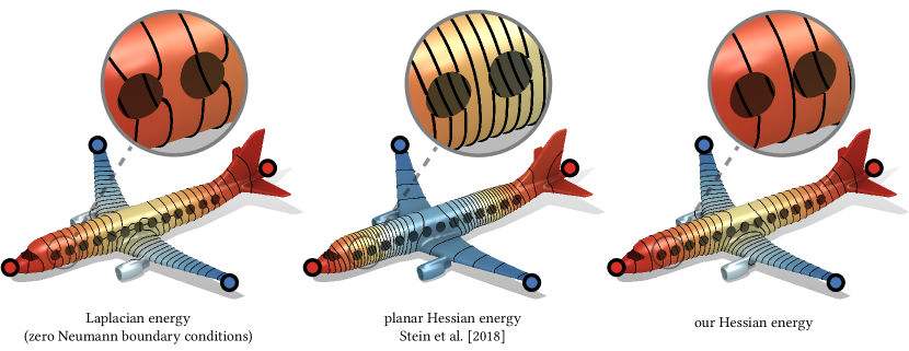
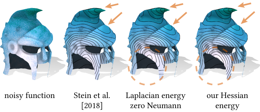
One such energy is the squared Laplacian energy—the squared Laplacian of a function integrated over the surface. We henceforth refer to the energy as simply the Laplacian energy. Its minimizers solve the biharmonic equation; as a result, they are very smooth, and their isolines behave well on curved surfaces, if the surfaces are closed. The energy’s most popular discretization, however, comes with zero Neumann boundary conditions. Thus, if a surface has boundaries, the minimizers are distorted near the boundary (see Figure 1), since at the boundary they are as-constant-as-possible.
The issue of boundary distortion is addressed by the Hessian energy of Stein et al. (2018). For planar domains, they provide an energy whose minimizers solve the biharmonic equation and are as-linear-as-possible at the boundary. These boundary conditions lead to decreased distortion. The Hessian energy of Stein et al. (2018), however, is only defined for subsets of the plane . Stein et al. (2018) offer a way to compute an energy for curved surfaces, but, as they point out, their approach does not account for the curvature of the surface correctly. The approach of Stein et al. (2018) does not solve the biharmonic equation on curved surfaces; this leads to global distortions in the isolines of the solution (see Figure 1).
Contributions
(1) Generalized Hessian energy.
We generalize the Hessian energy to accommodate curved surfaces. Our new Hessian energy is
| (1) |
where is the covariant derivative of differential forms, d is the exterior derivative, is the Gaussian curvature, and denotes the contraction of two operators in all indices that corresponds to (where the transpose takes the metric into account). This energy
-
•
corresponds to the Laplacian energy in the case of a domain without boundaries;
-
•
corresponds to the Hessian energy of Stein et al. (2018) for surfaces in , , where is the Hessian matrix of , and is the Frobenius norm of ;
-
•
has the as-linear-as-possible natural boundary conditions of the Hessian energy of Stein et al. (2018) for flat domains in . These boundary conditions lead to decreased distortion at the boundary.
Figure 1 shows how our Hessian energy manages to achieve the best of both worlds.
(2) Discretization.
We also introduce a discretization of this curved Hessian energy that uses Crouzeix-Raviart finite elements “under the hood”, but, after the energy matrix has been assembled, relies solely on piecewise linear hat functions. We observe convergence of the discretization for a wide variety of numerical experiments, given certain regularity conditions, and apply it to various smoothing and interpolation problems.
2. Related Work
This work extends Stein et al. (2018). They introduce a smoothness energy with higher-order boundary conditions whose minimizers are biased less by the shape of the boundary than energies using low-order boundary conditions such as zero Neumann. Our goal is to extend their approach to curved surfaces. Section 5.3.1 mentions that their work does not correctly account for curved surfaces, and this shortcoming is addressed in this work.
2.1. Smoothing energies
Smoothing energies are used for many applications in computer graphics, image processing, machine learning, and more. Quadratic smoothing energies are particularly interesting, since they are easy to work with and fast to optimize (Nocedal and Wright, 2006). The Laplacian energy is used for surface fairing and surface editing (Desbrun et al., 1999; Sorkine et al., 2004; Botsch and Kobbelt, 2004; Crane et al., 2013a), for geodesic distance computation (Lipman et al., 2010), for creating weight functions used as coordinates in character animation (Jacobson et al., 2011; Weber et al., 2012), data smoothing (Weinkauf et al., 2010), image processing (Georgiev, 2004), and other applications (Jacobson et al., 2010; Sýkora et al., 2014).
Geometric energies that share some of the properties of our Hessian energy have been studied in the past: in image processing, Hessian-like energies are popular for their boundary behavior, but their formulations in general do not extend to curved surfaces (Didas et al., 2009; Lysaker et al., 2003; Lefkimmiatis et al., 2011). Similar energies are also used for data processing and machine learning, but are not discretized for polyhedral meshes there (Donoho and Grimes, 2003; Kim et al., 2009). Wang et al. (2015, 2017) explicitly enforce boundary conditions on a discrete quadratic fourth-order energy in order to make minimizers of the energy less dependent on the boundary shape, but do not discuss any continuous model corresponding to their method or which equations their minimizers satisfy.
Stein et al. (2018) present a Hessian energy for triangle meshes, however, minimizers of their discretization extended to do not fulfill the biharmonic equation, leading to artifacts that are discussed in detail in Section 7. Liu et al. (2015) explicitly enforce higher-order boundary conditions on a smoothness energy based on a fourth-order PDE. Their energy, however, is in general not quadratic, and the boundary conditions are different than the ones presented in this article, as they are missing the as-linear-as-possible property.
A special case of a quadratic smoothness energy is the Dirichlet energy, which solves the harmonic equation , a simpler version of our biharmonic equation . The Dirichlet energy can be used, for example, to create smooth character deformations (Joshi et al., 2007; Baran and Popovic, 2007; Weber et al., 2007), and for image processing (Levin et al., 2004). While the Dirichlet energy has advantages, such as a discrete maximum principle, which is preserved in some discretizations (Wardetzky et al., 2007), there are disadvantages due to the energy being first-order: because of reduced freedom around constraints, minimizers fail to be smooth, which can lead to artifacts when applied to shape deformation (Jacobson et al., 2011, Fig. 9), or worse results in image processing (Peter et al., 2016). Higher-order smoothness energies, such as the ones derived from the biharmonic equation, are better at fitting to existing data, and tend to distort results less (Georgiev, 2004; Jacobson et al., 2011; Jacobson et al., 2012; Weber et al., 2012). Additionally, the Dirichlet energy does not admit higher-order boundary conditions (unlike biharmonic energies), which makes it more difficult to use as a smoothing energy without boundary bias.
2.2. Generalizing the Hessian energy to curved surfaces
A main theme in our work is the difficulty of generalizing expressions formulated on flat domains to curved surfaces. The presence of curvature will result in an additional term in the definition of our energy, which is absent in the planar Hessian energy of Stein et al. (2018). This mirrors many other areas of geometry where, with the introduction of curvature, properties of flat domains cease to apply.
One such example of curvature making calculations more elaborate is parallel transport. While parallel transport of vectors is trivial on flat surfaces, this is no longer true for curved surfaces. In the presence of curvature, the parallel transport of a vector along a closed curve might result in a different vector than the initial one (Petersen, 2006, pp. 156-157). The difficulties that this phenomenon introduces to applications are discussed, for example, by Polthier and Schmies (1998); Bergou et al. (2008); Ray et al. (2009); Crane et al. (2010). Our discretization method simplifies the treatment of parallel transport by employing linear finite element basis functions that are only supported on two adjacent triangles. since this necessitates discontinuous basis functions, this approach is less common.
Another instance of difficulties arising from the curved setting occurs in the numerical analysis of finite element methods. In order to apply standard finite element methods to curved surfaces, the discretization has to account for the curvature of the surface. For the case of the Poisson equation, for example, this can be either achieved by inscribing all the vertices on the limit surface while imposing triangle regularity conditions (Dziuk, 1988), or by demanding a certain kind of convergence of the vertices as well as the normals of the mesh (Hildebrandt et al., 2006; Wardetzky, 2006) together with specific triangle regularity conditions. Similarly, in some of our own numerical experiments, we require vertex inscription and the triangle regularity condition to achieve convergence.
2.3. Discretization of the vector Dirichlet energy
An important part of the discretization of our curved Hessian energy is the discretization of the vector Dirichlet energy , where is the covariant derivative. The problem of discretizing the covariant derivative for surfaces in general, and the vector Dirichlet energy on surfaces in particular, are active areas of research. Knöppel et al. (2013) provide a finite element discretization of the vector Dirichlet energy that places the degrees of freedom on mesh vertices. This discretization is used to design direction fields. A different discretization, reminiscent of finite differences, can be found in the work of Knöppel et al. (2015), where it is used to compute stripe patterns on surfaces. The same discretization is also used by Sharp et al. (2018) to compute the parallel transport of vectors. The work of Sharp et al. (2018) also features the Weitzenböck identity that we use to derive the natural boundary conditions of our Hessian energy: they use it to construct a Dirichlet energy on the covector bundle. Liu et al. (2016) discretize the covariant derivative using the notion of discrete connections. They use it to improve the quality of the vector fields produced by Knöppel et al. (2013), and provide some evidence of convergence. Other examples of discretizations of the covariant derivative include Azencot et al. (2015), who compute the directional derivatives of each of the vector field’s component functions, and Corman and Ovsjanikov (2019), who leverage a functional representation to compute covariant derivatives.
To simplify computation, we propose an alternative discretization of the vector Dirichlet energy. We use the scalar Crouzeix-Raviart finite element, the “simplest nonconforming element for the discretization of second order elliptic boundary-value problems” (Braess, 2007, p. 109). It was first introduced by Crouzeix and Raviart (1973) and has become a very popular finite element for the nonconforming discontinuous Galerkin method. It is known to converge for the scalar Poisson equation in . Unlike the discretizations mentioned above, the degrees of freedom are placed on the mesh edges. The Crouzeix-Raviart finite element has been popular in computer graphics applications such as the works of Bergou et al. (2006); English and Bridson (2008); Brandt et al. (2018); Vaxman et al. (2016, Section 4.2).
Crouzeix-Raviart elements are simpler than the finite elements of Knöppel et al. (2013), but they come at a cost: the basis functions are discontinuous, and the method cannot be used for applications where the vectors have to live on vertices. In our application, the vector-valued functions are only intermediates, so we have more freedom in choosing their discretization, and to put vectors on edges.
The discretization of one-forms using the Crouzeix-Raviart finite element presented in this work is closely related to other generalizations of the Crouzeix-Raviart element to vector- and differential-form-like quantities such as those present in the work of Wardetzky (2006), and those discussed in the survey of (Brenner, 2015).
3. Smoothness energies
A classical smoothness energy for a surface is the Laplacian energy with zero Neumann boundary conditions. When using this method, one solves the optimization problem
| (2) |
where is the Laplace-Beltrami operator, and is the normal derivative at the boundary. is the zero Neumann boundary condition. In practice, when minimizing this energy by directly discretizing it and then optimizing the resulting quadratic form, the boundary conditions manifest as an implicit penalty on the gradient of the function at the boundary during optimization. We will refer to the whole optimization problem with zero Neumann boundary conditions by . Minimizers of the Laplacian energy solve the biharmonic equation . This leads to natural-looking, smooth results on the interior.111Of course, simply minimizing (2) results in the zero function. However, when combined with additional Dirichlet boundary conditions, this gives a nontrivial result for the biharmonic equation , and, when combined with the additional energy term it gives a result for the biharmonic Poisson-type equation . The energy is easy to discretize even for meshes that are non-planar using methods such as the mixed finite element method (FEM) (Jacobson et al., 2010). Using this method, the zero Neumann boundary condition does not need to be imposed on top of the discretization, it is simply “baked in” by squaring the classical cotan Laplacian. The cotan Laplacian is also known as the Lagrangian linear FEM for the Poisson equation (it goes back to Duffin (1959) and MacNeal (1949), and its convergence for the Poisson equation was shown by Dziuk (1988)).
The minimizers of , however, are biased by the shape of the boundary. Their isolines are significantly distorted near the domain boundary: they are perpendicular to it as they have to fulfill the zero Neumann boundary conditions (as-constant-as-possible). Simply removing the zero Neumann boundary conditions, and minimizing the Laplacian energy without any boundary conditions is not a good alternative. Minimizations without explicit boundary conditions lead to natural boundary conditions. The natural boundary conditions of the Laplacian energy are too permissive (Stein et al., 2018, Fig. 3). This behavior is one of the motivations for the Hessian energy of Stein et al. (2018). It is formulated as the following minimization problem. For a surface ,
| (3) |
where is the Hessian matrix of , and . Minimizers of this energy solve the biharmonic equation in . Its natural boundary conditions lead to as-linear-as-possible behavior on the boundary. This makes minimizers less biased than the zero Neumann boundary condition.
Stein et al. (2018) demonstrate the benefits of the natural boundary conditions of the Hessian energy with applications for curved surfaces in as well. Their discretization of the planar Hessian energy for curved surfaces is achieved by extending every operator involved in the discretization to three dimensions. This approach (the discretization, as well as the smooth formulation) does not account for the curvature of surfaces correctly, and its minimizers do not solve the biharmonic equation on curved surfaces (Stein et al., 2018, Section 5.3.1). We refer to this generalization as the planar Hessian energy when talking about it in the context of curved surfaces. This planar Hessian energy is suitable for some applications, but leads to global deviations from the natural-looking isolines produced by (see Figure 1) or an implementation of the Hessian energy which does account for curvature (see Figure 2) in others.
4. Warm-up: the Dirichlet Energy on Curved Surfaces
As a warm-up, we consider the simple and well-known Dirichlet energy: it is easy to generalize to curved surfaces. We will perform the calculation for this generalization here. The calculation is well-known, and this didactic exercise will inform our generalization of the planar Hessian energy to curved surfaces later.
4.1. From the energy to the PDE
Let denote the Sobolev space of real-valued functions with weak derivatives in . The Dirichlet energy for domains is defined, for , as222 We choose to formulate this energy for , although it is well-defined for , since we will continue our calculations with the same right away, and we will need additional smoothness.
| (4) |
where is the vector of partial derivatives of , , the normal two-dimensional gradient in .
Minimizers of the Dirichlet energy solve the Laplace equation (Evans, 2010). Indeed, consider the variation
| (5) |
for some . Since our functions are in the Sobolev function space , we can differentiate them at least twice. Plugging the variation into , differentiating with respect to , and then setting , we can see that a minimizer must fulfill the equation
where is a partial derivative, and summation over repeated indices is implied. This is a standard technique of variational calculus. Using integration by parts (where is the boundary normal)
| (6) |
Here a boundary term appeared as a result of integration by parts. The second term of the second line corresponds to the standard two-dimensional planar Laplacian , and so we conclude that minimizers of the energy fulfill the two-dimensional planar Laplace equation . The additional boundary term, the first term of the second line in (6), determines the natural boundary conditions of the Dirichlet energy. They are called natural boundary conditions because they naturally emerge from solving the variational problem over the set of all functions, without explicitly enforcing additional boundary conditions. In this case we can see that the natural boundary conditions are zero-Neumann boundary conditions:
| (7) |
4.2. From the PDE to a new energy
We now generalize the Dirichlet energy to curved surfaces. This means we are looking for an energy whose minimizers solve a curved version of the Laplace equation, and fulfill a curved version of the natural boundary conditions (7). While we were able to write the calculations in terms of coordinates in the flat setting, this is much harder to do in the curved setting. This is why we perform calculations in the curved setting in a coordinate-free fashion.
The curved analog of the planar Laplace equation is , where is the Laplace-Beltrami operator (Jost, 2011, Chapter 3). It holds for a function (where is a compact surface immersed in .) that
| (8) |
where d is the exterior derivative and is the codifferential, the (formal) dual of the exterior derivative under integration by parts. For planar surfaces, the Laplace-Beltrami operator corresponds to .
We start with an integral formulation of the Laplace equation, and then use integration by parts. For all it must hold that
where the natural (metric-independent) pairing of one-forms and vectors is indicated using the angle bracket, and is the dot product of one-forms.
Using the definition of the gradient on curved surfaces, for a vector (where is the dot product of vectors and the angle bracket denotes the pairing of a one-form with a vector) (Jost, 2011, (3.1.16)), we can write
| (9) |
Walking back through the variation from (5), this now motivates the definition of a curved Dirichlet energy
| (10) |
We have shown that minimizers of this energy solve the curved Laplace equation, and by the boundary term in (9) it is also clear that minimizers fulfill a curved zero Neumann boundary condition:
| (11) |
Thus we have successfully generalized the Dirichlet energy to curved surfaces. Even though we went through the work of using differential geometric operators, we ended up with something quite similar to what we started with, but with replaced by . For more complicated energies this will no longer be the case.
5. The Hessian Energy on Curved Surfaces
We now seek to derive a smooth Hessian energy on surfaces that generalizes the Hessian energy in , while ensuring that minimizers of the energy solve the biharmonic equation. This will follow the approach we used in Section 4 to generalize the planar Dirichlet energy to curved surfaces.
5.1. From the energy to the PDE
For the planar Hessian energy it is a straightforward calculation to prove that minimizers fulfill the biharmonic equation. This calculation is mentioned, for example, in Stein et al. (2018, Section 4), and we will repeat it here for convenience. Our setting is a compact planar domain . The linear equation fulfilled by minimizers of (3) derived with standard variational calculus is: find such that
| (12) |
where, as before, is a partial derivative, and summation over repeated indices is implied. Using integration by parts (where is the boundary normal) we know that
| (13) |
Since all partial derivatives commute in the plane, in the very last term we can write . As a result, we can conclude that minimizers of the Hessian energy satisfy the biharmonic equation with some additional boundary terms. This commutation will not be that easy for curved surfaces.
After some rearranging, these boundary terms can be seen to imply the natural boundary conditions
| (14) |
where is the normal vector at the boundary, and is the tangential vector of the (oriented) boundary. A derivation of (14) can be found in the work of Stein et al. (2018, Section 4.3).
A naive approach to a Hessian energy for curved surfaces. Since our goal is to generalize the Hessian energy for surfaces, it seems natural to simply replace the planar Hessian with an analog for curved surfaces, and minimize this generalization of the Hessian energy. Unfortunately, this will not work: the resulting minimizers of such an energy will not solve the biharmonic equation.
Consider a compact surface immersed in . We define the Hessian of a function on a curved surface (Lee, 1997, p. 54)
| (15) |
where applied to one-forms is the covariant derivative of differential forms and d is the exterior derivative. It might seem reasonable to define a generalized Hessian energy as
| (16) |
where now denotes the contraction of all indices. The associated variational equation at a stationary point is
We can already see that we will not be able to repeat our approach from (13): there is no way to easily commute and d, as it was possible in the flat setting with coordinate-wise calculation, and thus we can’t perform the same simple calculation to show that minimizers of solve the biharmonic equation.
5.2. From the PDE to a new energy
Instead, echoing Section 4.2, we derive an energy whose minimizers fulfill the boundary conditions (14) and also solve the biharmonic equation. We start with the integrated biharmonic equation using the Hodge Laplacian operator for forms on surfaces, which degenerates to the Laplace-Beltrami operator for zero-forms (scalar functions), and which corresponds to the standard Laplacian for functions in the plane. It holds that
| (17) |
where is the boundary normal vector, and we used the fact that the exterior derivative d is dual to the codifferential .
Now we utilize the Weitzenböck identity. It relates the Hodge-Laplacian and the Bochner Laplacian , where is the (formal) dual covariant derivative. The formal dual is defined via integration by parts on a closed manifold , . It holds that
| (18) |
where is the Ricci curvature tensor (Petersen, 2006, Chapter 7). This formula dates back to Bochner (1946) and Weitzenböck (1885). It is used, together with the fact that , to continue our calculation from (17).
| (19) |
where indices have been added to make clear which contraction happens in which index.
The term involving the Ricci curvature tensor can be further simplified. For the case of two-dimensional manifolds we know that we can write the Ricci curvature tensor as simply
| (20) |
where is the Gaussian curvature, i.e., half the scalar curvature (Petersen, 2006, pp. 38-41).
Putting (17), (19), and (20) together then gives
| (21) |
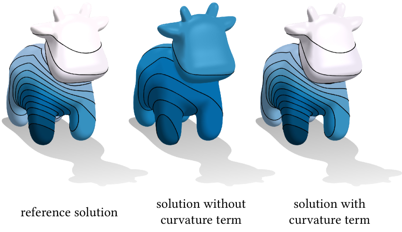
This is, in the case of a planar surface (for which it holds ), exactly the term from our earlier calculation with the planar Hessian energy from (13). Here we also see why minimizers of the naive Hessian energy do not solve the biharmonic equation on curved surfaces: the energy lacks the curvature correction term involving (see Figure 3).
The result from (21) motivates the definition of the following curved Hessian energy:
| (22) |
Minimizers of the energy solve the biharmonic equation on a surface in , unlike minimizers of .
It remains to check what the natural boundary conditions of are. We can find them by checking which biharmonic functions fulfill the boundary terms
We use the same strategy as Stein et al. (2018, Section 4.3): testing with specific subsets of all valid test functions. These subsets are purpose-built to expose the natural boundary conditions of the energy. First, we test with all functions that vanish on the boundary, and thus only have nonzero differential in the normal direction ( for some smooth ). It follows that
| (23) |
i.e., the (curved) Hessian of the solution is linear across the boundary; the second derivative of the function across the boundary is zero. This mirrors the “as-linear-as-possible” condition of Stein et al. (2018, (17)).
Using the same strategy of testing the expression with a specific subset of functions to expose boundary behavior, if we plug in all functions that have zero differential in the normal direction at the boundary (), we get
| (24) |
where is the natural projection of one-forms on the surface to one forms on the boundary, and the subscript on the codifferential implies that this is the codifferential of the boundary manifold in the index . This mirrors the condition from Stein et al. (2018, (18)). In fact, the two natural boundary conditions (23) and (24) of the Hessian energy are exactly the ones of the planar Hessian energy if the domain is a planar surface.
The Hessian energy natural boundary conditions
Like the natural boundary conditions of from Stein et al. (2018, Section 4.3), the natural boundary conditions (23) and (24) of the Hessian energy guarantee that its minimizers
-
•
continue linearly across the boundary in the normal direction (), and
-
•
have limited variation along the boundary (),
as discussed by Stein et al. (2018, Section 4.3). Both boundary conditions are fulfilled by minimizers of in the absence of explicitly enforced boundary conditions.
On planar surfaces, these boundary conditions mean that the null space of the energy contains all linear functions, in contrast to the Laplacian energy with zero Neumann boundary conditions , whose null space only contains constant functions. On closed surfaces, the null space of and is the same: all constant functions.
The natural boundary conditions of the Hessian energy have a physical interpretation. Consider a deforming flat thin plate where displacement is modeled by the function . The plate is not clamped or supported at the boundary in any way: it is a free plate. Then the conditions (24) are the boundary conditions fulfilled by (Courant and Hilbert, 1924, pp. 206-207). These boundary conditions go back at least as far as Rayleigh (1894, p. 355).
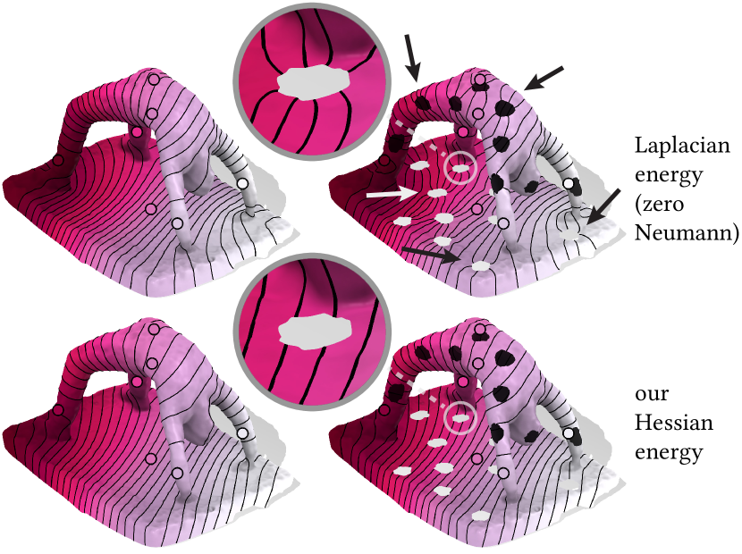
Its natural boundary conditions make the Hessian energy a good choice for ignoring the boundary as much as possible, while maintaining biharmonic behavior everywhere away from the boundary (see Figure 4 where they are contrasted with zero Neumann boundary conditions).
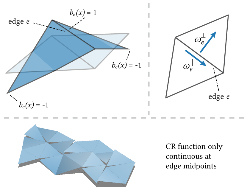
The parallel and perpendicular one-forms for the edge , represented by their dual vectors (top right).
Crouzeix-Raviart functions and their sums are, in general, discontinuous. Continuity is only guaranteed at edge midpoints (bottom).
6. Discretization
We offer a discretization for the curved Hessian energy derived in Section 5. The approach presented here is a simple method using only linear finite elements, intended to make the Hessian energy easily accessible. There are, however, other conceivable ways to discretize this energy, such as, for example, higher-order conforming finite elements (Braess, 2007, II.5).
6.1. Computing the Hessian energy
Discretizing the Hessian energy (22) as written would require us to discretize functions that can be differentiated twice. To avoid this complication we use the mixed finite element method (Boffi et al., 2013) by introducing an intermediate variable and formulate the problem of minimizing as
| (25) |
Using Lagrange multipliers to enforce the constraint , we can write the optimization problem as the saddle problem (where our goal is finding a stationary point)
| (26) |
We discretize the space of scalar functions (containing ) using standard continuous, piecewise linear functions which are a very commonly used finite element. Definitions are found, for example, in Braess (2007, II.5). The basis of this discrete space consists of the , sometimes called “hat functions” (see inset).
![[Uncaptioned image]](/html/1905.09777/assets/x6.png)
We write , and we have the vector .
The space of one-forms (containing ) is discretized using Crouzeix-Raviart one-forms (CROFs), which are described in Section 6.2. The basis of this discrete space are the functions . We write , and we have the vector .
Using these discretizations we can construct the one-form Dirichlet matrix
the differential matrix
the mass matrix
and the curvature matrix
The matrix entries are provided in Appendix A.
Using these matrices, we write the discrete version of (26) as seeking a critical point of the expression
for , . Differentiating with respect to gives . As is invertible, we get the system
| (27) |
This optimization problem can now be solved with a variety of constraints, or mixed with other energy terms, depending on the application.
6.2. Crouzeix-Raviart One-Forms
While there are multiple approaches to discretizing tangent one-forms for triangle meshes, we choose to base our approach on Crouzeix-Raviart finite elements (see Section 2 for a discussion). The advantage of this approach is its simplicity. Crouzeix-Raviart basis functions are only ever nonzero on two adjacent triangles, so every basis function lives on an intrinsically flat domain: the two triangles can be unfolded without distortion. This means that our discretization will account for curvature correctly in the end, without having to explicitly address issues like parallel transport during construction.
6.2.1. Introduction to Crouzeix-Raviart
The scalar Crouzeix-Raviart basis function for the edge is defined to be on the edge itself, on the two vertices opposite the edge, and linear on the two triangles (Braess, 2007, p. 109). For boundary edges, only one triangle needs to be considered. As a result, it is on the midpoints of the edges (see Figure 5, left). The scalar Crouzeix-Raviart element is not continuous, except at the midpoints of edges. This makes it a non-conforming element, and if it is used in a Galerkin method, one speaks of the discontinuous Galerkin method. Despite being nonconforming, it is known to converge for certain problems, most notably the Poisson equation in . (Braess, 2007, III, Theorem 1.5).
6.2.2. One-Forms
The scalar Crouzeix-Raviart element can be used to define a finite element space for one-forms. At the midpoint of every edge of a flat triangle pair, the space of one-forms is spanned by the two forms , such that
| (28) |
where is the (oriented) perpendicular vector of the edge in each triangle, is the (oriented) tangent of the edge , and the angle bracket denotes the pairing of a form with a vector. See Figure 5 (right) for an illustration. The definition of depends on which triangle one is in, but only in an extrinsic way: in the intrinsic geometry of the triangle pair, the edge is completely flat, thus the two covectors defined in each triangle are the same covector intrinsically. Because of this, both and can be easily extended to the triangles adjacent to : since the triangle pair (or the one triangle) is intrinsically flat, parallel transport along the triangles is trivial, and we can easily extend the definition of and to the interior of the triangles adjacent to .
If is the Crouzeix-Raviart basis function for the edge , then we define its two CROF basis function as
| (29) |
Defined this way, CROFs have the correct notion of parallel transport, without having to explicitly account for it. Consider a path through all edge midpoints of edges emanating from a vertex in a counterclockwise direction (see inset). We start with a single tangent vector on the midpoint of one edge, corresponding to a combination of two basis functions, and see what angle we pick up when going around the vertex using our basis functions.
![[Uncaptioned image]](/html/1905.09777/assets/x9.png)
We now go along the path , moving from edge to edge by choosing successive basis functions so that the sum of the basis functions from two adjacent edges is constant on the shared triangle. Doing that corresponds exactly to parallel transport on a cone manifold: the tangential part of the vector at each edge does not change extrinsically at all when crossing the edge along . The perpendicular basis function jumps extrinsically: the angle between normal vectors on each side of the edge is minus the dihedral angle of the edge. At the end of our journey along , when we are back at our original edge, our starting vector picked up angle defect corresponding to the discrete curvature of the mesh. The CROF basis functions have accounted for the discrete curvature of the mesh in the sense of curvature on cone manifolds (Wardetzky, 2006) without having to explicitly account for parallel transport during the construction of the basis functions.
Since every basis function is only supported on at most two triangles, the matrices will be sparse. The matrix is diagonal, which makes it easy to invert. The matrix entries can be found in Appendix A.
6.2.3. The curvature term
Special care needs to be applied when computing the matrix . The Gaussian curvature of an intrinsically flat pair of triangles would appear, at first, to be . But actually, the Gaussian curvature of a polyhedron is entirely concentrated on its vertices (and is zero anywhere else). The integrated Gaussian curvature at a vertex is also known as the angle defect
| (30) |
where the sum is over all faces in the set of faces containing the vertex , and is the angle at vertex in face (Grinspun et al., 2006). The idea of angle defects is very old: it goes back all the way to at least Descartes c. 1630, who showed that the sum of all angle defects of a polyhedron with spherical topology is (Federico, 1982).
We thus interpret the Gaussian curvature of the polyhedron as a collection of delta functions at every vertex, i.e.
| (31) |
where is the Dirac delta. This means that the integral of , where is the Gaussian curvature and is any continuous function over the triangle with vertices , can be written as:
| (32) |
If the function itself is only continuous in each triangle, then we need to distribute the contribution of each triangle accordingly. Let for each vertex and each face in the neighborhood of be coefficients that average the contribution of each face at a vertex, i.e., the sum of the over all faces in the neighborhood of is one. Then
where is the function in the triangle and is the set of all faces in the neighborhood of . We choose to average by tip angle, which corresponds to an integral along a small circle around the vertex. We did not explore other reasonable choices, such as averaging by face area. This formula is used to compute the entries of , they are given in Appendix A.
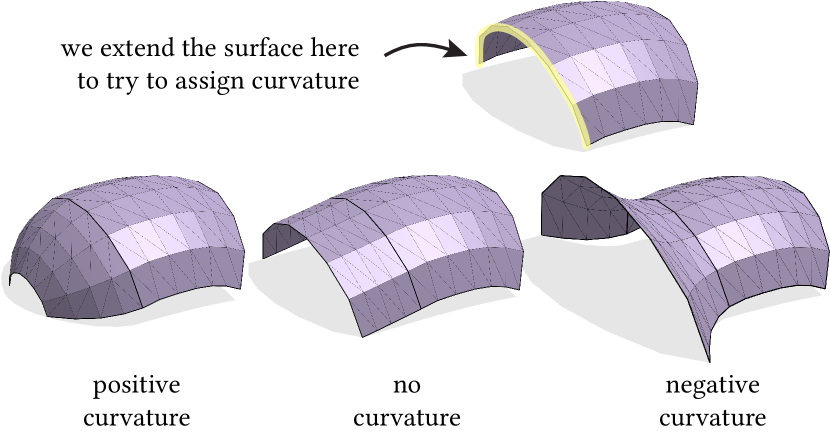
One remaining issue with the angle defect as Gaussian curvature is that the angle defect is not defined at boundary vertices. The problem stems from the fact that the notion of curvature at the boundary of meshes (continuous, piecewise linear surfaces) is not in and of itself meaningful: by choosing to extend the surface in different ways at the boundary we can achieve any arbitrary Gaussian curvature, as can be seen in Figure 6. We choose to set the angle defect to for all boundary vertices, thereby choosing the most developable (intrinsically linear) extension of all possible extensions. This fits in with our as-linear-as-possible boundary conditions, but differs from some conventions of angle defect at the boundary, which define it as the sum of tip angles subtracted from (which is a discretization of geodesic curvature).
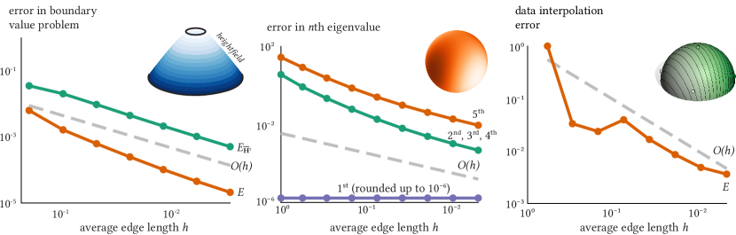
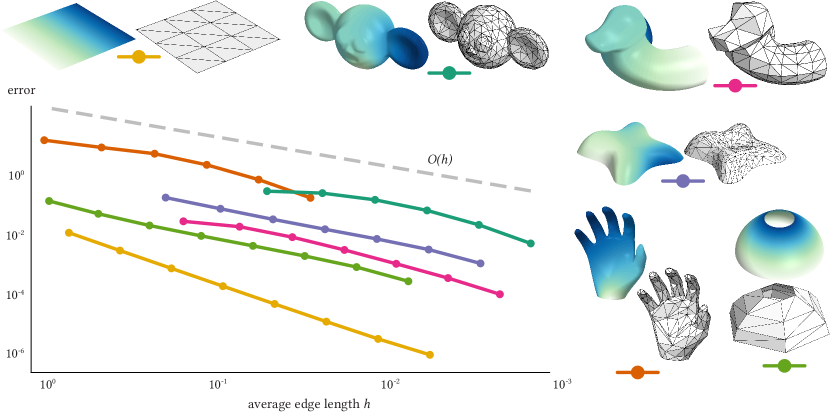
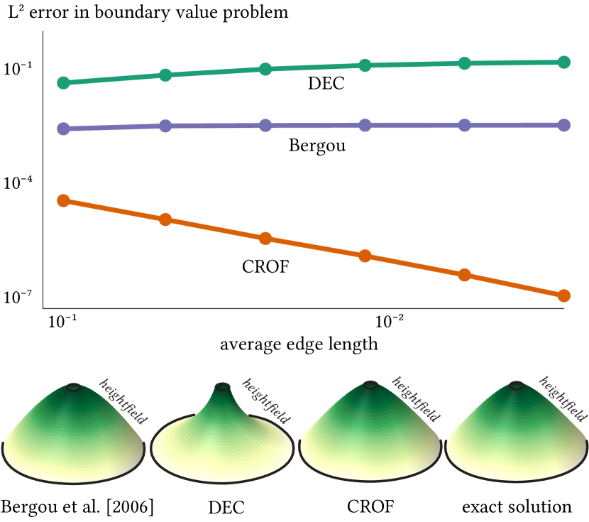
6.3. Observed Numerical Convergence
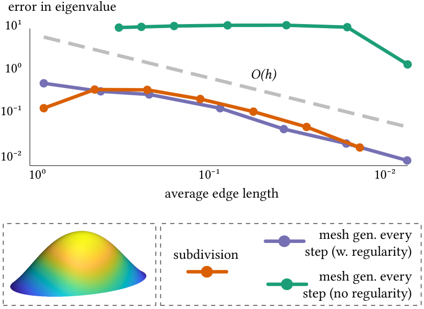
Using our CROF discretization of the Hessian energy to solve a variety of problems, we observe convergence on the order of the average edge length (Figure 9). As can be seen in Figure 8, a successful strategy for obtaining convergence is making sure that the vertices are contained in a smooth surface, and then either refining the mesh through Loop subdivision (Loop, 1987) with a fixed smooth boundary, or generating meshes that fulfill the triangle regularity condition: the ratio of circumcircle to incircle of each triangle (the triangle regularity) is bounded from above and below independent of refinement level. This condition is standard for finite elements (Braess, 2007, Definition 5.1 (uniform triangulation)). The order of convergence and the triangle regularity condition correspond to the discretization of the Laplacian energy with zero Neumann boundary conditions, , with mixed FEM in the flat setting (Scholz, 1978; Jacobson et al., 2010). However, we do not have a proof of convergence for our method to confirm this convergence rate.
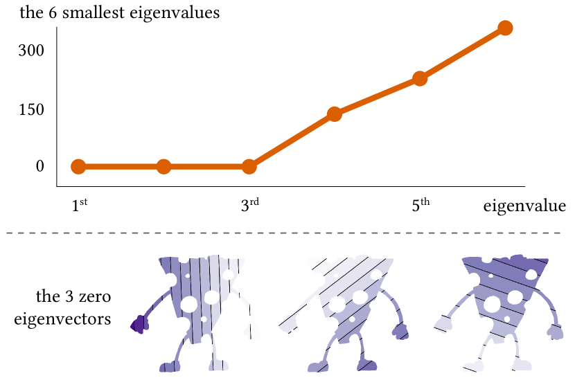
Our method correctly reproduces the first eigenvector of the Laplacian energy on closed surfaces in the experiment proposed by Stein et al. (2018, Section 5.3.1) on a refined mesh (Figure 7). As mentioned in Stein et al. (2018, Section 4.5), discretizations can sometimes exhibit spurious modes in the kernel of the energy, which lead to wrong solutions. We have not proved that this does not happen for our CROF discretization of the Hessian energy, but we have not observed it in our experiments (see Figure 10 for the cheeseman example domain mentioned in Stein et al. (2018, p. 7)).
Further experiments can be found in Appendix B: Figures 15 and 16 feature additional convergence experiments confirming the order of convergence, Figure 17 examines the dependence of the result on the mesh further, and Figure 18 compares our implementation of the Hessian energy with other Hessian energies in the flat case.
7. Applications
We implement the optimization of (27) by constructing a sparse matrix in C++ using Eigen (Guennebaud et al., 2010), and then manipulating and optimizing it in MATLAB (MATLAB, 2019) with mex. For linear equality constraints, we use the optimizer of Jacobson et al. (2019a, min_quad_with_fixed) via the library of Jacobson (2019). Using this approach, complicated constraints are also possible, such as linear and quadratic inequality constraints for more complicated applications. Since the Hessian energy is a quadratic energy, optimizers using the interior point method (such as the solver of Andersen and Andersen (2000)) are appropriate.
7.1. Scattered data interpolation
Like any smoothness energy, the Hessian energy can be used for scattered data interpolation. One solves the following minimization problem, for some given interpolation data
| (33) |
As long as at least three interpolation points are provided, this problem has a solution. This is because the null space of the Hessian energy can have at most all linear functions in it, which is a three-dimensional space, and the null space of the Laplacian energy with zero Neumann boundary conditions contains only constant functions, which is a one-dimensional space (Stein et al., 2018).
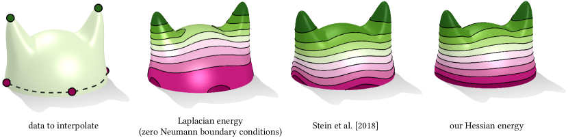
The choice of smoothness energy will greatly influence the quality of the result. The Laplacian energy with zero Neumann boundary conditions, , is a popular method, since it produces smooth, evenly spaced isolines, which results in natural-looking interpolation and extrapolation. This is because the gradient of the solution is relatively uniform across the surface. As can be seen in Figure 11, our curved Hessian energy reproduces the desirable behavior of the Laplacian energy for surfaces without boundary. The implementation of the planar Hessian energy for curved surfaces by Stein et al. (2018) fails to do so: the distance between the isolines varies greatly, for example on the legs. The isolines also experience significant bunching at the rump and back of the horse.
On the other hand, the Laplacian energy is known to produce bias near domain boundaries due to its low-order boundary conditions: isolines of solutions bend so they can be perpendicular to the boundary. This was one of the motivations of Stein et al. (2018), and thus their planar Hessian energy minimizes the influence of the boundary by employing natural boundary conditions that make the function as-linear-as-possible. Figure 4 shows that our Hessian energy does not show the bias at the boundary that the Laplacian energy does: this is because it also has as-linear-as-possible natural boundary conditions.
For this application, our Hessian energy combines the two worlds of Laplacian energy and planar Hessian energy to produce a smoothness energy that is suited for scattered data interpolation on curved surfaces while unbiased by the presence of boundaries (Figure 1, Figure 12). This is helpful if the boundaries of the surface don’t have any physical meaning: perhaps they are the result of a faulty laser scan, or perhaps surface information is simply not available there. The Hessian energy’s natural boundary conditions make a best guess everywhere the data is missing by extrapolating the function linearly across the boundary.
7.2. Data smoothing
Another popular application for smoothness energies is the eponymous data smoothing. This can be used to simply smooth arbitrary data, to denoise noisy data, or to smooth the surface itself via surface fairing. One solves the following Helmholtz-like optimization problem: given an input function to be smoothed,
| (34) |
where the parameter is a trade-off between the input data and the smoothness of the output data.
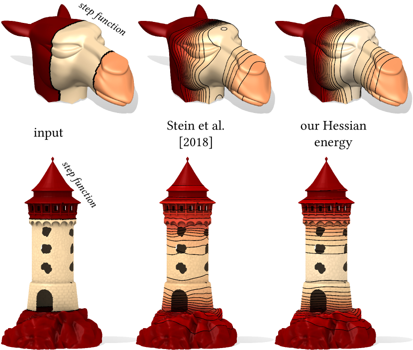
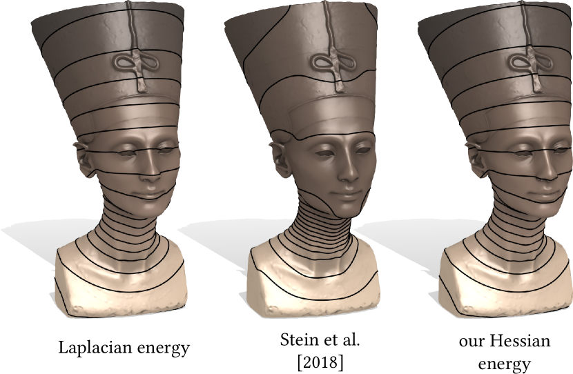
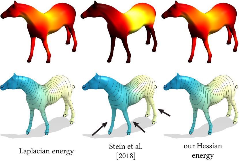
Figure 2 shows our Hessian energy applied to such a smoothing problem. Correctly accounting for curvature by modeling a curved biharmonic equation using the Laplace-Beltrami operator is important here: the figure shows that the approach of Stein et al. (2018) causes distortion in high-curvature regions when smoothing a step function. In this figure the smoothing parameters are chosen to give visually similar amounts of smoothing, which means a slightly larger parameter for the method of Stein et al. (2018).
It is natural to ask why the fact that minimizers of do not solve the biharmonic equation leads to worse results when smoothing the step function of Figure 2, but not for the smoothing problems solved by Stein et al. (2018, Fig. 1, Fig. 11, Fig. 13). These examples all smooth very noisy functions with a lot of variation everywhere on the surface. The step function is the opposite of that: the variation is much more sparse. This allows the error of not accounting for curvature correctly to manifest. In Figure 13 such a denoising problem is solved using the energies (with zero Neumann boundary conditions), (with the implementation of Stein et al. (2018)), and . It can be clearly seen that , the Laplacian energy with zero Neumann boundary conditions, is biased by the boundary, and the isolines near the boundary are distorted so they can be normal to it. The denoised solution using the Hessian energy does not suffer from this, and the isolines ignore the boundary. In regions far away from the boundary it can be observed that the result of denoising with the Hessian energy matches the Laplacian energy with zero Neumann boundary conditions , while the planar Hessian energy differs.
The smoothing problem can also be used to smooth the geometry of the surface itself if the input data from (34) is the vertex positions in each coordinate, and the output data is the new vertex positions. If such a smoothing operation is applied repeatedly, one has a smoothing flow. Figure 14 shows our Hessian energy applied to such a problem. While the method of Stein et al. (2018) can lead to some artifacts due to not accounting for curvature, this does not happen with our curved Hessian energy .
8. Conclusion
In this work we have introduced a smoothing energy for curved surfaces, the Hessian energy. Its minimizers solve the biharmonic equation, and it exhibits the as-linear-as-possible natural boundary conditions in the curved setting that the planar Hessian energy of Stein et al. (2018) exhibits in the flat setting. This Hessian energy can be used in many applications where smoothness energies are required, these smoothness energies should be unbiased by the boundary, and it is crucial that the minimizers of the energy solve the biharmonic equation.
8.1. Limitations
We have no numerical analysis proof for the convergence of our discretization method. We also do not provide any theoretical analysis of the spectrum of our discrete operator. Both are needed to make this discretization reliable, and to improve understanding of the method, where it works, and where it does not.
8.2. Future work
One interesting avenue for future work is to explore alternate discretizations. Higher-order versions of Crouzeix-Raviart basis functions, such as cubic or quintic basis functions, would be an interesting potential improvement. Alternatively, instead of choosing the intermediate variable for the mixed formulation as in (25), a discretization where sounds very promising. This would more closely mirror the mixed formulation of Stein et al. (2018). The CROF approach can be used to define a basis for tensors in the same way as is done for vectors in Section 6.2, based on the parallel and the perpendicular vector at each edge. Using other finite elements to discretize the space of one-forms could also produce new methods. Moreover, future work could explore discretizations of the smooth energy on other surface representations beyond triangle meshes.
A rich source of future work is the numerical analysis of our method. We do not have any proof of convergence, or a solid mathematical analysis of the spectrum of our operator, and while the experiments in Section 6.3 provide some evidence for problems that can be solved with our discretization of , a thorough numerical analysis treatment of our discretization would be valuable to exactly identify the strengths and weaknesses of our method. Our Crouzeix-Raviart discretization is a potential candidate for spurious modes, since the finite element is non-conforming, even though we have not observed them in practice. The method of English and Bridson (2008) is an example of a Crouzeix-Raviart discretization that works for many cases, but where specific triangle configurations exist that lead to spurious modes (Quaglino, 2012, Section 4.4.2). The properties of minimizers of the discrete energies also warrant further investigation: it is unclear which properties of smooth minimizers they actually inherit, and which properties only hold in the limit.
Another interesting direction for future work is to consider additional applications. Smoothness energies have many uses, and if such an application has to be unbiased by the boundary even on heavily curved surfaces, our Hessian energy is a powerful tool. Applications could include animation (Jacobson et al., 2011), distance computation (Crane et al., 2013b), and more.
Moreover, our simple Crouzeix-Raviart discretization of the one-form Dirichlet energy containing covariant derivatives from Section 6.2 offers an interesting approach to discretize the vector Dirichlet energy in a wide variety of applications. Potential applications include vector field design (Knöppel et al., 2013), parallel transport of vectors (Sharp et al., 2018), and many more (Azencot et al., 2015; Liu et al., 2016; Corman and Ovsjanikov, 2019).
The smoothing parameter was chosen to produce a similar amount of smoothing in both methods. Three smoothing steps were computed.
Acknowledgements
We thank the libigl data repository (Jacobson et al., 2019b) (horse, camel, cross lilium, hand, puppet head by Cosmic blobs), the Stanford 3D Scanning Repository (Graphics, 2014) (armadillo), Crane (2018) (rubber duck, man-bridge, spot the cow, Nefertiti by Nora Al-Badri and Jan Nikolai Nelles), Jacobson (2013) (various cartoons in Figure 16), YahooJAPAN (2013) (plane), jansentee3d (2018) (tower), and Javo (2016) (helmet) for some of the meshes used in this work.
This work is funded in part by the National Science Foundation Awards CCF-17-17268 and IIS-17-17178. This research is funded in part by NSERC Discovery (RGPIN2017-05235, RGPAS-2017-507938), the Canada Research Chairs Program, the Fields Centre for Quantitative Analysis and Modelling and gifts by Adobe Systems, Autodesk and MESH Inc. This work is partially supported by the DFG project 282535003: Geometric curvature functionals: energy landscape and discrete methods.
We thank Anne Fleming, Henrique Maia and Peter Chen for proofreading.
References
- (1)
- Andersen and Andersen (2000) E. D. Andersen and K. D. Andersen. 2000. The mosek interior point optimizer for linear programming: an implementation of the homogeneous algorithm. In High Performance Optimization. Kluwer Academic Publishers, 197–232.
- Azencot et al. (2015) Omri Azencot, Maks Ovsjanikov, Frédéric Chazal, and Mirela Ben-Chen. 2015. Discrete Derivatives of Vector Fields on Surfaces – An Operator Approach. ACM Trans. Graph. 34, 3 (May 2015), 29:1–29:13.
- Baran and Popovic (2007) Ilya Baran and Jovan Popovic. 2007. Automatic Rigging and Animation of 3D Characters. ACM Trans. Graph. 26, 3 (July 2007), 72–es.
- Bergou et al. (2006) Miklos Bergou, Max Wardetzky, David Harmon, Denis Zorin, and Eitan Grinspun. 2006. A Quadratic Bending Model for Inextensible Surfaces. In Proceedings of the Fourth Eurographics Symposium on Geometry Processing. Aire-la-Ville, Switzerland, 227–230.
- Bergou et al. (2008) Miklós Bergou, Max Wardetzky, Stephen Robinson, Basile Audoly, and Eitan Grinspun. 2008. Discrete Elastic Rods. ACM Trans. Graph. 27, 3 (Aug. 2008), 63:1–63:12.
- Bochner (1946) S. Bochner. 1946. Vector fields and Ricci curvature. Bull. Amer. Math. Soc. 52, 9 (1946), 776–797.
- Boffi et al. (2013) Daniele Boffi, Franco Brezzi, and Michel Fortin. 2013. Mixed Finite Element Methods and Applications. Springer-Verlag Berlin Heidelberg.
- Botsch and Kobbelt (2004) Mario Botsch and Leif Kobbelt. 2004. An Intuitive Framework for Real-Time Freeform Modeling. ACM Trans. Graph. 23, 3 (Aug. 2004), 630–634.
- Braess (2007) Dietrich Braess. 2007. Finite Elements (3rd ed.). Cambridge University Press.
- Brandt et al. (2018) Christopher Brandt, Leonardo Scandolo, Elmar Eisemann, and Klaus Hildebrandt. 2018. Modeling n-Symmetry Vector Fields Using Higher-Order Energies. ACM Trans. Graph. 37, 2 (March 2018), 18:1–18:18.
- Brenner (2015) Susanne C. Brenner. 2015. Forty Years of the Crouzeix-Raviart element. Numerical Methods for Partial Differential Equations 31, 2 (2015), 367–396.
- Corman and Ovsjanikov (2019) Etienne Corman and Maks Ovsjanikov. 2019. Functional Characterization of Deformation Fields. ACM Trans. Graph. 38, 1 (Jan. 2019), 8:1–8:19.
- Courant and Hilbert (1924) R. Courant and D. Hilbert. 1924. Methoden der Mathematischen Physik – Erster Band. Julius Springer, Berlin.
- Crane (2018) Keenan Crane. 2018. Keenan’s 3D Model Repository. https://www.cs.cmu.edu/ kmcrane/Projects/ModelRepository/.
- Crane et al. (2010) Keenan Crane, Mathieu Desbrun, and Peter Schröder. 2010. Trivial Connections on Discrete Surfaces. Computer Graphics Forum (SGP) 29, 5 (2010), 1525–1533.
- Crane et al. (2013a) Keenan Crane, Ulrich Pinkall, and Peter Schröder. 2013a. Robust Fairing via Conformal Curvature Flow. ACM Trans. Graph. 32, 4, Article Article 61 (July 2013), 10 pages.
- Crane et al. (2013b) Keenan Crane, Clarisse Weischedel, and Max Wardetzky. 2013b. Geodesics in Heat: A New Approach to Computing Distance Based on Heat Flow. ACM Trans. Graph. 32, 5 (Oct. 2013), 152:1–152:11.
- Crouzeix and Raviart (1973) Michel Crouzeix and P.-A. Raviart. 1973. Conforming and nonconforming finite element methods for solving the stationary Stokes equations I. ESAIM: Mathematical Modelling and Numerical Analysis - Modélisation Mathématique et Analyse Numérique 7, R3 (1973), 33–75.
- Desbrun et al. (1999) Mathieu Desbrun, Mark Meyer, Peter Schröder, and Alan H. Barr. 1999. Implicit Fairing of Irregular Meshes Using Diffusion and Curvature Flow. In Proceedings of the 26th Annual Conference on Computer Graphics and Interactive Techniques (SIGGRAPH ’99). ACM Press/Addison-Wesley Publishing Co., New York, NY, USA, 317–324.
- Didas et al. (2009) Stephan Didas, Joachim Weickert, and Bernhard Burgeth. 2009. Properties of Higher Order Nonlinear Diffusion Filtering. Journal of Mathematical Imaging and Vision 35, 3 (2009), 208–226.
- Donoho and Grimes (2003) David L. Donoho and Carrie Grimes. 2003. Hessian eigenmaps: Locally linear embedding techniques for high-dimensional data. Proceedings of the National Academy of Sciences 100, 10 (2003), 5591–5596. https://doi.org/10.1073/pnas.1031596100
- Duffin (1959) R. J. Duffin. 1959. Distributed and Lumped Networks. Journal of Mathematics and Mechanics 8, 5 (1959), 793–826.
- Dziuk (1988) Gerhard Dziuk. 1988. Finite Elements for the Beltrami operator on arbitrary surfaces. Springer Berlin Heidelberg, 142–155.
- English and Bridson (2008) Elliot English and Robert Bridson. 2008. Animating Developable Surfaces Using Nonconforming Elements. ACM Trans. Graph. 27, 3 (Aug. 2008), 66:1–66:5.
- Evans (2010) Lawrence C. Evans. 2010. Partial Differential Equations: (2nd ed.). American Mathematical Society.
- Federico (1982) P. J. Federico. 1982. Descartes on Polyhedra. Springer-Verlag New York Inc.
- Fisher et al. (2007) Matthew Fisher, Peter Schröder, Mathieu Desbrun, and Hugues Hoppe. 2007. Design of Tangent Vector Fields. In ACM SIGGRAPH 2007 Papers (SIGGRAPH ’07). ACM, New York, NY, USA.
- Gazzola et al. (2010) Filippo Gazzola, Hans-Christoph Grunau, and Guido Sweers. 2010. Polyharmonic Boundary Value Problems. Springer-Verlag Berlin Heidelberg.
- Georgiev (2004) Todor Georgiev. 2004. Photoshop Healing Brush: a Tool for Seamless Cloning. Proc. of ECCV (2004).
- Graphics (2014) Stanford Graphics. 2014. The Stanford 3D Scanning Repository. http://graphics.stanford.edu/data/3Dscanrep/.
- Grinspun et al. (2006) Eitan Grinspun, Mathieu Desbrun, Konrad Polthier, Peter Schröder, and Ari Stern. 2006. Discrete Differential Geometry: An Applied Introduction. In ACM SIGGRAPH 2006 Courses (SIGGRAPH ’06). ACM, New York, NY, USA.
- Guennebaud et al. (2010) Gaël Guennebaud, Benoît Jacob, et al. 2010. Eigen v3. http://eigen.tuxfamily.org.
- Hildebrandt et al. (2006) Klaus Hildebrandt, Konrad Polthier, and Max Wardetzky. 2006. On the convergence of metric and geometric properties of polyhedral surfaces. Geometriae Dedicata 123, 1 (December 2006), 89–112.
- Jacobson (2013) Alec Jacobson. 2013. Algorithms and Interfaces for Real-Time Deformation of 2D and 3D Shapes. Ph.D. Dissertation. ETH Zürich.
- Jacobson (2019) Alec Jacobson. 2019. gptoolbox – Geometry Processing Toolbox. https://github.com/alecjacobson/gptoolbox.
- Jacobson et al. (2011) Alec Jacobson, Ilya Baran, Jovan Popović, and Olga Sorkine. 2011. Bounded Biharmonic Weights for Real-time Deformation. ACM Trans. Graph. 30, 4 (July 2011), 78:1–78:8.
- Jacobson et al. (2019a) Alec Jacobson, Daniele Panozzo, et al. 2019a. libigl: A simple C++ geometry processing library. http://libigl.github.io/libigl/.
- Jacobson et al. (2019b) Alec Jacobson, Daniele Panozzo, et al. 2019b. libigl tutorial data. https://github.com/libigl/libigl-tutorial-data.
- Jacobson et al. (2010) Alec Jacobson, Elif Tosun, Olga Sorkine, and Denis Zorin. 2010. Mixed Finite Elements for Variational Surface Modeling. Computer Graphics Forum 29, 5 (2010), 1565–1574.
- Jacobson et al. (2012) Alec Jacobson, Tino Weinkauf, and Olga Sorkine. 2012. Smooth Shape-Aware Functions with Controlled Extrema. Comput. Graph. Forum 31, 5 (Aug. 2012), 1577–1586.
- jansentee3d (2018) jansentee3d. 2018. Dragon Tower. https://www.thingiverse.com/thing:3155868.
- Javo (2016) Javo. 2016. Big Gladiator Helmet. https://www.thingiverse.com/thing:1345281.
- Joshi et al. (2007) Pushkar Joshi, Mark Meyer, Tony DeRose, Brian Green, and Tom Sanocki. 2007. Harmonic Coordinates for Character Articulation. ACM Trans. Graph. 26, 3 (July 2007), 71–es.
- Jost (2011) Jürgen Jost. 2011. Riemannian Geometry and Geometric Analysis. Springer-Verlag Berlin Heidelberg.
- Kim et al. (2009) Kwang I. Kim, Florian Steinke, and Matthias Hein. 2009. Semi-supervised Regression using Hessian energy with an application to semi-supervised dimensionality reduction. In Advances in Neural Information Processing Systems 22, Y. Bengio, D. Schuurmans, J. D. Lafferty, C. K. I. Williams, and A. Culotta (Eds.). Curran Associates, Inc., 979–987.
- Knöppel et al. (2013) Felix Knöppel, Keenan Crane, Ulrich Pinkall, and Peter Schröder. 2013. Globally Optimal Direction Fields. ACM Trans. Graph. 32, 4 (July 2013), 59:1–59:10.
- Knöppel et al. (2015) Felix Knöppel, Keenan Crane, Ulrich Pinkall, and Peter Schröder. 2015. Stripe Patterns on Surfaces. ACM Trans. Graph. 34, 4 (July 2015), 39:1–39:11.
- Lee (1997) John M. Lee. 1997. Riemannian Manifolds. Springer-Verlag New York, Inc.
- Lefkimmiatis et al. (2011) Stamatis Lefkimmiatis, Aurélien Bourquard, and Michael Unser. 2011. Hessian-Based Norm Regularization for Image Restoration With Biomedical Applications. IEEE transactions on image processing : a publication of the IEEE Signal Processing Society 21 (09 2011), 983–95.
- Levin et al. (2004) Anat Levin, Dani Lischinski, and Yair Weiss. 2004. Colorization Using Optimization. In ACM SIGGRAPH 2004 Papers (SIGGRAPH ’04). Association for Computing Machinery, New York, NY, USA, 689–694.
- Lipman et al. (2010) Yaron Lipman, Raif M. Rustamov, and Thomas A. Funkhouser. 2010. Biharmonic Distance. ACM Trans. Graph. 29, 3 (July 2010), 27:1–27:11.
- Liu et al. (2016) Beibei Liu, Yiying Tong, Fernando De Goes, and Mathieu Desbrun. 2016. Discrete Connection and Covariant Derivative for Vector Field Analysis and Design. ACM Trans. Graph. 35, 3 (March 2016), 23:1–23:17.
- Liu et al. (2015) X. Y. Liu, C. H. Lai, and K. A. Pericleous. 2015. A Fourth-Order Partial Differential Equation Denoising Model with an Adaptive Relaxation Method. Int. J. Comput. Math. 92, 3 (March 2015), 608–622.
- Loop (1987) Charles Loop. 1987. Smooth Subdivision Surfaces Based on Triangles. Master’s thesis. University of Utah.
- Lysaker et al. (2003) M. Lysaker, A. Lundervold, and Xue-Cheng Tai. 2003. Noise removal using fourth-order partial differential equation with applications to medical magnetic resonance images in space and time. IEEE Transactions on Image Processing 12, 12 (Dec 2003), 1579–1590.
- MacNeal (1949) Richard H. MacNeal. 1949. The solution of partial differential equations by means of electrical networks. Ph.D. Dissertation. California Institute of Technology.
- MATLAB (2019) MATLAB. 2019. version 9.6 (R2019a). The MathWorks Inc.
- Nocedal and Wright (2006) Jorge Nocedal and Stephen J. Wright. 2006. Numerical Optimization (2nd ed.). Springer Science + Business Media, LLC.
- Peter et al. (2016) Pascal Peter, Sebastian Hoffmann, Frank Nedwed, Laurent Hoeltgen, and Joachim Weickert. 2016. Evaluating the True Potential of Diffusion-Based Inpainting in a Compression Context. Image Commun. 46, C (Aug. 2016), 40–53.
- Petersen (2006) Peter Petersen. 2006. Riemannian Geometry (second ed.). Springer Science + Business Media, LLC.
- Polthier and Schmies (1998) Konrad Polthier and Markus Schmies. 1998. Straightest Geodesics on Polyhedral Surfaces. Springer Berlin Heidelberg, 135–150. https://doi.org/10.1007/978-3-662-03567-2_11
- Quaglino (2012) Alessio Quaglino. 2012. Membrane locking in discrete shell theories. Ph.D. Dissertation. Universität Göttingen.
- Ray et al. (2009) Nicolas Ray, Bruno Vallet, Laurent Alonso, and Bruno Levy. 2009. Geometry-aware Direction Field Processing. ACM Trans. Graph. 29, 1 (Dec. 2009), 1:1–1:11.
- Rayleigh (1894) John William Strutt Rayleigh. 1894. The Theory of Sound. Vol. 1st. Macmillan and Co.
- Scholz (1978) Reinhard Scholz. 1978. A mixed method for 4th order problems using linear finite elements. RAIRO. Analyse numérique 12, 1 (1978), 85–90.
- Sharp et al. (2018) Nicholas Sharp, Yousuf Soliman, and Keenan Crane. 2018. The Vector Heat Method. CoRR abs/1805.09170 (2018). arXiv:1805.09170 http://arxiv.org/abs/1805.09170
- Sorkine et al. (2004) O. Sorkine, D. Cohen-Or, Y. Lipman, M. Alexa, C. Rössl, and H.-P. Seidel. 2004. Laplacian Surface Editing. In Proceedings of the 2004 Eurographics/ACM SIGGRAPH Symposium on Geometry Processing. ACM, New York, NY, USA, 175–184.
- Stein et al. (2018) Oded Stein, Eitan Grinspun, Max Wardetzky, and Alec Jacobson. 2018. Natural Boundary Conditions for Smoothing in Geometry Processing. ACM Trans. Graph. 37, 2 (May 2018), 23:1–23:13.
- Sýkora et al. (2014) Daniel Sýkora, Ladislav Kavan, Martin Čadík, Ondřej Jamriška, Alec Jacobson, Brian Whited, Maryann Simmons, and Olga Sorkine-Hornung. 2014. Ink-and-Ray: Bas-Relief Meshes for Adding Global Illumination Effects to Hand-Drawn Characters. ACM Trans. Graph. 33, 2, Article Article 16 (April 2014), 15 pages.
- Vaxman et al. (2016) Amir Vaxman, Marcel Campen, Olga Diamanti, Daniele Panozzo, David Bommes, Klaus Hildebrandt, and Mirela Ben-Chen. 2016. Directional Field Synthesis, Design, and Processing. Computer Graphics Forum (2016).
- Wang et al. (2015) Yu Wang, Alec Jacobson, Jernej Barbič, and Ladislav Kavan. 2015. Linear subspace design for real-time shape deformation. ACM Trans. Graph. (TOG) 34, 4 (2015), 57:1–57:11.
- Wang et al. (2017) Yu Wang, Alec Jacobson, Jernej Barbič, and Ladislav Kavan. 2017. Error in “Linear Subspace Design for Real-Time Shape Deformation”. Tech. Report.
- Wardetzky (2006) Max Wardetzky. 2006. Discrete Differential Operators on Polyhedral Surfaces – Convergence and Approximation. Ph.D. Dissertation. FU Berlin.
- Wardetzky et al. (2007) Max Wardetzky, Saurabh Mathur, Felix Kälberer, and Eitan Grinspun. 2007. Discrete Laplace Operators: No Free Lunch. In Proceedings of the Fifth Eurographics Symposium on Geometry Processing (SGP ’07). Eurographics Association, Goslar, DEU, 33–37.
- Weber et al. (2012) Ofir Weber, Roi Poranne, and Craig Gotsman. 2012. Biharmonic Coordinates. Computer Graphics Forum 31, 8 (2012), 2409–2422.
- Weber et al. (2007) Ofir Weber, Olga Sorkine, Yaron Lipman, and Craig Gotsman. 2007. Context-Aware Skeletal Shape Deformation. Computer Graphics Forum 26, 3 (2007), 265–274.
- Weinkauf et al. (2010) Tino Weinkauf, Yotam Gingold, and Olga Sorkine. 2010. Topology-based Smoothing of 2D Scalar Fields with C1-Continuity. Computer Graphics Forum 29, 3 (2010).
- Weisstein (2019) Eric W. Weisstein. 2019. Monge Patch. From MathWorld–A Wolfram Web Resource. http://mathworld.wolfram.com/MongePatch.html
- Weitzenböck (1885) Roland Weitzenböck. 1885. Invariantentheorie. P. Noordhoff.
- YahooJAPAN (2013) YahooJAPAN. 2013. Plane. https://www.thingiverse.com/thing:182252.
Appendix
Appendix A Implementation
The entries for each of the matrices defined in Section 6.1 needed to construct the system matrices used in (27) are as follows. Let be an oriented edge from the vertex to . The two triangles adjacent to are and , and is an oriented edge from the vertex to . The entries of the symmetric CROF vector Dirichlet matrix on the triangle are
| (35) |
where is the double area of the triangle , is the angle in the triangle at the vertex , and is the length of the edge from vertex to . If one of the edges has reversed orientation in the triangle with respect to its global orientation, its off-diagonal entries get multiplied by . These are only the terms for the triangle . One must add the terms for all triangles and all pairs of edges in that triangle to compute the full matrix . We suggest looping through all triangles, and adding the terms for each triangle to the respective entries of the matrix corresponding to the edges. This can easily be parallelized with a parallel_for loop.
The entries of the diagonal CROF mass matrix on the triangle are
| (36) |
The entries of the differential matrix on the triangle for each edge are
| (37) |
where is the vertex at the tail of the edge , and is at its tip. If one of the edges has reversed orientation in the triangle with respect to its global orientation, its entries get multiplied by .
The entries of the curvature correction matrix on the triangle are
| (38) |
where is the angle defect at the vertex and is the angle sum at the vertex . If one of the edges has reversed orientation in the triangle with respect to its global orientation, its off-diagonal entries get multiplied by .
Appendix B Additional experiments
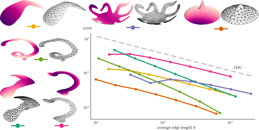
Figure 15 features a series of convergence experiments that shows the convergence of a boundary value problem on a variety of meshes to the highest-resolution solutions. In Figure 16, a series of forward problems is solved, where the Hessian energy of a function is measured on a curved surface, and because both the function and the surface embedding are known, the exact solution is also known. This is used to measure the error. In both these examples, convergence of the order of the average edge length is observed.
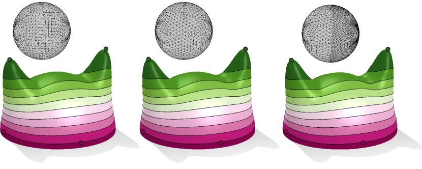
Figure 17 shows that for different meshings of the same surface, very similar results are achieved, and the method is thus robust to remeshing. In Figure 18 our CROF implementation of the Hessian energy is compared with various Hessian energies discussed by Stein et al. (2018) in the flat annulus setting, where the exact solution is known.