Workflow Design Analysis for High Resolution Satellite Image Analysis

Abstract

Ecological sciences are using imagery from a variety of sources to monitor and survey populations and ecosystems. Very High Resolution (VHR) satellite imagery provide an effective dataset for large scale surveys. Convolutional Neural Networks have successfully been employed to analyze such imagery and detect large animals. As the datasets increase in volume, O(TB), and number of images, O(1k), utilizing High Performance Computing (HPC) resources becomes necessary. In this paper, we investigate a task-parallel data-driven workflows design to support imagery analysis pipelines with heterogeneous tasks on HPC. We analyze the capabilities of each design when processing a dataset of 3,000 VHR satellite images for a total of 4 TB. We experimentally model the execution time of the tasks of the image processing pipeline. We perform experiments to characterize the resource utilization, total time to completion, and overheads of each design. Based on the model, overhead and utilization analysis, we show which design approach to is best suited in scientific pipelines with similar characteristics.

I Introduction

A growing number of scientific domains are adopting workflows that use multiple analysis algorithms to process a large number of images. The volume and scale of data processing justifies the use of parallelism, tailored programming models and high performance computing (HPC) resources. While these features create a large design space, the lack of architectural and performance analyses makes it difficult to chose among functionally equivalent implementations.

In this paper we focus on the design of computing frameworks that support the execution of heterogeneous tasks on HPC resources to process large imagery datasets. These tasks may require one or more CPUs and GPUs, implement diverse functionalities and execute for different amounts of time. Typically, tasks have data dependences and are therefore organized into workflows. Due to task heterogeneity, executing workflows poses the challenges of effective scheduling, correct resource binding and efficient data management. HPC infrastructures exacerbate these challenges by privileging the execution of single, long-running jobs.

From a design perspective, a promising approach to address these challenges is isolating tasks from execution management. Tasks are assumed to be self-contained programs which are executed in the operating system (OS) environment of HPC compute nodes. Programs implement the domain-specific functionalities required by use cases while computing frameworks implement resource acquisition, task scheduling, resource binding, and data management.

Compared to approaches in which tasks are functions or methods, a program-based approach offers several benefits as, for example, simplified implementation of execution management, support of general purpose programming models, and separate programming of management and domain-specific functionalities. Nonetheless, program-based designs also impose performance limitations, including OS-mediated intertask communication and task spawning overheads, as programs execute as OS processes and do not share a memory space.

Due to their performance limitations, program-based designs of computing frameworks are best suited to execute compute-intense workflows in which each task requires a certain amount of parallelism and runs from several minutes to hours. The emergence of workflows that require heterogeneous, compute-intense tasks to process large amount of data is pushing the boundaries of program-based designs, especially when scale requirements suggest the use of modern HPC infrastructures with large number of CPUs/GPUs and dedicated data facilities.

We use a paradigmatic use case from the polar science domain to evaluate three alternative program-based designs, and experimentally characterize and compare their performance. Our use case requires us to analyze satellite images of Antarctica to detect pack-ice seals taken across a whole calendar year. The resulting dataset consists of $3,097$ images for a total of $\approx 4$ TB. The use case requires us to repeatedly process these images, running both CPUs and GPUs code that exchange several GB of data. The first design uses a pipeline to independently process each image, while the second and third designs use the same pipeline to process a series of images with differences in how images are bound to available compute nodes.

This paper offers three main contributions: (1) a precise indication of how to further the implementation of our workflow engine so to support the class of use cases we considered while minimizing workflow time to completion and maximizing resource utilization; (2) specific design guidelines for supporting data-driven, compute-intense workflows on high-performance computing resources with a task-based computing framework; and (3) an experiment-based methodology to compare design performance of alternative designs that does not depend on the considered use case and computing framework.

The paper is organized as follows. §III presents the use case in more detail and discuses its computational requirements as well as the individual stages of the pipeline. §II provides a survey of the state of the art and §IV discusses the three designs in detail. §V presents our performance evaluation, discussing the results of our experiments and §VI concludes the paper.

II Related Work

Several tools and frameworks are available for image analysis based on diverse designs and programming paradigms, and implemented for specific resources. Numerous image analytics frameworks for medical, astronomical, and other domain specific imagery provide MapReduce implementations. MaReIA [1], built for medical image analysis, is based on Hadoop and Spark [2]. Kira [3], built for astronomical image analysis, is also built on top of Spark and pySpark, allowing users to define custom analysis applications. Further, Ref. [4] proposes a Hadoop-based cloud Platform as a Service, utilizing Hadoop’s streaming capabilities to reduce filesystem reads and writes. These frameworks support clouds and/or commodity clusters for execution.

BIGS [5] is a framework for image processing and analysis. BIGS is based on the master-worker model and supports heterogeneous resources, such as clouds, grids and clusters. BIGS deploys a number of workers to resources, which query its scheduler for jobs. When a worker can satisfy the data dependencies of a job it becomes responsible to execute it. BIGS workers can be deployed on any type of supported resource. The user is responsible to define the input, processing pipeline, and launch BIGS workers. As soon as a worker is available execution starts. In addition, BISGS offers a diverse set of APIs for developers. BIGS approach is very close to Design 1 we described in §IV-A.

LandLab [6] is a framework for building, coupling and exploring two-dimensional numerical models for Earth-surface dynamics. LandLab provides a library of processing constructs. Each construct is a numerical representation of a geological process. Multiple components are used together allowing the simulation of multiple processes acting on a grid. The design of each component is intended to work in a plug-and-play fashion. Components couple simply and quickly. Parallelizing Landlab components is left to the developer.

Image analysis libraries, frameworks and applications have been proposed for HPC resources. PIMA(GE)² Library [7] provides a low-level API for parallel image processing using MPI and CUDA. SIBIA [8] is a framework for coupling biophysical models with medical image analysis, and provides parallel computational kernels through MPI and vectorization. Ref. [9] proposes a scalable medical image analysis service. This service uses DAX [10] as an engine to create and execute image analysis pipelines. Tomosaic [11] is a Python framework, used for medical imaging, employing MPI4py to parallelize different parts of the workflow.

Petruzza et al. [12] describe a scalable image analysis library. Their approach defines pipelines as data-flow graphs, with user defined functions as tasks. Charm++ is used as the workflow management layer, by abstracting the execution level details, allowing execution on local workstations and HPC resources. Teodoro et al. [13] define a master-worker framework supporting image analysis pipelines on heterogeneous resources. The user defines an abstract dataflow and the framework is responsible to schedule tasks on CPU or GPUs. Data communication and coordination is done via MPI. Ref. [14] proposes the use of the UNICORE [15] to define image analysis workflows on HPCs.

Our approach proposes designs for image analysis pipelines that are domain independent. In addition, the workflow and runtime systems we use allow execution on multiple HPC resources with no change in our approach. Furthermore, parallelization is inferred in one of the proposed designs, allowing correct execution regardless of the multi-core or multi-GPU capabilities of the used resource.

All the above, except Ref. [3], focus on characterizing the performance of the proposed solution. Ref. [3] compares different implementations, one with Spark, one with pySpark, and an MPI C-based implementation. This comparison is based on the weak and strong scaling properties of the approaches. Our approach offers a well-defined methodology to compare different designs for task-based and data-driven pipelines with heterogeneous tasks.

III Satellite Imagery Analysis Application

Imagery employed by ecologists as a tool to survey populations and ecosystems come from a wide range of sensors, e.g., camera-trap surveys [16] and aerial imagery transects [17]. However, most traditional methods can be prohibitively labor-intensive when employed at large scales or in remote regions. Very High Resolution (VHR) satellite imagery provides an effective alternative to perform large scale surveys at locations with poor accessibility such as surveying Antarctic fauna [18]. To take full advantage from increasingly large VHR imagery, and reach the spatial and temporal breadths required to answer ecological questions, it is paramount to automate image processing and labeling.

Convolutional Neural Networks (CNN) represent the state-of-the-art for nearly every computer vision routine. For instance, ecologists have successfully employed CNNs to detect large mammals in airborne imagery [19, 20], and camera-trap survey imagery [21]. We use a Convolutional Neural Network (CNN) to survey Antarctic pack-ice seals in VHR imagery. Pack-ice seals are a main component of the Antarctic food web [22]: estimating the size and trends of their populations is key to understanding how the Southern Ocean ecosystem copes with climate change [23] and fisheries [24].

For this use case, we process WorldView 3 (WV03) panchromatic imagery as provided by DigitalGlobe Inc. This dataset has the highest available resolution for commercial satellite imagery. We refrain from using imagery from other sensors because pack-ice seals are not clearly visible at lower resolutions. For our CNN architecture, we use a U-Net [25] variant that counts seals with an added regression branch and locates them using a seal intensity heat map. To train our CNN, we use a training set with $88k$ hand-labeled images, cropped from WV03 imagery, where every image has a correspondent seal count and a class label (i.e., seal vs. non-seal). For hyper-parameter search, we train CNN variants for 75 epochs (i.e., 75 complete runs through the training set) using an Adam optimizer [26] with a learning rate of $10^{-3}$ and tested against a validation set.

We use the best performing model on an archive of over $3,097$ WV03 images, with a total dataset size of $\approx 4$ TB. Due to limitations on GPU memory, it is necessary to tile WV03 images into smaller patches before sending input imagery through the seal detection CNN. Taking tiled imagery as input, the CNN outputs the latitude and longitude of each detected seal. While the raw model output still requires statistical treatment, such ‘mock-run’ emulates the scale necessary to perform a comprehensive pack-ice seal census. We order the tiling and seal detection stages into a pipeline that can be re-run whenever new imagery is obtained. This allows domain scientists to create seal abundance time series that can aid in Southern Ocean monitoring.

IV Workflow Design and Implementation

Computationally, the use case described in §III presents three main challenges: heterogeneity, scale and repeatability. The images of the use case dataset vary in size with a wide distribution. Each image requires tiling, per tile counting of seal populations and result aggregation across tiles. Tiling is memory intensive while counting is computationally intensive, requiring CPU and GPU implementations, respectively. Whenever the image dataset is updated, it needs to be reprocessed.

We address these challenges by codifying image analysis into a workflow. We then execute this workflow on HPC resources, leveraging the concurrency, storage systems and compute speed they offer to reduce time to completion. Typically, this type of workflow consists of a sequence (i.e., pipeline) of tasks, each performing part of the end-to-end analysis on one or more images. The implementation of this workflow varies, depending on the API of the chosen workflow system and its supported runtime system. Here, we compare two common designs: one in which each image is processed independently by a dedicated pipeline; the other in which a pipeline processes multiple images.

Note that both designs separate the functionalities required to process each image from the functionalities used to coordinate the processing of multiple images. This is consistent with moving away from vertical, end-to-end single-point solutions, favoring designs and implementations that satisfy multiple use cases, possibly across diverse domains. Accordingly, the two designs we consider, implement, and characterize use two tasks (i.e., programs) to implement the tiling and counting functionalities required by the use case.

Both designs are functionally equivalent, in that they both enable the analysis of the given image dataset. Nonetheless, each design leads to different amounts of concurrency, resource utilization and overheads, depending on data/compute affinity, scheduling algorithm, and coordination between CPU and GPU computations. Based on a performance analysis, it will be possible to know which design entails the best tradeoffs for common metrics as total execution time or resource utilization.

Consistent with HPC resources currently available for research and our use case, we make three architectural assumptions: (1) each compute node has $c$ CPUs; (2) each compute node has $g$ GPUs where $g\leq c$; and (3) each compute node has enough memory to enable concurrent execute of a certain number of tasks. As a result, at any given point in time there are $C=n\times c$ CPUs and $G=n\times$ GPUs available, where $n$ is the number of compute nodes.

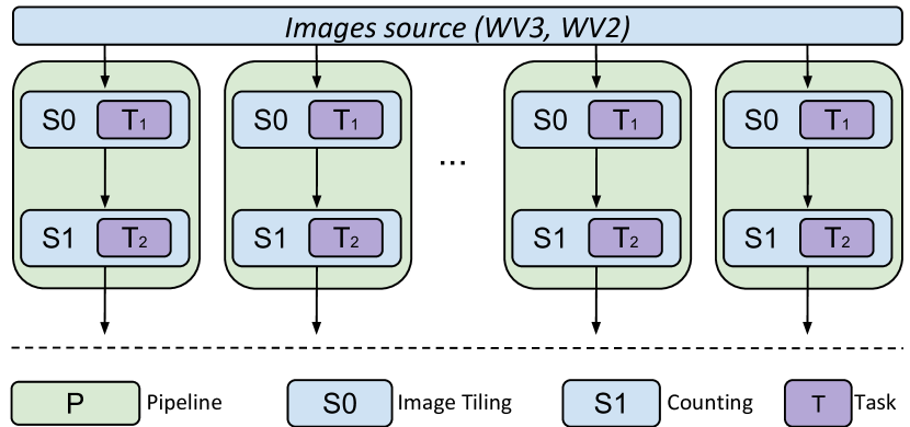
(a)

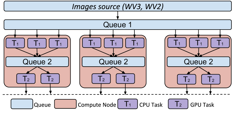
(b)

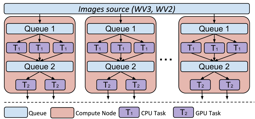
(c)

Figure 1: Design approaches to implement the workflow required for the Seals use case. 1(a)–Design 1: Pipeline, stage and task based design. 1(b)–Design 2: Queue based design with a single queue for all the tiling tasks. 1(c)–Design 2.A: Queue based design with multiple queues for the tiling tasks.

IV-A Design 1: One Image per Pipeline

We specify the workflow for counting the number of seals in a set of images as a set of pipelines. Each pipeline is composed of two stages, each with one type of task. The task of the first stage gets an image as input and generates tiles of that image based on a selected tile size as output. The task of the second stage gets the generated tiles as input, counts the number of seals found in each tile and outputs the aggregated result for the whole image.

Formally, we define two types of tasks:

• $T_{1}=<I,f_{I},t>$, where $I$ is an image, $f_{I}$ is a tiling function and $t$ is a set of tiles that correspond to $I$.

• $T_{2}=<t,f_{A},S>$, where $f_{A}$ is a function that counts seals from a set of tiles and $S$ is the number of seals.

Tiling in $T_{1}$ is implemented with OpenCV [27] and Rasterio [28] in Python. Rasterio allows us to open and convert a GeoTIFF WV3 image to an array. The array is then partitioned to subarrays based on a user-specified scaling factor. Each subarray is converted to an compressed image via OpenCV routines and saved to the filesystem.

Seal counting in $T_{2}$ is performed via a Convolutional Neural Network (CNN) implemented with PyTorch [29]. The CNN counts the number of seals for each tile of an input image. When all tiles are processed, the coordinates of the tiles are converted to the geological coordinates of the image and saved in a file, along with the number of counted seals.

Both tiling and seal counting implementations are invariant between the designs we consider. This is consistent with the designs being task-based, i.e., each task exclusively encapsulates the capabilities required to perform a specific operation over an image or tile. Thus, tasks are independent from the capabilities required to coordinate their execution, whether each task processes a single image or sequence of images.

We implemented Design 1 via EnTK, a workflow engine which exposes an API based on pipelines, stages, and tasks [30]. The user can define a set of pipelines, where each pipeline has a sequence of stages, and each stage has a set of tasks. Stages are executed respecting their order in the pipeline while the tasks in each stage can execute concurrently, depending on resource availability.

For our use case, EnTK has three main advantages compared to other workflow engines: (1) it exposes pipelines and tasks as first-order abstractions implemented in Python; (2) it is specifically designed for concurrent management of up to $10^{5}$ pipelines; and (3) it supports RADICAL-Pilot, a pilot-based runtime system designed to execute heterogeneous bag of tasks on HPC machines [31]. Together, these features address the challenges of heterogeneity, scale and repeatability: users can encode multiple pipelines, each with different types of tasks, executing them at scale on HPC machines without explicitly coding parallelism and resource management.

When implemented in EnTK, the use case workflow maps to a set of pipelines, each with two stages $St_{1}$, $St_{2}$. Each stage has one task $T_{1}$ and $T_{2}$ respectively. The pipeline is defined as $P=(St_{1},St_{2})$. For our use case the workflow consists of $N$ pipelines, where $N$ is the number of images.

Figure 1(a) shows the workflow. For each pipeline, EnTK submits the task of stage $St_{1}$ to the runtime system (RTS). As soon as the task finishes, the task of stage $St_{2}$ is submitted for execution. This design allows concurrent execution of pipelines and, as a result, concurrent analysis of images, one by each pipeline. Since pipelines execute independently and concurrently, there are instances where $St_{1}$ of a pipeline executes at the same time as $St_{2}$ of another pipeline.

Design 1 has the potential to increase utilization of available resources as each compute node of the target HPC machine has multiple CPUs and GPUs. Importantly, computing concurrency comes with the price of multiple reading and writing to the filesystem on which the dataset is stored. This can cause I/O bottlenecks, especially if each task of each pipeline reads from and writes to the same filesystem, possibly over a network connection.

We used a tagged scheduler for EnTK’s RTS to avoid I /O bottlenecks. This scheduler schedules $T_{1}$ of each pipeline on the first available compute node, and guarantees that the respective $T_{2}$ is scheduled on the same compute node. As a result, compute/data affinity is guaranteed among co-located $T_{1}$ and $T_{2}$. While this design avoids I /O bottlenecks, it may reduce concurrency when the performance of the compute nodes and/or the tasks is heterogeneous: $T_{2}$ may have to wait to execute on a specific compute node while another node is free.

IV-B Design 2: Multiple images per pipeline

Design 2 implements a queue-based design. We introduce two tasks $T_{1}$ and $T_{2}$ as defined in §IV-A. In contrast to Design 1, these tasks are bootstrapped once and then executed for as long as resources are available, processing input images at the rate taken to process each image. The number of concurrent $T_{1}$ and $T_{2}$ depends on available resources, including CPUs, GPUs, and RAM.

For the implementation of Design 2, we do not need EnTK, as we submit a bag of $T_{1}$ and $T_{2}$ tasks via the RADICAL-Pilot RTS, and manage the data movement between tasks via queues. As shown in Fig. 1(b), Design 2 uses one queue (Queue 1) for the dataset, and another queue (Queue 2) for each compute node. For each compute node, each $T_{1}$ pulls an image from Queue 1, tiles that image and then queues the resulting tiles to Queue 2. The first available $T_{2}$ on that compute node, pulls those tiles from Queue 2, and counts the seals.

To communicate data and control signals between queues and tasks, we defined a communication protocol with three entities: Sender, Receiver, and Queue. Sender connects to Queue and pushes data. When done, Sender informs Queue and disconnects. Receiver connects to Queue and pulls data. If there are no data in Queue but Sender is connected, Receiver pulls a “wait” message, waits, and pulls again after a second. When there are no data in Queue or Sender is not connected to Queue, Receiver pulls an “empty” message, upon which it disconnects and terminates. This ensures that tasks are executing, even if starving, and that all tasks are gracefully terminating when all images are processed.

Note that Design 2 load balances $T_{1}$ tasks across compute nodes but balances $T_{2}$ tasks only within each node. For example, suppose that $T_{1}$ on compute node $A$ runs two times faster than $T_{1}$ on compute node $B$. Since both tasks are pulling images from the same queue, $T_{1}$ of $A$ will process twice as many images as $T_{1}$ of $B$. Both $T_{1}$ of $A$ and $B$ will execute for around the same amount of time until Queue 1 is empty, but Queue 2 of $A$ will be twice as large as Queue 2 of $B$. $T_{2}$ tasks executing on $B$ will process half as many images as $T_{2}$ tasks on $A$, possibly running for a shorter period of time, depending on the time taken to process each image.

In principle, Design 2 can be modified to load balance also across Queue 2 but in practice, as discussed in §IV-A, this would produce I/O bottlenecks: Load balancing across $T_{2}$ tasks would require for all tiles produced by $T_{1}$ tasks to be written to and read from a filesystem shared across multiple compute nodes. Keeping Queue 2 local to each compute node enables using the filesystem local to each compute node.

IV-B1 Design 2.A: Uniform image dataset per pipeline

The lack of load balancing of $T_{2}$ tasks in Design 2 can be mitigated by introducing a queue in each node from where $T_{1}$ tasks pull images. This allows early binding of images to compute nodes, i.e., deciding the distribution of images per node before executing $T_{1}$ and $T_{2}$. As a result, the execution can be load balanced among all available nodes, depending on the correlation between image properties and image execution time.

Figure 1(c) shows variation 2.A of Design 2. The early binding of images to compute nodes introduces an overhead compared to using late binding via a single queue as in Design 2. Nonetheless, depending on the strength of the correlation between image properties and execution time, design 2.A offers the opportunity to improve resource utilization. While in Design 2 some node may end up waiting for another node to process a much larger Queue 2, in design 2.A this is avoided by guaranteeing that each compute node has an analogous payload to process.

V Experiments and Discussion

We executed three experiments using GPU compute nodes of the XSEDE Bridges supercomputer. These nodes offer 32 cores, 128 GB of RAM and two P100 Tesla GPUs. We stored the dataset of the experiments and the output files on XSEDE Pylon5 Lustre filesystem. We stored the tiles produced by the tailing tasks on the local filesystem of the compute nodes. This way, we avoided creating a performance bottleneck by performing millions of reads and writes of $\approx 700$ KB on Pylon5. We submitted jobs requesting 4 compute nodes to keep the average queue time within a couple of days. Requesting more nodes produced queue times in excess of a week.

The experiments dataset consists of $3,097$ images, ranging from $50$ to $2,770$ MB for a total of $\approx 4$ TB of data. The images size follows a normal distribution with a mean value of $1,304.85$ MB and standard deviation of $512.68$ MB.

For Design 1, 2 and 2.A described in §IV, Experiment 1 models the execution time of the two tasks of our use case as a function of the image size (the only property of the images for which we found a correlation with execution time); Experiment 2 measures the total resource utilization of each design; and Experiment 3 characterizes the overheads of the middleware implementing each design. Together, these experiments enable performance comparison across designs, allowing us to draw conclusions about the performance of heterogeneous task-based execution of data-driven workflows on HPC resources.

V-A Experiment 1: Design 1 Tasks Execution Time

Fig. 2 shows the execution time of the tiling task—defined as $T_{1}$ in §IV-A—as a function of the image size. We partition the set of images based on image size, obtaining 22 bins of $125$ MB each in the range of $[50;2,800]$ MB. The average time taken to tile an image in each bin tends to increase with the size of the image. The box-plots show some positive skew of the data with a number of data points falling outside the assumed normal distribution. There are also large standard deviations ($STD$, blue line) in most of the bins. Thus, there is a weak correlation between task execution time and image size with a large spread across all the image sizes.

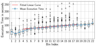
Figure 2: Experiment 1, Design 1: Box-plots of $T_{1}$ execution time, mean and $STD$ for $125$ MB image size bins. Red line shows fitted linear function.

We explored the causes of the observed $STD$ by measuring how it varies in relation to the number of tiling tasks concurrently executing on the same node. Fig. 3 shows the standard deviation of each bin of Fig. 2, based on the amount of used task concurrency. We observe that $STD$ drops with increased concurrency but remains relatively stable between bins $\#6$ and $\#20$. We attribute the initial dropping to how Lustre’s caching improves the performance of an increasing number of concurrent requests. Further, we observe that as the type of task and the compute node are the same across all our measures, the relatively stable and consistent $STD$ observed across degrees of task concurrency depends on fluctuations in the node performance.

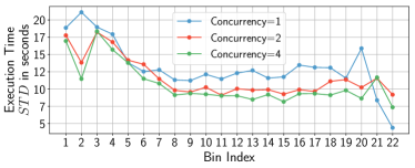
Figure 3: $STD$ of $T_{1}$ execution time based on image size bin and number of concurrent tasks. Mostly dependent on compute node’s performance and invariant across values of task concurrency.

Fig. 2 indicates that the execution time is a linear function of the image size between bin #4 and bin #18. bins $1-3$ and $19-23$ are not representative as the head and tail of the image sizes distribution contain less than $5\%$ of the image dataset. We model the execution time as:

$$T(x)=\alpha\times x+\beta$$ (1)

where $x$ is the image size.

We found the parameter values of Eq. 1 by using a non-linear least squares algorithm to fit our experimental data, which are $\alpha=1.92\times 10^{-2}$, and $\beta=60.49$ (see red line in Fig. 2). $R^{2}$ of our fitting is $0.97$, showing a very good fit of the curve to the actual data.

The Standard Error of the estimation, $S_{error}$, reflects the precision of our regression. The $S_{error}$ is equal to $1.93$, shown as the red shadow in Fig. 2. From $R^{2}$ and $S_{error}$ we conclude that our estimated function is validated and is a good fit for the execution time of $T_{1}$ for Design 1.

Fig. 4 shows the execution time of the seals counting task as a function of the image size. Defined as $T_{2}$ in §IV-A, this task presents a different behavior than $T_{1}$, as the code executed is different. Note the slightly stronger positive skew of the data compared to that of Fig. 2 but still consistent with our conclusion that deviations are mostly due to fluctuations in the compute node performance (i.e., different code but similar fluctuations).

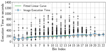
Figure 4: Experiment 1, Design 1: Box-plots of $T_{2}$ execution time, mean and $STD$ for $125$ MB image size bins. Green line shows fitted linear function.

Similar to $T_{1}$, Fig. 4 shows a weak correlation between the execution time of $T_{2}$ and image size. In addition, the variance per bin is relatively similar across bins, as expected based on the analysis of $T_{1}$. The box-plot and the mean execution time indicate that a linear function is a good candidate for a model of $T_{2}$. As in Eq. 1, we fitted a linear function to the execution time as a function of the image size for the same bins as $T_{1}$.

Using the same method we used with $T_{1}$, we produced the green line in Fig. 4 with parameter values $\alpha=5.21\times 10^{-2}$ and $\beta=128.53$. $R^{2}$ is $0.96$, showing a good fit of the line to the actual data, while $S_{error}$ is $5.73$, slightly higher than for $T_{1}$. As a result, we conclude that our estimated function is validated and is a good fit for the execution time of $T_{2}$ for Design 1.

V-B Experiment 1: Design 2 Tasks Execution Time

Fig. 5 shows the execution time of $T_{1}$ as a function of the image size for Design 2. In principle, design differences in middleware that execute tasks as independent programs should not directly affect task execution time. In this type of middleware, task code is independent from that of the middleware: once tasks execute, the middleware waits for each task to return. Nonetheless, in real scenarios with concurrency and heterogeneous tasks, the middleware may perform operations on multiple tasks while waiting for others to return. Accordingly, in Design 2 we observe an execution time variation comparable to that observed with Design 1 but Fig. 5 shows a stronger positive skew of the data in Design 2 than Fig. 2 in Design 1.

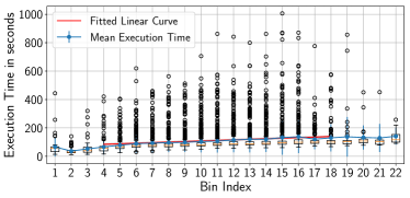
Figure 5: Experiment 1, Design 2: Box-plots of $T_{1}$ execution time, mean and $STD$ for $125$ MB image size bins. Red line shows fitted linear function.

We investigated the positive skew of the data observed in Fig. 5 by comparing the system load of a compute node when executing the same number of tiling tasks in Design 1 and 2. The system load of Design 2 was higher than that of Design 1. Compute nodes have the same hardware and operating system, and run the same type and number of system programs. As we used the same type of task, image and task concurrency, we conclude that the middleware implementing Design 2 uses more compute resources than that used for Design 1. Due to concurrency, the middleware of Design 2 competes for resources with the tasks, momentarily slowing down their execution. This is consistent with the architectural differences across the two designs: Design 2 requires resources to manage queues and data movement while Design 1 has only to schedule and launch tasks on each node.

We fitted Eq. 1 to the execution time of $T_{1}$ for Design 2, obtaining $\alpha=3.174\times 10^{-2}$ and $\beta=64.81$. The fitting produced the red line in Fig. 5. $R^{2}$ is $0.92$, showing a good fit of the curve to the data and $S_{error}$ is $5.50$, validating our estimated function. $R^{2}$ and especially $S_{error}$ are worse compared to Design 1, an expected difference based on the positive skew of the data observed in Design 2.

Fig. 6 shows that Design 2 also produces a much stronger positive skew of $T_{2}$ execution time compared to executing $T_{2}$ with Design 1. $T_{2}$ executes on GPU and $T_{1}$ on CPU but their execution times produce comparable skew in Design 2. This further supports our hypothesis that the long tail of the distribution of $T_{1}$ and especially $T_{2}$ execution times depends on the competition for main memory and I/O between the middleware implementing Design 2 and the executing tasks.

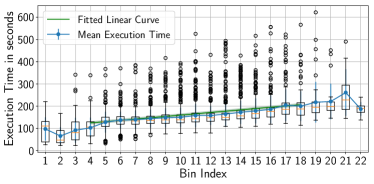
Figure 6: Experiment 1, Design 2: Box-plots of $T_{2}$ execution time, mean and $STD$ for $125$ MB image size bins. Green line shows fitted linear function.

Fitting the model gives $\alpha=4.71\times 10^{-2}$ and $\beta=95.83$. $R^{2}$ is $0.95$ and $S_{error}$ of $5.96$. As a result, the model is validated and a good candidate for the experimental data. We attribute the difference between these values and those of the model of $T_{2}$ for Design 1 to the already described positive skew of execution times in Design 2.

V-B1 Design 2.A

Similarly to the analysis in Design 1 and 2 we fitted data from Design 2.A to Eq. 1. For $T_{1}$ the fit gives $\alpha=2.74\times 10_{-2}$ and $\beta=49.03$, with $R^{2}$ and $S_{error}$ of $0.94$ and $3.89$ respectively. For $T_{2}$ the fit gives $\alpha=4.8\times 10_{-2}$ and $\beta=87.36$, with $R^{2}=0.95$ and $S_{error}=6.19$. Both models are therefore a good fit for the data and are validated.

The results of our experiments indicate that, on average and across multiple runs, there is a decrease in the execution time of $T_{1}$ and an increase in that of $T_{2}$ compared to Design 2. Design 2.A requires one queue more than Design 2 for $T_{1}$ and therefore more resources for Design 2.A implementation. This can explain the slowing of $T_{2}$ but not the speedup of $T_{1}$. This requires further investigation, measuring whether the performance fluctuations of compute nodes are larger than measured so far.

As discussed in §IV-B, balancing of workflow execution differs between Design 2 and Design 2.A. Fig. 7(a) shows that each $T_{1}$ task can work on a different number of images but all $T_{1}$ tasks concurrently execute for a similar duration. The four distributions in Fig. 7(a) also show that this balancing can result in different input distributions for each compute node, affecting the total execution time of $T_{2}$ tasks on each node. Thus, Design 2 can create imbalances in the time to completion of $T_{2}$, as shown by the red bars in Fig. 7(a).

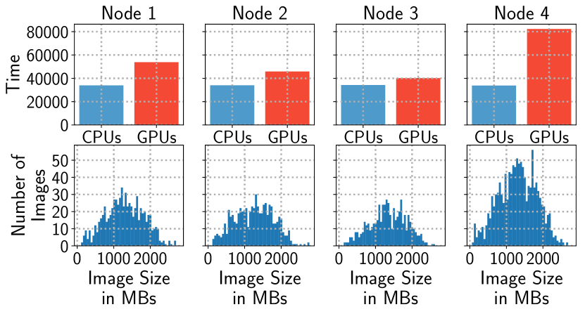
(a)

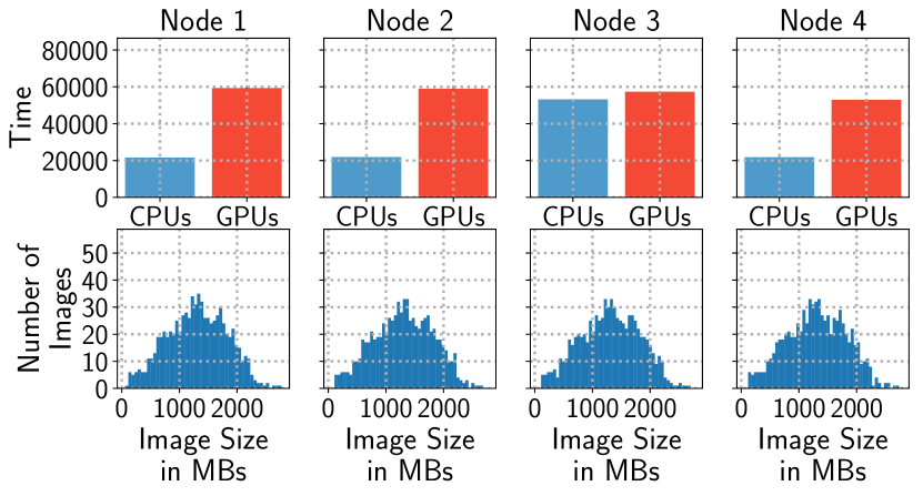
(b)

Figure 7: Execution time of $T_{1}$ (blue) and $T_{2}$ (red), and distributions of image size per node for (a) Design 2 and (b) Design 2.A.

Design 2.A addresses these imbalances by early binding images to compute nodes. Comparing the lower part of Fig. 7(a) and Fig. 7(b) shows the difference between the distributions of image size for each node between Design 2 and 2.A. In Design 2.A, due to the modeled correlation between time to completion and the size of the processed image, the similar distribution of the size of the images bound to each compute node balances the total processing time of the workflow across multiple nodes.

Note that Fig. 7 shows just one of the runs we perform for this experiment. Due to the random pulling of images from a global queue performed by Design 2, each run shows different distributions of image sizes across nodes, leading to large variations in the total execution time of the workflow. Fig. 7(b) shows also an abnormal behavior of one compute node: For images larger than $1.5$GBs, Node 3 CPU performance is markedly slower than other nodes when executing $T_{1}$. Different from Design 2, Design 2.A can balance these fluctuations in $T_{1}$ as far as they don’t starve $T_{2}$ tasks.

V-C Experiment 2: Resource Utilization Across Designs

Resource utilization varies across Design 1, 2 and 2.A. In Design 1, the RTS (RADICAL-Pilot) is responsible for scheduling and executing tasks. $T_{1}$ is memory intensive and, as a consequence, we were able to concurrently execute 3 $T_{1}$ on each compute node, using only 3 of the 32 available cores. We were instead able to execute 2 $T_{2}$ concurrently on each node, using all the available GPUs. Assuming ideal concurrency among the 4 compute nodes we utilized in our experiments, the theoretical maximum utilization per node would be $10.6\%$ for CPUs and $100\%$ for GPUs.

Fig. 8 shows the actual resource utilization, in percent of resource type for each design. The actual CPU utilization of Design 1 (Fig. 8(a)) closely approximates theoretical maximum utilization but GPU utilization is well below the theoretical $100\%$. GPUs are not utilized for almost an hour at the beginning of the execution and utilization decreases to $80\%$ some time after half of the total execution was completed.

Analysis shows that RADICAL-Pilot’s scheduler did not schedule GPU tasks at the start of the execution even if GPU resources were available. This points to an implementation issue and not to an inherent property of Design 1. The drop in GPU utilization is instead explained by noticing that, as explained in §IV, GPU tasks where pinned to specific compute nodes so to avoid I/O bottlenecks. Our experiments confirm that this indeed reduces utilization as some of the GPU tasks on some nodes take longer time to process than those on other nodes.

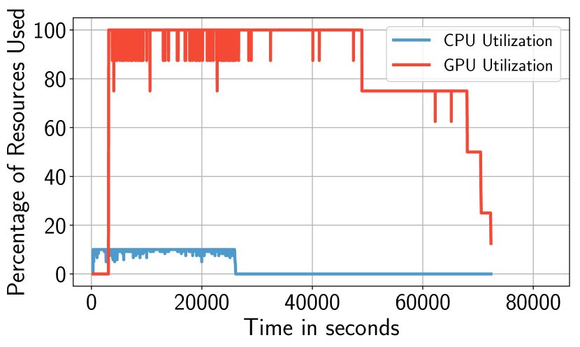
(a)

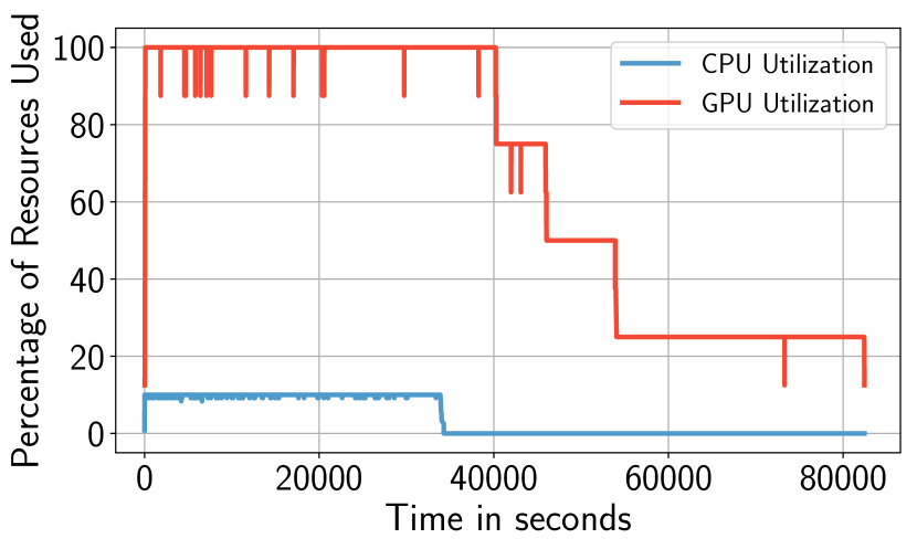
(b)

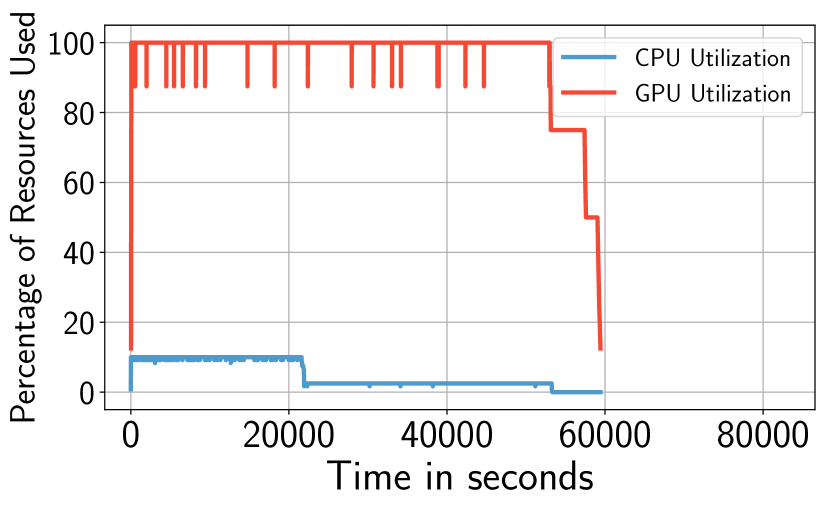
(c)

Figure 8: Percentage of CPU and GPU utilization for: (a) Design 1; (b) Design 2, and (3) Design 2.A.

Fig. 8(b) shows resource utilization for a specific run of Design 2. GPUs are utilized almost immediately as images are becoming available in the queues between $T_{1}$ and $T_{2}$, and this quickly leads to fully utilized resources. CPUs are utilized for more time compared to Design 1, which is expected due to the longer execution times measured and explained in Experiment 1. In addition, two GPUs ($25\%$ GPU utilization) are used for more than $20k$ seconds compared to other GPUs. This shows that the additional execution time of that node was only due to the data size and not due to idle resource time.

Fig. 8(c) shows the resource utilization for a specific run of Design 2.A. For 3 compute nodes out of 4, CPU utilization is shorter than for Design 1 and 2. For the 4th compute node, CPU utilization is much longer as already explained when discussing $T_{1}$ execution time for Node 3 in Fig. 7, Experiment 1. As already mentioned, the anomalous behavior of Node 3 support our hypothesis that compute node performance fluctuations can be much wider than expected.

Fig. 8(c) shows that in Design 2.A GPUs are released faster compared to Design 1 and Design 2, leading to a GPU utilization above $90\%$. As already explained in Experiment 1, this is due to differences in data balancing among designs. This shows the efficacy of two design choices for the concurrent execution of data-driven, compute-intense and heterogeneous workflows: early binding of data to node with balanced distribution of image size alongside the use of local filesystems for data sharing among tasks.

Note that drops in resource utilization are observed in all three designs. In Design 1, although both CPUs and GPUs were used, in some cases CPU utilization dropped to 6 cores. Our analysis showed that this happened when RADICAL-Pilot scheduled both CPU and GPU tasks, pointing to an inefficiency in the scheduler implementation. Design 2 and 2.A CPU utilization drops mostly by one CPU where multiple tiling tasks try to pull from the queue at the same time. This confirm our conclusions in Experiment 1 about resource competition between middleware and executing tasks. In all designs, there is no significant fluctuations in GPU utilization, although there are more often in Design 1 when CPU and GPUs are used concurrently.

V-D Experiment 3: Designs Implementation Overheads

This experiment studies how the total execution time of our use case workflow varies across Design 1, 2 and 2.A. Fig. 9(a) shows that Design 1 and 2 have similar total time to execution within error bars, while Design 2.A improves on Design 2 and both are substantially faster than Design 1. The discussion of Experiment 1 and 2 results explains how these differences relate to the differences in the execution time of $T_{1}$ and $T_{2}$ tasks, and execution concurrency respectively.

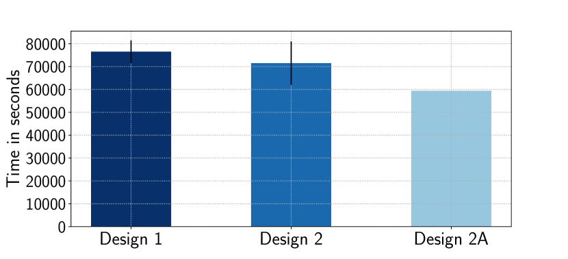
(a)

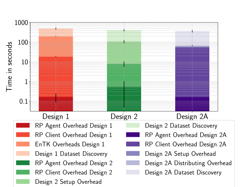
(b)

Figure 9: (a) Total execution time of Design 1, 2 and 2.A. Design 1 and 2 have similar performance, Design 2.A is the fastest. (b) Overheads of Design 1, 2 and 2.A are at least two orders of magnitude less than the total execution time.

Fig. 9(b) shows the overheads of each design implementation. All three designs overheads are at least two orders of magnitude smaller than the total time to execution. A common overheads between all designs is the “Dataset Discovery Overhead”. This overhead is the time needed to list the dataset and it is proportional to the size of the dataset. RADICAL-Pilot has two main components: Agent and Client. RADICAL-Pilot Agent’s overhead is less than a second in all designs while RADICAL-Pilot Client’s overhead is in the order of seconds for all three designs. The latter overhead is proportional to the number of tasks submitted simultaneously to RADICAL-Pilot Agent.

EnTK’s overhead in Design 1 includes the time to: (1) create the workflow consisting of $3.1k$ independent pipelines; (2) start EnTK’s components; and (3) submit the tasks that are ready to be executed to RADICAL-Pilot. This overhead is proportional to the number of tasks in the first stage of a pipeline, and the number of pipelines in the workflow. EnTK does not currently support partial workflow submission, which would allow us to submit the minimum number of tasks to fully utilize the resources before submitting the rest. Experiments should be performed to measure the offset between resource utilization optimization and increased time spent in communicating between EnTK and RADICAL-Pilot.

Fig. 9(b) shows that the dominant overheads of Design 2 is “Design 2 Setup Overhead”. This overhead includes setting up and starting queues in each compute node, and starting and shutting down both $T_{1}$ and $T_{2}$ tasks on each node. Setting up and starting the queues accounts for most of the overhead as we use a conservative waiting time to assure that all the queues are indeed up and ready. This can be optimized further reducing the impact of this overhead.

Alongside the overheads already discussed, Design 2.A also introduces an overhead called “Design 2.A Distributing Overhead” when partitioning and distributing the dataset over separate nodes. The average time of this overhead is $7.5$ seconds, with a standard deviation of $3.71$ and is proportional to the dataset and the number of available compute nodes.

In general, Design 2.A shows the best and more stable performance, in terms of overheads, resource utilization, load balancing and total time to execution. Although Design 2 has similar overheads, even assuming minimization of Setup Overhead, it does not guarantee load balancing as done instead by 2.A. Design 1 separates the execution in independent pipelines that are independently executed by the runtime system on any available resource. Based on the results of our analysis, both EnTK and RADICAL-Pilot can be configured to implement early binding of images to each compute node as done in Design 2.A. Nonetheless, Design 1 would still require executing a task for each image, imposing bootstrap and tear down overheads for each task.

VI Discussion and Conclusion

While design 1, 2 and 2.A can successfully support the execution of the paradigmatic use case described in §III, our experiments show that for the metrics considered, Design 2.A is the one that offers the better overall performance. Generalizing this result, use cases that are both data-driven and compute-intense benefit from early binding of data to compute node so to maximize data and compute affinity and equally balance input across nodes. This approach minimizes the overall time to completion of this type of workflows while maximizing resource utilization.

Our analysis also shows the limits of an approach where pipelines, i.e., compute tasks, are late bound to compute nodes. In program-based designs, the overhead of bootstrapping programs needs to be minimized insuring that each pipeline processes as much input as possible (in our use case, images). In presence of large amount of data, late binding implies copying, replicating or accessing data over network and at runtime. We showed that, in contemporary HPC infrastructures, this is too costly both for resource utilization and total time to completion.

Infrastructure-wise, our experiments show the limits imposed by an unbalance between number of CPU cores and available memory. Given data-driven computation where multi GB images need processing, we were able to use just $10\%$ of the available cores due to the amount of RAM required. This applies also to the unbalance between CPUs and GPUs: use cases with heterogeneous tasks would benefit from a n higher GPU/CPU ratio.

These results apply to the evaluation of the design of existing and future computing frameworks. For example, we will be extending both EnTK and RADICAL-Pilot to implement Design 2.A. We will use our overheads characterization as a baseline to evaluate our production-grade implementation and further improve the efficiency of our middleware. Further, we will apply the presented experimental methodology to other use cases and infrastructures, measuring the trade offs imposed by other types of task heterogeneity, including multi-core or multi-GPU tasks that extends beyond a single compute node.

Beyond design, methodological and implementation insights, the work done with for this paper has already enabled the execution of our use case at unprecedented scale and speed. The $3,097$ images of our dataset can be analyzed in less than 20 hours, compared to labor-intensive weeks previously required on non-HPC resources.

Acknowledgements We thank Andre Merzky (Rutgers) and Brad Spitzbart (Stony Brook) for useful discussions. This work is funded by NSF EarthCube Award Number 1740572. Computational resources were provided by NSF XRAC awards TG-MCB090174. We thank the PSC Bridges PI and Support Staff for supporting this work through resource reservations.

Software and Data Source Scripts: http://github.com/iceberg-project/Seals/, Experiments and Data:http://github.com/radical-experiments/iceberg_seals/

References

- [1] Hoang Vo, Jun Kong, Dejun Teng, Yanhui Liang, Ablimit Aji, George Teodoro, and Fusheng Wang. Mareia: a cloud mapreduce based high performance whole slide image analysis framework. Distributed and Parallel Databases, Jul 2018.
- [2] Matei Zaharia, Mosharaf Chowdhury, Michael J. Franklin, Scott Shenker, and Ion Stoica. Spark: Cluster computing with working sets. In Proceedings of the 2Nd USENIX Conference on Hot Topics in Cloud Computing, HotCloud’10, pages 10–10, Berkeley, CA, USA, 2010. USENIX Association.
- [3] Zhao Zhang, Kyle Barbary, Frank A. Nothaft, Evan R. Sparks, Oliver Zahn, Michael J. Franklin, David A. Patterson, and Saul Perlmutter. Kira: Processing Astronomy Imagery Using Big Data Technology. IEEE Transactions on Big Data, pages 1–1, 2016.
- [4] Yuzhong Yan and Lei Huang. Large-Scale Image Processing Research Cloud. 2014.
- [5] Raul Ramos-Pollan, Fabio A. Gonzalez, Juan C. Caicedo, Angel Cruz-Roa, Jorge E. Camargo, Jorge A. Vanegas, Santiago A. Perez, Jose David Bermeo, Juan Sebastian Otalora, Paola K. Rozo, and John E. Arevalo. BIGS: A framework for large-scale image processing and analysis over distributed and heterogeneous computing resources. In 2012 IEEE 8th International Conference on E-Science, pages 1–8. IEEE, oct 2012.
- [6] Daniel E J Hobley, Jordan M Adams, Sai Siddhartha Nudurupati, Eric W H Hutton, Nicole M Gasparini, and Gregory E Tucker. Creative computing with Landlab: an open-source toolkit for building, coupling, and exploring two-dimensional numerical models of Earth-surface dynamics. Earth Surf. Dynam, 5:21–46, 2017.
- [7] Antonella Galizia, Daniele D’Agostino, and Andrea Clematis. An MPI–CUDA library for image processing on HPC architectures. Journal of Computational and Applied Mathematics, 273:414–427, jan 2015.
- [8] Amir Gholami, Andreas Mang, Klaudius Scheufele, Christos Davatzikos, Miriam Mehl, and George Biros. A framework for scalable biophysics-based image analysis. In Proceedings of the International Conference for High Performance Computing, Networking, Storage and Analysis, SC ’17, pages 19:1–19:13, New York, NY, USA, 2017. ACM.
- [9] Yuankai Huo, Justin Blaber, Stephen M. Damon, Brian D. Boyd, Shunxing Bao, Prasanna Parvathaneni, Camilo Bermudez Noguera, Shikha Chaganti, Vishwesh Nath, Jasmine M. Greer, Ilwoo Lyu, William R. French, Allen T. Newton, Baxter P. Rogers, and Bennett A. Landman. Towards portable large-scale image processing with high-performance computing. Journal of Digital Imaging, 31(3):304–314, Jun 2018.
- [10] Stephen M Damon, Brian D Boyd, Andrew J Plassard, Warren Taylor, and Bennett A Landman. DAX - The Next Generation: Towards One Million Processes on Commodity Hardware. Proceedings of SPIE–the International Society for Optical Engineering, 2017, 2017.
- [11] Rafael Vescovi, Ming Du, Vincent de Andrade, William Scullin, Gürsoy Doğa, and Chris Jacobsen. Tomosaic: efficient acquisition and reconstruction of teravoxel tomography data using limited-size synchrotron X-ray beams. Journal of Synchrotron Radiation, 25:1478–1489, aug 2018.
- [12] Steve Petruzza, Aniketh Venkat, Attila Gyulassy, Giorgio Scorzelli, Frederick Federer, Alessandra Angelucci, Valerio Pascucci, and Peer-Timo Bremer. Isavs: Interactive scalable analysis and visualization system. In SIGGRAPH Asia 2017 Symposium on Visualization, SA ’17, pages 18:1–18:8, New York, NY, USA, 2017. ACM.
- [13] George Teodoro, Tony Pan, Tahsin M. Kurc, Jun Kong, Lee A.D. Cooper, Norbert Podhorszki, Scott Klasky, and Joel H. Saltz. High-throughput Analysis of Large Microscopy Image Datasets on CPU-GPU Cluster Platforms. In 2013 IEEE 27th International Symposium on Parallel and Distributed Processing, pages 103–114. IEEE, may 2013.
- [14] Richard Grunzke, Florian Jug, Bernd Schuller, René Jäkel, Gene Myers, and Wolfgang E. Nagel. Seamless HPC Integration of Data-Intensive KNIME Workflows via UNICORE. pages 480–491. Springer, Cham, 2017.
- [15] Krzysztof Benedyczak, Bernd Schuller, Maria Petrova-El Sayed, Jedrzej Rybicki, and Richard Grunzke. UNICORE 7 — Middleware services for distributed and federated computing. In 2016 International Conference on High Performance Computing & Simulation (HPCS), pages 613–620. IEEE, jul 2016.
- [16] K Ullas Karanth. Estimating tiger panthera tigris populations from camera-trap data using capture—recapture models. Biological conservation, 71(3):333–338, 1995.
- [17] David Western, Rosemary Groom, and Jeffrey Worden. The impact of subdivision and sedentarization of pastoral lands on wildlife in an african savanna ecosystem. Biological Conservation, 142(11):2538–2546, 2009.
- [18] Heather J. Lynch, Richard White, Andrew D. Black, and Ron Naveen. Detection, differentiation, and abundance estimation of penguin species by high-resolution satellite imagery. Polar Biology, 35(6):963–968, Jun 2012.
- [19] Benjamin Kellenberger, Diego Marcos, and Devis Tuia. Detecting mammals in uav images: Best practices to address a substantially imbalanced dataset with deep learning. Remote Sensing of Environment, 216:139 – 153, 2018.
- [20] Andrei Polzounov, Ilmira Terpugova, Deividas Skiparis, and Andrei Mihai. Right whale recognition using convolutional neural networks. CoRR, abs/1604.05605, 2016.
- [21] Mohammad Sadegh Norouzzadeh, Anh Nguyen, Margaret Kosmala, Alexandra Swanson, Meredith S. Palmer, Craig Packer, and Jeff Clune. Automatically identifying, counting, and describing wild animals in camera-trap images with deep learning. Proceedings of the National Academy of Sciences, 115(25):E5716–E5725, 2018.
- [22] Adriana Fabra and Virginia Gascón. The convention on the conservation of antarctic marine living resources (ccamlr) and the ecosystem approach. The International Journal of Marine and Coastal Law, 23(3):567–598, 2008.
- [23] Helmut Hillebrand, Thomas Brey, Julian Gutt, Wilhelm Hagen, Katja Metfies, Bettina Meyer, and Aleksandra Lewandowska. Climate change: Warming impacts on marine biodiversity. In Handbook on Marine Environment Protection, pages 353–373. Springer, 2018.
- [24] Keith Reid. Climate change impacts, vulnerabilities and adaptations: Southern ocean marine fisheries. Impacts of climate change on fisheries and aquaculture, page 363, 2019.
- [25] Olaf Ronneberger, Philipp Fischer, and Thomas Brox. U-net: Convolutional networks for biomedical image segmentation. In International Conference on Medical image computing and computer-assisted intervention, pages 234–241. Springer, 2015.
- [26] Diederik P Kingma and Jimmy Ba. Adam: A method for stochastic optimization. arXiv preprint arXiv:1412.6980, 2014.
- [27] G. Bradski. The OpenCV Library. Dr. Dobb’s Journal of Software Tools, 2000.
- [28] Sean Gillies et al. Rasterio: geospatial raster i/o for Python programmers, 2013–.
- [29] Adam Paszke, Sam Gross, Soumith Chintala, Gregory Chanan, Edward Yang, Zachary DeVito, Zeming Lin, Alban Desmaison, Luca Antiga, and Adam Lerer. Automatic differentiation in pytorch. In NIPS-W, 2017.
- [30] Vivek Balasubramanian, Matteo Turilli, Weiming Hu, Matthieu Lefebvre, Wenjie Lei, Ryan Modrak, Guido Cervone, Jeroen Tromp, and Shantenu Jha. Harnessing the power of many: Extensible toolkit for scalable ensemble applications. In 2018 IEEE International Parallel and Distributed Processing Symposium (IPDPS), pages 536–545. IEEE, 2018.
- [31] Andre Merzky, Matteo Turilli, Manuel Maldonado, Mark Santcroos, and Shantenu Jha. Using pilot systems to execute many task workloads on supercomputers. In Workshop on Job Scheduling Strategies for Parallel Processing, pages 61–82. Springer, 2018.