Moiré phonons in the twisted bilayer graphene

Abstract

We study the in-plane acoustic phonons in twisted bilayer graphenes using the effective continuum approach. We calculate the phonon modes by solving the continuum equation of motion for infinitesimal vibration around the static relaxed state with triangular domain structure. We find that the moiré interlayer potential only affects the in-plane asymmetric modes, where the original linear dispersion is broken down into miniphonon bands separated by gaps, while the in-plane symmetric modes with their linear dispersion are hardly affected. The phonon wave functions of asymmetric modes are regarded as collective vibrations of the domain-wall network, and the low-energy phonon band structure can be qualitatively described by an effective moiré-scale lattice model.

I Introduction

Twisted bilayer graphene (TBG), or a pair of graphene layers rotationally stacked on top of each otherBerger et al. (2006); Hass et al. (2007, 2008); Li et al. (2009); Miller et al. (2010); Luican et al. (2011), exhibits a variety of physical properties depending on the twist angle $\theta$. In a small $\theta$, in particular, a long-period moiré pattern due to a slight lattice mismatch folds the Dirac cone of graphene into a superlattice Brillouin zone Lopes dos Santos et al. (2007); Mele (2010); Trambly de Laissardière et al. (2010); Shallcross et al. (2010); Morell et al. (2010); Bistritzer and MacDonald (2011); Kindermann and First (2011); Xian et al. (2011); Lopes dos Santos et al. (2012); Moon and Koshino (2012); de Laissardiere et al. (2012); Moon and Koshino (2013); Weckbecker et al. (2016), and nearly-flat bands with extremely narrow band width emerge at some particular $\theta$’s called the magic angles. The discovery of the superconductivity and strongly correlated insulating state in the magic-angle TBGs Cao et al. (2018a, b); Yankowitz et al. (2019) has attracted enormous attention to this system.

While the early theoretical studies on TBG simply assumed a stack of rigid graphene layers without deformation, the actual TBG spontaneously relaxes to the energetically favorable lattice structure. There the in-plane distortion maximizes the area of AB stacking (graphite’s Bernal stacking) to form a triangular domain pattern Popov et al. (2011); Brown et al. (2012); Lin et al. (2013); Alden et al. (2013); van Wijk et al. (2015); Dai et al. (2016); Jain et al. (2016); Nam and Koshino (2017); Carr et al. (2018); Lin et al. (2018); Yoo et al. (2019); Walet and Guinea (2019), and at the same time the out-of-plane distortion leads to a corrugation of graphene layers Uchida et al. (2014); van Wijk et al. (2015); Lin et al. (2018). The electronic band structure is also significantly affected by the lattice relaxation Nam and Koshino (2017); Lin et al. (2018); Koshino et al. (2018); Yoo et al. (2019); Walet and Guinea (2019); Lucignano et al. (2019). A similar structural relaxation was also observed in moiré superlattice of graphene and hexagonal boron-nitride (h-BN)Woods et al. (2014), and the effects on the band structure were investigated San-Jose et al. (2014a, b); Jung et al. (2015).

The lattice deformation of the moiré superlattice is expected to significantly influence the phonon properties. In the intrinsic graphene, the low-energy phonon spectrum is composed of transverse acoustic (TA) modes and longitudinal acoustic (LA) modes which have linear dispersions, and the out-of-plane flexural phonons (ZA) with a quadratic dispersion Grüneis et al. (2002); Suzuura and Ando (2002); Yan et al. (2008). In the AB-stacked bilayer graphene, the phonon modes of the top layer and the bottom layer are coupled to form layer-symmetric and asymmetric modes Yan et al. (2008); Nika and Balandin (2017). The phonon spectrum of TBG was calculated by fully taking account of all the atoms in the moiré unit cells Jiang et al. (2012); Cocemasov et al. (2013); Choi and Choi (2018); Angeli et al. (2019), where the phonon density of states is found to be close to that of the regular AB-stacked bilayer graphene insensitively to the twist angle. On the other hand, it is naturally expected that the moiré interlayer potential would cause superlattice zone-folding and miniband generation in the phonon spectrum. So far such zone-folding effect was argued for graphene h-BN superlattice Felix and Pereira (2018) and very recently for the optical branch of TBG Angeli et al. (2019). The low frequency phonon minibands in the TBGs are not thoroughly understood although they may have important roles for low-energy transport and collective phenomena Choi and Choi (2018); Wu et al. (2018, 2019).

In this paper, we study the in-plane acoustic phonons in TBG and investigate the effects of the moiré superlattice structure on the phonon spectrum. The calculation is based on the continuum approach using the elastic theory and the registry-dependent interlayer potential, which was used to obtain the relaxed lattice structure with a triangular domain pattern Nam and Koshino (2017). We derive the phonon modes by solving the continuum equation of motion for infinitesimal vibration around the static relaxed state. We find that the moiré interlayer potential couples only to the in-plane asymmetric modes (i.e., the top and bottom layers slide in the opposite directions parallel to the graphene layers), while the in-plane symmetric modes (which slide in the same direction) are hardly affected. In the in-plane asymmetric modes, the original linear dispersion is broken into miniphonon bands separated by gaps, where the phonon wave functions are regarded as collective vibrations of the nano-scale triangular lattice of AB- and BA-stacking domains. The formation of miniphonon bands and gaps is more pronounced in lower twist angles. We find that the phonon band structure in the low twist angles becomes nearly invariant when renormalized by the energy scale inversely proportional to the moiré superlattice period. The universal behavior of the moiré phonon bands can be understood by an effective moiré-scale lattice model.

II Methods

Figure 1: (a) Non-relaxed atomic structure of TBG with $\theta=3.89^{\circ}$. AA spots are located at the crossing points of the grid lines. (b) First Brillouin zone of TBG.

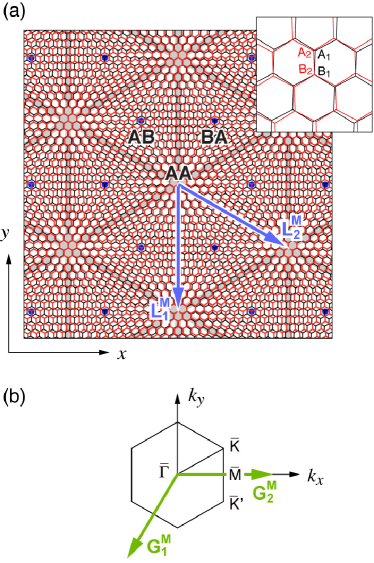
We consider a TBG lattice with a relatively small twist angle $\theta$ lower than a few degree, as shown in Fig. 1(a). Here we define the geometry of TBG by starting from perfectly overlapping honeycomb lattices and rotating the layer 1 and 2 by $-\theta/2$ and $+\theta/2$, respectively. We define $\mathbf{a}_{1}^{(0)}=a(1,0)$ and $\mathbf{a}_{2}^{(0)}=a(1/2,\sqrt{3}/2)$ as the primitive lattice vectors of the initial bilayer graphene before the rotation, where $a\approx 0.246\,\mathrm{nm}$ is the graphene’s lattice constant. Then the lattice vectors of layer 1 are given by $\mathbf{a}_{i}=R(-\theta/2)\mathbf{a}_{i}^{(0)}$ and those of layer 2 are given by $\tilde{\mathbf{a}}_{i}=R(\theta/2)\mathbf{a}_{i}^{(0)}$ ($i=1,2$), where $R(\phi)$ represents the rotation matrix by angle $\phi$. The corresponding reciprocal lattice vectors, $\mathbf{a}^{*}_{i}$ and $\tilde{\mathbf{a}}^{*}_{i}$ for layer 1 and 2, respectively, are defined by $\mathbf{a}_{i}\cdot\mathbf{a}^{*}_{j}=2\pi\delta_{ij}$ and $\tilde{\mathbf{a}}_{i}\cdot\tilde{\mathbf{a}}^{*}_{j}=2\pi\delta_{ij}$.

When the twist angle is small, the slight mismatch of the lattice periods of two layers gives rise to a long-period moiré beating pattern. The primitive lattice vector of the moiré superlattice $\mathbf{L}_{i}^{\rm M}$ is given by Nam and Koshino (2017)

$$\mathbf{L}_{i}^{\rm M}=[1-R(-\theta)]^{-1}\mathbf{a}_{i}\quad(i=1,2).$$ (1)

The lattice constant $L_{\rm M}=|\mathbf{L}_{1}^{\rm M}|=|\mathbf{L}_{2}^{\rm M}|$ becomes

$$L_{\rm M}=\frac{a}{2\sin(\theta/2)}.$$ (2)

The corresponding moiré reciprocal lattice vectors satisfying $\mathbf{G}^{\rm M}_{i}\cdot\mathbf{L}_{j}^{\rm M}=2\pi\delta_{ij}$ are written as

$$\mathbf{G}_{i}^{\rm M}=[1-R(\theta)]\,\textbf{a}^{*}_{i}=\textbf{a}^{*}_{i}-\tilde{\textbf{a}}^{*}_{i}.\quad(i=1,2).$$ (3)

The first Brillouin zone defined by $\mathbf{G}^{\rm M}_{i}$ is shown in Fig. 1(b). The local structure of TBG approximates the nonrotated bilayer graphene with the in-plane translation. It is characterized by the interlayer sliding vector, or the shift of layer 2’s atom at $\mathbf{r}$, measured from its counterpart on layer 1. Without the lattice relaxation, the interlayer sliding vector is given by

$$\bm{\delta}_{0}(\textbf{r})=\textbf{r}-\textbf{r}_{0}=[1-R(-\theta)]\textbf{r}.$$ (4)

Now we introduce the in-plane lattice vibration specified by the time-dependent displacement vector, $\textbf{u}^{(l)}(\textbf{r},t)$ for layer $l=1,2$. The interlayer sliding vector under the deformation is

$$\bm{\delta}(\textbf{r},t)=\bm{\delta}_{0}(\textbf{r})+\textbf{u}^{(2)}(\textbf{r},t)-\textbf{u}^{(1)}(\textbf{r},t).$$ (5)

Here we concentrate on the in-plane displacement, while the qualitative argument of out-of-plane phonon modes will be presented in Sec. IV. The inter-layer binding energy of TBG is written as

$$U_{B} = \int V[\bm{\delta}(\textbf{r},t)]\text{d}^{2}\textbf{r},$$ (6)

where $V[\bm{\delta}]$ is the interlayer binding energy per area of nonrotated bilayer graphene with the sliding vector $\bm{\delta}$ Nam and Koshino (2017). It can be approximately written as

$$V[\bm{\delta}]=\sum^{3}_{j=1}2V_{0}\cos[\textbf{a}^{*}_{j}\cdot\bm{\delta}],$$ (7)

where $\textbf{a}^{*}_{3}=-\textbf{a}^{*}_{1}-\textbf{a}^{*}_{2}$. The function takes the maximum value $6V_{0}$ at AA stacking ($\bm{\delta}=0$) and the minimum value $-3V_{0}$ at AB and BA stacking. The difference between the binding energies of AA and AB/BA structure is $9V_{0}$ per area, and this amounts to $\Delta\epsilon=9V_{0}S_{G}/4$ per atom where $S_{G}$ is the area of graphene’s unit cell. In the following calculation, we use $\Delta\epsilon=0.0189$ (eV/atom) as a typical value Lebedeva et al. (2011); Popov et al. (2011). By using Eqs. (5) and (7), we have

$$V[\bm{\delta}(\textbf{r},t)]=\sum^{3}_{j=1}2V_{0}\cos[\textbf{G}_{j}^{\rm M}\cdot\textbf{r}+\textbf{a}^{*}_{j}\cdot(\textbf{u}^{(2)}-\textbf{u}^{(1)})],$$ (8)

where $\textbf{G}^{\rm M}_{3}=-\textbf{G}^{\rm M}_{1}-\textbf{G}^{\rm M}_{2}$ and we used the relation $\textbf{a}^{*}_{j}\cdot\bm{\delta}_{0}(\textbf{r})=\textbf{G}_{j}^{\rm M}\cdot\textbf{r}$.

The elastic energy of strained TBG is expressed by Suzuura and Ando (2002); San-Jose et al. (2014b)

$$U_{E}=\sum_{l=1}^{2}\int\frac{1}{2}\left\{(\lambda+\mu)(u_{xx}^{(l)}+u_{yy}^{(l)})^{2}\right.$$

$$\left.+\mu\left[(u_{xx}^{(l)}-u_{yy}^{(l)})^{2}+4(u_{xy}^{(l)})^{2}\right]\right\}d^{2}\textbf{r},$$ (9)

where $\lambda\approx 3.25$ eV/$\text{\AA}^{2}$ and $\mu\approx 9.57$ eV/$\text{\AA}^{2}$ are graphene’s $\text{Lam}\acute{\text{e}}$ factors Zakharchenko et al. (2009); Jung et al. (2015), and $u^{(l)}_{ij}=(\partial_{i}u_{j}^{(l)}+\partial_{j}u_{i}^{(l)})/2$ is the strain tensor. Lastly, the kinetic energy due to the motion of the lattice is expressed as

$$T=\sum_{l=1}^{2}\int\frac{\rho}{2}\left[\dot{u}_{x}^{(l)2}+\dot{u}_{y}^{(l)2}\right]d^{2}\textbf{r},$$ (10)

where $\rho=7.61\times 10^{-7}$ kg/m² is the area density of single-layer graphene, and $\dot{u_{i}}$ represents the time derivative of $u_{i}\,(i=x,y)$.

The Lagrangian of the system is given by $L=T-(U_{E}+U_{B})$ as a functional of $\textbf{u}^{(l)}(\textbf{r})$. We define $\textbf{u}^{\pm}=\textbf{u}^{(2)}\pm\textbf{u}^{(1)}$ and rewrite $L$ as a functional of $\textbf{u}^{\pm}$. The Euler-Lagrange equations for $\textbf{u}^{-}$ read

$$\frac{1}{2}(\lambda+\mu)\left(\frac{\partial^{2}u^{-}_{x}}{\partial x^{2}}+\frac{\partial^{2}u^{-}_{y}}{\partial x\partial y}\right)+\frac{\mu}{2}\left(\frac{\partial^{2}u^{-}_{x}}{\partial x^{2}}+\frac{\partial^{2}u^{-}_{x}}{\partial y^{2}}\right)\\ +\sum_{j=1}^{3}2V_{0}\sin[\textbf{G}_{j}^{\rm M}\cdot\textbf{r}+\textbf{a}^{*}_{j}\cdot\textbf{u}^{-}]a^{*}_{jx}=\frac{1}{2}\rho\ddot{u}^{-}_{x},$$ (11)

$$\frac{1}{2}(\lambda+\mu)\left(\frac{\partial^{2}u^{-}_{y}}{\partial y^{2}}+\frac{\partial^{2}u^{-}_{x}}{\partial x\partial y}\right)+\frac{\mu}{2}\left(\frac{\partial^{2}u^{-}_{y}}{\partial x^{2}}+\frac{\partial^{2}u^{-}_{y}}{\partial y^{2}}\right)\\ +\sum_{j=1}^{3}2V_{0}\sin[\textbf{G}_{j}^{\rm M}\cdot\textbf{r}+\textbf{a}^{*}_{j}\cdot\textbf{u}^{-}]a^{*}_{jy}=\frac{1}{2}\rho\ddot{u}^{-}_{y},$$ (12)

where $a^{*}_{jl}\,(l=x,y)$ is the $l$-component of $\mathbf{a}^{*}_{j}$. The equation of motion for $\textbf{u}^{+}$ is given by replacing $\textbf{u}^{-}$ with $\textbf{u}^{+}$ and removing all the terms including $V_{0}$ in Eqs. (11) and (12). Here the potential terms with $V_{0}$ vanish because $U_{B}$ is not dependent on $\textbf{u}^{+}$ and then the force term $\partial U_{B}/\partial\textbf{u}^{+}$ is zero. Therefore, the mode $\textbf{u}^{+}$ is just equivalent to the original acoustic phonon of graphene.

For $\textbf{u}^{-}$, we consider a small vibration around the static equilibrium state, or

$$\textbf{u}^{-}(\mathbf{r},t)=\textbf{u}^{-}_{0}(\mathbf{r})+\delta\textbf{u}^{-}(\mathbf{r},t).$$ (13)

Here $\textbf{u}^{-}_{0}(\mathbf{r})$ is the static solution of Eqs. (11) and (12), i.e., the optimized relaxed state to minimize $U_{B}+U_{E}$, and $\delta\textbf{u}^{-}(\mathbf{r},t)$ is the perturbational excitation around $\textbf{u}^{-}_{0}$. We define the Fourier components as

$$\textbf{u}_{0}^{-}(\textbf{r})=\sum_{\textbf{G}}\textbf{u}^{-}_{0,\textbf{G}}e^{i\textbf{G}\cdot\textbf{r}},$$ (14)

$$\delta\textbf{u}^{-}(\textbf{r},t)=e^{-i\omega t}\sum_{\textbf{q}}\delta\textbf{u}^{-}_{\textbf{q}}e^{i\textbf{q}\cdot\textbf{r}},$$ (15)

$$\sin\left[\textbf{G}_{j}^{\rm M}\cdot\textbf{r}+\textbf{a}^{*}_{j}\cdot\textbf{u}^{-}_{0}(\textbf{r})\right]=\sum_{\textbf{G}}f^{j}_{\textbf{G}}e^{i\textbf{G}\cdot\textbf{r}},$$ (16)

$$\cos\left[\textbf{G}_{j}^{\rm M}\cdot\textbf{r}+\textbf{a}^{*}_{j}\cdot\textbf{u}^{-}_{0}(\textbf{r})\right]=\sum_{\textbf{G}}h^{j}_{\textbf{G}}e^{i\textbf{G}\cdot\textbf{r}},$$ (17)

where $\textbf{G}=m\textbf{G}^{\rm M}_{1}+n\textbf{G}^{\rm M}_{2}$ are moiré reciprocal vectors and $\omega$ is the phonon frequency.

From Eqs. (11) and (12), the equation for the static solution $\textbf{u}_{0}^{-}$ is given by Nam and Koshino (2017)

$$\textbf{u}^{-}_{0,\textbf{G}}=\sum_{j=1}^{3}4V_{0}f^{j}_{\textbf{G}}\hat{K}_{\textbf{G}}^{-1}\textbf{a}^{*}_{j},$$

$$\hat{K}_{\textbf{G}}=\left({\begin{array}[]{cc}(\lambda+2\mu)G_{x}^{2}+\mu G_{y}^{2}&(\lambda+\mu)G_{x}G_{y}\\ (\lambda+\mu)G_{x}G_{y}&(\lambda+2\mu)G_{y}^{2}+\mu G_{x}^{2}\end{array}}\right).$$ (20)

The equation of motion for the dynamical perturbation part is written as

$$\rho\,\omega^{2}\delta\textbf{u}^{-}_{\textbf{G}+\textbf{q}}=\hat{K}_{\textbf{G}+\textbf{q}}\delta\textbf{u}^{-}_{\textbf{G}+\textbf{q}}-4V_{0}\sum_{\textbf{G}^{\prime}}\hat{V}_{\textbf{G}-\textbf{G}^{\prime}}\delta\textbf{u}^{-}_{\textbf{G}^{\prime}+\textbf{q}},$$

$$\hat{V}_{\textbf{G}}=\sum_{j=1}^{3}h^{j}_{\textbf{G}}\begin{pmatrix}a^{*}_{jx}a^{*}_{jx}&a^{*}_{jx}a^{*}_{jy}\\ a^{*}_{jx}a^{*}_{jy}&a^{*}_{jy}a^{*}_{jy}\end{pmatrix}.$$ (21)

We first derive the static solution $\textbf{u}_{0}^{-}$ by solving a set of the self-consistent equations, Eqs. (14), (16) and (20), by numerical iterations Nam and Koshino (2017). Using the obtained $\textbf{u}_{0}^{-}$, we solve the eigenfunction Eq. (21), to obtain eigenvalues $\omega^{2}$ and the phonon modes $\delta\textbf{u}^{-}$ as a function of $\mathbf{q}$ in the moiré Brillouin zone. Throughout the calculation, we set the $k$-space cut-off for the Fourier components of $\textbf{u}_{0}^{-}$ and $\delta\textbf{u}^{-}$, which is sufficiently large for convergence.

Figure 2: Phonon dispersions of in-plane asymmetric modes ($\mathbf{u}^{-}$) in various twist angles $\theta$. The horizontal axis is scaled by the superlattice Brillouin zone size $\propto 1/L_{M}$, and the vertical axis is scaled by $\omega_{0}\propto 1/L_{M}$ (see the text). (a) Phonon dispersion when the moiré interlayer coupling is absent.

Figure 3: Two-dimensional dispersions of the lowest five modes of in-plane asymmetric vibration ($\mathbf{u}^{-}$) in (a) $\theta=2.65^{\circ}$, (b) 2.20^∘ and (c) 0.547^∘.

Figure 4: Phonon wave functions of the lowest five modes at $\mathbf{q}=(0,2\pi/(6L_{M}))$ in TBG of $\theta=1.05^{\circ}$. The $y$ axis is taken as the horizontal axis, and the color code represents the local binding energy $V[\mbox{\boldmath$\delta$}(\mathbf{r},t)]$ at a certain $t$. Dashed lines indicate the superlattice without vibrations. The corresponding band structure is shown in Fig. 2(d).

Figure 5: (a) Width of the gap (in meV) between the second and the third branches of $\mathbf{u}^{-}$ phonon modes, plotted against the twist angle. The blue dashed line is a guide to the eye indicating the linear dependence on $\theta$. (b) Group velocities (in units of $\sqrt{\lambda/\rho}$, long wavelength limit) of the first and the second $\mathbf{u}^{-}$ phonon modes, plotted against the twist angle. Horizontal dashed lines indicate the velocities of the transverse ($v_{T}$) and longitudinal ($v_{L}$) acoustic phonons in single layer graphene.

Figure 6: Schematics of the domain structure in TBG. The shaded region indicates the domain walls separating AB and BA regions.

Figure 7: (a) Phonon dispersions of the effective lattice model (black solid) and the original model for $\theta=0.547^{\circ}$ from Fig. 2(f) (blue dashed). (b) Phonon vibration of the effective lattice for the first and the second modes at $\mathbf{q}=(0,2\pi/(6L_{M}))$, which are indicated by dots in panel (a). Orange dashed lines indicate the lattice without vibrations.

III Phonon modes

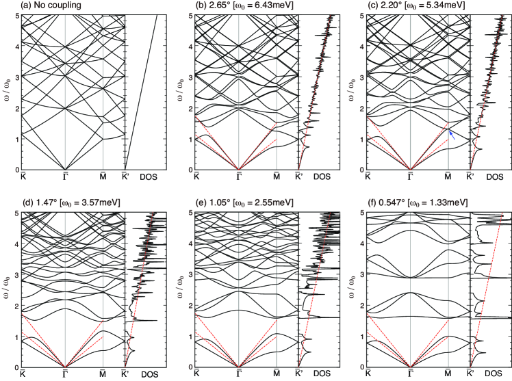
Figure 2 shows the phonon dispersions of in-plane asymmetric modes ($\mathbf{u}^{-}$) calculated for various twist angle $\theta$’s. Here the horizontal axis is the scaled by the superlattice Brillouin zone size ($\propto 2\pi/L_{M}$) and the vertical axis is scaled by

$$\omega_{0}=\sqrt{\frac{\lambda}{\rho}}\frac{2\pi}{L_{M}},$$ (22)

where $\sqrt{\lambda/\rho}$ is the characteristic velocity scale for the acoustic phonons in graphene. Figure 2(a) is the phonon dispersion when the moiré interlayer coupling is absent. This is equivalent to the folded dispersion of intrinsic TA and LA phonons of graphene, which are $\omega(\mathbf{q})=v_{T}q$ and $v_{L}q$, respectively, where $v_{T}=\sqrt{\mu/\rho}$ and $v_{L}=\sqrt{(\lambda+2\mu)/\rho}$.Suzuura and Ando (2002) Figure 2(a) is independent of the twist angle, since both the horizontal and vertical axes are normalized by units proportional to $1/L_{M}$. The same dispersions are also indicated by red dashed lines in Figs. 2(b)-(f). Note that the phonon band structures of in-plane symmetric modes ($\mathbf{u}^{+}$) remain intact and ungapped. So, they are not drawn in this figure or hereafter.

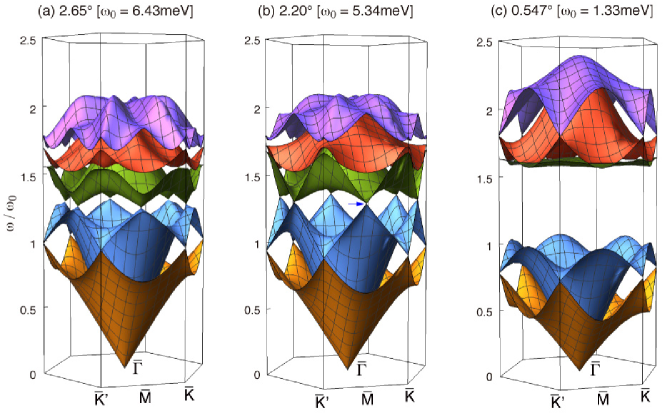
For $\mathbf{u}^{-}$, we clearly see that the original linear dispersions of graphene’s acoustic phonons are reconstructed into superlattice minibands. In the lower twist angles, in particular, we observe that the lowest two branches are separated by a gap from the rest of the spectrum. Figure 3 shows the two-dimensional dispersion of the lowest five $\mathbf{u}^{-}$ modes in $\theta=2.65^{\circ}$, 2.20^∘ and 0.547^∘, the dispersions of which along the high-symmetric lines are shown in Fig. 2(b), (c) and (f), respectively. In $2.65^{\circ}$, the second and the third phonon bands stick at the six wave points in the Brillouin zone. At the critical angle $\theta_{c}\approx 2.20^{\circ}$, these touching points annihilate in pairs at three $\bar{M}$ points [indicated by a blue arrow in Fig. 2(c) and Fig. 3(b)], and the full gap opens in $\theta<\theta_{c}$. In the lowest twist angle 0.547^∘, we also see that the spectral gaps exist between the fifth and sixth modes and the eighth and ninth modes [Fig. 2(f)].

In Fig. 4, we plot the phonon wave functions of the lowest five $\mathbf{u}^{-}$ modes at $\mathbf{q}=(0,2\pi/(6L_{M}))$ ($=(1/4)\bar{\Gamma}\bar{\textrm{K}}$) in $\theta=1.05^{\circ}$. Here the $y$ axis is taken as the horizontal axis, and the color code represents the local binding energy $V[\mbox{\boldmath$\delta$}(\mathbf{r},t)]$ at a certain $t$. Note that, in making these plots, we assume finite vibrational amplitudes for the purpose of illustration, although the phonon modes are actually obtained for infinitesimal displacements. The lowest mode (a) and the second lowest mode (b) are regarded as the longitudinal and transverse acoustic modes of an effective lattice with “atoms” at the AA sites and “bonds” between them defined by the AB-BA domain walls. In the limit of zero interlayer coupling [Fig. 2(a)], the longitudinal (transverse) mode of the effective lattice becomes the transverse (longitudinal) mode of intrinsic graphene. Here the transverse and longitudinal directions become opposite in graphene lattice and the effective lattice, because the movement of graphene atoms and the corresponding movement of the AA spots are at 90 degree to each other; e.g., if the graphene layers are shifted in the $x$ direction, the AA spots move along the $y$ direction.

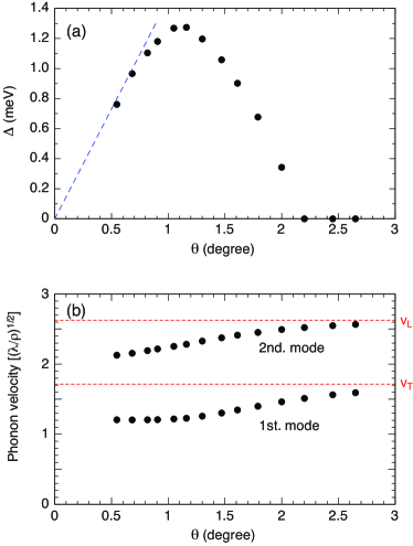
Importantly, we notice that the low-energy part of the phonon dispersion (scaled by $\omega_{0}$) is almost identical at $\theta=1.05^{\circ}$ and $0.547^{\circ}$ [Fig. 2(e) and (f)], indicating that it is converging to the universal structure in the low twist angle limit. This is somewhat surprising because the energy scale of the interlayer interacting potential $V_{0}$ (a constant) is increasing relative to the reference scale $\omega_{0}(\propto\theta)$ as $\theta$ decreases, so that one may naively expect the phonon band gap should increase relative to $\omega_{0}$ as well. In Fig. 5(a), we plot the width of the gap (in meV) between the second and the third branches as a function of the twist angle. In decreasing $\theta$, it takes the maximum around $\theta\sim 1.1^{\circ}$, and then it turns to decrease and approach the linear behavior in $\theta$, indicating the gap size in units of $\omega_{0}$ is converging to a constant value. Figure 5(b) shows the twist angle dependence of the phonon group velocities $\partial\omega/\partial q|_{q\to 0}$ for the first and the second $\mathbf{u}^{-}$ modes. In large twist angles, they become the velocities of the transverse ($v_{T}$) and longitudinal ($v_{L}$) acoustic phonon modes of single layer graphene (indicated by the horizontal dashed lines), as argued above. In decreasing the angle, the phonon velocities decrease as a result of the miniband formation, and they eventually approach constant values in the low angle limit.

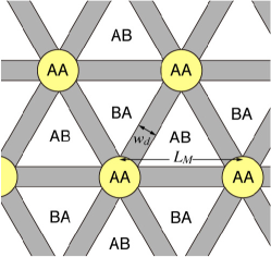
This universal feature of the scaled phonon dispersion can be understood by considering the domain-wall structure in the relaxed TBG, which is schematically illustrated as Fig. 6. Here triangular AB and BA regions are separated by the domain walls (gray regions) with AA stacked spots at vertices. It was shown that the characteristic width of the domain walls is almost independent of the twist angle Alden et al. (2013), and it is given by Nam and Koshino (2017)

$$w_{d}\approx\frac{a}{4}\sqrt{\frac{\lambda+\mu}{V_{0}}},$$ (23)

which is about 5 nm. The domain pattern becomes clear in low twist angles such that $L_{M}\gg w_{d}$, or $\theta$ lower than about 2 degrees. We first qualitatively understand the scale of $w_{d}$ by the following order estimation. The area of the domain wall per moiré unit cell is given by $\sim w_{d}L_{M}$ with the numerical factor neglected. The total interlayer binding energy (relative to the AB / BA stacking) per moiré unit cell is then $U_{B}\sim V_{0}(w_{d}L_{M})$. The elastic energy is also concentrated to the domain-wall regions and it is given by $U_{E}\sim\lambda(\partial u_{i}/\partial x_{j})^{2}(w_{d}L_{M})$. Here we took $\lambda$ as a representative scale for the elastic constant, since $\lambda$ and $\mu$ are in the same order of magnitude. In the domain wall, the strain tensor $\partial u_{i}/\partial x_{j}$ is of the order of $a/w_{d}$ since the atomic shift $u_{i}$ changes by about $a$ inside the domain wall. The relaxed state is given by the condition $U_{E}\sim U_{B}$, and this gives $w_{d}\sim a\sqrt{\lambda/V_{0}}$, which has the same order of magnitude as Eq. (23).

Now let us consider an oscillation of the moiré lattice around the relaxed state. We consider a simple excitation such as the Fig. 4(a) and (b), and assume the in-plane displacement of the AA positions (‘lattice points’) at $\mathbf{R}$ is $\tilde{\mathbf{u}}(\mathbf{R})$. During the oscillation, the binding energy and elastic energy are shown to be approximately proportional to the total length of the domain walls. In Figs. 4(a) and (b), we actually see that the domain walls (‘bonds’) are elongated (or shortened), and here the graphene’s atomic lattice is not stretched in the same direction, but the area of the same local atomic structure is just increased, so that the total energy change is proportional to the domain-wall length. The change of the total domain-wall length from the relaxed state is of the order of $\tilde{u}^{2}/L_{M}$ per a moiré unit cell, noting that the linear term in $\tilde{u}$ can be negative and positive place by place and vanishes in total. Therefore, the changes in the binding energy and the elastic energy are given by $\delta U_{B}\sim V_{0}w_{d}\,\tilde{u}^{2}/L_{M}$ and $\delta U_{E}\sim\lambda(a/w_{d})^{2}w_{d}\,\tilde{u}^{2}/L_{M}$, which are of the same order because $V_{0}\sim\lambda(a/w_{d})^{2}$ as argued above. The kinetic energy $T$ is estimated by considering the atomic motion. Here the change of the moiré lattice $\tilde{u}$ is actually caused by a change of the interlayer atomic shift $\mathbf{u}^{-}$ around the domain wall. Here we have a relation $\tilde{u}\sim(w_{d}/a)\delta u^{-}$, because a change of the atomic lattice of the order of $a$ is magnified to a change of moiré lattice by $w_{d}$. Considering that the atoms are oscillating only around the domain-wall regions, the kinetic energy per moiré unit cell is given by $T\sim\rho(\delta u^{-})^{2}\omega^{2}(w_{d}L_{M})=\rho(a/w_{d})^{2}\,\tilde{u}^{2}\omega^{2}(w_{d}L_{M})$ where $\omega$ is the oscillation frequency. By assuming the kinetic energy $T$ and the potential energy $U_{E}$ and $U_{B}$ are of the same order of magnitude, we end up with

$$\omega\sim\sqrt{\frac{\lambda}{\rho}}\frac{1}{L_{M}},$$ (24)

which correctly gives the order of $\omega_{0}$.

Based on the above argument, we can construct a simple effective model to describe the lowest two modes. We consider a triangular lattice composed of masses (corresponding to the AA spots) and bonds (domain walls) connecting the neighboring masses. We assume that the bonds are always straight and the energy of each bond is proportional to its length. We consider a vibration around the perfect triangular lattice with the lattice constant $L_{M}$, assuming that the total area of the system is fixed. If the in-plane displacement of the mass is given by $\tilde{\mathbf{u}}(\mathbf{R})$, the length change of the bonds summed over the whole system is given by

$$\Delta L_{\rm bond}=\sum_{\mathbf{R}}\sum_{i=1}^{3}\frac{1}{2L_{M}}\left[|\Delta\tilde{\mathbf{u}}^{(i)}(\mathbf{R})|^{2}-\Bigl{(}\Delta\tilde{\mathbf{u}}^{(i)}(\mathbf{R})\cdot\frac{\mathbf{L}^{M}_{i}}{L_{M}}\Bigr{)}^{2}\right]$$ (25)

where $\Delta\tilde{\mathbf{u}}^{(i)}(\mathbf{R})=\tilde{\mathbf{u}}(\mathbf{R}+\mathbf{L}^{M}_{i})-\tilde{\mathbf{u}}(\mathbf{R})$, the vector $\mathbf{R}=m\mathbf{L}^{M}_{1}+n\mathbf{L}^{M}_{2}$ runs over the lattice points, and we define $\mathbf{L}^{M}_{3}=\mathbf{L}^{M}_{2}-\mathbf{L}^{M}_{1}$. The total energy of the bonds is given by $\tilde{U}=\alpha V_{0}w_{d}\Delta L_{\rm bond}$, where $\alpha$ is a numerical factor of the order of 1 to match the energy scale with the original model. By the Fourier transformation $\tilde{\mathbf{u}}(\mathbf{R})=\sum_{\mathbf{q}}\tilde{\mathbf{u}}_{\mathbf{q}}e^{i\mathbf{q}\cdot\mathbf{R}}$, it is written as

$$\tilde{U}=\frac{1}{2}\sum_{\mathbf{q}}\tilde{\mathbf{u}}_{-\mathbf{q}}^{T}\hat{D}(\mathbf{q})\tilde{\mathbf{u}}_{\mathbf{q}},$$ (26)

where $\hat{D}(\mathbf{q})$ is the dynamical matrix defined by

$$D_{\mu\nu}(\mathbf{q})=\sum_{i=1}^{3}\frac{\alpha V_{0}w_{d}}{L_{M}}\Biggl{(}2\sin\frac{\mathbf{q}\cdot\mathbf{L}^{M}_{i}}{2}\Biggr{)}^{2}\Biggl{[}\delta_{\mu\nu}-\frac{(\mathbf{L}^{M}_{i})_{\mu}(\mathbf{L}^{M}_{i})_{\nu}}{L_{M}^{2}}\Biggr{]},$$ (27)

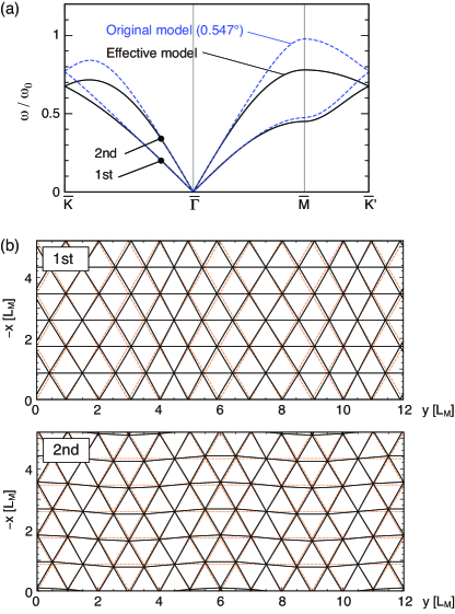
where $\mu,\nu=x,y$. The kinetic energy is given by $\tilde{T}=\frac{1}{2}\sum_{\mathbf{q}}M\dot{\tilde{\mathbf{u}}}_{-\mathbf{q}}\cdot\dot{\tilde{\mathbf{u}}}_{\mathbf{q}}$, where $M=\rho(a/w_{d})^{2}w_{d}L_{M}$ is the effective mass. Finally the equation of motion is given by $M\ddot{\tilde{\mathbf{u}}}_{\mathbf{q}}=-\hat{D}(\mathbf{q})\tilde{\mathbf{u}}_{\mathbf{q}}$. It is straight forward to see that the equation can be transformed to a dimensionless form by scaling the frequency by $\omega_{0}$. Figure 7(a) plots the phonon dispersion of this model, where the blue dashed line represents the original phonon dispersion of $\theta=0.547^{\circ}$. Here we choose $\alpha=2$ for the best fitting in the long wave-length region near $\bar{\Gamma}$. We see that the effective model qualitatively reproduces the whole dispersion relation of the original model for the first and second low-energy modes, and we can also show that the phonon wave functions are also correctly reproduced in the whole Brillouin zone. Figure 7(b) illustrates the wave functions of the first and the second modes at $\mathbf{q}=(0,2\pi/(6L_{M}))$, which agree with Figs. 4(a) and (b), respectively.

The vibration of the moiré lattice is different from that in an ordinary spring-mass model, in that the potential energy of a bond (a domain wall) is proportional to its length, but not to the squared length. This is directly related to the important property that the moiré longitudinal mode [Fig. 4(a)] has a lower frequency than the moiré transverse mode [Fig. 4(b)] unlike in the usual elastic system. In the ordinary spring-mass model, the strain energy of the moiré longitudinal mode as in Fig. 4(a) is mostly contributed from the bonds parallel to the wave vector (horizontal bonds in this figure), where the length change gives the tensile energy cost. In the present system, however, the horizontal bonds do not change the total energy because elongated bonds and shortened bonds just cancel in the total length, while the diagonal bonds contribute to a relatively small increase in the total length. In the effective lattice model given by Eq. (27), it is straight forward to check that the phonon frequency of the transverse mode is $\sqrt{3}$ times as large as that of the longitudinal mode in the long wave-length limit. In the original model, the ratio of the second band frequency to the first is about 1.8 near the $\Gamma$ point, indicating that the effective model is valid.

The linear dependence of energy for elongation of bonds implies that there is a constant force for all stretching modes, while such modes are prohibited in the present calculation because the moiré unit cell size $L_{M}$ is fixed. In the original lattice model for TBG, the all stretching mode corresponds to the overall interlayer rotation to reduce the twist angle $\theta$, where the moiré unit cell monotonically expands. The total energy (per area) then decreases because the area of the AB regions increases in proportion to $L_{M}^{2}$, and it eventually dominates over the area of the domain walls (with the width fixed to $w_{d}$), which is just in proportion to $L_{M}$. In experiments, a TBG with a finite twist angle can also exist as a meta-stable phase, where certain external constraints caused by local pinning mechanisms should prohibit the global rotation. The calculation fixing moiré unit cell size should be justified in such a situation.

As a final remark, we notice that the third lowest phonon band in Fig. 2 becomes flatter when the twist angle is reduced, resulting in a significant enhancement of phonon density of states as $\theta$ decreases. The corresponding wave function in Fig. 4(c) can be viewed as a ‘domain-breathing’ mode where triangular AB and BA domains expand and shrink in opposite phases. One may also view this mode as an in-plane optical mode of the moiré lattice. Here we see that the positions of the corner points of triangles are fixed during the oscillation. This means that the oscillation of a triangle does not affect that of neighboring triangles, so the system can be approximately viewed as independent oscillators. We presume that it is the reason for the flat band nature, i.e. the constant frequency independent of the wave number. The fourth and the fifth modes [Fig. 4(d) and (e)] exhibit complicated wave patterns including the bending of the domain walls and also the distortion of AA spots.

IV Considerations on the flexural phonon

While the current model only considered the in-plane phonons, the actual TBG also has the flexural phonon modes vibrating in the out-of-plane direction. Here we consider the effect of moiré interlayer coupling on the flexural phonons in TBG by the following simple qualitative argument. We consider three-dimenisional displacement $\mathbf{u}^{(l)}=(u_{x}^{(l)},u_{y}^{(l)},u_{z}^{(l)})$ from the nondistorted configuration in which two flat graphenes are stacked with interlayer spacing $d_{AB}$ (the distance for the AB-stacked bilayer). It is known that the relaxed TBG is corrugated in such a way that the spacing is minimum at AB/BA-stacking regions and maximum at AA-stacking regions Uchida et al. (2014); van Wijk et al. (2015); Lin et al. (2018). We can define the optimized interlayer spacing $d_{\rm opt}(\mbox{\boldmath$\delta$})$ as a function of the two-dimensional sliding vector $\mbox{\boldmath$\delta$}(\mathbf{r})$ [Eq. (5)]. The interlayer binding potential for the vertical displacement $(u^{(1)}_{z},u^{(2)}_{z})$ can then be written as a quadratic form $V_{\perp}=\alpha[u^{-}_{z}+d_{AB}-d_{\rm opt}(\mbox{\boldmath$\delta$})]^{2}$, where $u^{-}_{z}=u^{(2)}_{z}-u^{(1)}_{z}$. The total binding energy is a sum of $V_{\perp}$ and the in-plane part, Eq. (7). The potential curvature $\alpha$ is shown to be nearly independent of the stacking structure, Lee et al. (2008) so we assume $\alpha$ is constant. The effect of the moiré superlattice comes only from the potential term through $\mbox{\boldmath$\delta$}=\mbox{\boldmath$\delta$}(\mathbf{r})$. The kinetic part and elastic part are unchanged from the intrinsic graphene’s and do not depend on $\delta$. In the equation of motion, we have the force term $\partial V_{\perp}/\partial u_{z}=2\alpha[u^{-}_{z}+d_{AB}-d_{\rm opt}(\mbox{\boldmath$\delta$})]$, and the optimized corrugated structure is given by $u^{-}_{0z}=d_{\rm opt}(\mbox{\boldmath$\delta$})-d_{AB}$. When we consider an excitation from the optimized state $\mathbf{u}^{-}=\mathbf{u}^{-}_{0}+\delta\mathbf{u}^{-}$, the force term becomes $\partial V_{\perp}/\partial u_{z}=2\alpha\delta u^{-}_{z}$, and does not depend on $\delta$ anymore, i.e., the superlattice effect vanishes in the equation of motion for $\delta u^{-}_{z}$.

From these arguments, we presume that the flexural phonon does not exhibit well-pronounced miniband structure unlike the in-plane asymmetric modes, and the corresponding phonon density of states remains mostly unchanged from the intrinsic graphene. Actually the minigap formation was not observed in a phonon calculation fully including all the atomic sites in TBG with the registry-dependent interlayer interaction Choi and Choi (2018); Angeli et al. (2019). It implies that the flexural phonons remain almost intact, considering that the density of states in the low-energy region of graphene is dominated by the flexural phonons Lindsay et al. (2010). Rigorously speaking, the corrugated structure should cause some finite coupling between the in-plane modes and out-of-plane modes, and we leave the detailed study of the full three-dimensional phonon problem for future works.

V Conclusion

We studied the in-plane acoustic phonons of low-angle TBGs using the continuum approach. We found that the moiré superlattice effect only affects the in-plane asymmetric modes where the linear dispersion of the acoustic phonon is reconstructed into minibands separated by gaps, while the in-plane symmetric modes remain intact. The phonon wave functions for in-plane asymmetric modes can be regarded as vibrations of the triangular superlattice, and they are qualitatively understood by the effective lattice model of the moiré scale.

Our calculation shows that 50% of the linear acoustic modes of the TBG are completely reconstructed by the moiré superlattice coupling and their phonon velocities are significantly lowered. Moreover, it is also shown that as the twist angle decreases, the characteristic flat phonon mode with diverging density of states is generated. We expect that these effects should affect the thermal conductivity directly and also phonon-related thermal phenomena. The electron-phonon coupling between the flat-band electrons and the moiré phonons, and its effect on the superconducting and correlating states, are also important problems. We leave these issues for future study.

VI Acknowledgments

M. K. acknowledges fruitful discussions with Pablo Jarillo-Herrero, Philip Kim and Debanjan Chowdhury. M. K. acknowledges the financial support of JSPS KAKENHI Grant Number JP17K05496. Y.-W.S. was supported by National Research Foundation of Korea (Grant No. 2017R1A5A1014862, SRC program: vdWMRC center).

References

- Berger et al. (2006) Claire Berger, Zhimin Song, Xuebin Li, Xiaosong Wu, Nate Brown, Cécile Naud, Didier Mayou, Tianbo Li, Joanna Hass, Alexei N. Marchenkov, Edward H. Conrad, Phillip N. First, and Walt A. de Heer, “Electronic confinement and coherence in patterned epitaxial graphene,” Science 312, 1191–1196 (2006).
- Hass et al. (2007) J. Hass, R. Feng, JE Millan-Otoya, X. Li, M. Sprinkle, PN First, WA De Heer, EH Conrad, and C. Berger, “Structural properties of the multilayer graphene/4H-SiC (000) system as determined by surface X-ray diffraction,” Phys. Rev. B 75, 214109 (2007).
- Hass et al. (2008) J. Hass, F. Varchon, J.E. Millan-Otoya, M. Sprinkle, N. Sharma, W.A. de Heer, C. Berger, P.N. First, L. Magaud, and E.H. Conrad, “Why multilayer graphene on 4H-SiC (000) behaves like a single sheet of graphene,” Phys. Rev. Lett. 100, 125504 (2008).
- Li et al. (2009) G. Li, A. Luican, J. M. B. Lopes dos Santos, A.H.C. Neto, A. Reina, J. Kong, and EY Andrei, “Observation of van hove singularities in twisted graphene layers,” Nature Physics 6, 109–113 (2009).
- Miller et al. (2010) D.L. Miller, K.D. Kubista, G.M. Rutter, M. Ruan, W.A. de Heer, P.N. First, and J.A. Stroscio, “Structural analysis of multilayer graphene via atomic moiré interferometry,” Phys. Rev. B 81, 125427 (2010).
- Luican et al. (2011) A. Luican, G. Li, A. Reina, J. Kong, RR Nair, KS Novoselov, AK Geim, and EY Andrei, “Single-layer behavior and its breakdown in twisted graphene layers,” Phys. Rev. Lett. 106, 126802 (2011).
- Lopes dos Santos et al. (2007) JMB Lopes dos Santos, NMR Peres, and AH Castro Neto, “Graphene bilayer with a twist: Electronic structure,” Phys. Rev. Lett. 99, 256802 (2007).
- Mele (2010) E.J. Mele, “Commensuration and interlayer coherence in twisted bilayer graphene,” Phys. Rev. B 81, 161405 (2010).
- Trambly de Laissardière et al. (2010) G. Trambly de Laissardière, D. Mayou, and L. Magaud, “Localization of dirac electrons in rotated graphene bilayers,” Nano Lett. 10, 804–808 (2010).
- Shallcross et al. (2010) S. Shallcross, S. Sharma, E. Kandelaki, and OA Pankratov, “Electronic structure of turbostratic graphene,” Phys. Rev. B 81, 165105 (2010).
- Morell et al. (2010) E.S. Morell, JD Correa, P. Vargas, M. Pacheco, and Z. Barticevic, “Flat bands in slightly twisted bilayer graphene: Tight-binding calculations,” Phys. Rev. B 82, 121407 (2010).
- Bistritzer and MacDonald (2011) R. Bistritzer and A.H. MacDonald, “Moiré bands in twisted double-layer graphene,” Proc. Natl. Acad. Sci. 108, 12233 (2011).
- Kindermann and First (2011) M. Kindermann and PN First, “Local sublattice-symmetry breaking in rotationally faulted multilayer graphene,” Phys. Rev. B 83, 045425 (2011).
- Xian et al. (2011) L. Xian, S. Barraza-Lopez, and MY Chou, “Effects of electrostatic fields and charge doping on the linear bands in twisted graphene bilayers,” Phys. Rev. B 84, 075425 (2011).
- Lopes dos Santos et al. (2012) J. M. B. Lopes dos Santos, N. M. R. Peres, and A. H. Castro Neto, “Continuum model of the twisted graphene bilayer,” Phys. Rev. B 86, 155449 (2012).
- Moon and Koshino (2012) Pilkyung Moon and Mikito Koshino, “Energy spectrum and quantum hall effect in twisted bilayer graphene,” Phys. Rev. B 85, 195458 (2012).
- de Laissardiere et al. (2012) G Trambly de Laissardiere, D Mayou, and L Magaud, “Numerical studies of confined states in rotated bilayers of graphene,” Phys. Rev. B 86, 125413 (2012).
- Moon and Koshino (2013) Pilkyung Moon and Mikito Koshino, “Optical absorption in twisted bilayer graphene,” Phys. Rev. B 87, 205404 (2013).
- Weckbecker et al. (2016) D. Weckbecker, S. Shallcross, M. Fleischmann, N. Ray, S. Sharma, and O. Pankratov, “Low-energy theory for the graphene twist bilayer,” Phys. Rev. B 93, 035452 (2016).
- Cao et al. (2018a) Yuan Cao, Valla Fatemi, Shiang Fang, Kenji Watanabe, Takashi Taniguchi, Efthimios Kaxiras, and Pablo Jarillo-Herrero, “Unconventional superconductivity in magic-angle graphene superlattices,” Nature 556, 43 (2018a).
- Cao et al. (2018b) Yuan Cao, Valla Fatemi, Ahmet Demir, Shiang Fang, Spencer L. Tomarken, Jason Y. Luo, Javier D. Sanchez-Yamagishi, Kenji Watanabe, Takashi Taniguchi, Efthimios Kaxiras, Ray C. Ashoori, and Pablo Jarillo-Herrero, “Correlated insulator behaviour at half-filling in magic-angle graphene superlattices,” Nature 556, 80 (2018b).
- Yankowitz et al. (2019) Matthew Yankowitz, Shaowen Chen, Hryhoriy Polshyn, Yuxuan Zhang, K Watanabe, T Taniguchi, David Graf, Andrea F Young, and Cory R Dean, “Tuning superconductivity in twisted bilayer graphene,” Science 363, 1059 (2019).
- Popov et al. (2011) Andrey M Popov, Irina V Lebedeva, Andrey A Knizhnik, Yurii E Lozovik, and Boris V Potapkin, “Commensurate-incommensurate phase transition in bilayer graphene,” Phys. Rev. B 84, 045404 (2011).
- Brown et al. (2012) Lola Brown, Robert Hovden, Pinshane Huang, Michal Wojcik, David A Muller, and Jiwoong Park, “Twinning and twisting of tri-and bilayer graphene,” Nano letters 12, 1609–1615 (2012).
- Lin et al. (2013) Junhao Lin, Wenjing Fang, Wu Zhou, Andrew R Lupini, Juan Carlos Idrobo, Jing Kong, Stephen J Pennycook, and Sokrates T Pantelides, “Ac/ab stacking boundaries in bilayer graphene,” Nano Lett. 13, 3262–3268 (2013).
- Alden et al. (2013) Jonathan S. Alden, Adam W. Tsen, Pinshane Y. Huang, Robert Hovden, Lola Brown, Jiwoong Park, David A. Muller, and Paul L. McEuen, “Strain solitons and topological defects in bilayer graphene,” PNAS 110, 11256–11260 (2013).
- van Wijk et al. (2015) MM van Wijk, A Schuring, MI Katsnelson, and A Fasolino, “Relaxation of moiré patterns for slightly misaligned identical lattices: graphene on graphite,” 2D Mater. 2, 034010 (2015).
- Dai et al. (2016) Shuyang Dai, Yang Xiang, and David J Srolovitz, “Twisted bilayer graphene: Moiré with a twist,” Nano letters 16, 5923–5927 (2016).
- Jain et al. (2016) Sandeep K Jain, Vladimir Juričić, and Gerard T Barkema, “Structure of twisted and buckled bilayer graphene,” 2D Mater. 4, 015018 (2016).
- Nam and Koshino (2017) Nguyen N. T. Nam and Mikito Koshino, “Lattice relaxation and energy band modulation in twisted bilayer graphene,” Phys. Rev. B 96, 075311 (2017).
- Carr et al. (2018) Stephen Carr, Daniel Massatt, Steven B. Torrisi, Paul Cazeaux, Mitchell Luskin, and Efthimios Kaxiras, “Relaxation and domain formation in incommensurate two-dimensional heterostructures,” Phys. Rev. B 98, 224102 (2018).
- Lin et al. (2018) Xianqing Lin, Dan Liu, and David Tománek, “Shear instability in twisted bilayer graphene,” Phys. Rev. B 98, 195432 (2018).
- Yoo et al. (2019) Hyobin Yoo, Rebecca Engelke, Stephen Carr, Shiang Fang, Kuan Zhang, Paul Cazeaux, Suk Hyun Sung, Robert Hovden, Adam W Tsen, Takashi Taniguchi, Gyu-Chul Watanabe, Kenji Yi, Miyoung Kim, Luskin Mitchell, Ellad B. Tadmor, Efthimios Kaxiras, and Philip Kim, “Atomic and electronic reconstruction at the van der waals interface in twisted bilayer graphene,” Nature materials 18, 448 (2019).
- Walet and Guinea (2019) Niels R Walet and Francisco Guinea, “Lattice deformation, low energy models and flat bands in twisted graphene bilayers,” arXiv preprint arXiv:1903.00340 (2019).
- Uchida et al. (2014) Kazuyuki Uchida, Shinnosuke Furuya, Jun-Ichi Iwata, and Atsushi Oshiyama, “Atomic corrugation and electron localization due to moiré patterns in twisted bilayer graphenes,” Phys. Rev. B 90, 155451 (2014).
- Koshino et al. (2018) Mikito Koshino, Noah FQ Yuan, Takashi Koretsune, Masayuki Ochi, Kazuhiko Kuroki, and Liang Fu, “Maximally localized wannier orbitals and the extended hubbard model for twisted bilayer graphene,” Phys. Rev. X 8, 031087 (2018).
- Lucignano et al. (2019) Procolo Lucignano, Dario Alfè, Vittorio Cataudella, Domenico Ninno, and Giovanni Cantele, “Crucial role of atomic corrugation on the flat bands and energy gaps of twisted bilayer graphene at the magic angle ,” Phys. Rev. B 99, 195419 (2019).
- Woods et al. (2014) CR Woods, L Britnell, A Eckmann, RS Ma, JC Lu, HM Guo, X Lin, GL Yu, Y Cao, RV Gorbachev, et al., “Commensurate-incommensurate transition in graphene on hexagonal boron nitride,” Nature physics 10, 451–456 (2014).
- San-Jose et al. (2014a) Pablo San-Jose, A Gutiérrez-Rubio, Mauricio Sturla, and Francisco Guinea, “Spontaneous strains and gap in graphene on boron nitride,” Phys. Rev. B 90, 075428 (2014a).
- San-Jose et al. (2014b) Pablo San-Jose, A Gutiérrez-Rubio, Mauricio Sturla, and Francisco Guinea, “Electronic structure of spontaneously strained graphene on hexagonal boron nitride,” Physical Review B 90, 115152 (2014b).
- Jung et al. (2015) Jeil Jung, Ashley M DaSilva, Allan H MacDonald, and Shaffique Adam, “Origin of band gaps in graphene on hexagonal boron nitride,” Nature communications 6, 6308 (2015).
- Grüneis et al. (2002) A Grüneis, R Saito, T Kimura, LG Cançado, MA Pimenta, A Jorio, AG Souza Filho, G Dresselhaus, and MS Dresselhaus, “Determination of two-dimensional phonon dispersion relation of graphite by raman spectroscopy,” Physical review B 65, 155405 (2002).
- Suzuura and Ando (2002) Hidekatsu Suzuura and Tsuneya Ando, “Phonons and electron-phonon scattering in carbon nanotubes,” Physical review B 65, 235412 (2002).
- Yan et al. (2008) Jia-An Yan, WY Ruan, and MY Chou, “Phonon dispersions and vibrational properties of monolayer, bilayer, and trilayer graphene: Density-functional perturbation theory,” Physical review B 77, 125401 (2008).
- Nika and Balandin (2017) Denis L Nika and Alexander A Balandin, “Phonons and thermal transport in graphene and graphene-based materials,” Reports on Progress in Physics 80, 036502 (2017).
- Jiang et al. (2012) Jin-Wu Jiang, Bing-Shen Wang, and Timon Rabczuk, “Acoustic and breathing phonon modes in bilayer graphene with moiré patterns,” Applied Physics Letters 101, 023113 (2012).
- Cocemasov et al. (2013) Alexandr I Cocemasov, Denis L Nika, and Alexander A Balandin, “Phonons in twisted bilayer graphene,” Physical Review B 88, 035428 (2013).
- Choi and Choi (2018) Young Woo Choi and Hyoung Joon Choi, “Strong electron-phonon coupling, electron-hole asymmetry, and nonadiabaticity in magic-angle twisted bilayer graphene,” Physical Review B 98, 241412 (2018).
- Angeli et al. (2019) M Angeli, E Tosatti, and M Fabrizio, “Valley Jahn-teller effect in twisted bilayer graphene,” arXiv preprint arXiv:1904.06301 (2019).
- Felix and Pereira (2018) Isaac M Felix and Luiz Felipe C Pereira, “Thermal conductivity of graphene-hbn superlattice ribbons,” Scientific reports 8, 2737 (2018).
- Wu et al. (2018) Fengcheng Wu, AH MacDonald, and Ivar Martin, “Theory of phonon-mediated superconductivity in twisted bilayer graphene,” Phys. Rev. Lett. 121, 257001 (2018).
- Wu et al. (2019) Fengcheng Wu, Euyheon Hwang, and Sankar Das Sarma, “Phonon-induced giant linear-in- resistivity in magic angle twisted bilayer graphene: Ordinary strangeness and exotic superconductivity,” Phys. Rev. B 99, 165112 (2019).
- Lebedeva et al. (2011) Irina V Lebedeva, Andrey A Knizhnik, Andrey M Popov, Yurii E Lozovik, and Boris V Potapkin, “Interlayer interaction and relative vibrations of bilayer graphene,” Physical Chemistry Chemical Physics 13, 5687–5695 (2011).
- Zakharchenko et al. (2009) KV Zakharchenko, MI Katsnelson, and Annalisa Fasolino, “Finite temperature lattice properties of graphene beyond the quasiharmonic approximation,” Physical review letters 102, 046808 (2009).
- Lee et al. (2008) Jae-Kap Lee, Seung-Cheol Lee, Jae-Pyoung Ahn, Soo-Chul Kim, John IB Wilson, and Phillip John, “The growth of aa graphite on (111) diamond,” The Journal of chemical physics 129, 234709 (2008).
- Lindsay et al. (2010) L Lindsay, DA Broido, and Natalio Mingo, “Flexural phonons and thermal transport in graphene,” Physical Review B 82, 115427 (2010).