Flexible Computational Pipelines for Robust Abstraction-Based Control Synthesis

Abstract

Successfully synthesizing controllers for complex dynamical systems and specifications often requires leveraging domain knowledge as well as making difficult computational or mathematical tradeoffs. This paper presents a flexible and extensible framework for constructing robust control synthesis algorithms and applies this to the traditional abstraction-based control synthesis pipeline. It is grounded in the theory of relational interfaces and provides a principled methodology to seamlessly combine different techniques (such as dynamic precision grids, refining abstractions while synthesizing, or decomposed control predecessors) or create custom procedures to exploit an application’s intrinsic structural properties. A Dubins vehicle is used as a motivating example to showcase memory and runtime improvements.

1 Introduction

A control synthesizer’s high level goal is to automatically construct control software that enables a closed loop system to satisfy a desired specification. A vast and rich literature contains results that mathematically characterize solutions to different classes of problems and specifications, such as the Hamilton-Jacobi-Isaacs PDE for differential games [2], Lyapunov theory for stabilization [8], and fixed-points for temporal logic specifications [17][11]. While many control synthesis problems have elegant mathematical solutions, there is often a gap between a solution’s theoretical characterization and the algorithms used to compute it. What data structures are used to represent the dynamics and constraints? What operations should those data structures support? How should the control synthesis algorithm be structured? Implementing solutions to the questions above can require substantial time. This problem is especially critical for computationally challenging problems, where it is often necessary to let the user rapidly identify and exploit structure through analysis or experimentation.

1.1 Bottlenecks in Abstraction-based Control Synthesis

This paper’s goal is to enable a framework to develop extensible tools for robust controller synthesis. It was inspired in part by computational bottlenecks encountered in control synthesizers that construct finite abstractions of continuous systems, which we use as a target use case. A traditional abstraction-based control synthesis pipeline consists of three distinct stages:

1. Abstracting the continuous state system into a finite automaton whose underlying transitions faithfully mimic the original dynamics [21], [23].

2. Synthesizing a discrete controller by leveraging data structures and symbolic reasoning algorithms to mitigate combinatorial state explosion.

3. Refining the discrete controller into a continuous one. Feasibility of this step is ensured through the abstraction step.

This pipeline appears in tools PESSOA [12] and SCOTS [19], which can exhibit acute computational bottlenecks for high dimensional and nonlinear system dynamics. A common method to mitigate these bottlenecks is to exploit a specific dynamical system’s topological and algebraic properties. In MASCOT [7] and CoSyMA [14], multi-scale grids and hierarchical models capture notions of state-space locality. One could incrementally construct an abstraction of the system dynamics while performing the control synthesis step [15] [10] as implemented in tools ROCS [9] and ARCS [4]. The abstraction overhead can also be reduced by representing systems as a collection of components composed in parallel [13] [6]. These have been developed in isolation and were not previously interoperable.

1.2 Methodology

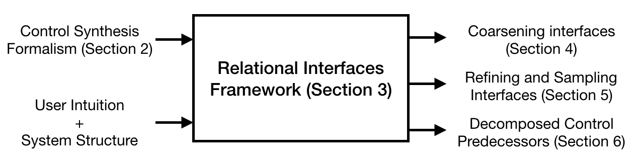
Figure 1: By expressing many different techniques within a common framework, users are able to rapidly develop methods to exploit system structure in controller synthesis.

Figure 1 depicts this paper’s methodology and organization. The existing control synthesis formalism does not readily lend itself to algorithmic modifications that reflect and exploit structural properties in the system and specification. We use the theory of relational interfaces [22] as a foundation and augment it to express control synthesis pipelines. Interfaces are used to represent both system models and constraints. A small collection of atomic operators manipulates interfaces and is powerful enough to reconstruct many existing control synthesis pipelines.

One may also add new composite operators to encode desirable heuristics that exploit structural properties in the system and specifications. The last three sections encode the techniques for abstraction-based control synthesis from Section 1.1 within the relational interfaces framework. By deliberately deconstructing those techniques, then reconstructing them within a compositional framework it was possible to identify implicit or unnecessary assumptions then generalize or remove them. It also makes the aforementioned techniques interoperable amongst themselves as well as future techniques.

Interfaces come equipped with a refinement partial order that formalizes when one interface abstracts another. This paper focuses on preserving the refinement relation and sufficient conditions to refine discrete controllers back to concrete ones. Additional guarantees regarding completeness, termination, precision, or decomposability can be encoded, but impose additional requirements on the control synthesis algorithm and are beyond the scope of this paper.

1.3 Contributions

To our knowledge, the application of relational interfaces to robust abstraction-based control synthesis is new. The framework’s building blocks consist of a collection of small, well understood operators that are nonetheless powerful enough to express many prior techniques. Encoding these techniques as relational interface operations forced us to simplify, formalize, or remove implicit assumptions in existing tools. The framework also exhibits numerous desirable features.

1. It enables compositional tools for control synthesis by leveraging a theoretical foundation with compositionality built into it. This paper showcases a principled methodology to seamlessly combine the methods in Section 1.1, as well as construct new techniques.

2. It enables a declarative approach to control synthesis by enforcing a strict separation between the high level algorithm from its low level implementation. We rely on the availability of an underlying data structure to encode and manipulate predicates. Low level predicate operations, while powerful, make it easy to inadvertently violate the refinement property. Conforming to the relational interface operations minimizes this danger.

This paper’s first half is domain agnostic and applicable to general robust control synthesis problems. The second half applies those insights to the finite abstraction approach to control synthesis. A smaller Dubins vehicle example is used to showcase and evaluate different techniques and their computational gains, compared to the unoptimized problem. A 6D lunar lander example is included in the appendix which leverages all of the techniques in this paper collectively.

1.4 Notation

Let $=$ be an assertion that two objects are mathematically equivalent; as a special case ‘$\equiv$’ is used when those two objects are sets. In contrast, the operator ‘$==$’ checks whether two objects are equivalent, returning true if they are and false otherwise. A special instance of ‘$==$’ is logical equivalence ‘$\Leftrightarrow$’.

Variables are denoted by lower case letters. Each variable $v$ is associated with a domain of values $\mathcal{D}(v)$ that is analogous to the variable’s type. A composite variable is a set of variables and is analogous to a bundle of wrapped wires. From a collection of variables $v_{1},\ldots,v_{M}$ a composite variable $v$ can be constructed by taking the union $v\equiv v_{1}\cup\ldots\cup v_{M}$ and the domain $\mathcal{D}(v)\equiv\prod_{i=1}^{M}\mathcal{D}(v_{i})$. Note that the variables $v_{1},\ldots,v_{M}$ above may themselves be composite. As an example if $v$ is associated with a $M$-dimensional Euclidean space $\mathbb{R}^{M}$, then it is a composite variable that can be broken apart into a collection of atomic variables $v_{1},\ldots,v_{M}$ where $\mathcal{D}(v_{i})\equiv\mathbb{R}$ for all $i\in\{1,\ldots,M\}$. The technical results herein do not distinguish between composite and atomic variables.

Predicates are functions that map variable assignments to a Boolean value. Predicates that stand in for expressions/formulas are denoted with capital letters. Predicates $P$ and $Q$ are logically equivalent (denoted by $P\Leftrightarrow Q$) if and only if $P\Rightarrow Q$ and $Q\Rightarrow P$ are true for all variable assignments. The universal and existential quantifiers $\forall$ and $\exists$ eliminate variables and yield new predicates. Predicates ${\exists w}P$ and ${\forall w}P$ do not depend on $w$. If $w$ is a composite variable $w\equiv w_{1}\cup\ldots\cup w_{N}$ then ${\exists w}P$ is simply a shorthand for ${\exists w_{1}}\ldots{\exists w_{N}}P$.

2 Control Synthesis for a Motivating Example

As a simple, instructive example consider a planar Dubins vehicle that is tasked with reaching a desired location. Let $x=\{p_{x},p_{y},\theta\}$ be the collection of state variables, $u=\{v,\omega\}$ be a collection input variables to be controlled, $x^{+}=\{p_{x}^{+},p_{y}^{+},\theta^{+}\}$ represent state variables at a subsequent time step, and $L=1.4$ be a constant representing the vehicle length. The constraints

$$p_{x}^{+} ==p_{x}+v\cos(\theta) F_{x}$$ ()

$$p_{y}^{+} ==p_{y}+v\sin(\theta) F_{y}$$ ()

$$\theta^{+} ==\theta+\dfrac{v}{L}\sin(\omega) F_{\theta}$$ ()

characterize the discrete time dynamics. The continuous state domain is $\mathcal{D}(x)\equiv[-2,2]\times[-2,2]\times[-\pi,\pi)$, where the last component is periodic so $-\pi$ and $\pi$ are identical values. The input domains are $\mathcal{D}(v)\equiv\{0.25,0.5\}$ and $\mathcal{D}(\omega)\equiv\{-1.5,0,1.5\}$

Let predicate $F=F_{x}\and F_{y}\and F_{\theta}$ represent the monolithic system dynamics. Predicate $T$ depends only on $x$ and represents the target set $[-0.4,0.4]\times[-0.4,0.4]\times[-\pi,\pi)$, encoding that the vehicle’s position must reach a square with any orientation. Let $Z$ be a predicate that depends on variable $x^{+}$ that encodes a collection of states at a future time step. Equation 1 characterizes the robust controlled predecessor, which takes $Z$ and computes the set of states from which there exists a non-blocking assignment to $u$ that guarantees $x^{+}$ will satisfy $Z$, despite any non-determinism contained in $F$. The term ${\exists x^{+}}F$ prevents state-control pairs from blocking, while ${\forall x^{+}}(F\Rightarrow Z)$ encodes the state-control pairs that guarantee satisfaction of $Z$.

$${\text{{cpre}}}(F,Z)={\exists u}({\exists x^{+}}F\and{\forall x^{+}}(F\Rightarrow Z)).$$ (1)

The controlled predecessor is used to solve safety and reach games. We can solve for a region for which the target $T$ (respectively, safe set $S$) can be reached (made invariant) via an iteration of an appropriate reach (safe) operator. Both iterations are given by:

$$\text{Reach Iter:}\qquad Z_{0} =\bot\qquad Z_{i+1}=\text{{reach}}(F,Z_{i},T)={\text{{cpre}}}(F,Z_{i})\vee T.$$ (2)

$$\text{Safety Iter:}\qquad Z_{0} =S\qquad Z_{i+1}=\text{{safe}}(F,Z_{i},S)={\text{{cpre}}}(F,Z_{i})\and S.$$ (3)

The above iterations are not guaranteed to reach a fixed point in a finite number of iterations, except under certain technical conditions [21].

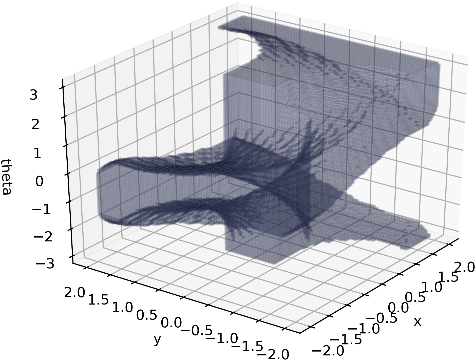
Figure 2: Approximate solution to the Dubins vehicle reach game visualized as a subset of the state space.

Figure 2 depicts an approximate region where the controller can force the Dubins vehicle to enter $T$. We showcase different improvements relative to a base line script used to generate Figure 2. A toolbox that adopts this paper’s framework is being actively developed and is open sourced at [1]. It is written in python 3.6 and uses the dd package as an interface to CUDD[20], a library in C/C++ for constructing and manipulating binary decision diagrams (BDD). All experiments were run on a single core of a 2013 Macbook Pro with 2.4GHz Intel Core i7 and 8GB of RAM.

The following section uses relational interfaces to represent the controlled predecessor ${\text{{cpre}}}(\cdot)$ and iterations (2) and (3) as a computational pipeline. Subsequent sections show how modifying this pipeline leads to favorable theoretical properties and computational gains.

3 Relational Interfaces

Relational interfaces are predicates augmented with annotations about each variable’s role as an input or output . They abstract away a component’s internal implementation and only encode an input-output relation.

Definition 1 (Relational Interface [22])

An interface $M(i,o)$ consists of a predicate $M$ over a set of input variables $i$ and output variables $o$.

For an interface $M(i,o)$, we call $(i,o)$ its input-output signature. An interface is a sink if it contains no outputs and has signature like $(i,{\varnothing})$, and a source if it contains no inputs like $({\varnothing},o)$. Sinks and source interfaces can be interpreted as sets whereas input-output interfaces are relations. Interfaces encode relations through their predicates and can capture features such as non-deterministic outputs or blocking (i.e., disallowed, error) inputs. A system blocks for an input assignment if there does not exist a corresponding output assignment that satisfies the interface relation. Blocking is a critical property used to declare requirements; sink interfaces impose constraints by modeling constrain violations as blocking inputs. Outputs on the other hand exhibit non-determinism, which is treated as an adversary. When one interface’s outputs are connected to another’s inputs, the outputs seek to cause blocking whenever possible.

3.1 Atomic and Composite Operators

Operators are used to manipulate interfaces by taking interfaces and variables as inputs and yielding another interface. We will show how the controlled predecessor ${\text{{cpre}}}(\cdot)$ in (1) can be constructed by composing operators appearing in [22] and one additional one. The first, output hiding, removes interface outputs.

Definition 2 (Output Hiding [22])

Output hiding operator $\text{{ohide}}(w,F)$ over interface $F(i,o)$ and outputs $w$ yields an interface with signature $(i,o\setminus w)$.

$$\text{{ohide}}(w,F)={\exists w}F$$ (4)

Existentially quantifying out $w$ ensures that the input-output behavior over the unhidden variables is still consistent with potential assignments to $w$. The operator $\text{{nb}}(\cdot)$ is a special variant of $\text{{ohide}}(\cdot)$ that hides all outputs, yielding a sink encoding all non-blocking inputs to the original interface.

Definition 3 (Nonblocking Inputs Sink)

Given an interface $F(i,o)$, the nonblocking operation nb(F) yields a sink interface with signature $(i,{\varnothing})$ and predicate $\text{{nb}}(F)={\exists o}F$. If $F(i,{\varnothing})$ is a sink interface, then $\text{{nb}}(F)=F$ yields itself. If $F({\varnothing},o)$ is a source interface, then $\text{{nb}}(F)=\bot$ if and only if $F\Leftrightarrow\bot$; otherwise $\text{{nb}}(F)=\top$.

The interface composition operator takes multiple interfaces and “collapses” them into a single input-output interface. It can be viewed as a generalization of function composition in the special case where each interface encodes a total function (i.e., deterministic output and inputs never block).

Definition 4 (Interface Composition [22])

Let $F_{1}(i_{1},o_{1})$ and $F_{2}(i_{2},o_{2})$ be interfaces with disjoint output variables $o_{1}\cap o_{2}\equiv{\varnothing}$ and $i_{1}\cap o_{2}\equiv{\varnothing}$ which signifies that $F_{2}$’s outputs may not be fed back into $F_{1}$’s inputs. Define new composite variables

$$io_{12} \equiv o_{1}\cap i_{2}$$ (5)

$$i_{12} \equiv(i_{1}\cup i_{2})\setminus io_{12}$$ (6)

$$o_{12} \equiv o_{1}\cup o_{2}.$$ (7)

Composition $\text{{comp}}(F_{1},F_{2})$ is an interface with signature $(i_{12},o_{12})$ and predicate

$$F_{1}\and F_{2}\and{\forall o_{12}}(F_{1}\Rightarrow\text{{nb}}(F_{2})).$$ (8)

Interface subscripts may be swapped if instead $F_{2}$’s outputs are fed into $F_{1}$.

Interfaces $F_{1}$ and $F_{2}$ are composed in parallel if $io_{21}\equiv{\varnothing}$ holds in addition to $io_{12}\equiv{\varnothing}$. Equation 8 under parallel composition reduces to $F_{1}\and F_{2}$ (Lemma 6.4 in [22]) and $\text{{comp}}(\cdot)$ is commutative and associative. If $io_{12}\not\equiv{\varnothing}$, then they are composed in series and the composition operator is only associative. Any acyclic interconnection can be composed into a single interface by systematically applying Definition 4’s binary composition operator. Non-deterministic outputs are interpreted to be adversarial. Series composition of interfaces has a built-in notion of robustness to account for $F_{1}$’s non-deterministic outputs and blocking inputs to $F_{2}$ over the shared variables $io_{12}$. The term ${\forall o_{12}}(F_{1}\Rightarrow\text{{nb}}(F_{2}))$ in Equation 8 is a predicate over the composition’s input set $i_{12}$. It ensures that if a potential output of $F_{1}$ may cause $F_{2}$ to block, then $\text{{comp}}(F_{1},F_{2})$ must preemptively block.

The final atomic operator is input hiding, which may only be applied to sinks. If the sink is viewed as a constraint, an input variable is “hidden” by an angelic environment that chooses an input assignment to satisfy the constraint. This operator is analogous to projecting a set into a lower dimensional space.

Definition 5 (Hiding Sink Inputs)

Input hiding operator $\text{{ihide}}(w,F)$ over sink interface $F(i,{\varnothing})$ and inputs $w$ yields an interface with signature $(i\setminus w,{\varnothing})$.

$$\text{{ihide}}(w,F)={\exists w}F$$ (9)

Unlike the composition and output hiding operators, this operator is not included in the standard theory of relational interfaces [22] and was added to encode a controller predecessor introduced subsequently in Equation 10.

3.2 Constructing Control Synthesis Pipelines

The robust controlled predecessor (1) can be expressed through operator composition.

Proposition 1

The controlled predecessor operator (10) yields a sink interface with signature $(x,{\varnothing})$ and predicate equivalent to the predicate in (1).

$${\text{{cpre}}}(F,Z) =\text{{ihide}}(u,\text{{ohide}}(x^{+},\text{{comp}}(F,Z))).$$ (10)

Proof

Applying the definitions of comp, ihide, and ohide yields the expression

$${\exists u}{\exists x^{+}}(F\and Z\and{\forall x^{+}}(F\Rightarrow Z)))$$ (11)

One can safely move the ${\exists x^{+}}$ inside the parenthesis because ${\forall x^{+}}(F\Rightarrow Z)$ is a predicate that is independent of $x^{+}$, yielding

$${\exists u}({\exists x^{+}}(F\and Z)\and{\forall x^{+}}(F\Rightarrow Z)))$$ (12)

To show equivalence of the above expressions with Equation 1, we simply need to show equivalence of the following two predicates that depend on $x$ and $u$:

$${\exists x^{+}}(F\and Z)\and{\forall x^{+}}(F\Rightarrow Z)$$ (13)

$${\exists x^{+}}F\and{\forall x^{+}}(F\Rightarrow Z).$$ (14)

It is easy to see that (13) implies (14) because ${\exists x^{+}}(F\and Z)$ implies ${\exists x^{+}}F$. To show the reverse, suppose (14) is satisfied for a pair $x$ and $u$. Any $x^{+}$ chosen to satisfy ${\exists x^{+}}F$ must also satisfy the constraint imposed by the sink $Z$. Otherwise, the clause ${\forall x^{+}}(F\Rightarrow Z)$ would be violated, contradicting satisfaction of (14). Therefore, (13) and (14) are equivalent which completes the proof.

Proposition 1 signifies that controlled predecessors can be interpreted as an instance of robust composition of interfaces, followed by variable hiding. It can be shown that $\text{{safe}}(F,Z,S)=\text{{comp}}({\text{{cpre}}}(F,Z),S)$ because $S(x,{\varnothing})$ and ${\text{{cpre}}}(F,Z)$ would be composed in parallel.

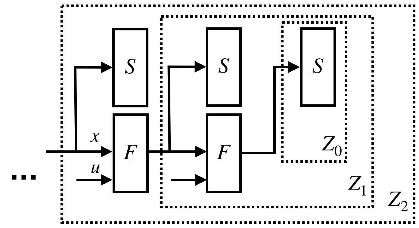
Figure 3: Safety control synthesis iteration (3) depicted as a sequence of sink interfaces.

Figure 3 shows a visualization of the safety game’s fixed point iteration from the point of view of relational interfaces. Starting from the right-most sink interface $S$ (equivalent to $Z_{0}$) the iteration (3) constructs a sequence of sink interfaces $Z_{1},Z_{2},...$ encoding relevant subsets of the state space. The numerous $S(x,{\varnothing})$ interfaces impose constraints and can be interpreted as monitors that raise errors if the safety constraint is violated.

3.3 Modifying the Control Synthesis Pipeline

Equation 10’s definition of ${\text{{cpre}}}(\cdot)$ is oblivious to the domains of variables $x,u$, and $x^{+}$. This generality is useful for describing a problem and serving as a blank template. Whenever problem structure exists, pipeline modifications refine the general algorithm into a form that reflects the specific problem instance. They also allow a user to inject implicit preferences into a problem and reduce computational bottlenecks or to refine a solution. The subsequent sections apply this philosophy to the abstraction-based control techniques from Section 1.1:

• Section 4: Coarsening interfaces reduces the computational complexity of a problem by throwing away fine grain information. The synthesis result is conservative but the degree of conservatism can be modified.

• Section 5: Refining interfaces decreases result conservatism. Refinement in combination with coarsening allows one to dynamically modulate the complexity of the problem as a function of multiple criteria such as the result granularity or minimizing computational resources.

• Section 6: If the dynamics or specifications are decomposable then the control predecessor operator can be broken apart to refect that decomposition.

These sections do more than simply reconstruct existing techniques in the language of relational interfaces. They uncover some implicit assumptions in existing tools and either remove them or make them explicit. Minimizing the number of assumptions ensures applicability to a diverse collection of systems and specifications and compatibility with future algorithmic modifications.

4 Interface Abstraction via Quantization

A key motivator behind abstraction-based control synthesis is that computing the game iterations from Equation 2 and Equation 3 exactly is often intractable for high-dimensional nonlinear dynamics. Termination is also not guaranteed. Quantizing (or “abstracting”) continuous interfaces into a finite counterpart ensures that each predicate operation of the game terminates in finite time but at the cost of the solution’s precision. Finer quantization incurs a smaller loss of precision but can cause the memory and computational requirements to store and manipulate the symbolic representation to exceed machine resources.

This section first introduces the notion of interface abstraction as a refinement relation. We define the notion of a quantizer and show how it is a simple generalization of many existing quantizers in the abstraction-based control literature. Finally, we show how one can inject these quantizers anywhere in the control synthesis pipeline to reduce computational bottlenecks.

4.1 Theory of Abstract Interfaces

While a controller synthesis algorithm can analyze a simpler model of the dynamics, the results have no meaning unless they can be extrapolated back to the original system dynamics. The following interface refinement condition formalizes a condition when this extrapolation can occur.

Definition 6 (Interface Refinement [22])

Let $F(i,o)$ and $\hat{F}(\hat{i},\hat{o})$ be interfaces. $\hat{F}$ is an abstraction of $F$ if and only if $i\equiv\hat{i}$, $o\equiv\hat{o}$, and

$$\text{{nb}}(\hat{F}) \Rightarrow\text{{nb}}(F)$$ (15)

$$\left(\text{{nb}}(\hat{F})\and F\right) \Rightarrow\hat{F}$$ (16)

are valid formulas. This relationship is denoted by $\hat{F}\preceq F$.

Definition 6 imposes two main requirements between a concrete and abstract interface. Equation 15 encodes the condition where if $\hat{F}$ accepts an input, then $F$ must also accept it; that is, the abstract component is more aggressive with rejecting invalid inputs. Second, if both systems accept the input then the abstract output set is a superset of the concrete function’s output set. The abstract interface is a conservative representation of the concrete interface because the abstraction accepts fewer inputs and exhibits more non-deterministic outputs. If both the interfaces are sink interfaces, then $\hat{F}\preceq F$ reduces down to $\hat{F}\subseteq F$ when $F,\hat{F}$ are interpreted as sets. If both are source interfaces then the set containment direction is flipped and $\hat{F}\preceq F$ reduces down to $F\subseteq\hat{F}$.

The refinement relation satisfies the required reflexivity, transitivity, and antisymmetry properties to be a partial order [22] and is depicted in Figure 4. This order has a bottom element $\bot$ which is a universal abstraction. Conveniently, the bottom element $\bot$ signifies both boolean false and the bottom of the partial order. This interface blocks for every potential input. In contrast, Boolean $\top$ plays no special role in the partial order. While $\top$ exhibits totally non-deterministic outputs, it also accepts inputs. A blocking input is considered “worse” than non-deterministic outputs in the refinement order.

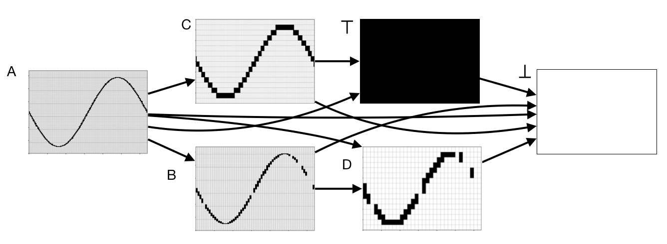
Figure 4: Example depiction of the refinement partial order. Each small plot on the depicts input-output pairs that satisfy an interface’s predicate. Inputs (outputs) vary along the horizontal (vertical) axis. Because $B$ blocks on some inputs but $A$ accepts all inputs $B\preceq A$. Interface $C$ exhibits more output non-determinism than $A$ so $C\preceq A$. Similarly $D\preceq B$, $D\preceq C$ , $\top\preceq C$, etc. Note that $B$ and $C$ are incomparable because $C$ exhibits more output non-determinism and $B$ blocks for more inputs. The false interface $\bot$ is a universal abstraction, while $\top$ is incomparable with $B$ and $D$.

The refinement relation $\preceq$ encodes a direction of conservatism such that any reasoning done over the abstract models is sound and can be generalized to the concrete model.

Theorem 4.1 (Informal Substitutability Result [22])

For any input that is allowed for the abstract model, the output behaviors exhibited by an abstract model contains the output behaviors exhibited by the concrete model.

If a property on outputs has been established for an abstract interface, then it still holds if the abstract interface is replaced with the concrete one. Informally, the abstract interface is more conservative so if a property holds with the abstraction then it must also hold for the true system. All aforementioned interface operators preserve the properties of the refinement relation of Definition 6, in the sense that they are monotone with respect to the refinement partial order.

Theorem 4.2 (Composition Preserves Refinement [22])

Let $\hat{A}\preceq A$ and $\hat{B}\preceq B$. If the composition is well defined, then $\text{{comp}}(\hat{A},\hat{B})\preceq\text{{comp}}(A,B)$.

Theorem 4.3 (Output Hiding Preserves Refinement [22])

If $A\preceq B$, then $\text{{ohide}}(w,A)\preceq\text{{ohide}}(w,B)$ for any variable $w$.

Theorem 4.4 (Input Hiding Preserves Refinement)

If $A,B$ are both sink interfaces and $A\preceq B$, then $\text{{ihide}}(w,A)\preceq\text{{ihide}}(w,B)$ for any variable $w$.

Proofs for Theorems 4.2 and 4.3 are provided in [22]. Theorem 4.4’s proof is simple and is omitted. One can think of using interface composition and variable hiding to horizontally (with respect to the refinement order) navigate the space of all interfaces. The synthesis pipeline encodes one navigated path and monotonicity of these operators yields guarantees about the path’s end point. Composite operators such as ${\text{{cpre}}}(\cdot)$ chain together multiple incremental steps. Furthermore since the composition of monotone operators is itself a monotone operator, any composite constructed from these parts is also monotone. In contrast, the coarsening and refinement operators introduced later in Definition 8 and 10 respectively are used to move vertically and construct abstractions. The “direction” of new composite operators can easily be established through simple reasoning about the cumulative directions of their constituent operators.

4.2 Dynamically Coarsening Interfaces

In practice, the sequence of interfaces $Z_{i}$ generated during synthesis grows in complexity. This occurs even if the dynamics $F$ and the target/safe sets have compact representations (i.e., fewer nodes if using BDDs). Coarsening $F$ and $Z_{i}$ combats this growth in complexity by effectively reducing the amount of information sent between iterations of the fixed point procedure.

Spatial discretization or coarsening is achieved by use of a quantizer interface that implicitly aggregates points in a space into a partition or cover.

Definition 7

A quantizer $Q(i,o)$ is any interface that abstracts the identity interface $(i==o)$ associated with the signature $(i,o)$.

Quantizers decrease the complexity of the system representation and make synthesis more computationally tractable. A coarsening operator abstracts an interface by connecting it in series with a quantizer. Coarsening reduces the number of non-blocking inputs and increases the output non-determinism.

Definition 8 (Input/Output Coarsening)

Given an interface $F(i,o)$ and input quantizer $Q(\hat{i},i)$, input coarsening yields an interface with signature $(\hat{i},o)$.

$$\text{{icoarsen}}(F,Q(\hat{i},i)) =\text{{ohide}}(i,\text{{comp}}(Q(\hat{i},i),F))$$ (17)

Similarly, given an output quantizer $Q(o,\hat{o})$, output coarsening yields an interface with signature $(i,\hat{o})$.

$$\text{{ocoarsen}}(F,Q(o,\hat{o})) =\text{{ohide}}(o,\text{{comp}}(F,Q(o,\hat{o})))$$ (18)

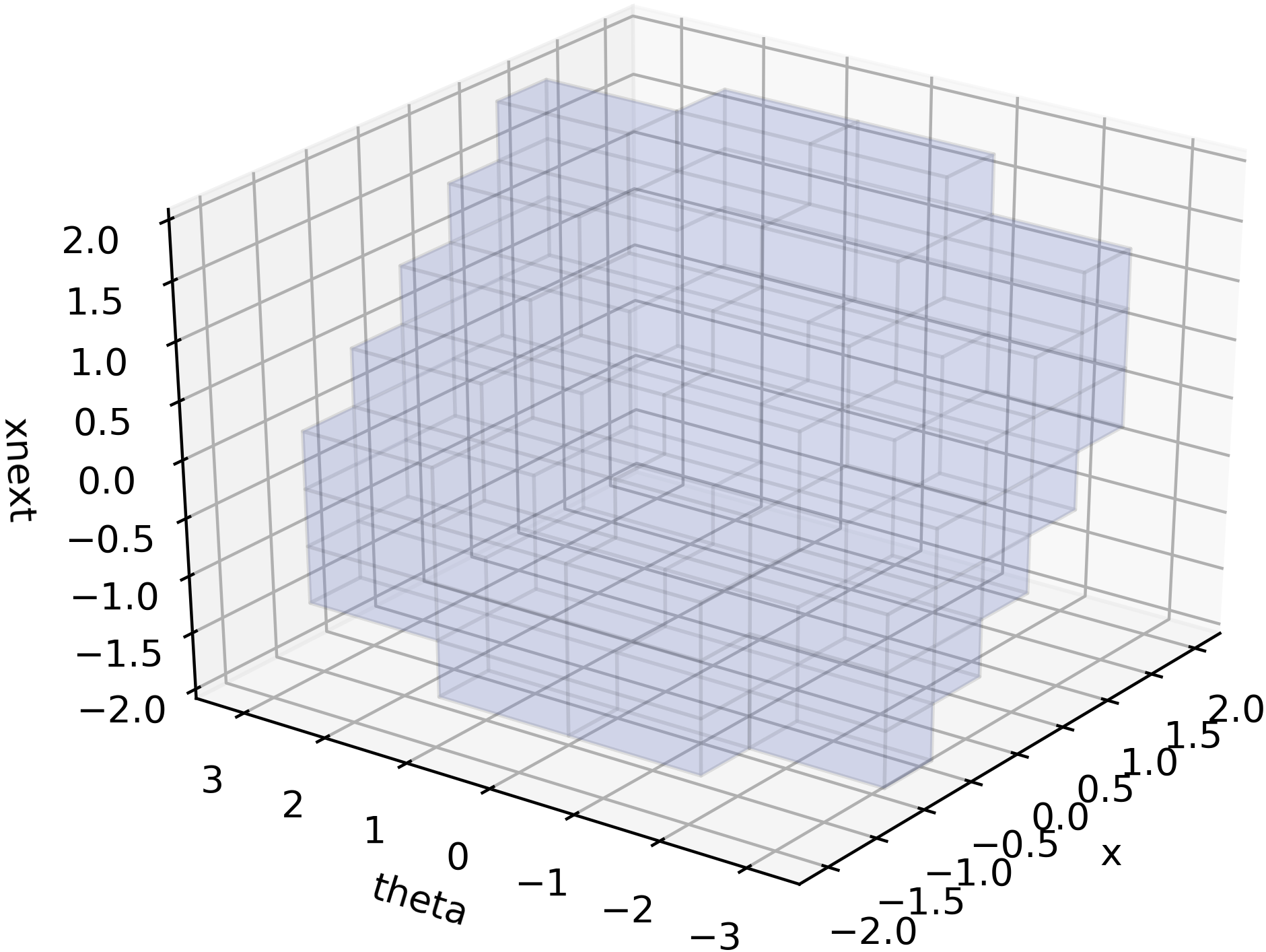
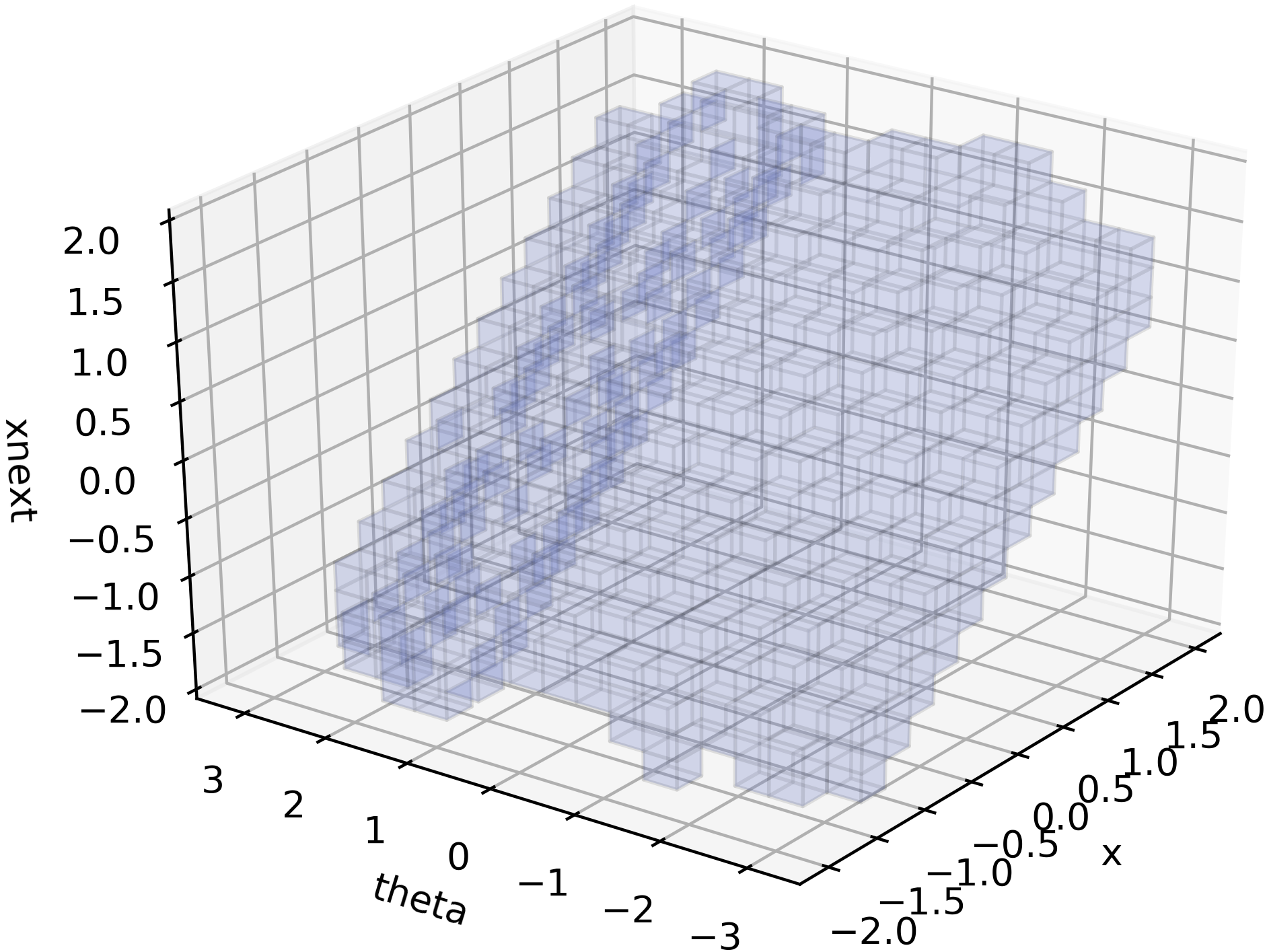
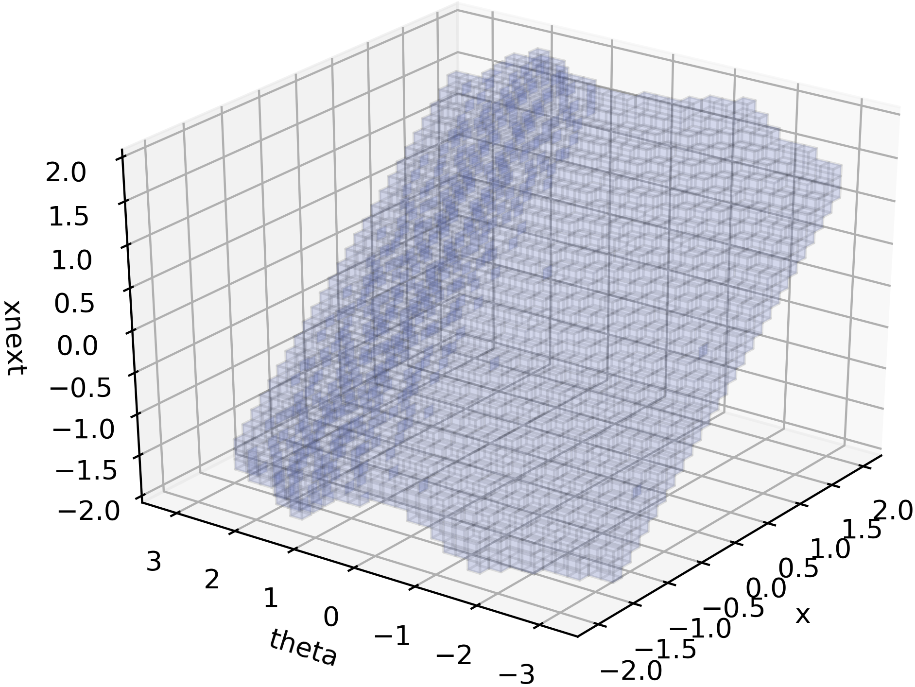
Figure 5: Coarsening of the $F_{x}$ interface to $2^{3},2^{4}$ and $2^{5}$ bins along each dimension for a fixed $v$ assignment. Interfaces are coarsened within milliseconds for BDDs but the runtime depends on the finite abstraction’s data structure representation.

Figure 5 depicts how coarsening reduces the information required to encode a finite interface. Section 8.1 in the appendix shows how the dynamic precision quantizer in [1] is implemented.

The corollary below shows that quantizers can be seamlessly integrated into the synthesis pipeline while preserving the refinement order. It readily follows from Theorem 4.2, Theorem 4.3, and the quantizer definition.

Corollary 1

Input and output coarsening operations(17) and (18) are monotone operations with respect to the interface refinement order $\preceq$.

It is difficult to know a priori where a specific problem instance lies along the spectrum between mathematical precision and computational efficiency. It is then desirable to coarsen dynamically in response to runtime conditions rather than statically beforehand.

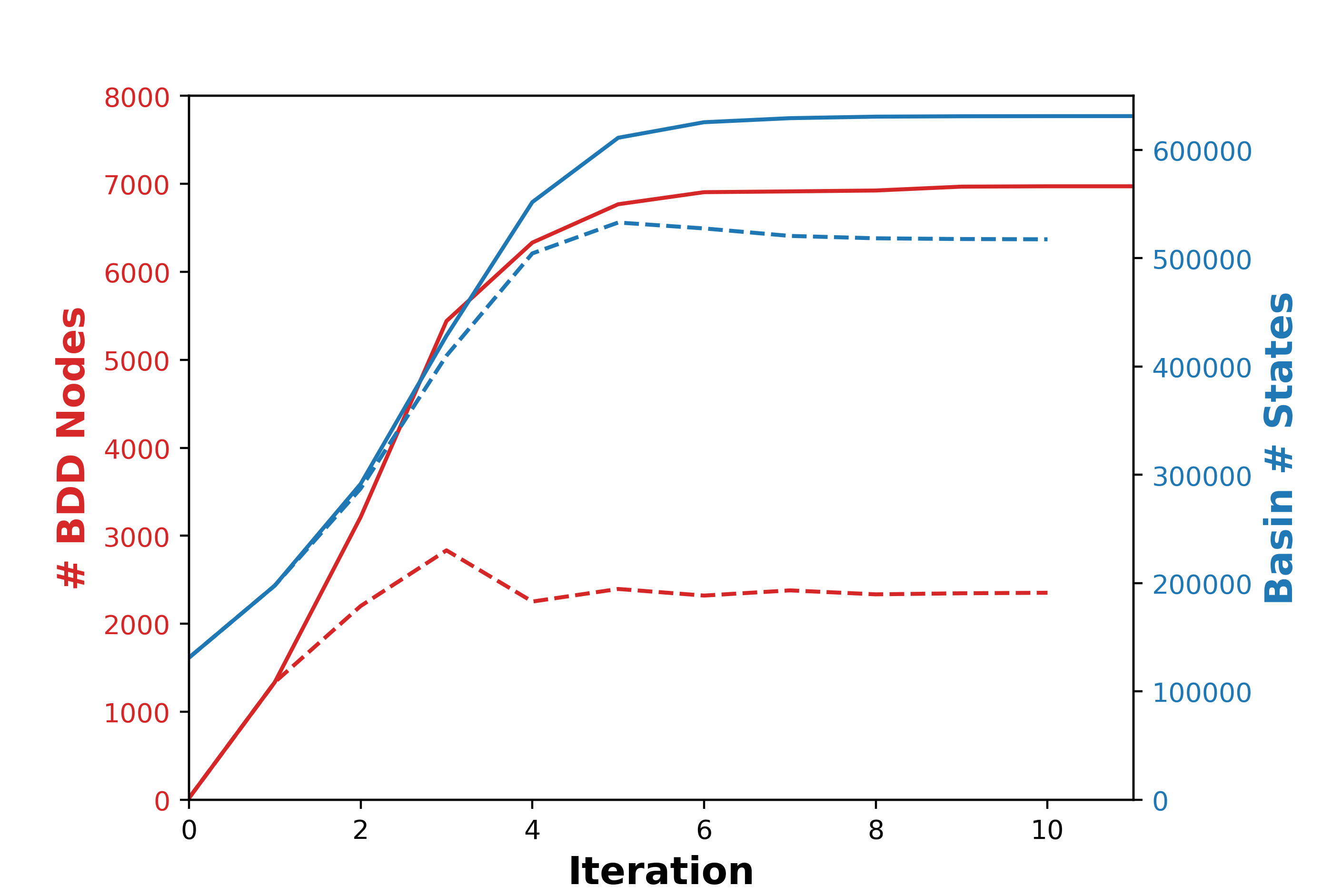
Figure 6: Number of BDD nodes (red) and number of states in reach basin (blue) with respect to the reach game iteration with a greedy quantization. The solid lines result from the unmodified game with no coarsening heuristic. The dashed lines result from greedy coarsening whenever the winning region exceeds 3000 BDD nodes.

Coarsening heuristics for reach games include:

• Downsampling with progress [7]: Initially use coarser system dynamics to rapidly identify a coarse reach basin. Finer dynamics are used to construct a more granular set whenever the coarse iteration “stalls”. In [7] only the $Z_{i}$ are coarsened during synthesis. We enable the dynamics $F$ to be as well.

• Greedy quantization: Selectively coarsening along certain dimensions by checking at runtime which dimension, when coarsened, would cause $Z_{i}$ to shrink the least. This reward function can be leveraged in practice because coarsening is computationally cheaper than composition. For BDDs, the winning region can be coarsened until the number of nodes reduces below a desired threshold. Figure 6 shows this heuristic being applied to reduce memory usage at the expense of answer fidelity. A fixed point is not guaranteed as long as quantizers can be dynamically inserted into the synthesis pipeline, but is once quantizers are always inserted at a fixed precision.

The most common quantizer in the literature never blocks and only increases non-determinism (such quantizers are called “strict” in [18][19]). If a quantizer is interpreted as a partition or cover, this requirement means that the union must be equal to an entire space. Definition 7 relaxes that requirement so the union can be a subset instead. It also hints at other variants such as interfaces that don’t increase output non-determinism but instead block for more inputs.

5 Refining System Dynamics

Shared refinement [22] is an operation that takes two interfaces and merges them into a single interface. In contrast to coarsening, it makes interfaces more precise. Many tools construct system abstractions by starting from the universal abstraction $\bot$, then iteratively refining it with a collection of smaller interfaces that represent input-output samples. This approach is especially useful if the canonical concrete system is a black box function, Simulink model, or source code file. These representations do not readily lend themselves to the predicate operations or be coarsened directly. We will describe later how other tools implement a restrictive form of refinement that introduces unnecessary dependencies.

Interfaces can be successfully merged whenever they do not contain contradictory information. The shared refinability condition below formalizes when such a contradiction does not exist.

Definition 9 (Shared Refinability [22])

Interfaces $F_{1}(i,o)$ and $F_{2}(i,o)$ with identical signatures are shared refinable if

$$\left(\text{{nb}}(F_{1})\and\text{{nb}}(F_{2})\right)\Rightarrow{\exists o}(F_{1}\and F_{2})$$ (19)

For any inputs that do not block for all interfaces, the corresponding output sets must have a non-empty intersection. If multiple shared refinable interfaces, then they can be combined into a single one that encapsulates all of their information.

Definition 10 (Shared Refinement Operation [22])

The shared refinement operation combines two shared refinable interfaces $F_{1}$ and $F_{2}$, yielding a new identical signature interface corresponding to the predicate

$$\text{{refine}}(F_{1},F_{2})=(\text{{nb}}(F_{1})\vee\text{{nb}}(F_{2}))\and(\text{{nb}}(F_{1})\Rightarrow F_{1})\and(\text{{nb}}(F_{2})\Rightarrow F_{2}).$$ (20)

The left term expands the set of accepted inputs. The right term signifies that if an input was accepted by multiple interfaces, the output must be consistent with each of them. The shared refinement operation reduces to disjunction for sink interfaces and to conjunction for source interfaces.

Shared refinement’s effect is to move up the refinement order by combining interfaces. Given a collection of shared refinable interfaces, the shared refinement operation yields the least upper bound with respect to the refinement partial order in Definition 6. Violation of (19) can be detected if the interfaces fed into $\text{{refine}}(\cdot)$ are not abstractions of the resulting interface.

5.1 Constructing Finite Interfaces through Shared Refinement

A common method to construct finite abstractions is through simulation and overapproximation of forward reachable sets. This technique appears in tools such as PESSOA [12], SCOTS [19], MASCOT [7], ROCS [9] and ARCS [4]. By covering a sufficiently large portion of the interface input space, one can construct larger composite interfaces from smaller ones via shared refinement.

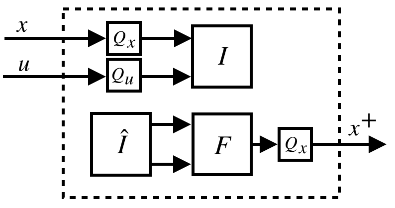
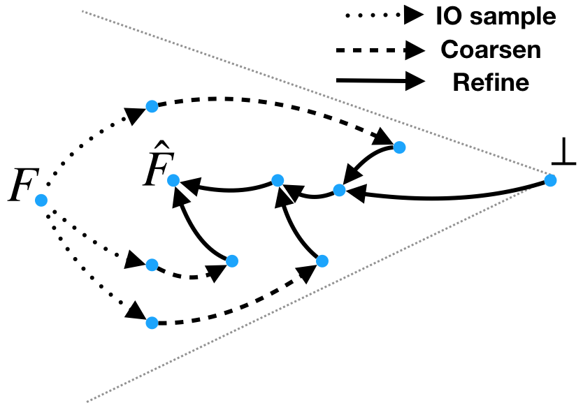
Figure 7: (Left) Result of sample and coarsen operations for control system interface $F(x\cup u,x^{+})$. The $I$ and $\hat{I}$ interfaces encode the same predicate, but play different roles as sink and source. (Right) Visualization of finite abstraction as traversing the refinement partial order. Nodes represent interfaces and edges signify data dependencies for interface manipulation operators. Multiple refine edges point to a single node because refinement combines multiple interfaces. Input-output (IO) sample and coarsening are unary operations so the resulting nodes only have one incoming edge. The concrete interface $F$ refines all others, and the final result is an abstraction $\hat{F}$.

Smaller interfaces are constructed by sampling regions of the input space and constructing an input-output pair. In Figure 7’s left half, a sink interface $I(x\cup u,{\varnothing})$ acts as a filter. The source interface $\hat{I}({\varnothing},x\cup u)$ composed with $F(x\cup u,x^{+})$ prunes any information that is outside the relevant input region. The original interface refines any sampled interface. To make samples finite, interface inputs and outputs are coarsened. An individual sampled abstraction is not useful for synthesis because it is restricted to a local portion of the interface input space. After sampling many finite interfaces are merged through shared refinement. The assumption $\hat{I}_{i}\Rightarrow\text{{nb}}(F)$ encodes that the dynamics won’t raise an error when simulated and is often made implicitly. Figure 7’s right half depicts the sample, coarsen, and refine operations as methods to vertically traverse the interface refinement order.

Critically, $\text{{refine}}(\cdot)$ can be called within the synthesis pipeline and does not assume that the sampled interfaces are disjoint. Figure 8 shows the results from refining the dynamics with a collection of state-control hyper-rectangles that are randomly generated via uniformly sampling their widths and offsets along each dimension. These hyper-rectangles may overlap. If the same collection of hyper-rectangles were used in MASCOT, SCOTS, ARCS, or ROCS then this would yield a much more conservative abstraction of the dynamics because their implementations are not robust to overlapping or misaligned samples. PESSOA and SCOTS circumvent this issue altogether by enforcing disjointness with an exhaustive traversal of the state-control space, at the cost of unnecessarily coupling the refinement and sampling procedures. The lunar lander contained in Section 8.2 of the appendix embraces overlapping and uses two mis-aligned grids to construct a grid partition with $p^{N}$ elements with only $p^{N}(\frac{1}{2})^{N-1}$ samples (where $p$ is the number of bins along each dimension and $N$ is the interface input dimension). This technique introduces a small degree of conservatism but its computational savings typically outweigh this cost.

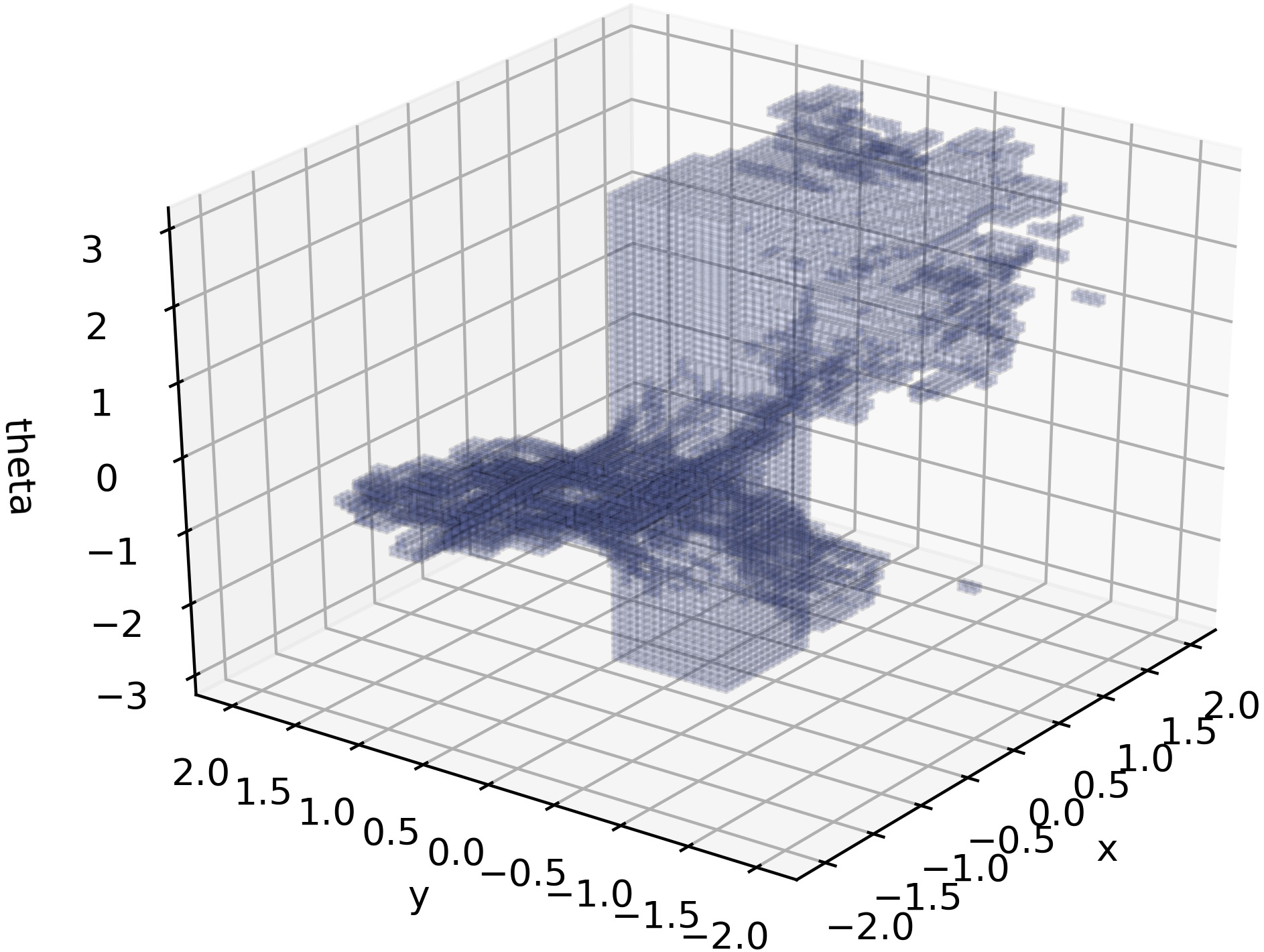
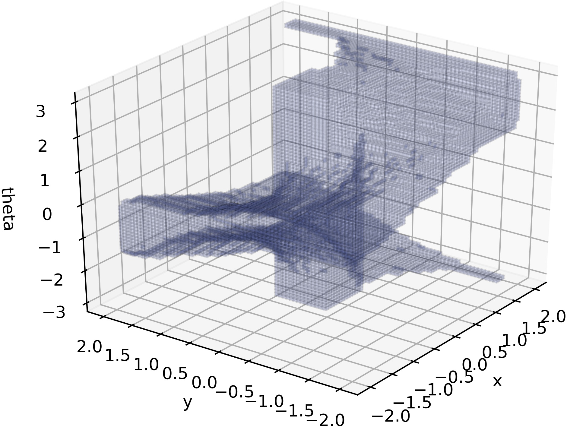
Figure 8: The number of states in the computed reach basin grows with the number of random samples. The vertical axis is lower bounded by the number of states in the target $131k$ and upper bounded by $631k$, the number of states using an exhaustive traversal. Naive implementations of the exhaustive traversal would require $12$ million samples. The right shows basins for 3000 (top) and 6000 samples (bottom).

6 Decomposed Control Predecessor

A decomposed control predecessor is available whenever the system state space consists of a Cartesian product and the dynamics are decomposed component-wise such as $F_{x},F_{y}$, and $F_{\theta}$ for the Dubins vehicle. This property is common for continuous control systems over Euclidean spaces. While one may construct $F$ directly via the abstraction sampling approach, it is often intractable for larger dimensional systems. A more sophisticated approach abstracts the lower dimensional components $F_{x},F_{y}$, and $F_{\theta}$ individually, computes $F=\text{{comp}}(F_{x},F_{y},F_{\theta})$, then feeds it to the monolithic ${\text{{cpre}}}(\cdot)$ from Proposition 1. This section’s approach is to avoid computing $F$ at all and decompose the monolithic ${\text{{cpre}}}(\cdot)$. It operates by breaking apart the term $\text{{ohide}}(x^{+},\text{{comp}}(F,Z))$ in such a way that it respects the decomposition structure.

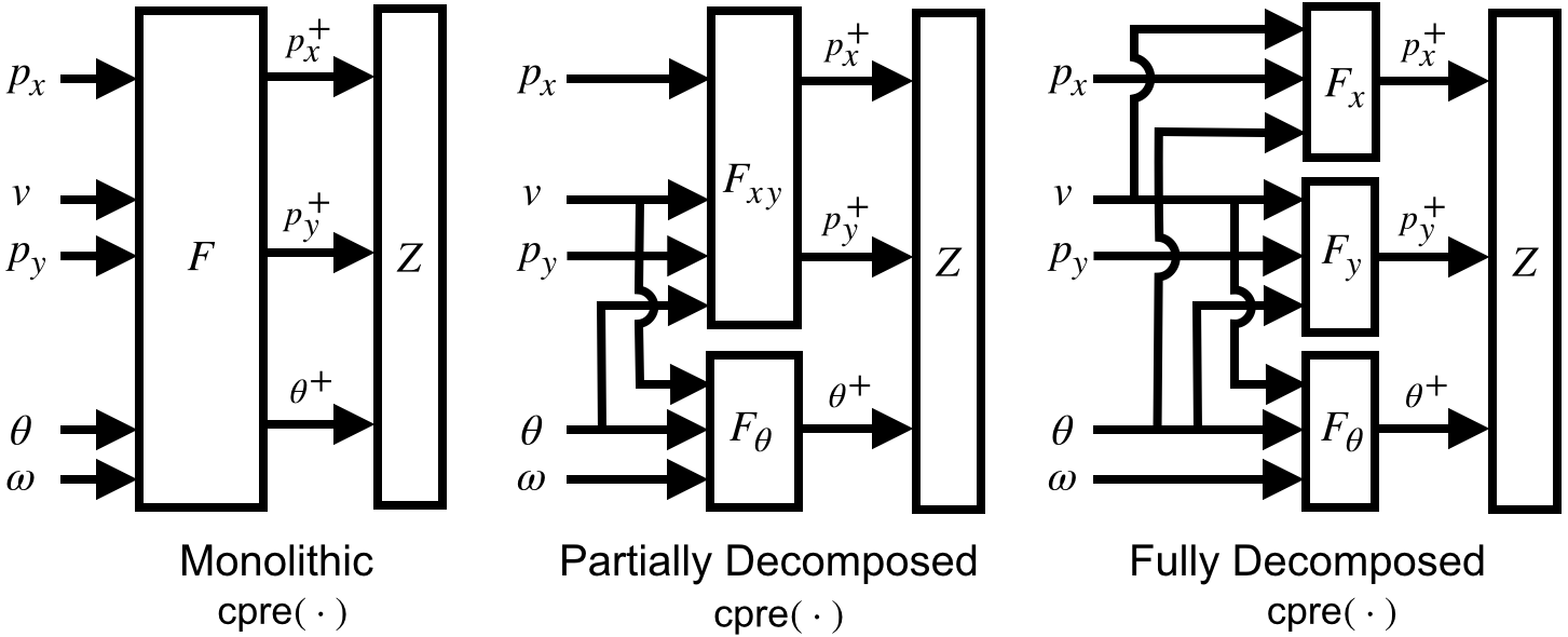
Decomposition	Parallel Compose	Reach Game
	Runtime (s)	Runtime (s)
$F$ (Monolithic)	0.56	103.09
$F_{y\theta},F_{x}$ (Partially Decomp.)	0.02	28.31
$F_{x\theta},F_{y}$ (Partially Decomp.)	0.01	28.71
$F_{xy},F_{\theta}$ (Partially Decomp.)	0.06	10.61
$F_{x},F_{y},F_{\theta}$ (Fully Decomp.)	n/a	4.42

Figure 9: A monolithic ${\text{{cpre}}}(\cdot)$ incurs unnecessary pre-processing and synthesis runtime costs for the Dubins vehicle reach game. Each variant of ${\text{{cpre}}}(\cdot)$ above composes the interfaces $F_{x},F_{y}$ and $F_{\theta}$ in different permutations. For example, $F_{xy}$ represents $\text{{comp}}(F_{x},F_{y})$ and $F$ represents $\text{{comp}}(F_{x},F_{y},F_{\theta})$.

For the Dubins vehicle example $\text{{ohide}}(x^{+},\text{{comp}}(F,Z))$ is replaced with

$$\text{{ohide}}(p_{x}^{+},\text{{comp}}(F_{x},\text{{ohide}}(p_{y}^{+},\text{{comp}}(F_{y},\text{{ohide}}(\theta^{+},\text{{comp}}(F_{\theta},Z))))))$$

yielding a sink interface with inputs $p_{x},p_{y},v,\theta$, and $\omega$. This representation and the original $\text{{ohide}}(x^{+},\text{{comp}}(F,Z))$ are equivalent because $\text{{comp}}(\cdot)$ is associative and interfaces do not share outputs $x^{+}\equiv\{p_{x}^{+},p_{y}^{+},\theta^{+}\}$. Figure 9 shows multiple variants of ${\text{{cpre}}}(\cdot)$ and improved runtimes when one avoids preemptively constructing the monolithic interface. The decomposed ${\text{{cpre}}}(\cdot)$ resembles techniques to exploit partitioned transition relations in symbolic model checking [5].

No tools from Section 1.1 natively support decomposed control predecessors. We’ve shown a decomposed abstraction for components composed in parallel but this can also be generalized to series composition to capture, for example, a system where multiple components have different temporal sampling periods.

7 Conclusion

Tackling difficult control synthesis problems will require exploiting all available structure in a system with tools that can flexibly adapt to an individual problem’s idiosyncrasies. This paper lays a foundation for developing an extensible suite of interoperable techniques and demonstrates the potential computational gains in an application to controller synthesis with finite abstractions. Adhering to a simple yet powerful set of well-understood primitives also constitutes a disciplined methodology for algorithm development, which is especially necessary if one wants to develop concurrent or distributed algorithms for synthesis.

8 Appendix

8.1 Dynamic Precision Quantization

Certain data structures like trees or binary decision diagrams are natural candidates for encoding hierarchical decompositions of spaces. A sequence of bits can be used to traverse that data structure to arrive at a subset of that space. More bits allow one to specify finer granularity sets. As an illustrative example, consider an interval $[0,1]$ that is to be covered. Let $N$ represent a number of bits to construct a cover of $[0,1]$, and assign a unique bit sequence to identify each set in the cover. Figure 10 depicts for varying $N$ how an interval can be covered by a collection of small intervals, while minimizing overlaps. A greater $N$ signifies that the cover can be constructed with finer intervals. A bit vector of length $N$ can be used to specify an interval of width $2^{-N}$. If $N=\infty$, then any value in $[0,1]$ can be encoded via the infinite weighted sum $\sum_{k=1}^{\infty}2^{-k}o_{k}$. For $N=0$, the interval is $[0,1]$ itself. Figure 10 implicitly appends don’t care terms $-$ to the end of bit vectors. This allows finite length bit vectors (intervals) to be identical to the disjunction (union) of longer bit vectors (smaller intervals) with a common prefix.

A quantizer acts by truncating a bit vector to a specified finite number of bits and outputting the result. The effect of truncating bits is to implicitly widen or coarsen that interval. A quantizer $Q_{N}(o,\hat{o})$ that only retains the first $N$ bits satisfies the following formula and is depicted in Figure 10

$$Q_{N}(o,\hat{o}) =Q_{N}(o_{1}\cup\ldots,\hat{o}_{1}\cup\ldots)=\bigwedge_{k=1}^{N}\left(o_{k}==\hat{o}_{k}\right).$$ (21)

$N=0$	$---$
$N=1$	$\bot--$		$\top--$
$N=2$	$\bot\bot-$	$\bot\top-$	$\top\bot-$	$\top\top-$
$N>2$	⋮

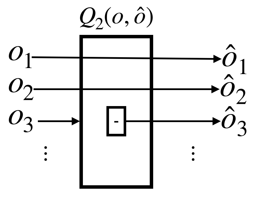
Figure 10: (Left) Varying length $N$ of a bit vector leads to different granularity covers of an interval. The don’t care term “$-$” signifies that the value of a certain bit does not matter. Bit vectors of finite length are implicitly appended with an infinite sequence of don’t cares. (Right) A bit quantizer in Equation 21 with $N=2$. Higher significant bits are outputted but are replaced with a don’t care term “$-$” that can non-deterministically be true or false.

The quantizer implicitly receives and emits infinite bit sequences but only depends on the most significant bits. It ignores higher precision input bits and non-deterministically assigns values to higher precision output bits. The input and output domains have identical cardinality but the quantizer is not a function due to the non-deterministic output. It is easy to see that for two quantizers $Q_{N},Q_{M}$ with precisions $N,M\in\mathbb{N}\cup\{\infty\}$ and $N\leq M$ the relation $Q_{N}\preceq Q_{M}$ holds. A collection of quantizers composed in series also yields a single quantizer with the minimum precision.

Applying the quantizer definition above to the output coarsening and input coarsening operations yield insightful results.

Example 1 (Output Quantizer)

Consider an interface $F(i,o)$ where $o=o_{1}\cup o_{2}\cup\ldots$ is a composite variable representing an infinite bit vector. Let $o_{msb}=o_{1}\cup\ldots\cup o_{N}$ be the most significant bits and $o_{lsb}=o_{N+1}\cup\ldots$ be the least significant bits.

$$\text{{ocoarsen}}(M,Q(o,\hat{o}))$$ (22)

$$=\text{{ohide}}(o,\text{{comp}}(M,Q(o,\hat{o})))$$ (23)

$$={\exists o}\left(\bigwedge_{k=1}^{N}\left(o_{k}==\hat{o_{k}}\right)\and F\and{\forall o}\left(F\Rightarrow{\exists\hat{o}}\left(\bigwedge_{k=1}^{N}\left(o_{k}==\hat{o_{k}}\right)\right)\right)\right)$$ (24)

$$={\exists o}\left(\bigwedge_{k=1}^{N}\left(o_{k}==\hat{o}_{k}\right)\and F\and\top\right)$$ (25)

$$={\exists o}_{msb}\left(\bigwedge_{k=1}^{N}\left(o_{k}==\hat{o}_{k}\right)\and{\exists o_{lsb}}F\right)$$ (26)

The last predicate has signature $(i,\hat{o}_{msb})$ and is equivalent to the predicate ${\exists o_{lsb}}F$ after the $o$ bit are replaced with their respective $\hat{o}$ bits. In other words, the output non-determinism is increased.

The input quantizer is more complicated than output quantization.

Example 2 (Input Quantizer)

Consider an interface $F(i,o)$ where $i\equiv i_{1}\cup i_{2}\cup\ldots$ is a composite variable representing an infinite bit vector. Let $i_{msb}=i_{1}\cup\ldots i_{N}$ be the most significant bits and $i_{lsb}=i_{N+1}\cup\ldots$ be the least significant bits. The input coarsening operator yields the following equivalent prediates.

$$\text{{icoarsen}}(F,Q(\hat{i},i))$$ (27)

$$=\text{{ihide}}(i,\text{{comp}}(Q(\hat{i},i),F))$$ (28)

$$={\exists i}\left(\bigwedge_{k=1}^{N}\left(i_{k}==\hat{i}_{k}\right)\and F\and{\forall i}\left(\bigwedge_{k=1}^{N}\left(i_{k}==\hat{i}_{k}\right)\Rightarrow\text{{nb}}(F)\right)\right)$$ (29)

$$={\exists i}\left(\bigwedge_{k=1}^{N}\left(i_{k}==\hat{i}_{k}\right)\and F\and{\forall i}_{msb}\left(\bigwedge_{k=1}^{N}\left(i_{k}==\hat{i}_{k}\right)\Rightarrow{\forall i}_{lsb}\text{{nb}}(F)\right)\right)$$ (30)

$$={\exists i}\left(\bigwedge_{k=1}^{N}\left(i_{k}==\hat{i}_{k}\right)\and F\right)\and{\forall i}_{msb}\left(\bigwedge_{k=1}^{N}\left(i_{k}==\hat{i}_{k}\right)\Rightarrow{\forall i}_{lsb}\text{{nb}}(F)\right)$$ (31)

$$={\exists i}_{msb}\left(\bigwedge_{k=1}^{N}\left(i_{k}==\hat{i}_{k}\right)\and{\exists i}_{lsb}F\right)\and{\forall i}_{msb}\left(\bigwedge_{k=1}^{N}\left(i_{k}==\hat{i}_{k}\right)\Rightarrow{\forall i}_{lsb}\text{{nb}}(F)\right)$$ (32)

The last predicate has signature $(\hat{i}_{msb},o)$ and is equivalent to the predicate ${\exists i}_{lsb}F\and{\forall i_{lsb}}(\text{{nb}}(F))$ after all $i$ bits are replaced with their respective $\hat{i}$ bits. The ${\exists i}_{lsb}F$ term increases output non-determinism by taking a union of outputs generated by different lower significant bit assignments. Term ${\forall i_{lsb}}(\text{{nb}}(F))$ imposes that if some input assignments can block, then all other input assignments with identical most significant bits are also blocked.

Remark 1

A multi-dimensional quantizer simply consists of multiple scalar quantizers. The encoding for the interval $[0,1]$ can be rescaled to an interval $[a,b]$. Additional care needs to be taken for non-powers of two, and overflow bits can be added to extend to $\mathbb{R}$.

8.2 Lunar Lander

We consider the lunar lander from OpenAI gym [3], a python simulation environment for reinforcement learning research. The lander is set up within a physics simulation engine and has six continuous state dimensions and two continuous input dimensions. After some minor modifications , we identified the following discrete time dynamics

$$p_{x}^{+} =p_{x}+.01031v_{x}$$ (33)

$$p_{y}^{+} =p_{y}+.0225v_{y}$$ (34)

$$v_{x}^{+} =v_{x}-.0539u_{1}\sin(\theta)+.0106u_{2}\cos(\theta)$$ (35)

$$v_{y}^{+} =v_{y}+.0359u_{1}\cos(\theta)+.00707u_{2}\sin(\theta)-.0267$$ (36)

$$\theta^{+} =\theta+.05\omega$$ (37)

$$\omega^{+} =\omega-.05598u_{2}.$$ (38)

Control input $u_{1}\in\{0\}\cup[.5,1]$ represents a main thruster mounted on the bottom of the lander, and input $u_{2}\in[-1,-.5]\cup\{0\}\cup[.5,1]$ represents a pair of side thrusters. Only one side thruster can be activated at a time and both are aligned in such a way that they apply both a torque and a linear force when activated. Both thrusters can only apply impulses with magnitude greater than $0.5$ when activated. This limits the system’s ability to exert fine control over the system without resorting to high frequency chattering.

The continuous region of interest for our problem is $p_{x}\in[-1,1]$, $p_{y}\in[0,1.3]$, $v_{x}\in[-1,1]$, $v_{y}\in[-1,1]$, $\theta\in[-\frac{\pi}{5},\frac{\pi}{5}]$ and $\omega\in[-.6,.6]$. The discretized state space consists of $\sim$137 billion states obtained from a $256\times 256\times 64\times 64\times 32\times 16$ grid. Inputs are constrained to discrete sets $u_{1}\in\{0,.66,.83,1\}$ and $u_{2}\in\{-.5,0,.5\}$.

While one could construct interfaces associated with each equation (33)-(38), the positional components $p_{x}^{+}$ and $p_{y}^{+}$ would require finer grids than those above to capture a changing state over the short time horizon. Instead of using the one-step dynamics above, we instead use a sampled system with a period of 9 time steps. We refer to the interfaces associated with the unrolled dynamics with the names shown in Table 1. The time to construct all six interfaces was $430.5$ seconds. A reach objective with a target region $T$ is specified by

$$p_{x}\in[-.1,.1]\and p_{y}\in[1.2,1.3]\and\theta\in[-.15,.15]\and v_{y}\in[-8,.1]$$

which corresponds to 73 million states of the full dimensional space. We iterate a custom reach operator 20 iterations to construct a winning set with 344.6 million states. Trajectories reaching the target are depicted in Figure 11. The control synthesis runtime was 4194 seconds but a small portion of that includes applying the coarsening operation as detailed later. We applied the aforementioned decomposed predecessor and greedy coarsening heuristic and gradually increase the complexity threshhold from $10^{5}$ BDD nodes until a cap of $10^{6}$ nodes. For the lunar lander problem, many computers would run out of memory before the game solver reaches a fixed point. These abstraction and synthesis runtime numbers were achieved using additional techniques outlined below.

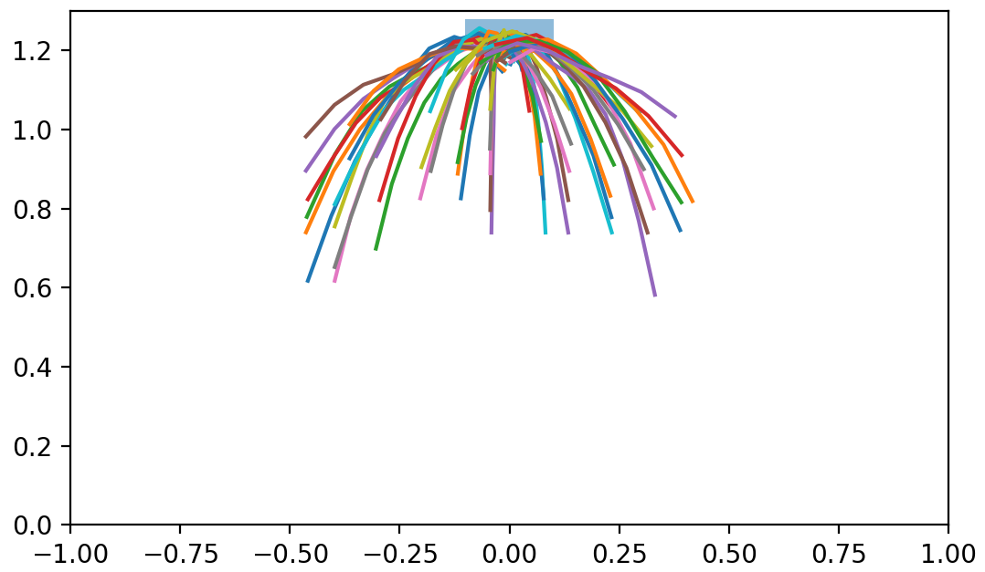
Figure 11: Two dimensional positional trajectories reaching a target set in blue.

Abstraction with Heterogeneous Grids: While sampling over a longer time horizon lets us use a coarser grid, it comes at the cost of increasing the number of interface inputs. States $\theta$ and $\omega$ at time $t=0$ can influence state $p_{x}$ at future time steps through their effect on $v_{x}$. While $p_{x}$ can depend on $\theta$ and $\omega$ over time, its sensitivity to those values is small over short horizons. Heterogeneous grids exploit this insight and allow small perturbations of $\theta$ and $\omega$ to be ignored. Table 1 shows how interface $F_{p_{x}}$ allocates less bits to those variables than interfaces $F_{\theta}$ and $F_{\omega}$, which are much more sensitive to the same perturbations over the same time horizon. Curiously, $F_{p_{x}}$ assigns zero bits to $\omega$. This signifies that it only assumes that $\omega\in[-.6,.6]$ but does not otherwise care what the specific value is due to the low sensitivity.

Interface	Output	Input
Name	Variable	Variables
$F_{p_{x}}$	$p_{x}^{+}\leftarrow 8$	$p_{x}\leftarrow 8$, $v_{x}\leftarrow 6$, $\theta\leftarrow 3$, $\omega\leftarrow 0$, $u_{1}$, $u_{2}$
$F_{p_{y}}$	$p_{y}^{+}\leftarrow 8$	$p_{y}\leftarrow 8$, $v_{y}\leftarrow 6$, $\theta\leftarrow 3$, $\omega\leftarrow 0$, $u_{1}$, $u_{2}$
$F_{v_{x}}$	$v_{x}^{+}\leftarrow 6$	$v_{x}\leftarrow 6$, $\theta\leftarrow 5$, $\omega\leftarrow 4$, $u_{1}$, $u_{2}$
$F_{v_{y}}$	$v_{y}^{+}\leftarrow 6$	$v_{y}\leftarrow 6$, $\theta\leftarrow 5$, $\omega\leftarrow 4$, $u_{1}$, $u_{2}$
$F_{\theta}$	$\theta^{+}\leftarrow 5$	$\theta\leftarrow 5$, $\omega\leftarrow 4$, $u_{2}$
$F_{\omega}$	$\omega^{+}\leftarrow 4$	$\omega\leftarrow 4$, $u_{2}$

Table 1: Each row represents an interface of the unrolled dynamics. The notation $p_{x}\leftarrow 8$ signifies that $p_{x}$ is a continuous variable and the interface has allocated $8$ bits to it. Different interfaces can have different views of the same variable, e.g. interface $F_{\omega}$ allocates $4$ bits to $\omega$ while $F_{p_{x}}$ allocates none. Inputs $u_{1}$ and $u_{2}$ are discrete so they do not adopt this notation.

Abstraction with Coarse Shifted Grids: Some interfaces can have up to a half million inputs with the granularity provided in Table 1. Instead of exhaustively iterating over all of them, we use the overlapping property of shared refinement to reduce the number of iterations while still inducing a grid of the desired granularity. Figure 12 depicts a simple two dimensional version of the iteration procedure where a higher granularity grid is constructed by two coarser grids that are offset from one another. This technique generally yields a more conservative abstraction than the one obtained by a full granularity traversal, but leads to a reduction in abstraction runtime. An overapproximation of a forward reachable set was represented as a hyper-rectangle. Simple interval analysis techniques could be applied for the one-step dynamics, and iterated over $9$ time steps. This technique is not implemented in prior tools.

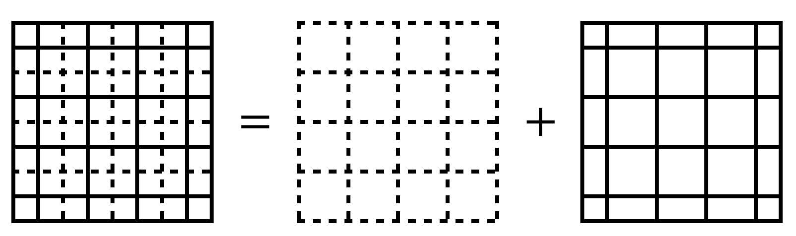
Figure 12: A $8\times 8$ partition induced by overlaying a $4\times 4$ partition and a $5\times 5$ partition. Note that $4^{2}+5^{2}<8^{2}$. For grids of dimension $N$, this technique reduces the number of iterations by a factor of roughly $2^{N-1}$. An initial factor of roughly $2^{N}$ is achieved by doubling the cell width along each dimension, but iterating over two grids reduces this factor to $2^{N-1}$.

Example 3 illustrates the key idea behind how one can leverage overlapping input sets to implicitly create more discrete states than the number of loop iterations.

Example 3

For $j\in\{1,2\}$, let $I_{j}$ be a sink and $O_{j}$ be a source. Composing these in parallel yields two input-output interfaces $I_{1}\and O_{1}$ and $I_{2}\and O_{2}$. These sink and source interfaces represent the ones from Figure 7’s left. The shared refinement interface outputted by $\text{{refine}}(\cdot)$ has a predicate

$$(I_{1}\vee I_{2})\and(I_{1}\Rightarrow O_{1})\and(I_{2}\Rightarrow O_{2})$$ (39)

that is logically equivalent to

$$(I_{1}\and I_{2}\and O_{1}\and O_{2})\vee(I_{1}\and\neg I_{2}\and O_{1})\vee(\neg I_{1}\and I_{2}\and O_{2}).$$ (40)

If $I_{1}$ and $I_{2}$ correspond to disjoint sets, then this simplifies to a disjunction

$$(I_{1}\and O_{1})\vee(I_{2}\and O_{2})$$ (41)

because $I_{1}\and I_{2}\Leftrightarrow\bot$, $I_{1}\Rightarrow\neg I_{2}$ and $I_{2}\Rightarrow\neg I_{1}$. Disjointness is imposed by assumption in PESSOA and SCOTS, which iterate over a partition of the space. If $I_{1}$ and $I_{2}$ are not disjoint, then (40) can be viewed as three reach set overapproximations $O_{1}\and O_{2}$, $O_{1}$ and $O_{2}$ for three respective disjoint input sets $I_{1}\and I_{2}$, $\neg I_{1}\and I_{2}$, and $I_{1}\and\neg I_{2}$. By leveraging overlapping input domains, $\text{{refine}}(\cdot)$ has generated three discrete states despite only being provided two interfaces $I_{1}\and O_{1}$ and $I_{2}\and O_{2}$.

References

- [1] https://github.com/ericskim/redax/tree/CAV19.
- [2] T. Basar and G. J. Olsder. Dynamic noncooperative game theory, volume 23. Siam, 1999.
- [3] G. Brockman, V. Cheung, L. Pettersson, J. Schneider, J. Schulman, J. Tang, and W. Zaremba. Openai gym. arXiv preprint arXiv:1606.01540, 2016.
- [4] O. L. Bulancea, P. Nilsson, and N. Ozay. Nonuniform abstractions, refinement and controller synthesis with novel BDD encodings. CoRR, abs/1804.04280, 2018.
- [5] J. Burch, E. Clarke, and D. Long. Symbolic model checking with partitioned transition relations. 1991.
- [6] F. Gruber, E. Kim, and M. Arcak. Sparsity-aware finite abstraction. In 2017 IEEE 56th Conference on Decision and Control (CDC), Dec 2017.
- [7] K. Hsu, R. Majumdar, K. Mallik, and A.-K. Schmuck. Multi-layered abstraction-based controller synthesis for continuous-time systems. In Proceedings of the 21st International Conference on Hybrid Systems: Computation and Control (Part of CPS Week), HSCC ’18, pages 120–129, New York, NY, USA, 2018. ACM.
- [8] H. K. Khalil. Nonlinear systems, volume 3.
- [9] Y. Li and J. Liu. Rocs: A robustly complete control synthesis tool for nonlinear dynamical systems. In Proceedings of the 21st International Conference on Hybrid Systems: Computation and Control (Part of CPS Week), HSCC ’18, pages 130–135, New York, NY, USA, 2018. ACM.
- [10] J. Liu. Robust abstractions for control synthesis: Completeness via robustness for linear-time properties. In Proceedings of the 20th International Conference on Hybrid Systems: Computation and Control, HSCC ’17, pages 101–110, New York, NY, USA, 2017. ACM.
- [11] R. Majumdar. Symbolic algorithms for verification and control. PhD thesis, University of California, Berkeley, 2003.
- [12] M. Mazo Jr, A. Davitian, and P. Tabuada. Pessoa: A tool for embedded controller synthesis. In International Conference on Computer Aided Verification, pages 566–569. Springer, 2010.
- [13] P. J. Meyer, A. Girard, and E. Witrant. Compositional abstraction and safety synthesis using overlapping symbolic models. IEEE Transactions on Automatic Control, 2017, accepted.
- [14] S. Mouelhi, A. Girard, and G. Gössler. CoSyMA: A Tool for Controller Synthesis Using Multi-scale Abstractions. In 16th International Conference on Hybrid Systems: Computation and Control, pages 83–88. ACM, 2013.
- [15] P. Nilsson, N. Ozay, and J. Liu. Augmented finite transition systems as abstractions for control synthesis. Discrete Event Dynamic Systems, 27(2):301–340, 2017.
- [16] P. Nuzzo. Compositional Design of Cyber-Physical Systems Using Contracts. PhD thesis, EECS Department, University of California, Berkeley, Aug 2015.
- [17] N. Piterman, A. Pnueli, and Y. Sa’ar. Synthesis of reactive (1) designs. In International Workshop on Verification, Model Checking, and Abstract Interpretation, pages 364–380. Springer, 2006.
- [18] G. Reißig, A. Weber, and M. Rungger. Feedback refinement relations for the synthesis of symbolic controllers. IEEE Transactions on Automatic Control, 62(4):1781–1796, April 2017.
- [19] M. Rungger and M. Zamani. SCOTS: A Tool for the Synthesis of Symbolic Controllers. In 19th International Conference on Hybrid Systems: Computation and Control, pages 99–104. ACM, 2016.
- [20] F. Somenzi. CUDD: CU Decision Diagram Package. http://vlsi.colorado.edu/~fabio/CUDD/, 2015. Version 3.0.0.
- [21] P. Tabuada. Verification and Control of Hybrid Systems. New York, NY,USA: Springer, 2009.
- [22] S. Tripakis, B. Lickly, T. A. Henzinger, and E. A. Lee. A theory of synchronous relational interfaces. ACM Transactions on Programming Languages and Systems (TOPLAS), 33(4):14, 2011.
- [23] M. Zamani, G. Pola, M. M. Jr., and P. Tabuada. Symbolic models for nonlinear control systems without stability assumptions. IEEE Transaction on Automatic Control, 57(7):1804–1809, July 2012.