WALLABY Early Science - III. An Hi Study of the Spiral Galaxy NGC 1566

Abstract

This paper reports on the atomic hydrogen gas (Hi) observations of the spiral galaxy NGC 1566 using the newly commissioned Australian Square Kilometre Array Pathfinder (ASKAP) radio telescope. We measure an integrated Hi flux density of $180.2\,$Jy km s^-1 emanating from this galaxy, which translates to an Hi mass of $1.94\times 10^{10}\,M_{\odot}$ at an assumed distance of $21.3\,$Mpc. Our observations show that NGC 1566 has an asymmetric and mildly warped Hi disc. The Hi-to-stellar mass fraction (M${}_{\text{H{\sc{i}}}}$/M_∗) of NGC 1566 is $0.29$, which is high in comparison with galaxies that have the same stellar mass ($10^{10.8}\,$M_⊙). We also derive the rotation curve of this galaxy to a radius of $50\,$kpc and fit different mass models to it. The NFW, Burkert and pseudo-isothermal dark matter halo profiles fit the observed rotation curve reasonably well and recover dark matter fractions of $0.62$, $0.58$ and $0.66$, respectively. Down to the column density sensitivity of our observations ($N_{\text{H{\sc{i}}}}\,=\,3.7\times 10^{19}\,$cm^-2), we detect no Hi clouds connected to, or in the nearby vicinity of, the Hi disc of NGC 1566 nor nearby interacting systems. We conclude that, based on a simple analytic model, ram pressure interactions with the IGM can affect the Hi disc of NGC 1566 and is possibly the reason for the asymmetries seen in the Hi morphology of NGC 1566.

1 Introduction

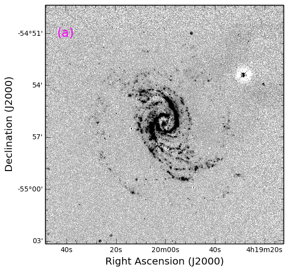
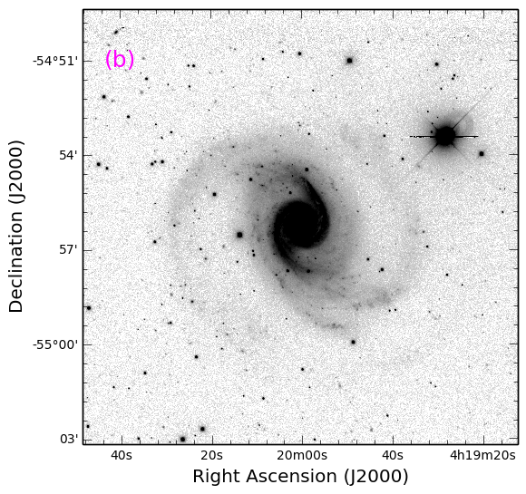
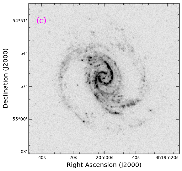
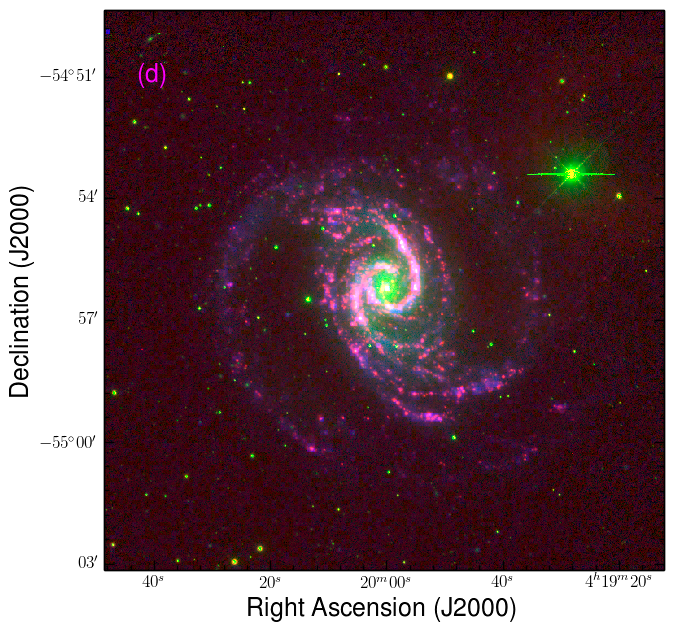
Figure 1: Panel (a) & (b): The SINGG H$\alpha$ and $R$-band image of NGC 1566. Panel (c): The GALEX FUV image of NGC 1566. Panel (d): The three-color RGB image of NGC 1566; Red represents the H$\alpha$ image, Green the $R$-band image and Blue the FUV image. The H$\alpha$, and $R$-band images are convolved to $6^{\prime\prime}$, to match the resolution of the FUV image (Wong, 2007; Meurer et al., 2006).

The formation and evolution of a galaxy is strongly connected to its interactions with the surrounding local environment (Gavazzi & Jaffe, 1986; Okamoto & Habe, 1999; Barnes & Hernquist, 1991; Antonuccio-Delogu et al., 2002; Balogh et al., 2004; Avila-Reese et al., 2005; Blanton et al., 2005; Hahn et al., 2007; Fakhouri & Ma, 2009; Cibinel et al., 2013; Chen et al., 2017; Zheng et al., 2017). The term environment is broad and not only refers to the neighbouring galaxies but also to the tenuous gas and other material between these systems, the so-called intergalactic medium (IGM). These interactions include gas accretion (Larson, 1972; Larson et al., 1980; Tosi, 1988; Sancisi et al., 2008; de Blok et al., 2014b; Vulcani et al., 2018; Rahmani et al., 2018), ram pressure stripping due to the interaction with the IGM (Dickey & Gavazzi, 1991; Balsara et al., 1994; Abadi et al., 1999; Boselli & Gavazzi, 2006; Westmeier et al., 2011; Yoon et al., 2017; Jaffé et al., 2018; Ramos-Martínez et al., 2018), or mergers and tidal harassments (Toomre & Toomre, 1972; Farouki & Shapiro, 1982; Dubinski et al., 1996; Alonso-Herrero et al., 2000; Alonso et al., 2004; Brandl et al., 2009; Blanton & Moustakas, 2009; Moreno et al., 2015; Lagos et al., 2018; Elagali et al., 2018a; Elagali et al., 2018b). There is a plethora of observational evidence on the relationship between galaxies and their local surrounding environment. For instance, the morphology-density relationship (Oemler, 1974; Dressler, 1980; Dressler et al., 1997; Postman et al., 2005; Fogarty et al., 2014; Houghton, 2015), according to which early-type galaxies (ellipticals and lenticulars) are preferentially located in dense environments such as massive groups and clusters of galaxies, whereas late-type galaxies (spirals, irregulars and/or dwarf irregulars) are located in less dense environments, e.g., loose groups and voids. Furthermore, galaxies in dense environments are commonly Hi deficient in comparison with their field counterparts (Davies & Lewis, 1973; Haynes & Giovanelli, 1986; Magri et al., 1988; Cayatte et al., 1990; Quilis et al., 2000; Schröder et al., 2001; Solanes et al., 2001; Omar & Dwarakanath, 2005; Sengupta & Balasubramanyam, 2006; Sengupta et al., 2007; Kilborn et al., 2009; Chung et al., 2009; Cortese et al., 2011; Dénes et al., 2016; Yoon et al., 2017; Brown et al., 2017; Jung et al., 2018). This is because dense environments promote all sorts of galaxy-galaxy and/or galaxy-IGM interactions, which have various consequences on the participant galaxies including their colour and luminosity (Loveday et al., 1992; Norberg et al., 2001; Croton et al., 2005; Kreckel et al., 2012; McNaught-Roberts et al., 2014) as well as their star formation rates (Balogh et al., 1997; Poggianti et al., 1999; Lewis et al., 2002; Gómez et al., 2003; Kauffmann et al., 2004; Porter et al., 2008; Paulino-Afonso et al., 2018; Xie et al., 2018). Hence, a complete picture of the local environments surrounding galaxies is essential to distinguish between the different mechanisms that enable galaxies to grow, or quench (Thomas et al., 2010; Peng et al., 2010; Putman et al., 2012; Marasco et al., 2016; Bahé et al., 2019).

The effects of galaxy interactions with the surrounding environment are most noticeable in the outer discs of the participant galaxies. However, Hi discs are better tracers of the interactions with the local environment, because Hi discs are commonly more extended and diffuse than the optical discs and, as a consequence, more sensitive to external influences and susceptible to hydrodynamic processes unlike stars (Yun et al., 1994; Braun & Thilker, 2004; Michel-Dansac et al., 2010). Probing the faint Hi gaseous structures in galaxies is an onerous endeavour as it requires high observational sensitivity to low surface brightness features, which means long integration times. Such observations are now possible on unprecedentedly large areas of the sky. These wide field Hi surveys will be conducted using state-of-the-art radio telescopes that have subarcminute angular resolution, for instance the Australian Square Kilometre Array Pathfinder (ASKAP; Johnston et al., 2007, 2008), the Karoo Array Telescope (MeerKAT; Jonas & MeerKAT Team, 2016) as well as the APERture Tile In Focus (APERTIF; Verheijen et al., 2008).

The Widefield ASKAP L-band Legacy All-sky Blind surveY (WALLABY) is an Hi imaging survey that will be carried out using ASKAP radio telescope to image $3/4$ of the sky out to a redshift of $z\sim 0.26$ (Koribalski, 2012). ASKAP is equipped with phased-array feeds (PAFs, Hay & O’Sullivan, 2008), which can deliver a field-of-view of $30\,$ square degrees, formed using $36$ beams at $1.4\,$GHz (Koribalski, 2012). WALLABY will provide Hi line cubes with relatively high sensitivity to diffuse emission with a root-mean-square (rms) noise of $1.7\,$mJy beam^-1 per $4$ km s^-1 channel and will map at least $500,000$ Hi emitting galaxies over its entire volume (Duffy et al., 2012). Hence, WALLABY will help revolutionise our understanding of the behaviour of the Hi gas in different environments and the distribution of gas-rich galaxies in their local environments. The prime goal of this work is to provide the community with an example of the capabilities of the widefield Hi spectral line imaging of ASKAP and the scope of the science questions that will be addressable with WALLABY. We present the ASKAP Hi line observations of the spiral galaxy NGC 1566 (also known as WALLABY J041957-545613) and validate these with archival single-dish and interferometric Hi observations from the Parkes $64\,$m telescope using the $21$-cm multibeam receiver (Staveley-Smith et al., 1996) and the Australia Telescope Compact Array (ATCA), respectively. Further, we use the sensitivity and angular resolution of the ASKAP Hi observations to study the asymmetric/lopsided Hi gas morphology and warped disc of NGC 1566 and attempt to disentangle the different environmental processes affecting the gas and the kinematics of this spectacular system. NGC 1566 is a face-on SAB(s)bc spiral galaxy (de Vaucouleurs, 1973; de Vaucouleurs et al., 1976), and is part of the Dorado loose galaxy group (Bajaja et al., 1995; Agüero et al., 2004; Kilborn et al., 2005).

Table 1: The properties of NGC 1566 adopted from the literature and reported in this paper.

Property	NGC 1566	Reference
Right ascension (J2000)	04:20:00.42	de Vaucouleurs (1973)
Declination (J2000)	$-$54:56:16.1	de Vaucouleurs (1973)
Morphology	SAB(rs)bc	de Vaucouleurs (1973)
Hi systemic velocity (km s-1)	$1496$	This work
$L_{\text{R}}$ (L⊙)	$1.2\times 10^{11}$	Meurer et al. (2006)
$L_{\text{FIR}}$ (L⊙)	$2.5\times 10^{10}$	Sanders et al. (2003)
$\mu_{R}$ (ABmag arcsec-2)	$19.3$	Meurer et al. (2006)
$\text{m}_{I}$ (ABmag)	$8.7$	Walsh (1997)
$\text{m}_{3.6\mu m}$ (ABmag)	$10.15$	Laine et al. (2014)
$\text{m}_{V}$ (ABmag)	$9.8$	Walsh (1997)
M∗ (M⊙)	$6.5\times 10^{10}$	This work
H$\alpha$ Equivalent width (Å)	$39\pm 3$	Meurer et al. (2006)
M${}_{\text{FUV}}$ (ABmag)	$-20.66$	Wong (2007)
M${}_{\text{H{\sc{i}}}}$ (M⊙)	$1.94\times 10^{10}$	This work
M${}_{\text{H2}}$ (M⊙)	$1.3\times 10^{9}$	Bajaja et al. (1995)
M${}_{\text{BH}}$ (M⊙)	$8.3\times 10^{6}$	Woo & Urry (2002)
Position angle (degree)	$219\pm 4$	This work
Inclination (degree)	$31\pm 7$	This work
SFR${}_{\text{H}\alpha}$(M⊙ yr-1)	$21.5$	Meurer et al. (2006)
D25 (kpc)	$35$	Walsh (1997)
Distance (Mpc)	$21.3$	Kilborn et al. (2005)

Figure 1 shows the Survey for Ionisation in Neutral Gas Galaxies (SINGG; Meurer et al., 2006) H$\alpha$ and $R$-band images, the GALEX FUV image and a three-color RGB image of NGC 1566, where the H$\alpha$, $R$-band, and FUV images present the Red, Green and the Blue, respectively. This galaxy has a weak central bar (north-south orientation with a length of $\sim 32^{\prime\prime}.5$, Hackwell & Schweizer, 1983) and two prominent star-forming spiral arms that form a pseudo-ring in the outskirts of the optical disc (Comte & Duquennoy, 1982). The H$\alpha$ emission map of NGC 1566 is dominated by a small but extremely bright H$\alpha$ complex region located in the northern arm that emits approximately a quarter of the total disc’s H$\alpha$ flux when excluding the emission from the nucleus (Pence et al., 1990). NGC 1566 hosts a low-luminosity Seyfert nucleus (Reunanen et al., 2002; Levenson et al., 2009; Combes et al., 2014; da Silva et al., 2017) known for its variability from the X-rays to IR bands (Alloin et al., 1986; Glass, 2004). The origin of the variability in AGNs is still controversial and is hypothesised to be caused by processes such as accretion prompted by disc instabilities, surface temperature fluctuations, or even variable heating from coronal X-rays (Abramowicz et al., 1986; Rokaki et al., 1993; Zuo et al., 2012; Ruan et al., 2014; Kozłowski et al., 2016). Although, NGC 1566 has been subjected to numerous detailed multiwavelength studies, as cited above, this work presents the first detailed Hi study of this spiral galaxy. Table 1 presents a summary of the relevant properties of NGC 1566 from the literature and from this paper.

	Table 2. WALLABY early science observations: Dorado field
Observation Dates	Time on Source (hrs)	Bandwidth (MHz)	Central Frequency (MHz)	Number of Antennas	Footprint
28 Dec 2016	11.1			10	A
29 Dec 2016	11.2			10	B
30 Dec 2016	11.1			9	A
31 Dec 2016	12.6	192	1344.5	10	B
01 Jan 2017	11.1			10	A
02 Jan 2017	12.0			10	B
03 Jan 2017	3.8			9	A
23 Sep 2017	12.0			12	A
24 Sep 2017	12.0	240	1368.5	12	B
25 Sep 2017	4.0			12	A
26 Sep 2017	12.0			12	B
27 Sep 2017	12.0			12	A
28 Sep 2017	12.0			12	B
15 Dec 2017	9.1	240	1320.5	16	A
03 Jan 2018	12.0			16	B
04 Jan 2018	9.0			16	A

This paper is organised as follows: in Section 2, we describe the WALLABY early science observations and reduction procedures along with the previously unpublished archival data obtained from the ATCA online archive. Section 3 describes our main results, in which we provide detailed analysis of the Hi morphology and kinematics of this galaxy. In Section 4, we fit the observed rotation curve to three different dark matter halo models, namely, the pseudo-isothermal, the Burkert and the Navarro-Frenk-White (NFW) halo profiles. Section 5 discusses the possible scenarios leading to the asymmetry in the outer gaseous disc of NGC 1566 and presents evidence that ram pressure could be the main cause of this asymmetry. In Section 6, we summarise our main findings. For consistency with previous Hi and X-ray studies of the NGC 1566 galaxy group, we adopt a distance of $21.3\,$Mpc (Kilborn et al., 2005; Osmond & Ponman, 2004), which is based on a Hubble constant of $H_{0}\,=\,70.3\,$km s^-1 Mpc^-1, though we note that this is at the upper end of values quoted in the NASA/IPAC Extragalactic Database (NED). For more details refer to Section 4.5.

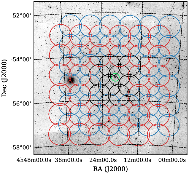
Figure 2: The Dorado observations footprint, where blue and red circles represent footprints A and B, respectively. The inner eight black circles represent the beams around NGC 1566 used in this paper. The background image is the blue band Digitised Sky Survey (DSS) image, and the green circle highlights the location of NGC 1566.

2 Data

2.1 WALLABY Early Science Observations

ASKAP is situated in the Murchison Radioastronomy Observatory in Western Australia, a remote radio-quiet region about $305\,$km North-East of Geraldton in Western Australia. ASKAP is one of the new generation of radio telescopes designed to pave the way for the Square Kilometre Array (SKA; Dewdney et al., 2009). This SKA precursor consists of $36$ separate $12$-metre radio dishes that are located at longitude $116.5^{\circ}$ east and latitude $26.7^{\circ}$ south. Each 12-metre antenna has a single reflector on an azimuth-elevation drive along with a third axis (roll-axis) to provide all-sky coverage and an antenna surface capable of operation up to $10\,$GHz. The antennas are equipped with Mark two (MK ii) phased array feeds (PAFs), which provide the antennas with a $30$ square degree field-of-view, making this radio telescope a surveying machine (DeBoer et al., 2009; Schinckel & Bock, 2016). During the first five years of operation, ASKAP will mainly carry out observations for ten science projects, one of which is WALLABY.

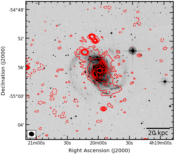
Figure 3: Optical DSS image (blue band) on a linear stretch with contours from ASKAP continuum map overlaid at $-2,2,5,10,15,20,25$ multiplied by $1\,\sigma$ ($0.3\,$mJy beam^-1). The $-2\,\sigma$ level is displayed with dashed contours. The restored beam of ASKAP observation is in the bottom left.

In October 2016, ASKAP early science observations program started using $12$ PAF-equipped ASKAP antennas (out of $36$ antennas) to pave the way and improve the data reduction and analysis techniques while commissioning ASKAP to full specifications. Over $700\,$ hours of early science observations were dedicated to WALLABY, during which four fields were observed to the full survey sensitivity depth, rms noise sensitivity per $4$ km s^-1 channel of $1.7\,$mJy beam^-1 (Lee-Waddell et al., 2019; Reynolds et al., 2019). One of these fields is the Dorado early science field. Figure 2 shows the two interleaves of the square $6\times 6$ beam footprint of the observations overlaid on the Digitised Sky Survey (DSS) image of this field. The blue and red beams are referred to as footprint A (centred at$\,\alpha\,=\,04$:$18$:$35$,$\,\delta\,=\,-54$:$51$:$43\,$; J$2000$) and B (centred at$\,\alpha\,=\,04$:$21$:$44.7$,$\,\delta\,=\,-55$:$18$:$33.8\,$; J$2000$), respectively. Mosaicking the two interleaves reduces the noise level at the edge of the beams and produces a smoother noise pattern. The inner eight black circles represent the beams around NGC 1566 used to make the Hi cube that forms the basis of this work. The green circle shows the location of NGC 1566. The observations of this field started in December $2016$ and were completed in January 2018 using at the beginning only $9\,$-$\,10$ ASKAP antennas, however the most recent observations were completed using $16$ ASKAP antennas. The baseline range of the ASKAP array for the current observations is between $22$-$2305\,$m, which ensured excellent uv-coverage and a compromise between the angular resolution and the surface brightness sensitivity of the observations. The bandwidth of the Dorado observations ranges between $192$ and $240\,$MHz, due to upgrades to the correlator capacity during the early science period, and has a channel width of $18.5\,$kHz ($4\,$km s^-1). For each day of observation, the primary calibrator, PKS1934-638, is observed at the beginning for two to three hours and is positioned at the centre of each of the $36$ beams. The total on-source integration time is $167.0\,$hr; $83.2\,$hr for footprint A and $83.8\,$hr for footprint B. Refer to Table 2 for a summary of the Dorado early science observations.

	Table 3. ASKAP and ATCA Hi Observations Results
Parameter	ASKAP value	ATCA value
rms noise (Jy beam-1 per $4\,$km s-1 channel )	$1.7\times 10^{-3}$	$2.4\times 10^{-3}$
Synthesised Beam Size (arcsec$\times$arcsec)	$42\times 35$	$45\times 40$
Synthesised Beam Size (kpc$\times$kpc)	$4.3\times 3.6$	$4.6\times 4.1$
Beam PA (degree)	$80.0$	$6$
Channel width (km s-1)	$4$	$4$
Channel map pixel size (arcsec$\times$arcsec)	$6\times 6$	$6\times 6$
NGC 1566 Hi total flux (Jy km s-1)	$180.2\pm 16.3$	$177.0\pm 14.0$
NGC 1566 peak flux density (Jy)	$1.35\pm 0.09$	$1.24\pm 0.02$
NGC 1566 Hi mass (M⊙)	$(1.94\pm 0.18)\times 10^{10}$	$(1.91\pm 0.15)\times 10^{10}$
$w_{50}$ Line Width (km s-1)	$208\pm 10$	$201\pm 8$

We use ASKAPSOFT to process the Dorado observations. ASKAPSOFT is a software processing pipeline developed by the ASKAP computing team to do the calibration, spectral line and continuum imaging, as well as the source detection for the full-scale ASKAP observations in a high-performance computing environment. This pipeline is written using C++ and built on the casacore library among other third party libraries. A comprehensive description of ASKAPsoft reduction pipeline is under preparation in Kleiner et al. (in prep.). The reader can also refer to Lee-Waddell et al. (2019) or Reynolds et al. (2019) for a similar brief description of the reduction and pipeline procedures. For each day of observation, we flag and calibrate the measurement data set on a per-beam basis using ASKAPSOFT tasks cflag and cbpcalibrator, respectively. Using the cflag utility, we flag the autocorrelations and the spectral channels affected by radio frequency interference (RFI) by applying a simple flat amplitude threshold. Then, we apply a sequence of Stokes-V flagging and dynamic flagging of amplitudes, integrating over individual spectra. We process the central $8$ beams ($4$ in each footprint) of each observation using an $8\,$MHz bandwidth ($432\,$channels), between $1410$ to $1418\,$MHz (velocity range between $511$ to $2196$ km s^-1) to save computing time and disc space on the Pawsey supercomputer. We then process the calibrated visibilities to make the continuum images using the task imager and self-calibrate (three loops) to remove any artefacts or sidelobes from the continuum images.

	Table 4. Archival ATCA Hi Observations: Instrumental Parameters
Parameter	Array Configuration
	375B	1.5D	750B	1.5C
Observation Dates	1994 April 05	1994 May 26	1994 June 01	1994 June 17
On-source integration time (hrs)	9	9	9	9
Shortest Baseline (m)	31	107	61	77
Longest Baseline (m)	5969	4439	4500	4500
Central Frequency (MHz)	1413	1413	1413	1413
Bandwidth (MHz)	8	8	8	8

Prior to the spectral-line imaging stage, we subtract radio continuum emission from the visibility data set using the best-fit continuum sky model produced in the previous step. Thereafter, we combine the data set for each beam, seven nights in footprint B and nine nights in footprint A, in the uv domain and image using the ASKAPSOFT task imager with a robust weighting value of $+0.5$ and a $30$ arcsec Gaussian taper. We clean the combined image for each beam using a major and minor cycle threshold of $3\sigma$, three times the theoretical rms noise for the seven observations combined. To measure the theoretical rms noise of each epoch, we use the on-line sensitivity calculator , with antenna efficiency value of $0.7$ and system temperature of $50\,$K. For instance, the theoretical rms noise for ten hours using $10$, $12$ or $16$ antennas is $5.03,4.15$ and $3.08\,$mJy beam^-1, respectively. Then, we subtract the residual continuum emission from the restored cube using the ASKAPSOFT task imcontsub and mosaicked the $8$ beams using the ASKAPSOFT task linmos. Even though mosaicking different ASKAP beams with linmos can introduce correlated noise to the final Hi cube, this has no effect on the final flux scale, and only a minor effect on the rms noise. This image domain continuum subtraction is necessary to obtain a higher dynamic range Hi cube and remove any remaining residual artefacts, which aids source finding and parameterisation. Figure 3 shows the optical DSS image (blue band) overlaid with contours from the ASKAP continuum map. The total $21\,$cm continuum flux density of NGC 1566 from ASKAP observations is $199\pm 3\,$mJy, in agreement with the value of $204\pm 28\,$mJy (at $21.7\,$cm ) reported by Ehle et al. (1996) using the ATCA. The restored synthesised beam has a size of $\theta_{\text{FWHM}}\,=\,42^{\prime\prime}\times 35^{\prime\prime}$ with a position angle of $\,80^{\circ}$. The Hi line cube has rms noise per $4\,$km s^-1 channel of $1.7$ mJy beam^-1, which translates to a $3\sigma$ column density sensitivity of $N_{\text{H{\sc{i}}}}\,=\,1.5\times 10^{19}\,$cm^-2. The rms noise in a wider channel width ($20\,$km s^-1) equals $0.84$ mJy beam^-1, and corresponds to a $3\sigma$ column density sensitivity of $N_{\text{H{\sc{i}}}}\,=\,3.7\times 10^{19}\,$cm^-2. The properties of the final cube are summarised in Table 3.

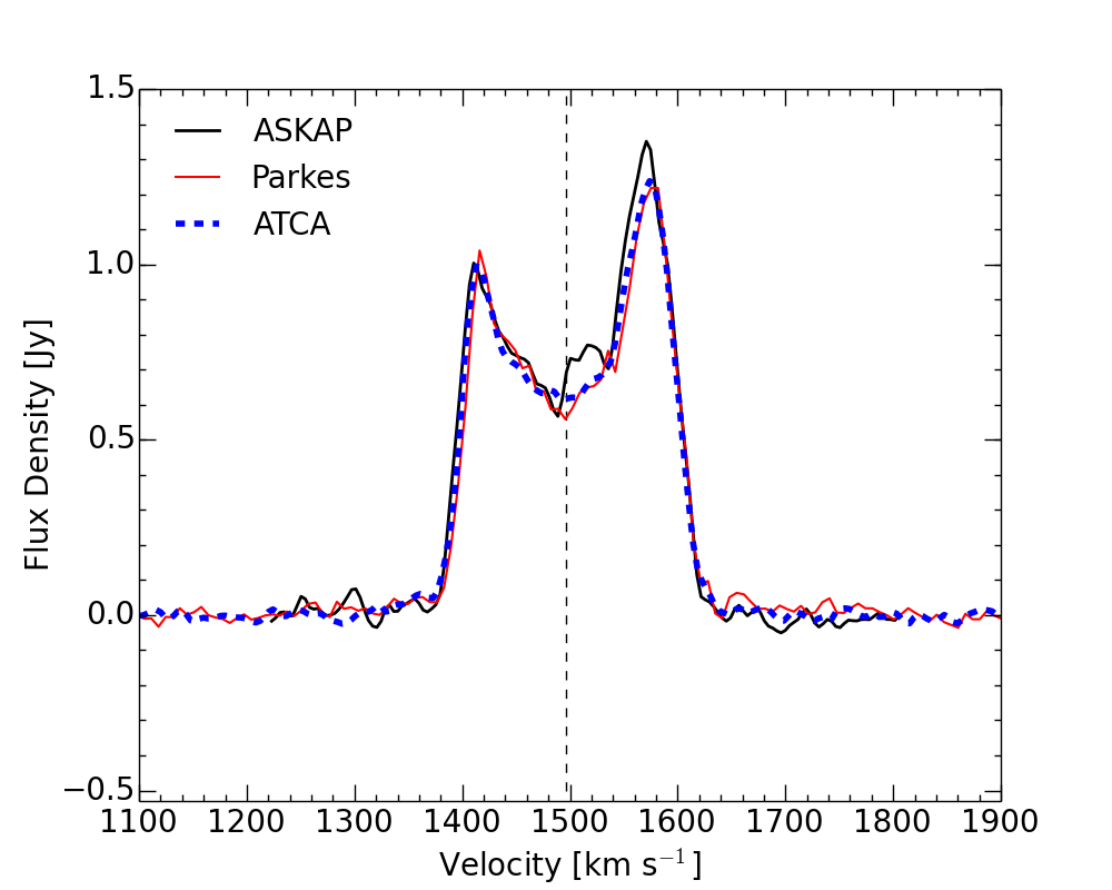
Figure 4: The Hi line profile of NGC 1566 from our ASKAP observations (black line), from the ATCA (blue dashed line) and Parkes single-dish observations (red line). The vertical line delimits the Hi systemic velocity of NGC 1566 $V_{\text{sys}}\,=\,1496\,$km s^-1 derived from our kinematics analysis (refer to Section 3).

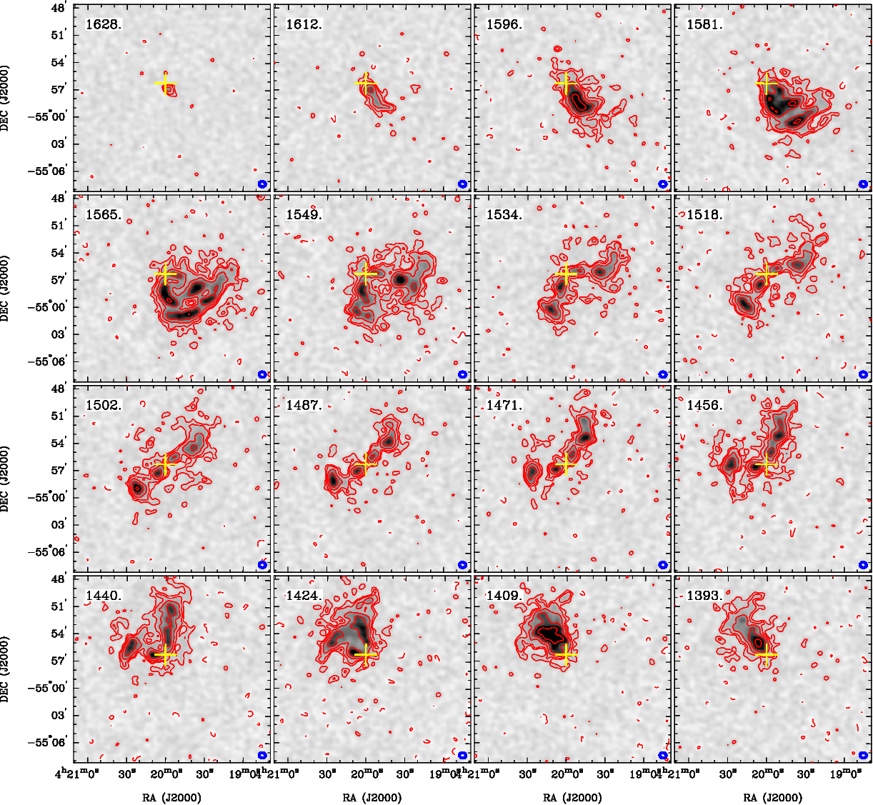
Figure 5: The individual Hi channel maps of NGC 1566 from ASKAP observations in the velocity range between $1628$-$1393\,$km s^-1 and with a step-size of $16\,$km s^-1. The velocity of each channel is shown in the top-left, whereas the restored beam is shown in the bottom-right (blue ellipse). Contours are at $-3,3,5,10,20,40\,$ times the $1\,\sigma$ noise ($0.85\,$ mJy beam^-1 per $16\,$km s^-1 channel). The yellow cross marks the kinematic centre of NGC 1566 derived using rotcur (refer to Section 3).

2.2 ATCA Observations

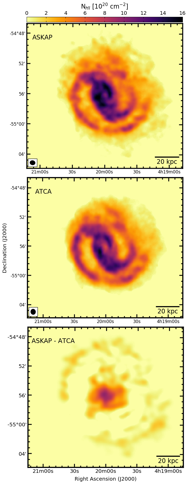
Figure 6: The Hi column density map of NGC 1566 as obtained from ASKAP observations (top panel), the archival ATCA observations (middle panel), and a difference between the two maps (bottom panel). To produce the difference map, we have convolved the ASKAP and ATCA maps to the same beam angular resolution. The ellipse shows the restored beam of ASKAP observations ($\theta_{\text{FWHM}}\,=\,42^{\prime\prime}\times 35^{\prime\prime}$) and the ATCA observations ($\theta_{\text{FWHM}}\,=\,45^{\prime\prime}\times 40^{\prime\prime}$).

NGC 1566 was observed using the ATCA in four epochs between April 1994 and June 1994 with each epoch being $12\,$h in duration. Four different ATCA array configurations were used to observe NGC 1566, namely the 1.5C, 375, 750B as well as the 1.5D configuration (Walsh, 1997). These configurations have baseline distances in the range between $31$ and $5969\,$m. In each of the four epochs, the observation was centred at $1413\,$MHz (the redshifted $1420\,$MHz line frequency for NGC 1566) for a duration of nine hours on the source (a total of $36\,$hrs, see Table 4). The bandwidth of these observations is $8\,$MHz, over $512$ velocity channels. Hence, each channel corresponds to $15.625\,$kHz in width, and a $3.3\,$km s^-1 velocity resolution. The ATCA primary calibrator, PKS1934$-$638 (flux density $S_{\text{1396 MHz}}=14.9\,$Jy), was observed before each epoch of observations for a duration of $30\,$minutes and used as the bandpass calibrator. The phase calibrator PKS0438$-$436 ($S_{\text{1396 MHz}}=6.09\,$Jy) was observed each hour during the four epochs for a duration of $15$ minutes to ensure the precision of the calibration.

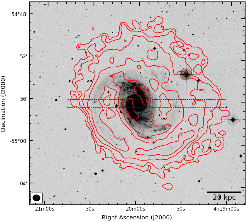
Figure 7: DSS blue band image of NGC 1566 with column density contours from ASKAP observations overlaid at $(0.6,1.2,2.4,4.8,9.6,14.0,16.2)\times 10^{20}\,$cm^-2. The ellipse shows the restored beam of ASKAP observations. Left-to-right in the figure corresponds to east-to-west of the galaxy. The blue-dashed line corresponds to the rectangular cut through the galaxy, with a width of $5\,$kpc, that is used to measure the cut in the column density distribution across NGC 1566 in Figure 8.

We follow the standard procedures described in Elagali et al. (2018a) to flag, calibrate and image the Hi line observations using the miriad package (Sault et al., 1995). We use the miriad uvlin task (Sault, 1994; Cornwell et al., 1992) to subtract the radio continuum from the visibility data set. Then, we use miriad invert task to Fourier-transform the continuum subtracted visibilities to a map with robust weighting parameter of $+0.5$ and a symmetric taper of $15$ arcsec to have an optimal sidelobe suppression and intermediate weighting between uniform and natural. We also re-sample to the ASKAP resolution of $4\,$km s^-1 at this stage, and apply the clean task down to three times the theoretical rms noise. As a final step, we apply the primary beam correction using the linmos task. The synthesised beam-size is $\theta_{\,\text{FWHM}}=45^{\prime\prime}\times 40^{\prime\prime}$ with PA$\,=\,6^{\circ}$. The cube has rms noise per $4\,$km s^-1 channel of $2.4\,$mJy beam^-1, close to the theoretical rms noise of our observations ($2.2\,$mJy beam^-1). The $3\sigma$ column density sensitivity per $4\,$km s^-1 channel is $N_{\text{H{\sc{i}}}}\,=\,1.7\times 10^{19}\,$cm^-2. Over a $20\,$km s^-1 channel width the rms noise equals $1.2$ mJy beam^-1 and the corresponding $3\sigma$ column density sensitivity is $N_{\text{H{\sc{i}}}}\,=\,4.3\times 10^{19}\,$cm^-2.

3 Gas Morphology and Kinematics

3.1 Hi Morphology and distribution in NGC 1566

Figure 4 presents the integrated Hi spectrum of NGC 1566 as obtained from ASKAP observations (black line), unpublished archival ATCA observations (blue dashed-line) and re-measured Parkes single-dish spectrum (red line) from Kilborn et al. (2005). We measure a total flux value of $180.2\pm 16.3\,$Jy km s^-1 from ASKAP observations. This flux value corresponds to a total Hi mass of $1.94\times 10^{10}\,$M_⊙, assuming that NGC 1566 is at a distance of $21.3\,$Mpc. The integrated Hi flux density of NGC 1566 from ASKAP early science observations is within the expected error of the value measured from the ATCA observations ($177.0\pm 14.0\,$Jy km s^-1) and from Parkes observations ($175.0\pm 7.4\,$Jy km s^-1). We note that the integrated flux density of NGC 1566 derived from our ATCA data reduction is within error of the value reported in the thesis of Walsh (1997). Figure 5 presents the individual Hi channel maps of NGC 1566 from ASKAP observations in the velocity range between $1628$-$1393\,$km s^-1 and with a step-size of $16\,$km s^-1. Figure 6 shows the Hi column density map of NGC 1566 as obtained from ASKAP observations (top panel), the archival ATCA observations (middle panel), and a difference between the two maps (bottom panel). To produce the difference map, we have convolved the ASKAP and ATCA maps to the same beam angular resolution. ASKAP observations are as sensitive as the ATCA observations to low surface brightness features surrounding the outer disc of NGC 1566. This figure emphasises the ability of the ASKAP instrument to probe relatively low column density levels while mapping large areas of the sky. The small flux difference between ASKAP and ATCA in the centre is likely due to the smaller baseline of the ASKAP configuration in comparison with that of the ATCA, however this difference is within the error of the two instruments. Hence, ASKAP will provide the Hi community with unprecedented amount of high quality Hi line cubes. We note that Reeves et al. (2016) presented the moment zero and velocity maps of NGC 1566 using more recent ATCA observations but with less integration time ($\sim 17\,$hrs) in comparison with the archival ATCA data used in this paper ($\sim 36\,$hrs). The study of Reeves et al. (2016) was mainly focused on the intervening Hi absorption in NGC 1566 along with other nine nearby galaxies.

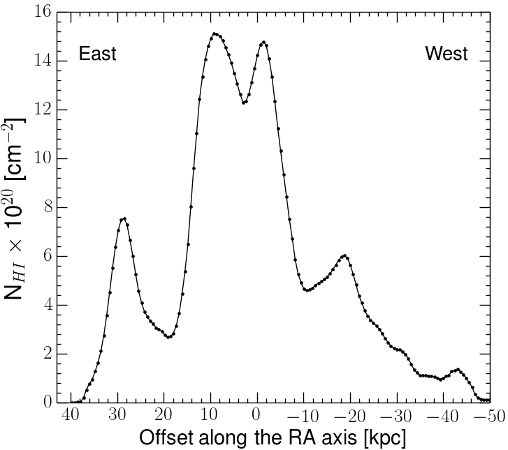
Figure 8: A column density cut across NGC 1566 with respect to right ascension offset from the centre of the galaxy. The width of this cut is $5\,$kpc and is shown by the blue-dashed line in Figure 7. Left-to-right in the figure corresponds to east-to-west.

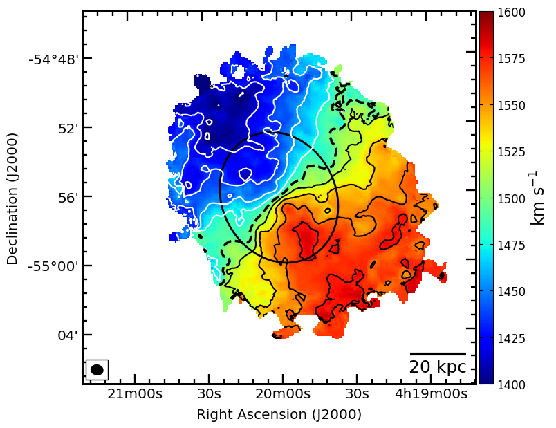
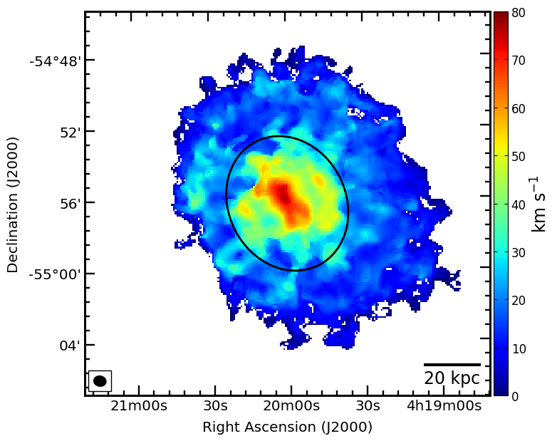
Figure 9: The ASKAP line-of-sight velocity (left) and velocity dispersion (right) of NGC 1566. The ellipse marks the optical disc of NGC 1566 (Walsh, 1997). Contours are centred at the systemic velocity of NGC 1566 ($1496\,$km s^-1; black-dashed contour) and are equally separated by $20\,$km s^-1 interval; white and black contours show the approaching and receding sides, respectively. The black filled ellipse shows the restored beam of the observations.

Figure 7 shows the optical DSS blue band image of NGC 1566 with column density contours from ASKAP observations overlaid at $(0.6,1.2,2.4,4.8,9.6,14.0,16.2)\times 10^{20}\,$cm^-2. This map shows an Hi disc that extends beyond the observed optical disc especially around the northern and western parts of NGC 1566 (also refer to Figure 15). The Hi gas is very concentrated in the inner arms and gradually decreases following the outer arms of the disc. The Hi also highlights the difference between the two outer arms better than in the optical (Figure 1). The eastern outer arm forms a regular arc shape that extends between PA$\,=50^{\circ}$ until where the PA$\,=\,260^{\circ}$; here the PA is estimated from the north extending eastwards to the receding side of the major axis. However, the western arm is significantly shorter extending from PA$\,=\,210^{\circ}$ to PA$\,=\,330^{\circ}$, and appears less regular or disturbed between PA$\,=\,270^{\circ}$ to $330^{\circ}$. The $1.5\times 10^{19}\,$cm^-2 column density contour extends for a diameter of almost $16^{\prime}$, which at the adopted distance of NGC 1566 translates to a diameter of $\sim 99\,$kpc. Figure 8 shows a column density cut across NGC 1566 with respect to right ascension offset from the centre and measured at the declination of the centre of the galaxy. The width of this cut is $5\,$kpc and is shown by the blue-dashed line in Figure 7. We use the karma visualisation tool kvis to generate this column density cut across NGC 1566 (Gooch, 1996). The column density of the Hi gas slowly drops with radius, mainly due to presence of the outer arms in NGC 1566 at radius $r\,\sim 20$kpc; the column density falls off at $r\,\sim 20\,$kpc by only a factor of two from the peak value at $r\,\sim 6\,$kpc. Further, Figure 8 shows an asymmetry in the distribution of the Hi gas in this galaxy; the eastern part of the Hi disc sharply declines after $\sim 30\,$kpc from the centre as opposed to the western part which extends beyond $\sim 30\,$kpc and smoothly declines up to a radius of $\sim 50\,$kpc. This asymmetry is more evident in Figure 7, in which the Hi contours show crowding on the east side of the galaxy and are spread out on the west side. The column density asymmetries present in NGC 1566 could be signs of ram pressure interaction, gas accretion and/or past flyby interaction(s) with the other members of NGC 1566 galaxy group. We discuss the possibility of these interaction scenarios in Section 5.

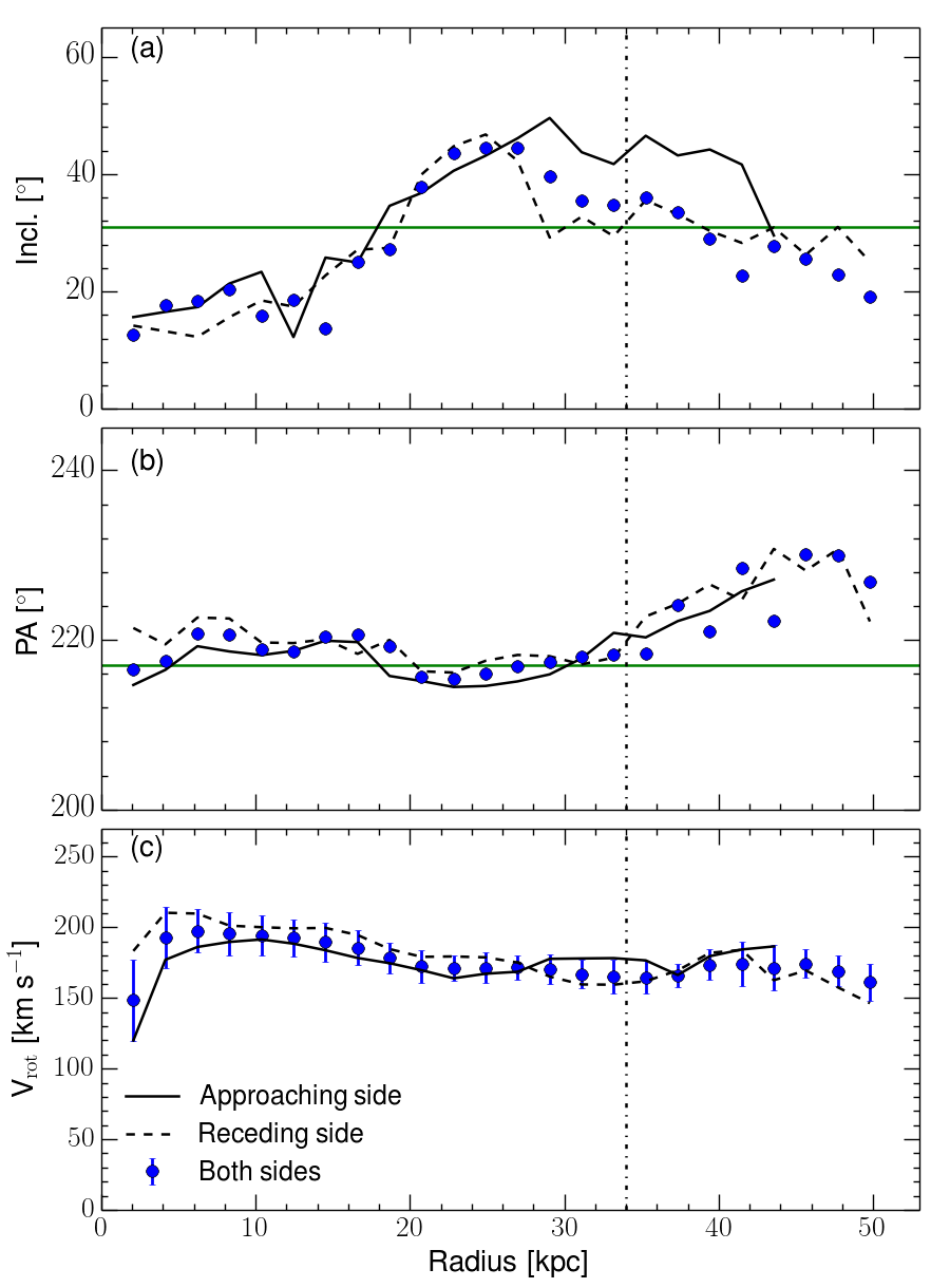
Figure 10: The tilted ring model solutions for the inclination (a), the position angle (b), and the rotation velocity $V_{\text{rot}}$ (c) of NGC 1566 using rotcur. Solid line, dashed line and filled blue circles denote the approaching, receding and both sides, respectively. The green horizontal lines mark the best fit values for the i ($\,31^{\circ}$) and PA ($\,219^{\circ}$), respectively, which are used to estimate the rotation curve for both sides in the panel (c). The vertical dash-dotted line shows the location of the optical radius of NGC 1566 (Walsh, 1997).

3.2 Hi KINEMATICS

Previous studies of the kinematics of NGC 1566 utilised optical spectroscopy to map the numerous emission line regions in this galaxy. For example, Pence et al. (1990) used the Fabry-Pérot interferometer at the $3.9\,$m Anglo-Australian Telescope to map the H$\alpha$ emission in NGC 1566 and were able to measure gas velocities out to a radius of $10\,$kpc (c.f. Figures 4 & 8 in Pence et al., 1990). Figure 9 shows the ASKAP line-of-sight velocity and the velocity dispersion of NGC 1566. The shape of the isovelocity contours of the approaching side (white contours) of the galaxy is slightly different in comparison with the receding side (black contours) which suggests the presence of kinematic asymmetry in NGC 1566. The western side of the velocity field shows significant asymmetry in comparison with the eastern side. This is also seen in both the moment zero map and the velocity channel map in Figures 5 and 6. In the individual channel maps, the western side is more extended than the eastern side, especially at velocities between $1534-1456\,$km s^-1. On the other hand, the dispersion map shows a very high peak in the inner regions which is likely a result of beam smearing. There is a noticeable increase in the velocity dispersion associated with the inner arms of NGC 1566, similar to other grand design spirals like M83 (Heald et al., 2016). However the dispersion velocity decreases quickly in the outer arms and the outskirts of the HI disc. We discuss in detail the possibility of an interaction scenario and other external influences that may lead to the lopsidedness in NGC 1566 in Section 5.

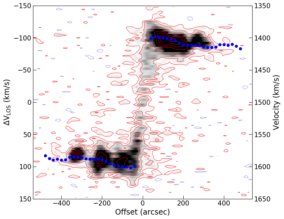
Figure 11: The position-velocity diagram of NGC 1566 along the major axis, overlayed is the rotation curve derived using rotcur. The red contours are at $2,4,8,16,20\,$ times the $1\,\sigma$ noise level ($1.7\,$ mJy beam^-1 per $4\,$km s^-1 channel), while the blue contour is at $-2\,\sigma$.

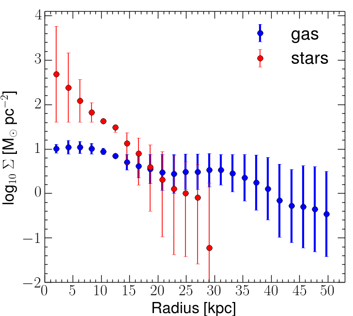
Figure 12: The gaseous and stellar radial mass surface density distributions in NGC 1566 shown in blue and red, respectively.

We follow the standard procedure described in Elagali et al. (2018a) to derive the Hi rotation curve of NGC 1566 using a tilted ring model. This model assumes that the gas moves in circular orbits. Each tilted ring is fitted independently as a function of radius and has $6$ defining kinematic parameters: the central coordinate (x_c,y_c), the systemic velocity $V_{\text{sys}}$, the circular velocity $V_{\text{rot}}$, the inclination angle i, as well as the position angle PA. According to this model, the observed line-of-sight velocity V(x,y) is given by:

$$V(x,y)=V_{\text{sys}}+V_{\text{rot}}\,\sin i\,\text{cos}\,\theta,$$ (1)

where the angle $\theta$ is a function of position angle and inclination. We use the Groningen Image Processing System (gipsy; Allen et al., 1985; van der Hulst et al., 1992) rotcur task (Begeman, 1989) to apply the tilted ring model to the observed velocity fields of NGC 1566. We run the task in an iterative fashion to determine the above mentioned free kinematic parameters for each ring, and use a ring width that equals half the restored beam-size ($\sim 20$ arcsec), i.e., we fit two rings per beam-size. Since the minor axis provides no information on the rotation curve, we apply $|\cos\,\theta|$ weighting function to minimise the contribution of points far from the major axis. Firstly, we fit the systemic velocity $V_{\text{sys}}$ and the dynamical centre out to the edge of the optical disc simultaneously by fixing the PA ($221^{\circ}$) and i ($27^{\circ}$) to their optical values (Pence et al., 1990). We next fit the inclination and position angle simultaneously, keeping the systemic velocity and the dynamical centre fixed to the determined values from the previous step. Then, we smooth the PA and i profiles with a radial boxcar function, estimate their average values and derive an optimum solution for the $V_{\text{rot}}$. The best fit for the systemic velocity of NGC 1566 is $V_{\text{sys}}\,=\,1496\pm 7\,$km s^-1, and the derived dynamical Hi centre agrees with the optical centre. The position angle and inclination values estimated using rotcur are PA$\,=\,219^{\circ}\pm 4^{\circ}$ and i$\,=\,31^{\circ}\pm 7^{\circ}$, respectively, and are within the error of the optical values determined by Pence et al. (1990). We derive the rotation curve for both the receding and approaching sides, to check for possible departures from symmetry and highlight any systematic uncertainties associated with our final results.

Figure 10 shows rotcur results for the inclination, the position angle and the rotation velocity of NGC 1566. The variation of the inclination with radius implies the existence of a mild warp in the Hi disc of this galaxy. The inclination of the inner regions of the disc can be averaged to the value $19^{\circ}$ ($r=<15\,$kpc), while the outer parts of the disc ($r>15\,$kpc) have an average inclination value of $37^{\circ}$. We refer the reader to Figure 19, a 3D interactive visualisation of NGC 1566, the three axes in this visualisation are RA, Dec, and the velocity. On the other hand, the position angle derived using rotcur is constrained across the Hi disc. The green horizontal lines mark the best fit values for the i ($\,31^{\circ}$) and PA ($\,219^{\circ}$), respectively, which are used to estimate the rotation curve for both sides in the lower panel. The rotation of the approaching side is slightly different in comparison with the receding side’s rotation. Figure 11 presents the position-velocity diagram of NGC 1566 along the major axis, with its rotation curve overlaid. We note that the low-level emission apparent in the forbidden quadrants (gas with forbidden velocities) is not real and is due to sidelobes. The rotation of both sides reaches a velocity $V_{\text{rot}}\,=161\pm 13\,$km s^-1 at a radius $r\,=\,50\,$kpc. This velocity translates to, assuming a spherically-symmetric mass distribution, a total dynamical mass of $M_{tot}\,=\,(11.30\pm 1.91$)$\times 10^{11}\,M_{\odot}$ enclosed within this radius. As the fitted inclination of $31^{\circ}$ is outside the typical range where rotcur is thought to be reliable (Begeman, 1989), we also use the the Fully Automated 3D Tilted Ring Fitting Code (FAT; Kamphuis et al., 2015) to derive the rotation curve of NGC 1566. This software works directly on the data cube, thus fitting in 3D, and is more robust against certain instrumental effects and hence is thought to be reliable to lower inclinations (Kamphuis et al., 2015). The results from FAT are consistent with those derived using rotcur. Hence, for brevity, we decide to only show and use the rotcur results.

4 Dark matter content and mass models

The gravitational potential of any galaxy is a function of its combined gaseous, stellar and dark matter mass components. In this section, we investigate the distribution of the dark and baryonic matter in NGC 1566, and fit different mass models to the observed rotation curve of this system using the gipsy task rotmas. rotmas fits the following equation to the observed rotation ($V_{\text{obs}}$):

$$V_{\text{DM}}^{2}(r)=V_{\text{obs}}^{2}(r)-V_{*}^{2}(r)-V_{\text{gas}}^{2}(r),$$ (2)

where $V_{\text{*}}$, $V_{\text{gas}}$, and $V_{\text{DM}}$ are the contributions of the stars, gas and the dark matter components to the total rotation curve of NGC 1566, respectively. The velocity contributions of the gaseous and the stellar mass components are estimated from their mass radial surface density distribution ($\Sigma({r})$) using the gipsy task rotmod (Casertano, 1983). Below, we present the gaseous and the stellar mass radial surface density distributions along with the different dark matter models used to fit the total rotation curve in equation 2.

4.1 Gaseous Distribution

To estimate the gaseous mass surface density profile, we use the Hi column density map obtained from our ASKAP observations (Figure 7). The gas surface density is measured in tilted rings using similar parameters (i, PA, dynamical centre) to those used to derive the total rotation curve with rotcur. We use the task ellint in gipsy to derive the radial Hi column density profile $N_{\text{H{\sc{i}}}}$($r$). We then convert the Hi column density profile to gaseous mass surface density. We scale the gas mass surface density by a factor of $1.4$ to account for the presence of helium and metals and assume that it is optically thin. Figure 12 shows the gas mass surface density profile of NGC 1566. We use the radial gas mass surface density profile of NGC 1566 to estimate the corresponding gas rotation velocities and assume that the gas is mainly distributed in a thin disc.

4.2 Stellar Distribution

To derive the stellar mass surface density profile in NGC 1566, we use the infrared (IR) photometry obtained from the Infrared Array Camera (IRAC) on board the Spitzer Space Telescope (Werner et al., 2004; Fazio et al., 2004). We convert the IR radial flux density distribution ($S_{\lambda}({r})$) to stellar radial mass density distribution ($\Sigma_{*}({r})$) using the following equation:

$$\Sigma_{*}({r})\sim S_{\lambda}({r})Y_{\lambda},$$ (3)

where $\lambda$ indicates the wavelength band and $Y_{\lambda}$ is the mass-to-light ratio with respect to that band. Here, we derive the surface density profile in two different bands, namely, the IRAC $3.6$ and $4.5\,\mu$m bands. We follow the approach in Oh et al. (2008) to derive the mass-to-light ratio of the IRAC two near-infrared bands; for NGC 1566 the values are $Y\,$=$\,0.648\pm 0.073$ and $0.611\pm 0.072$ for the $3.6$ and $4.5\,\mu$m bands, respectively. Similar to the gaseous profile, we use ellint to measure the near-infrared flux density in tilted rings with the same parameters (i, PA, dynamical centre) used to derive the rotation curve of NGC 1566.

We then convert the near-infrared flux density from the IRAC pipeline flux units (MJy sr^-1) to solar units and apply aperture correction for the $3.6$ and $4.5\,\mu$m flux density. The stellar mass radial surface density $\Sigma_{*}({r})$, is calculated by the following equation:

$$\Sigma_{*}({r})=C_{\lambda}Y_{\lambda}f_{\lambda}\frac{S_{\lambda}({r})}{ZP},$$ (4)

where $f_{\lambda}$ is the aperture correction factor, $C_{\lambda}$ is the conversion factor and $ZP$ is the zero point magnitude for each band. We adopt aperture correction values of $f_{3.6\mu\text{m}}\,=\,0.944$ and $f_{4.5\mu\text{m}}\,=\,0.937$ and zero point magnitude fluxes of $280.9$ and $179.7\,$Jy for the $3.6$ and $4.5\,\mu$m (Reach et al., 2005), respectively. Following the calculations in Oh et al. (2008) based on the spectral-energy distributions of the Sun, we use $C_{3.6\mu\text{m}}\,=\,0.196$ and $C_{4.5\mu\text{m}}\,=\,0.201\,$M_⊙pc^-2. Figure 12 shows the stellar mass radial surface density profile of NGC 1566. We measure a total stellar mass of ($6.5\pm 0.4$)$\,\times 10^{10}\,$M_⊙, using the averaged $3.6$ and $4.5\,\mu$m bands stellar mass radial surface density profiles, which is within the error of the value reported in Laine et al. (2014). The stellar mass radial profile can be described by a simple exponential function ($\Sigma_{*}\sim\text{exp}(-r/h)$), for which the the radial scale-length ($h$) equals $\,3\,$kpc and thus the scale-height of the disc ($z_{0}$), using $h/z_{0}\,\simeq\,5\,$(Kregel et al., 2002; van der Kruit & Searle, 1981), equals $0.6\,$kpc. Using rotmod, we construct the stellar velocity component from the stellar mass radial surface density profile of NGC 1566, assuming that the stellar disc has a vertical sech² scale-height distribution with $z_{0}\,=\,0.6\,$kpc (van der Kruit & Searle, 1981).

4.3 Dark Matter Halo Profiles

4.3.1 Pseudo-isothermal Dark matter Profile

This profile is the simplest and most commonly used in the studies of galaxies’ rotation curves (Kent, 1987; Begeman et al., 1991). This model assumes a central constant-density core ($\rho_{0}$ ) and a density profile given by:

$$\rho({r})=\frac{\rho_{0}}{1+(r/r_{c})^{2}},$$ (5)

where $r_{c}$ is the core radius. The corresponding rotation velocity ($v(r)$) to the pseudo-isothermal (ISO) potential is:

$$v^{2}({r})=4\pi G\rho_{0}r_{c}^{2}\Big{[}1-\frac{r_{c}}{r}\arctan\Big{(}\frac{r}{r_{c}}\Big{)}\Big{]},$$ (6)

(Kent, 1986).

4.3.2 Burkert Dark matter Profile

This profile adopts the following definition for the dark matter density profile Burkert (1995):

$$\rho({r})=\frac{\rho_{0}r_{c}^{3}}{(r+r_{c})(r^{2}+r_{c}^{2})},$$ (7)

Similar to the ISO profile, $r_{c}$ and $\rho_{0}$ denote the core radius and the central density of the dark matter halo, respectively. This profile resembles the distribution expected for a pseudo-isothermal sphere at the inner radii ($r<<r_{c}$) and predicts central density $\rho_{0}$. At larger radii, the Burkert density profile $\rho({r})$ is roughly proportional to $r^{-3}$. The velocity corresponding to this profile is given by (Salucci & Burkert, 2000):

$$v^{2}({r})=\frac{6.4G\rho_{0}r_{c}^{3}}{r}\Big{[}\ln\Big{(}1+\frac{r}{r_{c}}\Big{)}+\frac{1}{2}\ln\Big{(}1+\frac{r^{2}}{r_{c}^{2}}\Big{)}-\arctan\Big{(}\frac{r}{r_{c}}\Big{)}\Big{]}.$$ (8)

To fit the rotation curve of this halo profile, we have two free parameters, namely, the core radius and the central density of the dark matter halo.

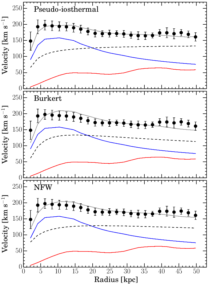
Figure 13: The mass models fit to the observed rotation curve of NGC 1566 using the ISO, Burkert and NFW dark matter profiles. The black circles and grey line show the observed rotation curve and the best fit modelled rotation curve of NGC 1566, respectively. The red, blue and dashed-black lines show the contributions of the gaseous, stellar and dark matter components to the overall rotation curve of NGC 1566, respectively.

4.3.3 NFW Dark matter Profile

Navarro et al. (1996, 1997) used N-body simulations to explore the equilibrium density profile of the dark matter halos in a hierarchically clustering universe and found that these profiles have the same shape, regardless of the values of the cosmological parameters or the initial density fluctuation spectrum. The density profile in this case can be described by the following equation:

$$\rho({r})=\frac{\delta_{c}\rho_{crit}}{\frac{r}{r_{s}}\Big{(}1+\frac{r}{r_{s}}\Big{)}^{2}},$$ (9)

where $r_{\text{s}}$ is the scale radius, $\delta_{c}$ is a critical dimensionless density of the halo and $\rho_{\text{crit}}$ is the critical density for closure. The NFW halo profile is similar to the Burkert profile; the only difference is at $r<<r_{s}$, in which the NFW halo density $\rho({r})\sim r^{-1}$ instead of a constant core density value as it is the case for the Burkert profile. The velocity of this profile is given by:

$$v^{2}({r})=\frac{v_{200}^{2}}{x}\frac{\ln(1+cx)-\frac{cx}{1+cx}}{\ln(1+c)-\frac{c}{1+c}},$$ (10)

where $x$ is the radius ($x\,=\,r$/$r_{200}$) in virial radius units, $c$ is the halo concentration $c\,=\,r_{200}$/$r_{s}$ and $v_{200}$ is the circular velocity at $r_{200}$:

$$v_{200}=\sqrt{\frac{GM_{200}}{r_{200}}}\,=\,10H_{0}r_{200}.$$ (11)

Here, $H_{0}$ is the Hubble constant and $M_{200}$ is the virial mass. To fit the rotation curve of the NFW halo profile, we have two free parameters, namely, the scale radius and the virial radius of the dark matter halo.

4.4 Mass Model Results

To derive the dark matter contribution to the total rotation curve of NGC 1566, we fit equation 2 using rotmas. Figure 13 shows the mass model results using the ISO, Burkert and the NFW halo profiles. Table 6 lists the results of our mass models. In all models, the stellar disc dominates the rotation curve up to a radius $r\sim 18\,$kpc and starts to sharply decline at $r\gtrsim 20\,$kpc. On the other hand the dark matter rises linearly with radius reaching the maximum at $r\sim 10\,$kpc and remains fairly constant at larger radii. Based on the ISO, Burkert and the NFW halo profiles, we estimate dark matter fractions in NGC 1566 to be $\simeq 0.66$, $\simeq 0.58$ and $\simeq 0.62$, respectively. The three dark matter profiles result in reasonable fits. However, due to the lack of angular resolution in the inner regions of NGC 1566 ($\sim 2\,$kpc), we can not differentiate between the three dark matter density profiles. To distinguish between different dark matter halo profiles, higher angular resolution observations of few hundred parsec scales are required (see for example Oh et al., 2015; de Blok, 2010; Bolatto et al., 2002; de Blok et al., 2001). This question will soon be addressable for large samples of nearby galaxies using the $36$ ASKAP antennas (longest baseline of $6\,$km) and MeerKAT telescope (de Blok et al., 2016), which will aid constraining the mass distributions of both the dark and baryonic matter in large numbers of galaxies.

Table 6. Mass models fit results for NGC 1566.
Parameter	Pseudo-isothermal	Burkert	NFW
$r_{\text{c}}$ (kpc)	$1.9\pm 0.6$	$4.3\pm 0.8$	-
$\rho_{\text{0}}$ (M⊙ pc-3)	$0.092\pm 0.050$	$0.082\pm 0.037$	-
$r_{\text{s}}$ (kpc)	-	-	$9.52\pm 1.78$
$r_{\text{200}}$ (kpc)	-	-	$80.84\pm 3.71$
M${}_{\text{DM}}$ ($10^{11}$M⊙)	$7.60$	$5.38$	$6.29$
$\chi_{\text{red}}^{2}$	$0.34$	$1.36$	$0.65$
$f_{\text{DM}}$	$0.66$	$0.58$	$0.62$

4.5 Tully-Fisher Distance of NGC 1566

Here, we use the Tully-Fisher (TF) relation (Tully & Fisher, 1977) in an attempt to measure a more accurate distance for NGC 1566 than currently reported in the literature. We use the $I$-band apparent magnitude ($\text{m}_{I}$) and line width ($w_{50}$) values reported in Table 1 & 3, respectively, and the kinematic inclination derived in Section 3.2. The distance of NGC 1566 using the $I$-band TF relation (Masters et al., 2006) is $16.9^{+7.5}_{-4.1}\,$Mpc, which is smaller than the value we adopt but within the errors. Unfortunately, the error in the TF distance does not allow us to definitively exclude the far distance value reported in NED nor claim a superior distance measurement for this galaxy. We have therefore left the nominal distance of this galaxy as $21.3\,$ Mpc throughout this paper. The large error in the TF relation is due to the low inclination of NGC 1566, which is also reflected by the large uncertainties in the distance measurements for this galaxy in the literature.

5 Discussion

5.1 Possible Origins for the Hi Disc Asymmetries

Many disc galaxies are asymmetric, and have lopsided stellar and/or gaseous components (Baldwin et al., 1980; Bournaud et al., 2005; Mapelli et al., 2008). Both theoretical and observational studies suggest three different environmental mechanisms that can cause such asymmetries, namely, ram pressure interactions with the IGM, galactic interactions as well as gas accretion from hosting/neighbouring filaments (Oosterloo et al., 2007; McConnachie et al., 2007; Reichard et al., 2008; Mapelli et al., 2008; Yozin & Bekki, 2014; de Blok et al., 2014b; Vulcani et al., 2018). In this subsection, we explore the possibility of each of these scenarios given the available data for NGC 1566. Below, we combine the discussion of the galactic interactions and gas accretion scenarios in one subsection for brevity while discussing the ram pressure stripping scenario separately.

5.1.1 Interactions and/or Accretion Scenarios

Tidal interactions between NGC 1566 and neighbouring galaxies could lead to its asymmetries and warps. The interacting galaxy pair NGC 1596/1602 (Chung et al., 2006) is a possible candidate for such a tidal encounter, the physical projected separation between this galaxy pair and NGC 1566 is $\sim 700\,$kpc ($2^{\circ}$ on the sky). Figure 14 shows the column density map of NGC 1566 mosaic field. We detect six galaxies including NGC 1566 in this mosaic. A detailed description of these galaxies and the remainder of the Dorado group galaxies will be presented in Elagali et al. (in prep.) and Rhee et al. (in prep.). Even though tidal interactions between NGC 1566 and the neighbouring galaxies may have occurred, we do not see any Hi tail/bridge that would result from such an interaction. The centre of the NGC 1566 group is shown by the blue filled circle in Figure 14, as defined by where the two most massive and bright galaxies of this group are located, namely NGC 1553/1549 (Kormendy, 1984; Kilborn et al., 2005; Kourkchi & Tully, 2017). We detect no Hi emission above the rms noise of ASKAP observations from this interacting galaxy pair. The upper Hi mass limit of NGC 1553/1549 based on the $3\sigma$ noise level of this observations and over $40\,$km s^-1 channel widths (ten channels) is $\simeq 3.7\times 10^{6}\,$M_⊙ beam^-1 at the distance of this galaxy pair ($17.6\,$Mpc, Kilborn et al., 2005).

Figure 15 presents a deep optical image of NGC 1566 taken by David Malin at the Australian Astronomical Observatory. We also examine this deep image and see no faint stellar substructures around NGC 1566, nor a dramatic system of streams/plumes that may have formed through a tidal interaction or minor merger with neighbouring galaxies; see for example Kado-Fong et al. (2018); Pop et al. (2018); Elagali et al. (2018a); Martínez-Delgado et al. (2015); de Blok et al. (2014a); Martínez-Delgado et al. (2010). We note that these faint structures can form on timescales of $10^{8}$ years and exist for few gigayears after the interaction (Hernquist & Quinn, 1988, 1989). Hence, a recent interaction scenario is less likely to be the reason for the asymmetries seen in the outer Hi disc of NGC 1566. Alternatively, the lopsidedness of the Hi distribution of NGC 1566 can be a result of gas accretion. de Blok et al. (2014b) present an example of this scenario, in which a low column density, extended cloud is connected to the observed main Hi disc of NGC 2403. In the case of NGC 1566, we do not detect any clouds or filaments connected to, or in the nearby vicinity of, the Hi disc of this galaxy. We note that our $3\sigma$ column density sensitivity measured over a $20\,$km s^-1 width is $N_{\text{H{\sc{i}}}}\,=\,3.7\times 10^{19}\,$cm^-2. Therefore, it is difficult to say any more quantitative/conclusive statements about the accretion effects on the Hi disc of NGC 1566 and that more sensitive Hi observations of this galaxy are needed to rule out an accretion scenario.

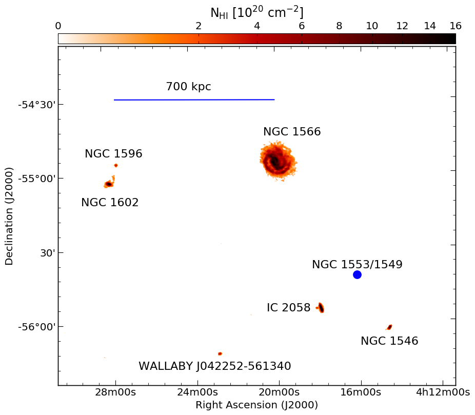
Figure 14: The Hi column density map of NGC 1566 mosaic field as revealed by ASKAP early science observations. The synthesised beam size is $\theta_{\text{FWHM}}\,=\,42^{\prime\prime}\times 35^{\prime\prime}$. There are six galaxies detected in this mosaic, within a velocity range between $950-2040$ km s^-1. The projected physical distance between NGC 1566 and the galaxy pair NGC 1596/1602 is shown by the blue horizontal line. The blue filled circle shows the centre of the group, and the location of the two interacting galaxies NGC 1553/1549 (Kilborn et al., 2005; Kourkchi & Tully, 2017).

5.1.2 Ram Pressure Stripping Scenario

Ram pressure is widely observed in massive galaxy clusters (White et al., 1991; Abadi et al., 1999; Acreman et al., 2003; Randall et al., 2008; Vollmer, 2009; Merluzzi et al., 2016; Ruggiero & Lima Neto, 2017; Sheen et al., 2017), such as the nearby Virgo cluster (Chung et al., 2007; Yoon et al., 2017), and is the main reason for the stripping and removal of gas in galaxy clusters especially closer to their dynamical centres. Even though ram pressure stripping is not as prevalent in galaxy groups, a few cases have been reported in the literature (Kantharia et al., 2005; McConnachie et al., 2007; Westmeier et al., 2011; Rasmussen et al., 2012; Heald et al., 2016; Vulcani et al., 2018). Many authors also ascribe ram pressure as a potential cause for Hi deficiency in groups (see for example Sengupta & Balasubramanyam, 2006; Sengupta et al., 2007; Freeland et al., 2010; Dénes et al., 2016). Here, we investigate the asymmetries present in the outskirts of NGC 1566 and its connection to the gaseous halo undergoing ram pressure stripping as a consequence of its interaction with the IGM. As a galaxy passes through the IGM with an inclined orientation, the Hi gas will be compressed in the leading edge of the outer disc while the gas at the lagging edge get stripped and pulled away as a result of the ram-pressure forces (refer to Figure 1 and 3 in Quilis et al., 2000). This will produce an asymmetry in the Hi column density distribution similar to that observed in NGC 1566, in which the south-eastern edge of the Hi disc sharply declines after $\sim 30\,$kpc from the centre, while the north-western edge is more extended and smoothly declines with radius up to $\sim 50\,$kpc (refer to Figures 7 & 8).

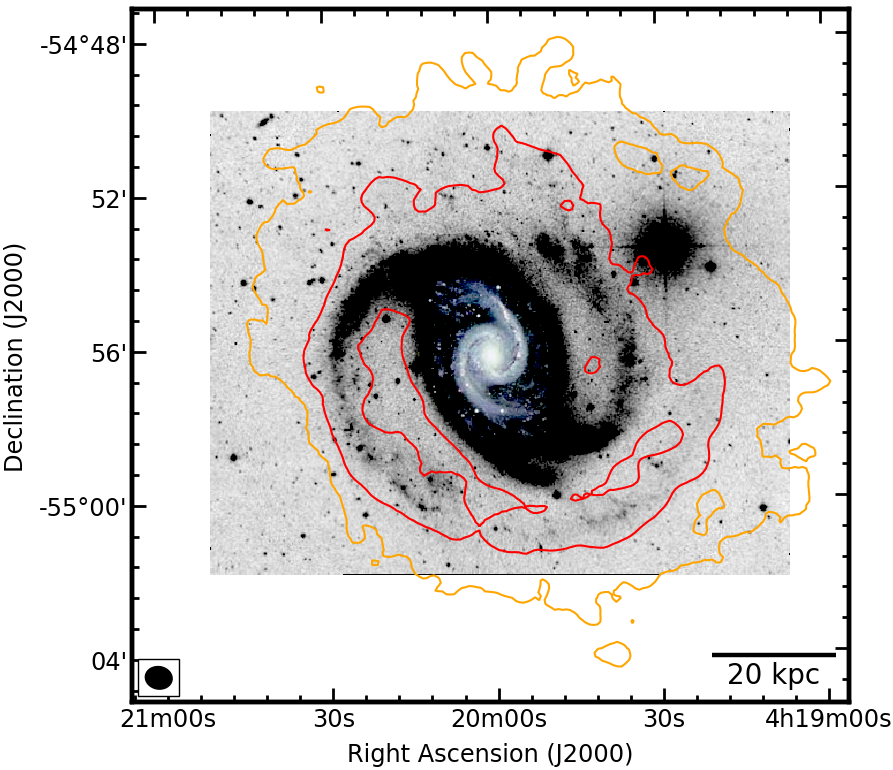
Figure 15: Deep optical image of NGC 1566 observed by David Malin and available at the Australian Astronomical Observatory database. The red and orange contours are at Hi column density values of $N_{\text{H{\sc{i}}}}\,=\,3.7\times 10^{20}\,$cm^-2 and $\,0.6\times 10^{20}\,$cm^-2, respectively. The black ellipse shows the restored beam of the ASKAP observations.

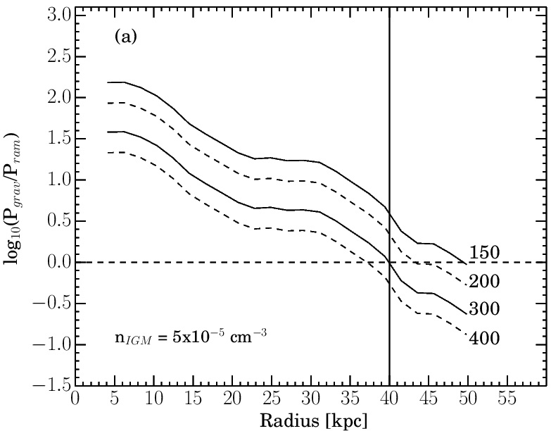
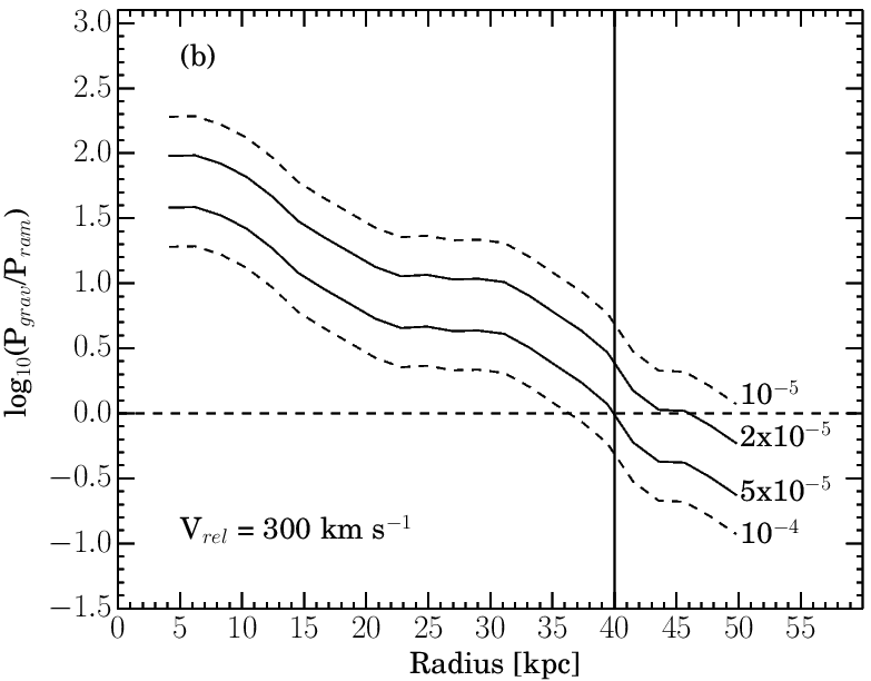
Figure 16: A comparison between the gravitational pressure and ram pressure ratio in the disc of NGC 1566 for different radii. (a) the pressure ratio assuming an IGM density value of n${}_{\text{IGM}}\,=\,5\times 10^{-5}\,$cm^-3 and relative velocities for NGC 1566 through the IGM of v${}_{\text{rel}}\,=\,150,\,200,\,300$ and $400\,$km s^-1. (b) the pressure ratio for constant velocity (v${}_{\text{rel}}\,=\,300\,$km s^-1) and four different IGM density values (n${}_{\text{IGM}}\,=\,1.0\times 10^{-5},\,2\times 10^{-5},\,5\times 10^{-5}\,$ and $1.0\times 10^{-4}$cm^-3). The horizontal dashed line represents the equality, above which the gaseous disc is dominated by gravity and below where ram pressure dominates and the disc is subjected to ram pressure stripping. The vertical line shows the radius at which the Hi column density of NGC 1566 is lopsided; At r$\,=\,40\,$kpc the column density of the south-eastern part of the Hi disc is nearly zero, while the north-western edge is more extended and smoothly declines with radius up to $\sim 50\,$kpc.

To examine the link between the observed asymmetries in the gas disc of NGC 1566 and ram pressure stripping, we follow the approach proposed by Gunn & Gott (1972) and compare the restoring force by the gravitational potential at the outer disc and the pressure from the IGM. The gas in the outer parts will remain intact to the halo as long as the ram pressure force is lower in magnitude than the pressure from the gravitational potential of the halo. For a disc galaxy with a gravitational potential $\phi(r)$ at a distance $r$ from the centre, the restoring force due to this gravitational potential will exert a pressure given by the following equation (Köppen et al., 2018; Roediger & Brüggen, 2006; Roediger & Hensler, 2005):

$$P_{\text{grav}}=\Sigma_{\text{gas}}({r})\Big{|}\frac{\partial\Phi(r)}{\partial z}\Big{|}_{\text{max}},$$ (12)

where the derivative denotes the maximum value of the restoring force at height $z$ above the disc. The height that corresponds to the maximum force is estimated by equating the second derivative of the gravitational potential $\frac{\partial^{2}\Phi(r)}{\partial z^{2}}$, to zero. On the other hand, the IGM will apply a pressure on the outer-most part of the disc that is given by the formula:

$$P_{\text{ram}}=\rho_{\text{IGM}}v_{\text{rel}}^{2},$$ (13)

where $\rho_{\text{IGM}}$ is the density of the IGM and $v_{\text{rel}}$ is the relative velocity of the galaxy. The ram pressure is capable of removing gas from the galaxy as it passes through the IGM only when $P_{\text{ram}}$ > $P_{\text{grav}}$. For our calculation, we make two assumptions. First, we only calculate the gravitational force due to the dark matter and neglect the restoring force from the stars and gas, i.e., we assume that the contribution from the baryonic matter is negligible. This is only true at the outer radii (refer to Figure 13) where the contribution of the dark matter dominates the total halo mass of NGC 1566 (Westmeier et al., 2011). The second necessary assumption is that NGC 1566 moves with an intermediate or “face-on” vector into the IGM, when ram pressure stripping is efficient (Quilis et al., 2000; Vollmer et al., 2001; Roediger & Hensler, 2005) but not directly in the line-of-sight, where morphological effects would be harder to discern . Based on the HI morphology and kinematics of this galaxy an encounter with the IGM at an intermediate inclination is favoured. To estimate the restoring force acting on the disc of NGC 1566, we use the NFW dark matter halo gravitational potential which is described by the equation:

$$\phi_{\text{NFW}}(r)=-\frac{GM_{\text{200}}\text{ln}\Big{(}1+\frac{r}{r_{s}}\Big{)}}{r\Big{[}\text{ln}(1+c)-\frac{c}{1+c}\Big{]}}.\\$$ (14)

Figure 16 presents the results of our simple analytic model, in which the ratio between $P_{\text{grav}}$ and $P_{\text{ram}}$ is calculated at different radii. In Figure 16a, we calculate this ratio assuming that the IGM density is constant (n${}_{\text{IGM}}\,=\,5\times 10^{-5}\,$cm^-3) and use different relative velocities for NGC 1566. This IGM density is similar to the Local Group gas density value (Rasmussen & Pedersen, 2001; Williams et al., 2005). Hence, we note that this adopted IGM density is a lower limit to the IGM density of NGC 1566 galaxy group. The NGC 1566 group has a halo mass (M${}_{\text{halo}}\sim 10^{13.5}\,$M_⊙; Kilborn et al., 2005) larger than the Local Group and consequently hotter/denser IGM gas is expected (Eke et al., 1998; Pratt et al., 2009; Barnes et al., 2017). In Figure 16b, we derive the same ratio adopting a constant relative velocity for NGC 1566 (v${}_{\text{rel}}\,=\,300\,$km s^-1) and different values for the IGM gas density. We use N-body simulations to predict the probability distribution of the relative velocity of NGC 1566 in the IGM following the orbital libraries described in Oman et al. (2013); Oman & Hudson (2016) and based on the projected coordinates of NGC 1566 (angular and velocity offsets) from the group centre (refer to Kilborn et al., 2005, for more information on this group). The relative velocity of a subhalo (galaxy) with a similar mass to NGC 1566 falling into a host halo (galaxy group), with a similar mass to NGC 1566 group, based on this analysis lies in the range between $250-500\,$km s^-1 at $99\,$per cent confidence. Figure 16 shows that the outer part of the Hi disc of NGC 1566 ($r\gtrsim 40\,$kpc), for certain values for v${}_{\text{rel}}\,$ and n${}_{\text{IGM}}$, can be affected by ram pressure winds in particular for n${}_{\text{IGM}}\gtrsim 5\times 10^{-5}\,$cm^-3 and v${}_{\text{rel}}\gtrsim 200\,$km s^-1. The highest IGM density adopted for NGC 1566 group and used in Figure 16b (n${}_{\text{IGM}}\gtrsim 10^{-4}\,$cm^-3) is consistent and in lower bound of the IGM density values reported for loose galaxy groups and derived from x-ray luminosities in Sengupta & Balasubramanyam (2006); Freeland et al. (2010). As expected for the inner regions the pressure due to the gravitational potential is much higher than the ram pressure force. We note that the ratio in the inner radii is higher than shown in the figure since, as already noted, we neglect the contributions from the stellar and the gaseous gravitational potentials (refer to Figures 12-13).

Even though our simple analytic approach suggests that ram pressure interaction with the IGM is the likely reason for the lopsidedness of the gas morphology of NGC 1566, the result is tentative. This is for two reasons. First, our ASKAP early science observation is not sensitive enough to probe Hi column densities below $10^{18}\,$cm^-2, which means that we can not rule out gas accretion as a plausible reason for the asymmetries seen in NGC 1566. The second caveat is that all the environmental processes that affect the Hi gas in galaxy groups such as tidal stripping by the host-halo (group), galaxy-galaxy encounters and ram pressure interaction operate at similar radial distances from the group centre. This is to say, as a galaxy approaches the centre of the host-halo and is within a distance of d/R${}_{\text{vir}}$ < $0.5$, where d is the physical distance from the group centre and R${}_{\text{vir}}$ is the virial radius of the group, it can experience ram pressure stripping from the IGM and/or can also tidally interact with nearby satellites (Marasco et al., 2016; Bahé et al., 2013). This adds to the complexity of disentangling the contributions of different external processes on the Hi gas content and morphology in galaxy groups. However, we think that sensitive Hi observations of large samples of galaxies, similar to those that WALLABY, APERTIF and MeerKAT will deliver in the next few years, will provide the Hi community with the opportunity to systematically study the Hi gas in group environments and help disentangling the contributions of these environmental processes.

5.2 Gas Content and Star Formation Rate in NGC 1566

To demonstrate the high atomic gas content of NGC 1566, we compare the Hi-to-stellar mass fraction of this galaxy to a sample of $25,000$ galaxies within $10^{9}\,$M${}_{\odot}\lesssim$ M${}_{*}\lesssim 10^{11.5}\,$M_⊙ and $0.02\leq z\leq 0.05$ obtained from the Sloan Digital Sky Survey. Brown et al. (2015) reported the Hi-to-stellar mass fractions of these galaxies using Hi data from the Arecibo Legacy Fast (ALFA) survey (Giovanelli et al., 2005). The stellar mass of NGC 1566 is $M_{*}\,=\,6.5\times 10^{10}\,$M_⊙, and has Hi-to-stellar mass fraction of log(M${}_{\text{H{\sc{i}}}}$/M_∗)$\,=\,-0.53\pm 0.10$. Figure 17a presents the Hi-to-stellar mass fraction vs. the stellar mass for Brown+15’s sample and for NGC 1566 (blue circle). It is evident that NGC 1566 has a relatively high Hi-to-stellar mass fraction in comparison with its counterparts that have a stellar mass of M_∗ $\sim 10^{10.81}\,$M_⊙. The average logarithmic Hi-to-stellar mass fraction of galaxies with M_∗ $\sim 10^{10.81}\,$M_⊙ is $\,-0.97$. We note that the uncertainty in the Hi-to-stellar mass of NGC 1566 is within the upper bounds of the scatter relation. This galaxy continues to have a relatively higher Hi-to-stellar mass fraction than the average at fixed stellar mass even when a smaller distance ($16.9\,$Mpc; the TF distance) is adopted (red circle in Figure 17a). Even though, the outskirts of NGC 1566 maybe subjected to ram-pressure interaction with the IGM, this scenario is not inconsistent with a high atomic gas fraction. Ram pressure stripping in group environments is likely to be subtle in comparison with galaxy clusters (Westmeier et al., 2011), in which the density of the intra-cluster medium is orders of magnitude higher than in the IGM (Eke et al., 1998; Pratt et al., 2009; Barnes et al., 2017).

Figure 17b shows the relation between the star formation rate and stellar mass for $\sim 10^{5}$ galaxies in the nearby Universe ($z<0.2$) observed in the Sloan Digital Sky Survey (SDSS) and reported in Brinchmann et al. (2004). The dashed-line shows the location of the main sequence of star formation for over $10^{5}$ galaxies in the local Universe (median redshift $z\,=\,0.2$) obtained by the Galaxy And Mass Assembly (GAMA) survey and reported in Davies et al. (2016). The blue circle shows the star formation rate of NGC 1566, log(SFR${}_{\text{H}\alpha}$[M_⊙ yr^-1])$\,=\,1.33\pm 0.1$. This figure highlights the high SFR in NGC 1566. The star formation in this galaxy (Figure 18) is mainly concentrated in the nucleus and the inner spiral arms and declines gradually following the outer spiral arms, in a similar fashion to the Hi gas. Further, this galaxy has a specific star formation rate (sSFR $=$ log (SFR/M_∗[yr^-1])) of $-9.48\pm 0.05$, which again places NGC 1566 above the average with respect to galaxies that have the same stellar mass, but within the scatter (Pan et al., 2018; Abramson et al., 2014). We note that the location of NGC 1566 in the mass-SFR parameter-space is subject to the distance adopted for this galaxy. For instance, if we use the TF distance ($16.9\,$Mpc) instead of the adopted distance in this work ($21.3\,$Mpc), the SFR and the stellar mass of NGC 1566 will be a factor of $0.63$ smaller. Thus, the SFR of NGC 1566 will become relatively closer to the median value per fixed stellar mass (red circle in Figure 17b), and NGC 1566 will appear less extreme in this parameter-space.

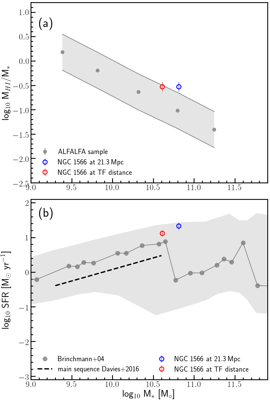
Figure 17: (a)The Hi-to-stellar mass fraction vs. the stellar mass for Brown+15’s galaxy sample (grey) and for NGC 1566 (blue circle). The red circle shows the location of NGC 1566 in the Hi-to-stellar mass fraction vs. M_∗ plane measured at a distance of $16.9\,$Mpc (the TF distance). The grey shaded regions delimit the y-axis scatter in the Brown+15’s galaxy sample. (b) The star formation rate vs. stellar mass for SDSS galaxies with $z<0.2$; the grey circles show the median value per stellar mass bin and the grey shaded region shows the scatter from the mean values along the SFR axis at a given stellar mass (Brinchmann et al., 2004). The dashed-line shows the location of the main sequence of star formation for the GAMA galaxy sample (Davies et al., 2016). The blue circle shows the location of NGC 1566 in the SFR-M_∗ plane. The red circle shows location of NGC 1566 in the SFR-M_∗ plane measured at the TF distance.

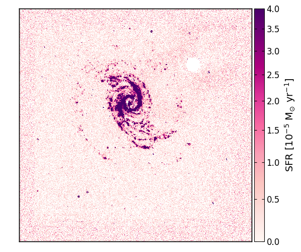
Figure 18: The SFR map based on the H$\alpha$ luminosity of NGC 1566 calculated following the SFR calibration of Meurer et al. (2009). The star formation is mainly concentrated in the inner spiral arms with some large Hii regions distributed in the outer arms.

6 Conclusion

In this work, we present our ASKAP Hi observations of NGC 1566, a grand design spiral in the Dorado group. Our major results and conclusions from this analysis are as follows:

• We measure an Hi mass of $1.94\times 10^{10}\,$M_⊙, assuming a distance of $21.3\,$Mpc, mainly concentrated in the spiral arms of NGC 1566. The Hi gas is distributed in an almost regular circular disc that extends well beyond the observed optical disc especially around the northern and western parts of NGC 1566. The Hi gas distribution also highlights the difference between the two outer arms better than in the optical. The eastern outer arm forms a regular arc shape that is more extended than the western arm, which is less regular or disturbed between PA$\,=\,270^{\circ}$ to $330^{\circ}$. The Hi disc of NGC 1566 is asymmetric: the south-eastern part of the Hi disc sharply declines beyond $\sim 30\,$kpc from the centre, whereas the north-western edge is more extended and smoothly declines with radius, up to a radius of $\sim 50\,$kpc.
  

• We measure the rotation curve of NGC 1566 out to a radius of $50$ kpc and estimate the dark matter content in this galaxy based on the ISO, NFW and Burkert dark matter halo profiles. We report dark matter fractions of $0.66$, $0.58$ and $0.62$ based on the ISO, NFW and Burkert profiles, respectively. Using our current ASKAP observations, we can not differentiate between these dark matter density profiles as the central region ($\sim 2\,$kpc) of NGC 1566 is not resolved. Higher angular resolution observations (few hundred parsec scales) are required for such analysis and for any conclusive findings (see for example Oh et al., 2015; de Blok et al., 2008; de Blok & Bosma, 2002). Such high angular resolution observations will be achieved in the next coming years using the $36$ ASKAP antennas (longest baseline of $6\,$km) and MeerKAT telescope (de Blok et al., 2016) for nearby galaxies. This will increase the number statistics of highly resolved rotation curves, and consequently better constraints on both the dark and baryonic matter distributions within these galaxies.
  

• We study the asymmetric Hi morphology of NGC 1566 and attempt to discriminate between three major environmental mechanisms that can cause asymmetries in galaxies, namely, ram pressure interactions with the IGM, galactic interactions as well as gas accretion from hosting/neighbouring filaments. We detect no nearby companion galaxy that may induce tidal forces on the Hi disc of NGC 1566 or tidal tails/plumes that are suggestive of such an encounter within the last $3.1\,$Gyr. The Hi mass detection limit of the ASKAP observations based on the $3\sigma$ noise level and over $40\,$km s^-1 channel widths is $\sim 2.2\times 10^{7}\,$M_⊙ beam^-1 at the assumed distance of NGC 1566 ($21.3\,$Mpc). We show, based on a simple analytic model, that ram pressure stripping can affect the Hi disc of NGC 1566 and is able to remove gas beyond a radius of $40$ kpc, using lower-limit values for the gas density of the IGM and the relative velocity of this galaxy. Further, we do not detect any clouds or filaments connected to, or in the nearby vicinity of, the Hi disc of NGC 1566. However, we are unable to completely rule out gas accretion from the local environment at lower column densities. Future Hi surveys with the SKA precursors and with large single dish telescopes, such as the Five-hundred-meter Aperture Spherical radio Telescope (FAST; Nan et al., 2011; Li & Pan, 2016; Zhang et al., 2019), will help probe the environment around galaxies and quantify the prevalence of gas accretion, interactions and ram pressure stripping in large sample of galaxies and their effects on the atomic gas morphology and kinematics.
  

• NGC 1566 has a relatively high Hi-to-stellar mass fraction in comparison with its counterparts that have the same stellar mass. The average logarithmic Hi-to-stellar mass fraction of galaxies with M_∗ $\sim 10^{10.81}\,$M_⊙ is log(M${}_{\text{H{\sc{i}}}}$/M_∗)$=\,-0.97$. while for NGC 1566 is log(M${}_{\text{H{\sc{i}}}}$/M_∗)$\,=\,-0.53\pm 0.1$. Further, NGC 1566 possesses a specific star formation rate (sSFR $=$ log SFR/M_∗[yr^-1]) of $-9.48\pm 0.05$, which is again above the average with respect to galaxies that have the same stellar mass, but within the scatter (Pan et al., 2018; Abramson et al., 2014). However, the location of NGC 1566 in the mass-SFR parameter-space is dependent on the assumed distance, for which there remains significant uncertainty.
  

Appendix A The Atomic Gas Morphology in NGC 1566

Figure 19 shows a 3D position-position-velocity interactive view of the Hi cube of NGC 1566 made using the Astronomy Hi Extension for 3D Slicer (SlicerAstro; Punzo et al., 2017, 2016) . The reader can actively interact (rotate, drag, zoom-in or out) with the 3D plot using Adobe Reader 9.

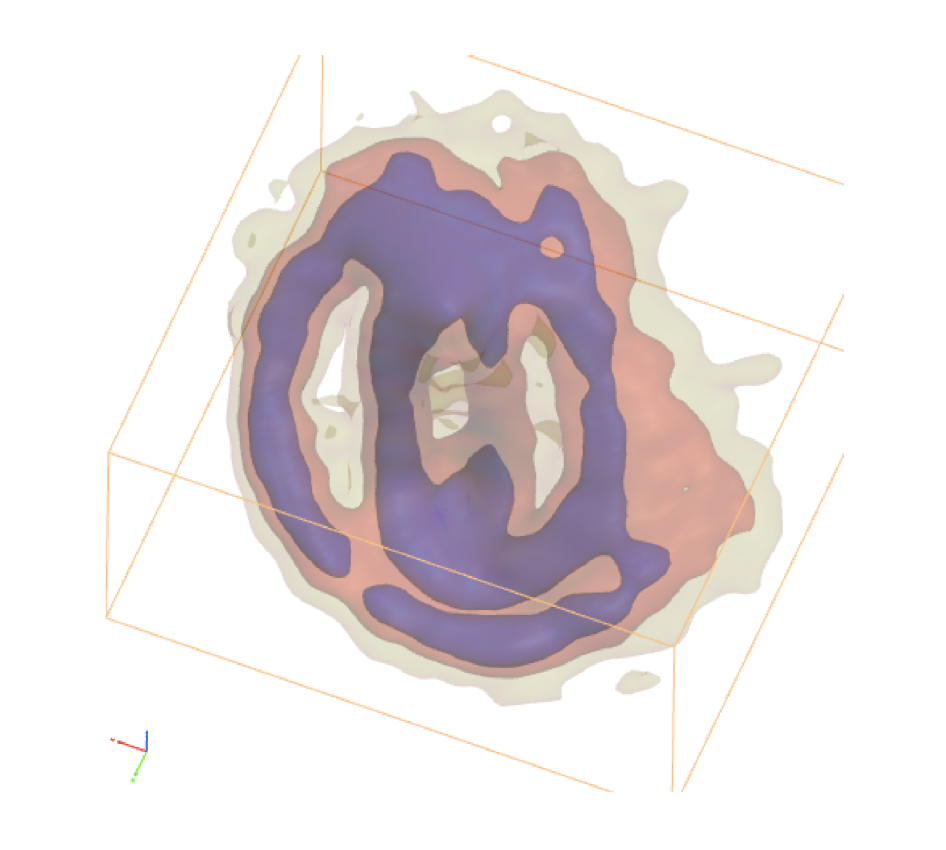
Figure 19: 3D rendering of the Hi cube of NGC 1566 based on our ASKAP early science observations, the three axes in this visualisation are RA, Dec, and the velocity . To improve the visualisation, pixels with flux values $>0.088,0.037\,$Jy beam^-1 km^-1 and $0.0017\,$Jy beam^-1 km^-1 are rendered with blue, red and green colors, respectively.

References

- Abadi et al. (1999) Abadi M. G., Moore B., Bower R. G., 1999, MNRAS, 308, 947
- Abramowicz et al. (1986) Abramowicz M. A., Lasota J. P., Xu C., 1986, in Swarup G., Kapahi V. K., eds, IAU Symposium Vol. 119, Quasars. pp 371–380
- Abramson et al. (2014) Abramson L. E., Kelson D. D., Dressler A., Poggianti B., Gladders M. D., Oemler Jr. A., Vulcani B., 2014, ApJ, 785, L36
- Acreman et al. (2003) Acreman D. M., Stevens I. R., Ponman T. J., Sakelliou I., 2003, MNRAS, 341, 1333
- Agüero et al. (2004) Agüero E. L., Díaz R. J., Bajaja E., 2004, A&A, 414, 453
- Allen et al. (1985) Allen R. J., Ekers R. D., Terlouw J. P., 1985, in di Gesu V., Scarsi L., Crane P., Friedman J. H., Levialdi S., eds, Data Analysis in Astronomy. p. 271
- Alloin et al. (1986) Alloin D., Pelat D., Phillips M. M., Fosbury R. A. E., Freeman K., 1986, ApJ, 308, 23
- Alonso-Herrero et al. (2000) Alonso-Herrero A., Rieke G. H., Rieke M. J., Scoville N. Z., 2000, ApJ, 532, 845
- Alonso et al. (2004) Alonso M. S., Tissera P. B., Coldwell G., Lambas D. G., 2004, MNRAS, 352, 1081
- Antonuccio-Delogu et al. (2002) Antonuccio-Delogu V., Becciani U., van Kampen E., Pagliaro A., Romeo A. B., Colafrancesco S., Germaná A., Gambera M., 2002, MNRAS, 332, 7
- Avila-Reese et al. (2005) Avila-Reese V., Colín P., Gottlöber S., Firmani C., Maulbetsch C., 2005, ApJ, 634, 51
- Bahé et al. (2013) Bahé Y. M., McCarthy I. G., Balogh M. L., Font A. S., 2013, MNRAS, 430, 3017
- Bahé et al. (2019) Bahé Y. M., et al., 2019, MNRAS, 485, 2287
- Bajaja et al. (1995) Bajaja E., Wielebinski R., Reuter H.-P., Harnett J. I., Hummel E., 1995, A&AS, 114, 147
- Baldwin et al. (1980) Baldwin J. E., Lynden-Bell D., Sancisi R., 1980, MNRAS, 193, 313
- Balogh et al. (1997) Balogh M. L., Morris S. L., Yee H. K. C., Carlberg R. G., Ellingson E., 1997, ApJ, 488, L75
- Balogh et al. (2004) Balogh M., et al., 2004, MNRAS, 348, 1355
- Balsara et al. (1994) Balsara D., Livio M., O’Dea C. P., 1994, ApJ, 437, 83
- Barnes & Hernquist (1991) Barnes J. E., Hernquist L. E., 1991, ApJ, 370, L65
- Barnes et al. (2017) Barnes D. J., et al., 2017, MNRAS, 471, 1088
- Begeman (1989) Begeman K. G., 1989, A&A, 223, 47
- Begeman et al. (1991) Begeman K. G., Broeils A. H., Sanders R. H., 1991, MNRAS, 249, 523
- Blanton & Moustakas (2009) Blanton M. R., Moustakas J., 2009, ARA&A, 47, 159
- Blanton et al. (2005) Blanton M. R., Eisenstein D., Hogg D. W., Schlegel D. J., Brinkmann J., 2005, ApJ, 629, 143
- Bolatto et al. (2002) Bolatto A. D., Simon J. D., Leroy A., Blitz L., 2002, ApJ, 565, 238
- Boselli & Gavazzi (2006) Boselli A., Gavazzi G., 2006, PASP, 118, 517
- Bournaud et al. (2005) Bournaud F., Combes F., Jog C. J., Puerari I., 2005, A&A, 438, 507
- Brandl et al. (2009) Brandl B. R., et al., 2009, ApJ, 699, 1982
- Braun & Thilker (2004) Braun R., Thilker D. A., 2004, A&A, 417, 421
- Brinchmann et al. (2004) Brinchmann J., Charlot S., White S. D. M., Tremonti C., Kauffmann G., Heckman T., Brinkmann J., 2004, MNRAS, 351, 1151
- Brown et al. (2015) Brown T., Catinella B., Cortese L., Kilborn V., Haynes M. P., Giovanelli R., 2015, MNRAS, 452, 2479
- Brown et al. (2017) Brown T., et al., 2017, MNRAS, 466, 1275
- Burkert (1995) Burkert A., 1995, ApJ, 447, L25
- Casertano (1983) Casertano S., 1983, MNRAS, 203, 735
- Cayatte et al. (1990) Cayatte V., van Gorkom J. H., Balkowski C., Kotanyi C., 1990, AJ, 100, 604
- Chen et al. (2017) Chen Y.-C., et al., 2017, MNRAS, 466, 1880
- Chung et al. (2006) Chung A., Koribalski B., Bureau M., van Gorkom J. H., 2006, MNRAS, 370, 1565
- Chung et al. (2007) Chung A., van Gorkom J. H., Kenney J. D. P., Vollmer B., 2007, ApJ, 659, L115
- Chung et al. (2009) Chung A., van Gorkom J. H., Kenney J. D. P., Crowl H., Vollmer B., 2009, AJ, 138, 1741
- Cibinel et al. (2013) Cibinel A., et al., 2013, ApJ, 777, 116
- Combes et al. (2014) Combes F., et al., 2014, A&A, 565, A97
- Comte & Duquennoy (1982) Comte G., Duquennoy A., 1982, A&A, 114, 7
- Cornwell et al. (1992) Cornwell T. J., Uson J. M., Haddad N., 1992, A&A, 258, 583
- Cortese et al. (2011) Cortese L., Catinella B., Boissier S., Boselli A., Heinis S., 2011, MNRAS, 415, 1797
- Croton et al. (2005) Croton D. J., et al., 2005, MNRAS, 356, 1155
- Davies & Lewis (1973) Davies R. D., Lewis B. M., 1973, MNRAS, 165, 231
- Davies et al. (2016) Davies L. J. M., et al., 2016, MNRAS, 461, 458
- DeBoer et al. (2009) DeBoer D. R., et al., 2009, IEEE Proceedings, 97, 1507
- Dénes et al. (2016) Dénes H., Kilborn V. A., Koribalski B. S., Wong O. I., 2016, MNRAS, 455, 1294
- Dewdney et al. (2009) Dewdney P. E., Hall P. J., Schilizzi R. T., Lazio T. J. L. W., 2009, IEEE Proceedings, 97, 1482
- Dickey & Gavazzi (1991) Dickey J. M., Gavazzi G., 1991, ApJ, 373, 347
- Dressler (1980) Dressler A., 1980, ApJ, 236, 351
- Dressler et al. (1997) Dressler A., et al., 1997, ApJ, 490, 577
- Dubinski et al. (1996) Dubinski J., Mihos J. C., Hernquist L., 1996, ApJ, 462, 576
- Duffy et al. (2012) Duffy A. R., Meyer M. J., Staveley-Smith L., Bernyk M., Croton D. J., Koribalski B. S., Gerstmann D., Westerlund S., 2012, MNRAS, 426, 3385
- Ehle et al. (1996) Ehle M., Beck R., Haynes R. F., Vogler A., Pietsch W., Elmouttie M., Ryder S., 1996, A&A, 306, 73
- Eke et al. (1998) Eke V. R., Navarro J. F., Frenk C. S., 1998, ApJ, 503, 569
- Elagali et al. (2018a) Elagali A., Wong O. I., Oh S.-H., Staveley-Smith L., Koribalski B. S., Bekki K., Zwaan M., 2018a, MNRAS, 476, 5681
- Elagali et al. (2018b) Elagali A., Lagos C. D. P., Wong O. I., Staveley-Smith L., Trayford J. W., Schaller M., Yuan T., Abadi M. G., 2018b, MNRAS, 481, 2951
- Fakhouri & Ma (2009) Fakhouri O., Ma C.-P., 2009, MNRAS, 394, 1825
- Farouki & Shapiro (1982) Farouki R. T., Shapiro S. L., 1982, ApJ, 259, 103
- Fazio et al. (2004) Fazio G. G., et al., 2004, ApJS, 154, 10
- Fogarty et al. (2014) Fogarty L. M. R., et al., 2014, MNRAS, 443, 485
- Freeland et al. (2010) Freeland E., Sengupta C., Croston J. H., 2010, MNRAS, 409, 1518
- Gavazzi & Jaffe (1986) Gavazzi G., Jaffe W., 1986, ApJ, 310, 53
- Giovanelli et al. (2005) Giovanelli R., et al., 2005, AJ, 130, 2598
- Glass (2004) Glass I. S., 2004, MNRAS, 350, 1049
- Gómez et al. (2003) Gómez P. L., et al., 2003, ApJ, 584, 210
- Gooch (1996) Gooch R., 1996, in Jacoby G. H., Barnes J., eds, Astronomical Society of the Pacific Conference Series Vol. 101, Astronomical Data Analysis Software and Systems V. p. 80
- Gunn & Gott (1972) Gunn J. E., Gott III J. R., 1972, ApJ, 176, 1
- Hackwell & Schweizer (1983) Hackwell J. A., Schweizer F., 1983, ApJ, 265, 643
- Hahn et al. (2007) Hahn O., Porciani C., Carollo C. M., Dekel A., 2007, MNRAS, 375, 489
- Hay & O’Sullivan (2008) Hay S. G., O’Sullivan J. D., 2008, Radio Science, 43, RS6S04
- Haynes & Giovanelli (1986) Haynes M. P., Giovanelli R., 1986, ApJ, 306, 466
- Heald et al. (2016) Heald G., et al., 2016, MNRAS, 462, 1238
- Hernquist & Quinn (1988) Hernquist L., Quinn P. J., 1988, ApJ, 331, 682
- Hernquist & Quinn (1989) Hernquist L., Quinn P. J., 1989, ApJ, 342, 1
- Houghton (2015) Houghton R. C. W., 2015, MNRAS, 451, 3427
- Jaffé et al. (2018) Jaffé Y. L., et al., 2018, MNRAS, 476, 4753
- Johnston et al. (2007) Johnston S., et al., 2007, Publ. Astron. Soc. Australia, 24, 174
- Johnston et al. (2008) Johnston S., et al., 2008, Experimental Astronomy, 22, 151
- Jonas & MeerKAT Team (2016) Jonas J., MeerKAT Team 2016, in Proceedings of MeerKAT Science: On the Pathway to the SKA. 25-27 May, 2016 Stellenbosch, South Africa. p. 1
- Jung et al. (2018) Jung S. L., Choi H., Wong O. I., Kimm T., Chung A., Yi S. K., 2018, preprint, (arXiv:1809.01684)
- Kado-Fong et al. (2018) Kado-Fong E., et al., 2018, preprint, (arXiv:1805.05970)
- Kamphuis et al. (2015) Kamphuis P., Józsa G. I. G., Oh S.-. H., Spekkens K., Urbancic N., Serra P., Koribalski B. S., Dettmar R.-J., 2015, MNRAS, 452, 3139
- Kantharia et al. (2005) Kantharia N. G., Ananthakrishnan S., Nityananda R., Hota A., 2005, A&A, 435, 483
- Kauffmann et al. (2004) Kauffmann G., White S. D. M., Heckman T. M., Ménard B., Brinchmann J., Charlot S., Tremonti C., Brinkmann J., 2004, MNRAS, 353, 713
- Kent (1986) Kent S. M., 1986, AJ, 91, 1301
- Kent (1987) Kent S. M., 1987, AJ, 93, 816
- Kilborn et al. (2005) Kilborn V. A., Koribalski B. S., Forbes D. A., Barnes D. G., Musgrave R. C., 2005, MNRAS, 356, 77
- Kilborn et al. (2009) Kilborn V. A., Forbes D. A., Barnes D. G., Koribalski B. S., Brough S., Kern K., 2009, MNRAS, 400, 1962
- Köppen et al. (2018) Köppen J., Jáchym P., Taylor R., Palouš J., 2018, MNRAS, 479, 4367
- Koribalski (2012) Koribalski B. S., 2012, Publ. Astron. Soc. Australia, 29, 359
- Kormendy (1984) Kormendy J., 1984, ApJ, 286, 116
- Kourkchi & Tully (2017) Kourkchi E., Tully R. B., 2017, ApJ, 843, 16
- Kozłowski et al. (2016) Kozłowski S., Kochanek C. S., Ashby M. L. N., Assef R. J., Brodwin M., Eisenhardt P. R., Jannuzi B. T., Stern D., 2016, ApJ, 817, 119
- Kreckel et al. (2012) Kreckel K., Platen E., Aragón-Calvo M. A., van Gorkom J. H., van de Weygaert R., van der Hulst J. M., Beygu B., 2012, AJ, 144, 16
- Kregel et al. (2002) Kregel M., van der Kruit P. C., de Grijs R., 2002, MNRAS, 334, 646
- Lagos et al. (2018) Lagos C. d. P., et al., 2018, MNRAS, 473, 4956
- Laine et al. (2014) Laine S., et al., 2014, MNRAS, 444, 3015
- Larson (1972) Larson R. B., 1972, Nature, 236, 21
- Larson et al. (1980) Larson R. B., Tinsley B. M., Caldwell C. N., 1980, ApJ, 237, 692
- Lee-Waddell et al. (2019) Lee-Waddell K., et al., 2019, arXiv e-prints, p. arXiv:1901.00241
- Levenson et al. (2009) Levenson N. A., Radomski J. T., Packham C., Mason R. E., Schaefer J. J., Telesco C. M., 2009, ApJ, 703, 390
- Lewis et al. (2002) Lewis I., et al., 2002, MNRAS, 334, 673
- Li & Pan (2016) Li D., Pan Z., 2016, Radio Science, 51, 1060
- Loveday et al. (1992) Loveday J., Peterson B. A., Efstathiou G., Maddox S. J., 1992, ApJ, 390, 338
- Magri et al. (1988) Magri C., Haynes M. P., Forman W., Jones C., Giovanelli R., 1988, ApJ, 333, 136
- Mapelli et al. (2008) Mapelli M., Moore B., Bland-Hawthorn J., 2008, MNRAS, 388, 697
- Marasco et al. (2016) Marasco A., Crain R. A., Schaye J., Bahé Y. M., van der Hulst T., Theuns T., Bower R. G., 2016, MNRAS, 461, 2630
- Martínez-Delgado et al. (2010) Martínez-Delgado D., et al., 2010, AJ, 140, 962
- Martínez-Delgado et al. (2015) Martínez-Delgado D., D’Onghia E., Chonis T. S., Beaton R. L., Teuwen K., GaBany R. J., Grebel E. K., Morales G., 2015, AJ, 150, 116
- Masters et al. (2006) Masters K. L., Springob C. M., Haynes M. P., Giovanelli R., 2006, ApJ, 653, 861
- McConnachie et al. (2007) McConnachie A. W., Venn K. A., Irwin M. J., Young L. M., Geehan J. J., 2007, ApJ, 671, L33
- McNaught-Roberts et al. (2014) McNaught-Roberts T., et al., 2014, MNRAS, 445, 2125
- Merluzzi et al. (2016) Merluzzi P., Busarello G., Dopita M. A., Haines C. P., Steinhauser D., Bourdin H., Mazzotta P., 2016, MNRAS, 460, 3345
- Meurer et al. (2006) Meurer G. R., et al., 2006, ApJS, 165, 307
- Meurer et al. (2009) Meurer G. R., et al., 2009, The Astrophysical Journal, 695, 765
- Michel-Dansac et al. (2010) Michel-Dansac L., et al., 2010, ApJ, 717, L143
- Moreno et al. (2015) Moreno J., Torrey P., Ellison S. L., Patton D. R., Bluck A. F. L., Bansal G., Hernquist L., 2015, MNRAS, 448, 1107
- Nan et al. (2011) Nan R., et al., 2011, International Journal of Modern Physics D, 20, 989
- Navarro et al. (1996) Navarro J. F., Frenk C. S., White S. D. M., 1996, ApJ, 462, 563
- Navarro et al. (1997) Navarro J. F., Frenk C. S., White S. D. M., 1997, ApJ, 490, 493
- Norberg et al. (2001) Norberg P., et al., 2001, MNRAS, 328, 64
- Oemler (1974) Oemler Jr. A., 1974, ApJ, 194, 1
- Oh et al. (2008) Oh S.-H., de Blok W. J. G., Walter F., Brinks E., Kennicutt Jr. R. C., 2008, AJ, 136, 2761
- Oh et al. (2015) Oh S.-H., et al., 2015, AJ, 149, 180
- Okamoto & Habe (1999) Okamoto T., Habe A., 1999, ApJ, 516, 591
- Oman & Hudson (2016) Oman K. A., Hudson M. J., 2016, MNRAS, 463, 3083
- Oman et al. (2013) Oman K. A., Hudson M. J., Behroozi P. S., 2013, MNRAS, 431, 2307
- Omar & Dwarakanath (2005) Omar A., Dwarakanath K. S., 2005, Journal of Astrophysics and Astronomy, 26, 1
- Oosterloo et al. (2007) Oosterloo T., Fraternali F., Sancisi R., 2007, AJ, 134, 1019
- Osmond & Ponman (2004) Osmond J. P. F., Ponman T. J., 2004, MNRAS, 350, 1511
- Pan et al. (2018) Pan H.-A., et al., 2018, ApJ, 854, 159
- Paulino-Afonso et al. (2018) Paulino-Afonso A., Sobral D., Darvish B., Ribeiro B., Stroe A., Best P., Afonso J., Matsuda Y., 2018, A&A, 620, A186
- Pence et al. (1990) Pence W. D., Taylor K., Atherton P., 1990, ApJ, 357, 415
- Peng et al. (2010) Peng Y.-j., et al., 2010, ApJ, 721, 193
- Poggianti et al. (1999) Poggianti B. M., Smail I., Dressler A., Couch W. J., Barger A. J., Butcher H., Ellis R. S., Oemler Augustus J., 1999, ApJ, 518, 576
- Pop et al. (2018) Pop A.-R., Pillepich A., Amorisco N. C., Hernquist L., 2018, MNRAS, 480, 1715
- Porter et al. (2008) Porter S. C., Raychaudhury S., Pimbblet K. A., Drinkwater M. J., 2008, MNRAS, 388, 1152
- Postman et al. (2005) Postman M., et al., 2005, ApJ, 623, 721
- Pratt et al. (2009) Pratt G. W., Croston J. H., Arnaud M., Böhringer H., 2009, A&A, 498, 361
- Punzo et al. (2016) Punzo D., van der Hulst T., Roerdink J., Fillion-Robin J.-C., 2016, SlicerAstro: Astronomy (HI) extension for 3D Slicer, Astrophysics Source Code Library (ascl:1611.021)
- Punzo et al. (2017) Punzo D., van der Hulst J. M., Roerdink J. B. T. M., Fillion-Robin J. C., Yu L., 2017, Astronomy and Computing, 19, 45
- Putman et al. (2012) Putman M. E., Peek J. E. G., Joung M. R., 2012, ARA&A, 50, 491
- Quilis et al. (2000) Quilis V., Moore B., Bower R., 2000, Science, 288, 1617
- Rahmani et al. (2018) Rahmani H., et al., 2018, MNRAS, 474, 254
- Ramos-Martínez et al. (2018) Ramos-Martínez M., Gómez G. C., Pérez-Villegas Á., 2018, MNRAS, 476, 3781
- Randall et al. (2008) Randall S., Nulsen P., Forman W. R., Jones C., Machacek M., Murray S. S., Maughan B., 2008, ApJ, 688, 208
- Rasmussen & Pedersen (2001) Rasmussen J., Pedersen K., 2001, ApJ, 559, 892
- Rasmussen et al. (2012) Rasmussen J., et al., 2012, ApJ, 747, 31
- Reach et al. (2005) Reach W. T., et al., 2005, PASP, 117, 978
- Reeves et al. (2016) Reeves S. N., et al., 2016, MNRAS, 457, 2613
- Reichard et al. (2008) Reichard T. A., Heckman T. M., Rudnick G., Brinchmann J., Kauffmann G., 2008, ApJ, 677, 186
- Reunanen et al. (2002) Reunanen J., Kotilainen J. K., Prieto M. A., 2002, MNRAS, 331, 154
- Reynolds et al. (2019) Reynolds T. N., et al., 2019, MNRAS, 482, 3591
- Roediger & Brüggen (2006) Roediger E., Brüggen M., 2006, MNRAS, 369, 567
- Roediger & Hensler (2005) Roediger E., Hensler G., 2005, A&A, 433, 875
- Rokaki et al. (1993) Rokaki E., Collin-Souffrin S., Magnan C., 1993, A&A, 272, 8
- Ruan et al. (2014) Ruan J. J., Anderson S. F., Dexter J., Agol E., 2014, ApJ, 783, 105
- Ruggiero & Lima Neto (2017) Ruggiero R., Lima Neto G. B., 2017, MNRAS, 468, 4107
- Salucci & Burkert (2000) Salucci P., Burkert A., 2000, ApJ, 537, L9
- Sancisi et al. (2008) Sancisi R., Fraternali F., Oosterloo T., van der Hulst T., 2008, A&ARv, 15, 189
- Sanders et al. (2003) Sanders D. B., Mazzarella J. M., Kim D.-C., Surace J. A., Soifer B. T., 2003, AJ, 126, 1607
- Sault (1994) Sault R. J., 1994, A&AS, 107, 55
- Sault et al. (1995) Sault R. J., Teuben P. J., Wright M. C. H., 1995, in Shaw R. A., Payne H. E., Hayes J. J. E., eds, Astronomical Society of the Pacific Conference Series Vol. 77, Astronomical Data Analysis Software and Systems IV. p. 433 (arXiv:astro-ph/0612759)
- Schinckel & Bock (2016) Schinckel A. E. T., Bock D. C.-J., 2016, in Ground-based and Airborne Telescopes VI. p. 99062A, doi:10.1117/12.2233920
- Schröder et al. (2001) Schröder A., Drinkwater M. J., Richter O.-G., 2001, A&A, 376, 98
- Sengupta & Balasubramanyam (2006) Sengupta C., Balasubramanyam R., 2006, MNRAS, 369, 360
- Sengupta et al. (2007) Sengupta C., Balasubramanyam R., Dwarakanath K. S., 2007, MNRAS, 378, 137
- Serra et al. (2015) Serra P., et al., 2015, MNRAS, 448, 1922
- Sheen et al. (2017) Sheen Y.-K., et al., 2017, ApJ, 840, L7
- Solanes et al. (2001) Solanes J. M., Manrique A., García-Gómez C., González-Casado G., Giovanelli R., Haynes M. P., 2001, ApJ, 548, 97
- Staveley-Smith et al. (1996) Staveley-Smith L., et al., 1996, Publ. Astron. Soc. Australia, 13, 243
- Thomas et al. (2010) Thomas D., Maraston C., Schawinski K., Sarzi M., Silk J., 2010, MNRAS, 404, 1775
- Toomre & Toomre (1972) Toomre A., Toomre J., 1972, ApJ, 178, 623
- Tosi (1988) Tosi M., 1988, A&A, 197, 33
- Tully & Fisher (1977) Tully R. B., Fisher J. R., 1977, A&A, 54, 661
- Verheijen et al. (2008) Verheijen M. A. W., Oosterloo T. A., van Cappellen W. A., Bakker L., Ivashina M. V., van der Hulst J. M., 2008, in Minchin R., Momjian E., eds, American Institute of Physics Conference Series Vol. 1035, The Evolution of Galaxies Through the Neutral Hydrogen Window. pp 265–271 (arXiv:0806.0234), doi:10.1063/1.2973599
- Vollmer (2009) Vollmer B., 2009, A&A, 502, 427
- Vollmer et al. (2001) Vollmer B., Cayatte V., Balkowski C., Duschl W. J., 2001, ApJ, 561, 708
- Vulcani et al. (2018) Vulcani B., et al., 2018, MNRAS, 480, 3152
- Walsh (1997) Walsh W., 1997, PhD thesis, Univ. New South Wales , (1997)
- Werner et al. (2004) Werner M. W., et al., 2004, ApJS, 154, 1
- Westmeier et al. (2011) Westmeier T., Braun R., Koribalski B. S., 2011, MNRAS, 410, 2217
- White et al. (1991) White D. A., Fabian A. C., Forman W., Jones C., Stern C., 1991, ApJ, 375, 35
- Williams et al. (2005) Williams R. J., et al., 2005, ApJ, 631, 856
- Wong (2007) Wong O. I., 2007, PhD thesis, University of Melbourne
- Woo & Urry (2002) Woo J.-H., Urry C. M., 2002, ApJ, 579, 530
- Xie et al. (2018) Xie L., De Lucia G., Wilman D. J., Fossati M., Erwin P., Gutiérrez L., Kulkarni S. K., 2018, MNRAS, 480, 3812
- Yoon et al. (2017) Yoon H., Chung A., Smith R., Jaffé Y. L., 2017, ApJ, 838, 81
- Yozin & Bekki (2014) Yozin C., Bekki K., 2014, MNRAS, 439, 1948
- Yun et al. (1994) Yun M. S., Ho P. T. P., Lo K. Y., 1994, Nature, 372, 530
- Zhang et al. (2019) Zhang K., et al., 2019, arXiv e-prints, p. arXiv:1903.06402
- Zheng et al. (2017) Zheng Z., et al., 2017, MNRAS, 465, 4572
- Zuo et al. (2012) Zuo W., Wu X.-B., Liu Y.-Q., Jiao C.-L., 2012, ApJ, 758, 104
- da Silva et al. (2017) da Silva P., Steiner J. E., Menezes R. B., 2017, MNRAS, 470, 3850
- de Blok (2010) de Blok W. J. G., 2010, Advances in Astronomy, 2010, 789293
- de Blok & Bosma (2002) de Blok W. J. G., Bosma A., 2002, A&A, 385, 816
- de Blok et al. (2001) de Blok W. J. G., McGaugh S. S., Bosma A., Rubin V. C., 2001, ApJ, 552, L23
- de Blok et al. (2008) de Blok W. J. G., Walter F., Brinks E., Trachternach C., Oh S.-H., Kennicutt Jr. R. C., 2008, AJ, 136, 2648
- de Blok et al. (2014a) de Blok W. J. G., et al., 2014a, A&A, 566, A80
- de Blok et al. (2014b) de Blok W. J. G., et al., 2014b, A&A, 569, A68
- de Blok et al. (2016) de Blok W. J. G., et al., 2016, in Proceedings of MeerKAT Science: On the Pathway to the SKA. 25-27 May, 2016 Stellenbosch, South Africa (MeerKAT2016). p. 7 (arXiv:1709.08458)
- de Vaucouleurs (1973) de Vaucouleurs G., 1973, ApJ, 181, 31
- de Vaucouleurs et al. (1976) de Vaucouleurs G., de Vaucouleurs A., Corwin J. R., 1976, in Second reference catalogue of bright galaxies, Vol. 1976, p. Austin: University of Texas Press..
- van der Hulst et al. (1992) van der Hulst J. M., Terlouw J. P., Begeman K. G., Zwitser W., Roelfsema P. R., 1992, in Worrall D. M., Biemesderfer C., Barnes J., eds, Astronomical Society of the Pacific Conference Series Vol. 25, Astronomical Data Analysis Software and Systems I. p. 131
- van der Kruit & Searle (1981) van der Kruit P. C., Searle L., 1981, A&A, 95, 105