Phase Space Analysis for Anisotropic Universe with Nonlinear Bulk Viscosity

Abstract

In this paper, we discuss phase space analysis of locally rotationally symmetric Bianchi type I universe model by taking a noninteracting mixture of dust like and viscous radiation like fluid whose viscous pressure satisfies a nonlinear version of the Israel-Stewart transport equation. An autonomous system of equations is established by defining normalized dimensionless variables. In order to investigate stability of the system, we evaluate corresponding critical points for different values of the parameters. We also compute power-law scale factor whose behavior indicates different phases of the universe model. It is found that our analysis does not provide a complete immune from fine-tuning because the exponentially expanding solution occurs only for a particular range of parameters. We conclude that stable solutions exist in the presence of nonlinear model for bulk viscosity with different choices of the constant parameter $m$ for anisotropic universe.

Keywords: Phase space analysis; Bianchi type I universe; Bulk viscosity.
PACS: 04.20.Cv; 95.36.+x; 98.80.Jk.

1 Introduction

It is evident through many astronomical observations that our universe is undergoing an accelerated expansion at its present stage. This primal fact is supported by the observational probes of various astronomical advances (type Ia supernova, large scale structure and cosmic microwave background radiation (CMBR)) that puts forward an open question on the current understanding of fundamental physics [1]. These observations suggest two cosmic phases of accelerated expansion, i.e., the cosmic state before radiation (the primordial inflationary era) and ultimately the present cosmos phase after the matter dominated era. In the last couple of decades, it is speculated that some mysterious source of energy with unusual anti-gravitational force is responsible for the current cosmic expansion dubbed as dark energy (DE).

The existence of this energy with large negative pressure does not cluster at large scales. The study of the dominant constituents of matter distribution in the universe has remained one of the most debatable issues. Recent observations show that the visible part of our universe is made up of baryonic matter contributing only $5\%$ of the total budget while the remaining ingredients yield the total energy density composed of non-baryonic fluids ($68\%$ DE and $27\%$ dark matter) [2]. The dark matter is an unusual material which can be detected through its gravitational effects and neither emits nor absorbs light [3].

In order to study the ambiguous nature of DE, several proposals have been introduced in literature among them a small cosmological constant ($\Lambda$) governed by a negative equation of state (EoS) parameter ($\omega=-1$) is considered to be the simplest characterization of DE. However, this identification has two well-known problems, i.e., fine-tuning and cosmic coincidence. In addition, there are several dynamical models which can be considered as an alternative to $\Lambda$. These candidates involve scalar field models like quintessence [4], phantom model [5], tachyon field [6] and k-essence [7] that also suggest expanding behavior of the universe. Another approach involves the generalization of simple barotropic EoS to more exotic forms such as Chaplygin gas [8] and its modification [9].

It has been suggested that a fluid with bulk viscosity may cause an accelerated expansion of the universe models without cosmological constant or scalar field [10]. The bulk viscosity refers to the measure of pressure required to restore an equilibrium state when cosmic expansion of any fluid occurs in an expanding universe scenario. In case of thermodynamics, bulk viscosity occurs due to its deviation from local thermodynamical equilibrium in any physical system [11]. Our main concern is to explore another approach which tends to minimize the exotic forms of matter by introducing dissipation through viscous effects of fluids. Bulk viscous pressure provides the dissipative contribution which has a significant relevance in homogeneous universe scenarios.

A phase space is a space describing all possible states (position and momentum) corresponding to each point of the system. The study of possible stable late-time attractors has attained remarkable significance for different universe models. A phase space analysis manifests dynamical behavior of a cosmological model through a global view by reducing complexity of the equations (converting the system of equations to an autonomous system). This analysis is helpful to comprehend different patterns of evolution. A linearly stable fixed point will behave as an attractor for the neighboring points which ultimately leads to converging trajectories. This analysis only deals with the stability of any system by checking whether the system remains stable for a long time or the initial data has any impact [12]. The study of stability of different universe models via phase space portraits helps to explore their qualitative features.

Copeland et al. [13] discussed a phase plane analysis of standard inflationary models and analyzed that these models cannot solve density problem. Guo et al. [14] studied phase space analysis for FRW universe model filled with barotropic fluid and phantom scalar field in which phantom dominated solution is found as a stable late-time attractor. Yang and Gao [15] explored phase space analysis of k-essence cosmology and found that stability of model as well as critical points play an important role for the final state of the universe. Xiao and Zhu [16] analyzed stability of FRW universe model in loop quantum gravity by using phase space analysis along with barotropic fluid and positive field potential. Acquaviva and Beesham [17] discussed phase space analysis by taking FRW spacetime filled with noninteracting mixture of fluids (dust and viscous radiation) and found that the nonlinear viscous model describes the possibility of current accelerated expansion of the universe. They extended this dynamical analysis by taking three dimensionless variables in the context of non-viscous dust and viscous radiation [18]. We discussed the impact of nonlinear electrodynamics on stability of accelerated expansion of FRW universe model with nonlinear bulk viscosity [19].

Bianchi universe models are considered to be appropriate for the cosmological description of various states of the expanding universe. These models are widely discussed in literature to study expected primordial anisotropy and some large angle anomalies detected by CMBR which yield violation of statistical isotropy of cosmos [20]. Coley and Dunn [21] used phase plane techniques to study dynamical behavior of Bianchi type V model containing a viscous fluid. Sharif and Waheed [22] explored phase space analysis of locally rotationally symmetric (LRS) Bianchi type I (BI) universe for chameleon scalar field in Brans-Dicke gravity. Sharif and Jabbar [23] studied stability of LRS BI universe model through phase space analysis for phantom, non-phantom and vacuum phases in generalized teleparallel gravity. Recently, we have investigated the phase phase analysis of LRS BI universe model coupled with linear bulk viscosity [24] and phantom as well as tachyon models [25].

The theme of this paper is to study the phase space analysis of LRS BI universe with nonlinear viscous fluid. The plan of the paper is as follows. In section 2, we provide some basic equations and a nonlinear model for bulk viscosity. In order to analyze stability of the system, an autonomous system of equations is established by introducing normalized dimensionless variables in section 3. Section 4 deals with the formulation of power-law scale factor. Finally, we provide a brief overview of the obtained results in the last section.

2 General Equations

Bianchi universe models are considered to be appropriate for the cosmological description of various states of expanding universe. It has been observed that some large angle anomalies in CMBR tend to violate the statistical isotropy of present cosmic models [20]. In this context, homogeneous anisotropic universe models under plane symmetric background play a significant role for the better understanding of these anomalies. The LRS BI model is the simplest generalization of FRW universe by adding effects of anisotropy so it would be interesting to explore the stability of this model via phase space analysis. The line element for LRS BI is given by [26]

$$ds^{2}=-dt^{2}+a^{2}(t)dx^{2}+b^{2}(t)(dy^{2}+dz^{2}),$$ (1)

where $a(t)$ and $b(t)$ represent cosmic expansion radii. The corresponding mean Hubble parameter is defined as

$$H=\frac{1}{3}[H_{1}+H_{2}]=\frac{1}{3}\left[\frac{\dot{a}}{a}+\frac{2\dot{b}}{b}\right],$$ (2)

where $H_{1}=\frac{\dot{a}}{a}$ and $H_{2}=\frac{\dot{b}}{b}$ are directional Hubble parameters. We can define the expansion scalar through scale factors as

$$\Theta=\left[\frac{\dot{a}}{a}+\frac{2\dot{b}}{b}\right].$$

In case of LRS BI model, we obtain Raychaudhuri and constraint equations from the field equations which lead to dynamical system of equations. These equations are quite complicated due to the presence of two scale factors (the number of equations is less than the number of unknown parameters). In order to reduce the complexity of the system, we require an additional constraint relating these parameters so that we can obtain explicit solution of the system. For a spatially homogeneous spacetime, the normal congruence to homogeneous expansion leads to a constant ratio, i.e., the expansion and shear scalars are proportional to each other [27]. For LRS BI model, its integration leads to the condition $a=b^{m}$, $m\neq 0,1$, where $m$ is a constant parameter such that LRS BI model reduces to homogeneous and isotropic (FRW) universe model for the case $m=1$. A relationship between mean and directional Hubble parameters, representing the average Hubble expansion in one direction, is given as

$$H_{1}=mH_{2}=\left(\frac{3m}{m+2}\right)H.$$ (3)

The physical reason for this assumption is justified by the observations of the velocity redshift relation for extragalactic sources which suggest that the Hubble expansion of the universe may achieve isotropy when shear to expansion scalar ratio is constant [28]. Collins [29] discussed physical significance of this condition for perfect fluid and barotropic EoS in a more general case. This condition has been used by many authors in literature [30]. An anisotropic model with the diagonal energy-momentum tensor may yield isotropic universe in the limit $t\rightarrow+\infty$ and positive energy density. Collins and Hawking [31] described the criterion for having the possibility of such a model where they established that the anisotropy vanishes in the limit $t\rightarrow\infty$.

In the framework of homogenous and anisotropic spacetimes, it has generally been assumed that cosmic fluid yields isotropic pressure. Various discussions have promoted the general interest not only in the Bianchi type cosmological models but also in the possibility of anisotropic nature of cosmic fluid [32]. Bianchi universe models can admit both isotropic as well as anisotropic pressure depending upon the chosen matter distribution. In our case, we are dealing with the simple case by considering isotropic fluid. The matter distribution for the cosmic fluid is given by

$$T_{\alpha\beta}=(\sigma+p)u_{\alpha}u_{\beta}+pg_{\alpha\beta},$$

where $\sigma$, $p$ and $u_{\alpha}$ correspond to the energy density, total pressure and four-velocity, respectively. We consider that the universe model is filled with two fluids, i.e., a noninteracting dust like fluid with energy density $\sigma_{d}(p_{d}=0)$ and a viscous radiation like fluid having energy density $\sigma_{v}$ as well as the effective pressure $p=p_{v}(\sigma_{v})+\Phi$ [17, 18, 33, 34]. Here $p_{v}$ corresponds to the normal or equilibrium pressure for which we assume a barotropic EoS as a viscous fluid given by

$$p_{v}=(w-1)\sigma_{v},$$ (4)

where $1\leq w\leq 2$ is the EoS parameter. Also, $\Phi$ is the non-equilibrium part, i.e., bulk viscous pressure satisfying an evolution equation. The main contribution of bulk viscosity to the effective pressure includes its dissipative effect. It is mentioned here that the model under consideration admits both types of viscosity (bulk and shear) with bulk viscosity being the dominant dissipative stress only in the radiative mixture of non-relativistic baryons and radiation [35]. So we cannot rule out the shear viscosity in the respective fluid but can assume the dominance of bulk viscosity in our case. Bulk viscosity arises typically in mixtures either of different species as in a radiative fluid or of the same species but with different energies as in a Maxwell-Boltzmann gas. Physically, we can think of bulk viscosity as the internal friction that sets in due to different cooling rates in the expanding mixture. The Raychaudhuri equation obtained from the Einstein field equation is given by

$$\dot{\Theta}=-\frac{1}{m+2}\Theta^{2}-\frac{m+2}{2}\left[\frac{1}{2m+1}(\sigma_{d}+\sigma_{v})+p_{v}+\Phi\right],$$ (5)

where dot means derivative with respect to time. The constraint equation yields

$$\sigma_{d}+\sigma_{v}-\frac{2m+1}{(m+2)^{2}}\Theta^{2}=0,$$ (6)

which enables us to consider only the evolution of viscous energy density without dust component. The conservation of energy-momentum tensor leads to the following evolution equations for viscous and dust components

$$\dot{\sigma}_{v} = -[\sigma_{v}+p_{v}+\Phi]\Theta,$$ (7)

$$\dot{\sigma}_{d} = -\sigma_{d}\Theta.$$ (8)

Using Eqs.(5) and (6), Raychaudhuri and conservation equations for viscous fluid become

$$\dot{\Theta} = -\frac{3}{2(m+2)}\Theta^{2}-\frac{m+2}{2}[(w-1)\sigma_{v}+\Phi],$$ (9)

$$\dot{\sigma}_{v} = -[w\sigma_{v}+\Phi]\Theta.$$ (10)

The viscous pressure variable can be characterized by an evolution equation given by [33]

$$\tau\dot{\Phi}=-\zeta\Theta-\Phi\left(1+\frac{\tau_{*}}{\zeta}\Phi\right)^{-1}-\frac{1}{2}\tau\Phi\left[\Theta+\frac{\dot{\tau}}{\tau}-\frac{\dot{\zeta}}{\zeta}-\frac{\dot{T}}{T}\right],$$ (11)

where $\zeta$, $T$, $\tau$ and $\tau_{*}$ represent bulk viscosity, local equilibrium temperature, linear relaxation time and characteristic time in nonlinear background, respectively. This equation is derived by using a nonlinear model describing a relationship between thermodynamic flux “$\Phi$” and thermodynamic force “$\chi$” in the form

$$\Phi=-\frac{\zeta\chi}{1+\tau_{*}\chi}.$$ (12)

This is a nonlinear extension of Israel-Stewart equation which reduces to its linear form as $\tau_{*}\rightarrow 0$. The nonlinear term in Eq.(11) must be positive for thermodynamic consistency and positivity of entropy production rate. It can be speculated that the respective fluid can be a gas of unknown non-relativistic or ultra-relativistic particles having thermodynamic parameters $\zeta$, $\tau$, $\tau_{*}$ and $T$. We need to specify these thermodynamic parameters as follows. The parameter for characteristic time which gives the qualitative nature of nonlinear effects is defined as [36]

$$\tau_{*}=k^{2}\tau,$$ (13)

where $k$ is a dimensionless constant. This mathematical assumption allows us to analyze some qualitative features of nonlinear bulk viscosity. The linear relaxation time can be related to the bulk viscosity by the following relation

$$\tau=\frac{\zeta}{wv^{2}\sigma_{v}},$$ (14)

where $v$ corresponds to the dissipative effect of the speed of sound $V$ such that $V^{2}=c^{2}_{s}+v^{2}$, where $c^{2}_{s}$ is its adiabatic contribution. By causality, $V\leq 1$ and $c^{2}_{s}=w-1$ which yields

$$v^{2}\leq 2-w,\quad 1\leq w\leq 2.$$ (15)

We can define the bulk viscosity in terms of expansion scalar as

$$\zeta=\zeta_{0}\Theta,$$ (16)

with $\zeta_{0}>0$ as a constant. We also express temperature of the system as barotropic temperature $T=T(\sigma)$ given by

$$T=T_{0}\sigma^{(w-1)/w}.$$ (17)

The explicit form of evolution equation in the context of above relations leads to

$$\dot{\Phi}=-wv^{2}\sigma_{v}\Theta-\frac{wv^{2}\Phi\sigma_{v}}{\zeta_{0}\Theta}\left(1+\frac{k^{2}\Phi}{wv^{2}\sigma_{v}}\right)^{-1}-\frac{1}{2}\Phi\left[\Theta-\left(\frac{2w-1}{w}\right)\frac{\dot{\sigma_{v}}}{\sigma_{v}}\right].$$ (18)

3 Phase Space Analysis

This section deals with phase space analysis of LRS BI universe model for dust like and viscous radiation like fluids. Due to many arbitrary parameters, it seems difficult to find analytical solution of the evolution equation. For this purpose, we define normalized dimensionless variables $\Omega=\frac{3(m+2)\sigma_{v}}{(2m+1)\Theta^{2}}$ and $\tilde{\Phi}=\frac{3(m+2)\Phi}{(2m+1)\Theta^{2}}$ which can reduce this dynamical system to an autonomous one, where $m\neq-1/2$ to avoid singularity. We also define a new variable $\frac{dt}{d\tau}=\frac{3}{\Theta}$ for time through which the corresponding derivative will be represented by prime. Here each term is associated with some physical explicit origin since the chosen dimensionless variables $\Omega$ and $\tilde{\Phi}$ occur due to physical impact of viscous energy density and pressure, respectively. The system of Eqs.(9) and (10) in terms of these normalized variables become

$$\frac{\Theta^{\prime}}{\Theta} = -\frac{3}{2}\left[\frac{3}{m+2}+\frac{2m+1}{3}[(w-1)\Omega+\tilde{\Phi}]\right],$$ (19)

$$\frac{3\sigma_{v}^{\prime}}{\Theta^{2}} = -\frac{3(2m+1)}{m+2}[w\Omega+\tilde{\Phi}].$$ (20)

The dimensionless variable for energy density, i.e., $\Omega$ yields

$$\Omega^{\prime}=\frac{m+2}{2m+1}\left[\frac{3\sigma_{v}^{\prime}}{\Theta^{2}}-2\Omega\frac{\Theta^{\prime}}{\Theta}\right].$$ (21)

Using Eqs.(19) and (20), this equation turns out to be

$$\Omega^{\prime}=[(m+2)\Omega-3][\Omega(w-1)+\tilde{\Phi}].$$ (22)

The first derivative of $\tilde{\Phi}$ with respect to $\tau$ through Eq.(19) leads to an evolution equation of the form

$$\tilde{\Phi}^{\prime} = -wv^{2}\Omega\left[1+\frac{2m+1}{m+2}\frac{\tilde{\Phi}}{3\zeta_{0}}\left(1+\frac{k^{2}\tilde{\Phi}}{wv^{2}\Omega}\right)^{-1}\right]-\frac{\tilde{\Phi}}{2}\left(1+\frac{2w-1}{w(m+2)}\right)$$

$$+ (2m+1)(w-1)\left[1-\frac{2w-1}{2w}\frac{\tilde{\Phi}}{9}\right]+(2m+1)\tilde{\Phi}^{2}\left[1-\frac{2w-1}{2w}\right].$$

It is mentioned here that Eqs.(22) and (LABEL:17) have a substantial role to describe the dynamical system under consideration for phase space analysis. In order to find the critical points $\{\Omega_{c},\tilde{\Phi}_{c}\}$, we need to solve the respective dynamical system by imposing the condition $\Omega^{\prime}=\tilde{\Phi}^{\prime}=0$. The stability of LRS BI universe model will be examined according to the nature of critical points.

In order to find a region corresponding to the accelerated expansion, we follow [33]. In this context, we define the entropy four-current in the form

$$S^{\alpha}=S_{eff}n^{\alpha},$$ (24)

where $S_{eff}$ represents the effective specific entropy. Also, the particle number four-current is given by

$$n^{\alpha}=nu^{\alpha},$$ (25)

whose conservation equation yields

$$\dot{n}=-\Theta n.$$ (26)

In Israel-Stewart theory, we have

$$S_{eff}=S-\left(\frac{\tau}{2nT\zeta}\right)\Phi^{2}.$$ (27)

The local equilibrium variables $S$ and $T$ satisfy the Gibbs equation as follows

$$TdS=(\sigma_{v}+p_{v})d\left(\frac{1}{n}\right)+\frac{1}{n}d\sigma_{v},$$ (28)

which, through Eqs.(7) and (26), implies that $\dot{S}=-\frac{\Theta\Phi}{nT}$. Equations (24) and (27), through (7), (26) and (28), give

$$S^{\alpha}_{~{};\alpha}=-\frac{\Phi\chi}{T}.$$ (29)

Using Eqs.(12) and (29), we find

$$S^{\alpha}_{~{};\alpha}=n\dot{S}_{eff}=\frac{\Phi^{2}}{\zeta T}\left[1+\frac{\tau_{*}\Phi}{\zeta}\right]^{-1}.$$ (30)

The second law of thermodynamics yields positivity of entropy rate given by

$$S^{\alpha}_{~{};\alpha}\geq 0,$$

such that the second law holds identically by virtue of the upper bound on the bulk stress as

$$\tilde{\Phi}\geq-\frac{\zeta}{\tau_{*}}.$$ (31)

If $\tilde{\Phi}=-\frac{\zeta}{\tau_{*}}$, the entropy production rate becomes undefined due to the inverse term. Thus we restrict the phase space region to a condition necessary for the positivity of entropy production rate which demands [17]

$$\tilde{\Phi}>-\frac{wv^{2}\Omega}{k^{2}}.$$ (32)

This condition tends the possible negative values of $\tilde{\Phi}$ towards zero for $k^{2}\gg v^{2}$. Contrarily, the bulk pressure will be less restrictive if $k^{2}\ll v^{2}$. In the limit $v\rightarrow 0$, finite values of $k$ allow only positive values of bulk pressure. It would be more convenient to consider $k^{2}\leq v^{2}$ along with $v^{2}\leq 2-w$ and $\tau_{*}=k^{2}\tau$ which implies that the characteristic time for nonlinear effects $\tau_{*}$ does not exceed the characteristic time for linear background $\tau$. The critical points can be characterized by some important quantities which include deceleration parameter $q=-1-\frac{\Theta^{\prime}}{\Theta}$ and effective EoS parameter $w_{eff}=-\frac{2\Theta^{\prime}}{3\Theta}$ leading to

$$q = \frac{1}{2}\left[\frac{5-2m}{m+2}+(2m+1)\{(w-1)\Omega+\tilde{\Phi}\}\right],$$ (33)

$$w_{eff} = \frac{3}{m+2}+\frac{2m+1}{3}[(w-1)\Omega+\tilde{\Phi}].$$ (34)

In order to explore a region of phase space undergoing accelerated expansion, we impose $q<0$ in Eq.(33) which yields

$$\tilde{\Phi}<\frac{2m-5}{(2m+1)(m+2)}-(w-1)\Omega.$$ (35)

The possibility of accelerated expansion in the physical phase space is determined by comparing Eqs.(32) and (33) through $q<0$ given by

$$\frac{v^{2}}{k^{2}}>\frac{(2m+1)(m+2)(w-1)\Omega-2m+5}{(2m+1)(m+2)w\Omega}.$$ (36)

Inserting $\Omega^{\prime}=0$ in Eq.(22), we identify the following conditions

$$\Omega_{c} = \frac{3}{m+2},$$ (37)

$$(w-1)\Omega_{c}+\tilde{\Phi}_{c} = 0.$$ (38)

To locate the critical points, we need to insert these conditions in $\tilde{\Phi}^{\prime}$. This analysis is carried out by characterizing the viscous fluid through the choice of its EoS parameter $w$ (dust or radiation). We consider $0<k^{2}=v^{2}\leq 2-w$ for which the case of stiff matter ($w=2$) is excluded from the analysis because it will give $v^{2}=0$. Here we provide a brief overview to this analysis as follows.

• Convert the dynamical system of equations to the autonomous system by using dimensionless variables.

• Evaluate the nature of critical points $\{\Omega_{c},\tilde{\Phi}_{c}\}$ of the above autonomous system to discuss stability of model.

• Calculate the eigenvalues of the Jacobi matrix which can characterize these critical points.

3.1 Dust Like EoS ($w=1$)

We first consider the case of dust like fluid by taking $w=1$ for phase space analysis. By taking the first condition $\Omega_{c}=\frac{3}{m+2}$ and $\tilde{\Phi}^{\prime}=0$ in Eq.(LABEL:17), we have

$$\frac{v^{2}(2m+1)}{9\zeta_{0}}\tilde{\Phi}^{3}-(2m+1)\left(\frac{1}{2}+\frac{v^{2}}{3\zeta_{0}(m+2)}\right)\tilde{\Phi}^{2}$$ (39)

$$+ \left(\frac{v^{2}}{\zeta_{0}}\frac{2m+1}{(m+2)^{2}}\right)\tilde{\Phi}+\frac{3v^{2}}{m+2}=0.$$

This cubic equation yields three roots (two real and one imaginary) for the considered parameters. Here we are concerned with real roots $\tilde{\Phi}^{+}$ (positive) and $\tilde{\Phi}^{-}$ (negative) whose corresponding critical points are $P^{+}_{d}$ and $P^{-}_{d}$, respectively. It is mentioned here that the most negative root always lies in the region of negative entropy production rate. The general form of the dynamical system is given by

$$\Omega^{\prime}=f(\Omega,\tilde{\Phi}),\quad\tilde{\Phi}^{\prime}=g(\Omega,\tilde{\Phi}).$$ (40)

The eigenvalues of the system can be determined by the Jacobian matrix

$$A=\left(\begin{array}[]{cc}\frac{\partial f}{\partial\Omega}&\frac{\partial f}{\partial\tilde{\Phi}}\\ \frac{\partial g}{\partial\Omega}&\frac{\partial g}{\partial\tilde{\Phi}}\\ \end{array}\right)_{|P_{i}^{\pm}}.$$ (41)

The corresponding eigenvalues are given by

$$\lambda_{1} = \frac{\partial f}{\partial\Omega}|_{P_{d}^{\pm}}=(m+2)\tilde{\Phi}^{\pm},$$ (42)

$$\lambda_{2} = \frac{\partial g}{\partial\Omega}|_{P_{d}^{\pm}}=(2m+1)\left[\tilde{\Phi}^{\pm}-\frac{9v^{2}}{\zeta_{0}(m+2)^{2}[3+(m+2)\tilde{\Phi}^{\pm}]^{2}}\right].$$ (43)

The fixed point is called a source (respectively, a sink) if both eigenvalues consist of positive (respectively negative) real parts. The real parts of the eigenvalues having opposite signs correspond to a saddle point of the system. The sign of both eigenvalues will be positive for the point $P^{+}_{d}$ with $\tilde{\Phi}>0$ showing a source (unstable). Also, the point $P_{d}^{-}$ with negative eigenvalues corresponds to a stable sink. We consider the condition (38) which gives $\tilde{\Phi}=0$ in the case of dust like fluid. This represents a line of the points where the flow is at rest in the phase space region. However, the stability of point $P_{0}^{0}=\{0,0\}$ is analyzed at the line where the entropy production rate diverges and the system is not well defined. We are interested to investigate the impact of $m$ on stability of the critical points in the presence of nonlinear bulk viscosity. We plot the dynamical behavior of critical points for different values of $m$ corresponding to the dust case as shown in Figures 1 and 2.

In these numerical plots, the green trajectory represents a flow from the point $P^{+}_{d}$ towards $P^{-}_{d}$ while the red trajectory is a constraint which makes the phase space bounded in $\Omega$ direction corresponding to different values of $m$ beyond which the trajectories are not considered physically relevant. The white region in the bottom shows the universe models with a negative entropy production rate whereas this rate diverges on its boundary. It is mentioned here that trajectories in the neighborhood of this boundary are not attracted towards it showing its repulsive behavior. This feature has remarkable significance to keep the models away from divergence of the entropy production rate. The green region corresponds to $q<0$ showing accelerated expansion of the universe.

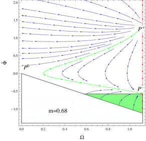
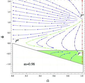
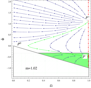
Figure 1: Plot for the phase plane evolution of LRS BI model with $w=1$, $v^{2}=k^{2}=1$, $\zeta_{0}=1$ and different values of $m$. White and green regions represent negativity of entropy production rate and accelerated expansion, respectively.

We find that the green region (accelerated expansion) increases by increasing $m$. For $m=0.68$ and $v^{2}=k^{2}=1$, the point $P_{d}^{-}$ is a global attractor which lies in the physical phase space outside the green region showing decelerated expansion of the universe model dominated by matter. For $m\rightarrow 1$, i.e., $m=0.98,~{}1.02$, it is found that the global attractor $P_{d}^{-}$ lies in the green region showing an expanding model (due to viscosity effects) dominated by matter. The respective analysis is shown in Figure 1. For $v^{2}=k^{2}=0.04$, the graphical results show decelerated expansion coming from both viscous radiation and non-viscous dust for all choices of $m$ (Figure 2). The summary of the results for the stability of LRS BI model filled by dust fluid is given in Table 1.

Table 1: Stability Analysis of Critical Points for Dust Case Critical Point $P^{0}_{d}$ $P^{-}_{d}$ $P^{+}_{d}$ Behavior Saddle Sink Source Stability Unstable Stable Unstable

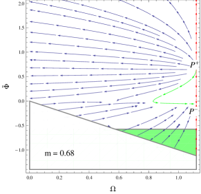
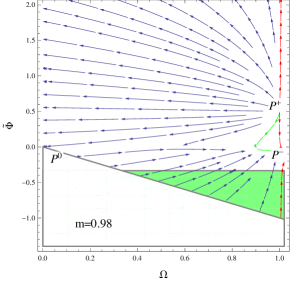
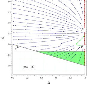
Figure 2: Plot for the phase plane evolution with $w=1$, $v^{2}=k^{2}=0.04$, $\zeta_{0}=1$ and and different values of $m$.

3.2 Radiation Like EoS $(w=\frac{4}{3})$

Here we impose the condition (37) and $\tilde{\Phi}^{\prime}=0$ in Eq.(LABEL:17) which gives a cubic equation of the form

$$\frac{v^{2}}{3\zeta_{0}}\tilde{\Phi}^{3}-\left(m+2+\frac{4v^{2}}{\zeta_{0}}\right)\tilde{\Phi}^{2}+(m+2)(2m+1)\left[\frac{2(2m+1)v^{2}}{\zeta_{0}}\right.$$

$$+\left.\frac{1}{576}\{368m^{2}+1505m+1502\}\right]\tilde{\Phi}+\frac{4v^{2}}{2m+1}-1=0.$$ (44)

This equation provides three roots among which we retain only those roots that lie in the physical phase space. We find two critical points $P_{r}^{+}=\{\frac{3}{m+2},\tilde{\Phi}_{c}^{+}\}$ and $P_{r}^{-}=\{\frac{3}{m+2},\tilde{\Phi}_{c}^{-}\}$ corresponding to positive $(\tilde{\Phi}_{c}^{+})$ and negative $(\tilde{\Phi}_{c}^{-})$ roots, respectively. Using $\tilde{\Phi}^{\prime}=0$ and the second condition (38) with $\tilde{\Phi}_{c}=-\frac{\Omega_{c}}{3}$, we obtain two critical points $P^{0}_{r}=\{0,0\}$ and

$$P^{*}_{r} = \left\{\frac{48v^{2}(m+2)\zeta_{0}}{(2m+1)[128-9(m+2)\zeta_{0}]},-\frac{16v^{2}(m+2)\zeta_{0}}{(2m+1)[128-9(m+2)\zeta_{0}]}\right\},$$

subject to the condition $\Omega_{c}\leq\frac{3}{m+2}$ for their influence in the physical phase space region such that

$$0<v\leq\bar{v},\quad\zeta_{0}>0,\quad\zeta_{0}>\frac{1}{3(m+2)(m+1)^{2}}\bar{\zeta_{0}},$$ (46)

where $\bar{v}=\frac{1}{2(m+2)}\sqrt{\frac{1}{6\zeta_{0}}[3(m+2)(m+1)^{2}\zeta_{0}+\bar{\zeta_{0}}]}$ and $\bar{\zeta_{0}}=\frac{2m+1}{32}$.

The eigenvalues for stability matrix corresponding to the points $P^{\pm}_{r}$ are given by

$$\lambda_{1} = \frac{2}{3}(m+2)\Omega+(m+2)\tilde{\Phi}-1,$$ (47)

$$\lambda_{2} = -\frac{4v^{2}(2m+1)}{3\zeta_{0}(m+2)^{2}[4+(m+2)\tilde{\Phi}]^{2}}-\frac{5(2m+1)}{4}\tilde{\Phi}-\frac{4m+9}{8(m+2)}.$$

In case of viscous radiation like fluid, the location of source and sink can be observed according to the sign of eigenvalues as well as direction of the trajectories. We investigate stability of the critical points corresponding to different values of $m$ and other parameters. For $v=\sqrt{2/3}$ and $0.68$, sink $P_{d}^{-}$ lies in the region with $q>0$ showing decelerated expansion of the universe model (Figure 3). The green region gradually increases by increasing the values of $m$. We find accelerated expansion for more realistic values of parameter $m$ approaching to unity dominated by viscous radiation.

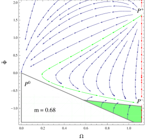
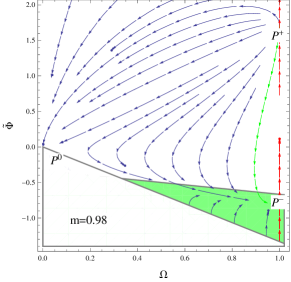
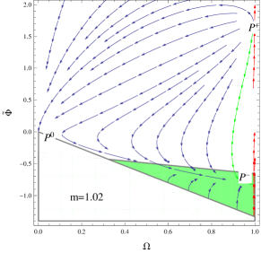
Figure 3: Plot for the phase plane evolution of viscous radiating fluid with $w=4/3$, $v=\sqrt{2/3}$, $\zeta_{0}=1$ and different values of $m$.

The behavior of critical point $P_{r}^{*}$ depends on the condition (46) and the choice of different parameters. If Eq.(46) holds, we observe that the points $P_{r}^{*}$ and $P_{r}^{-}$ are stable attractors for $v=\bar{v}$, $\zeta_{0}=\bar{\zeta_{0}}+1/10$ and different values of $m$. The respective evolution plots are given in Figure 4. It is mentioned here that all choices of parameter $m$ show decelerated expansion of the universe model with contributions coming from both viscous radiation and non-viscous matter. We provide summary of our results filled with viscous radiation like fluid in Table 2.

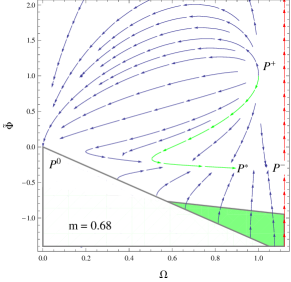
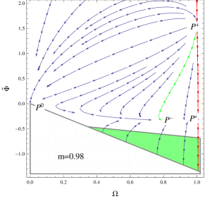
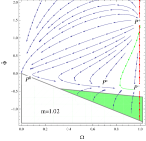
Figure 4: Plot for the phase plane evolution of viscous radiating fluid with $w=4/3$, $v=\bar{v}$, $\zeta_{0}=\bar{\zeta_{0}}+1/10$ and different values of $m$.

Table 2: Stability Analysis of Critical Points for Radiation Dominated Fluid

Critical Point If Eq.(46) holds If Eq.(46) does not hold $P_{r}^{0}$ Saddle Saddle $P_{r}^{+}$ Source Source $P_{r}^{-}$ Sink/Saddle Sink $P_{r}^{*}$ Sink -

Here we also provide a comparison of our results with the work done in literature. Chimento et al. [36] discussed the behavior of homogeneous and isotropic universe model for both barotropic as well as the ideal gas temperature. They investigated asymptotic stability of the de Sitter and Friedmann solutions in which the former is stable for bulk viscosity index having values less than unity and the latter for the values greater than $1$. In our case, we consider barotropic temperature. The bulk viscosity coefficient $\zeta_{0}=1$ as well as smaller values of parameter $m$ show that the stable attractor lies in the region of decelerated expansion showing matter dominated universe followed by viscous radiation. The region for accelerated expansion tends to increase by increasing the values of $m$ such that we investigate accelerated expansion (de Sitter universe) for more realistic values of parameter $m$ approaching to unity. For $\zeta_{0}>1$, we find stability of decelerated expansion of the universe model with contributions coming from both viscous radiation and non-viscous matter for all choices of parameter $m$.

4 Power-Law Scale Factor

In this section, we apply some assumptions on the scale factors corresponding to the critical points. In this way, Eq.(19) yields

$$\dot{\Theta}=-\frac{1}{2}\left[\frac{3}{m+2}+\frac{2m+1}{3}[(w-1)\Omega+\tilde{\Phi}]\right]\Theta^{2}.$$ (49)

For $\Theta\neq 0$, we obtain power-law scale factor whenever $\frac{3}{m+2}+\frac{2m+1}{3}[(w-1)\Omega+\tilde{\Phi}]\neq 0$. Solving $\Theta=\frac{\dot{a}}{a}+\frac{2\dot{b}}{b}$ for $a(t)$ and $b(t)$, we find the corresponding generic critical point as

$$b^{(m+2)}=b_{0}^{(m+2)}(t-t_{0})^{\frac{2}{\frac{3}{m+2}+\frac{2m+1}{3}[(w-1)\Omega_{c}+\tilde{\Phi_{c}}]}}.$$ (50)

For exponentially expanding physical regions, the following condition must be satisfied

$$(1-w)\Omega_{c}-\frac{9}{(m+2)(2m+1)}>-\frac{wv^{2}}{k^{2}}\Omega.$$ (51)

This condition does not hold in the physical phase space for $v^{2}=k^{2}$. If $v^{2}>k^{2}$, the above inequality must be satisfied in the following physical phase space region

$$\frac{9}{(m+2)(2m+1)}\left[1-w\left(1-\frac{v^{2}}{k^{2}}\right)\right]^{-1}<\Omega\leq\frac{3}{m+2}.$$ (52)

It is mentioned here that the sign of the term $\frac{3}{m+2}+\frac{2m+1}{3}[(w-1)\Omega+\tilde{\Phi}]$ is quite important to evaluate different cosmological stages. If $\frac{3}{m+2}+\frac{2m+1}{3}[(w-1)\Omega+\tilde{\Phi}]=0$, it corresponds to the exponential expansion of the universe model. Also, $\frac{3}{m+2}+\frac{2m+1}{3}[(w-1)\Omega+\tilde{\Phi}]\gtrless 0$ yields accelerated expansion or contraction of the cosmological model, respectively. If $v^{2}<k^{2}$, the possibility of having accelerated expansion will narrow down and the green region will disappear from the physical phase space. We plot the respective results for power-law scale factor to explore different phases of the universe model. Figures 5 and 6 show the physical phase space region (above the white region) whereas green and dark gray regions correspond to accelerated expansion and contraction, respectively. For $v^{2}=k^{2}$, we find green region for accelerated expansion which gets larger by increasing $m$. For $v^{2}>k^{2}$, we find both expansion and contraction regions for the cosmological model. In this case, the contraction decreases by increasing $m$ while the green region becomes larger. Table 3 shows the polynomial behavior of power-law scale factors corresponding to different critical points with $\frac{3}{m+2}+\frac{2m+1}{3}[(w-1)\Omega+\tilde{\Phi}]\neq 0$.

Table 3: Power-law Scale Factors for Different Critical Points

Critical Point Scale factors for $w=1$ Scale factors for $w=4/3$ $P^{0}$ $b_{0}^{(m+2)}(t-t_{0})^{\frac{2(m+2)}{3}}$ $b_{0}^{(m+2)}(t-t_{0})^{\frac{2(m+2)}{3}}$ $P^{+}$ $b_{0}^{(m+2)}(t-t_{0})^{\frac{2}{\frac{3}{m+2}+\frac{2m+1}{3}\tilde{\Phi}^{+}_{c}}}$ $b_{0}^{(m+2)}(t-t_{0})^{\frac{2}{\frac{2(m+5)}{3(m+2)}+\tilde{\Phi}^{+}_{c}}}$ $P^{-}$ $b_{0}^{(m+2)}(t-t_{0})^{\frac{2}{\frac{3}{m+2}+\frac{2m+1}{3}\tilde{\Phi}^{-}_{c}}}$ $b_{0}^{(m+2)}(t-t_{0})^{\frac{2}{\frac{2(m+5)}{3(m+2)}+\tilde{\Phi}^{-}_{c}}}$ $P^{*}$ - $b_{0}^{(m+2)}(t-t_{0})^{\frac{2(m+2)}{3}}$

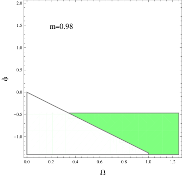
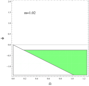
Figure 5: Plot of qualitative phase space analysis for power-law scale factor with $v^{2}=k^{2}$.

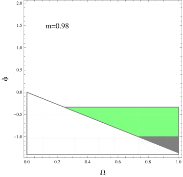
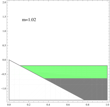
Figure 6: Plot of qualitative phase space analysis for power-law scale factor with $v^{2}>k^{2}$. Green and dark gray regions indicate the accelerated expansion and contraction of the universe model, respectively.

5 Summary

This paper is devoted to study the phase space analysis for LRS BI universe model by taking noninteracting mixture of dust like and viscous radiation like fluids. This analysis has been proved to be a remarkable technique for the study of stability of dynamical system. An autonomous system of equations has been developed by defining normalized dimensionless variables. In order to discuss stability of the system, we have evaluated the corresponding critical points for different values of the parameters. We have also calculated eigenvalues which characterize these critical points. Moreover, we have applied some assumptions on the scale factors to obtain power-law scale factor whose behavior indicates the expansion or contraction of the universe model. We summarize our results as follows.

Firstly, we have discussed stability of critical points through their eigenvalues corresponding to different values of $m$ for pressureless fluid. It is found that the critical points $P^{+}_{d}$ and $P^{-}_{d}$ correspond to source (unstable) and sink (stable), respectively (Figures 1 and 2). The white region shows the universe models with a negative entropy production rate which diverges on its boundary. It is mentioned here that trajectories in its neighborhood are not attracted towards the boundary showing its significant role to keep the models away from divergence. The green region corresponds to the accelerated expansion of the universe. It is found that the point $P_{d}^{-}$ is a global attractor in the physical phase space region which leads to an expanding model dominated by viscous matter for $m$ approaching to unity and $v^{2}=k^{2}=1$ while $m=0.68$ corresponds to deceleration of the respective model. For $v^{2}=k^{2}=0.04$, all choices of $m$ show decelerated expansion dominated by matter.

Secondly, we have studied stability of the critical points in a viscous radiation like fluid. In this case, the critical points $P_{r}^{+}$ and $P_{r}^{-}$ correspond to source and sink, respectively. If Eq.(46) holds, we have found that the behavior of $P_{r}^{-}$ is not fixed rather depends on the values of different parameters. In the case of viscous radiation, we have emphasized on the fact that any trajectory starting from a neighborhood of $P^{+}_{r}$ will go through the following stages in physical phase space region: (i) source $P_{r}^{+}$ corresponds to a radiation dominated era, (ii) saddle $P_{r}^{0}$ showing a matter dominated era, (iii) decelerated expansion (sink $P_{r}^{-}$ or $P_{r}^{*}$). It is found that stable solutions exist for noninteracting fluids in the presence of nonlinear bulk viscosity for $m$ closer to unity which show accelerated expansion of the universe model. If Eq.(46) does not hold, the universe model is in decelerating era for all the choices of $m$. It is worth mentioning here that $m=0.98,~{}1.02$ are more acceptable values for phase space analysis of LRS BI universe model.

We have also obtained power-law scale factor whose behavior indicates expansion or contraction of the universe model for different values of $m$ and the other parameters. Figures 5 and 6 show the physical phase space region (above the white region) whereas green and dark gray regions correspond to accelerated expansion and contraction, respectively. The boundary between green and dark gray regions represents exponential expansion of the universe model. For $v^{2}=k^{2}$, it is found that the green region for accelerated expansion gets larger by increasing $m$. For $v^{2}>k^{2}$, we find both expansion and contraction regions for the respective cosmological model. In this case, the contraction decreases by increasing $m$ while the green region becomes larger. We conclude that our analysis does not provide a complete immune from fine-tuning because the exponentially expanding solution occurs only for a particular range of parameters.

References

- [1] Riess, A.G. et al.: Astron. J. 116(1998)1009; Perlmutter, S.J. et al.: Astrophys. J. 517(1999)565; Bennett, C.L. et al.: Astrophys. J. Suppl. 148(2003)1.
- [2] Sahni, V. and Starobinsky, A.A.: Int. J. Mod. Phys. A 9(2000)373; Tegmark, M. et al.: Phys. Rev. D 69(2004)03501; Copeland, E.J., Sami, M. and Tsujikawa, S.: Int. J. Mod. Phys. D 15(2006)1753.
- [3] Rich, J.: Fundamentals of Cosmology (Springer, 2010).
- [4] Caldwell, R.R., Dave, R. and Steinhardt, P.J.: Phys. Rev. Lett. 80(1998)1582; Chiba, T., Okabe, T., Yamaguchi, M.: Phys. Rev. D 62(2000)023511.
- [5] Carroll, S.M., Hoffman, M. and Trodden, M.: Phys. Rev. D 68(2003)023509.
- [6] Gorini, V. et al.: Phys. Rev. D 69(2004)123512.
- [7] Chimento, L.P.: Phys. Rev. D 69(2004)123517.
- [8] Kamenshchik, A., Moschella, U. and Pasquier, V.: Phys. Lett. B 511(2001)265.
- [9] Bento, M. C., Bertolami, O. and Sen, A.A.: Phys. Rev. D 66(2002)043507.
- [10] Zimdahl, W.: Phys. Rev. D 53(1996)5483.
- [11] Wilson, J.R., Mathews, G.J. and Fuller, G.M.: Phys. Rev. D 75(2007)043521.
- [12] Bogoyavlensky, O.I.: Qualitative Theory of Dynamical System in Astrophysics and Gas Dynamics (Springer, 1985)
- [13] Copeland, E.J., Liddle, A.R. and Wands, D.: Phys. Rev. D 57(1998)4686.
- [14] Guo, Z.K. et al.: Phys. Lett. B 608(2005)177.
- [15] Yang, R.J. and Gao, X.T.: Class. Quantum Grav. 28(2011)065012.
- [16] Xiao, K. and Zhu, J.: Phys. Rev. D 83(2011)083501.
- [17] Acquaviva, G. and Beesham, A.: Phys. Rev. D 90(2014)023503.
- [18] Acquaviva, G. and Beesham, A.: Class. Quantum Grav. 32(2015)215026.
- [19] Sharif, M. and Mumtaz, S.: Eur. Phys. J. C 77(2017)136.
- [20] Eriksen, H.K. et al.: Astrophys. J. 605(2004)14.
- [21] Coley, A.A. and Dunn, K.A.: J. Math. Phys. 33(1992)1772.
- [22] Sharif, M. and Waheed, S.: Astrophys. Space Sci. 351(2014)329.
- [23] Sharif, M. and Jabbar, S.: Commun. Theor. Phys. 63(2015)168.
- [24] Sharif, M. and Mumtaz, S.: Astrophys. Space Sci. 362(2017)205.
- [25] Sharif, M. and Mumtaz, S.: arXiv:1706.07659.
- [26] Sharif, M. and Zubair, M.: Astrophys. Space Sci. 330(2010)399.
- [27] Throne, K. S.: Astrophys. J. 148(1967)51; Collins, C.B., Glass, E.N. and Wilkinson, D.A.: Gen. Relativ. Gravit. 12(1980)805.
- [28] Kantowski, R., Sachs, R. K.: J. Math. Phys. 7(1966)433.
- [29] Collins, C.B.: Phys. Lett. A 60(1977)397.
- [30] Roy, S.R. and Banerjee, S.K. Class. Quantum Grav. 11(1995)1943; Bali, R. and Kumawat, P.: Phys. Lett. B 665(2008)332; Sharif, M. and Waheed, S.: Eur. Phys. J. C 72(2012)1876; Shamir, F.M.: Eur. Phys. J. C 75(2015)354.
- [31] Collins, C.B. and Hawking, S.W.: Astrophys. J. 180(1973)317.
- [32] Campanelli, L. et al.: Phys. Rev. D 83(2011)103503; Kumar, S. and Akarsu, : Eur. Phys. J. Plus 127(2012)64.
- [33] Maartens, R. and Méndez, V.: Phys. Rev. D 55(1997)1937.
- [34] Mohan, N.D.J., Sasidharan, A. and Mathew, T.K.: Eur. Phys. J. C 77(2017)849.
- [35] Maartens, R.: arXiv: astro-ph/9609119v1.
- [36] Chimento, L., Jakubi, A., Mendez, V. and Maartens R.: Class. Quantum Grav. 14(1997)3363.