Formalizing Time4sys using parametric timed automata

Abstract

Critical real-time systems must be verified to avoid the risk of dramatic consequences in case of failure. Thales developed an open formalism “Time4sys” to model real-time systems, with expressive features such as periodic or sporadic tasks, task dependencies, distributed systems, etc. However, Time4sys does not natively allow for a formal reasoning. In this work, we present a translation from Time4sys to (parametric) timed automata, so as to allow for a formal verification.

I Introduction

Real-time systems combine concurrent behaviors with hard real-time constraints. The correctness of real-time systems is crucial especially for critical systems, the failure of which may cause irreparable damages. A formal analysis of the system before its execution is therefore necessary. Real-time systems are made of tasks (that can be periodic or not) to be executed on one or more processors. Tasks are notably characterized by a relative deadline that stipulates how much time can be spent from the activation time of an instance of the task to the completion of that instance. Often, a deadline miss in a real-time system is an undesired behavior just as bad as a wrong result in a computation. Each processor comes with a scheduling policy, that decides what task should be executed. Such policies can be preemptive, i. e., may temporarily stop a task processing to move to a higher priority task. Of utmost importance is the schedulability analysis, that is: given a set of tasks to execute with their timing constraints (period, best case and worst case execution times, deadline) together with the scheduling policies, ensure that no deadline miss will occur.

Thales, a multinational company of 64,000 employees focusing on aerospace, defense and transportation, developed an internal tool for modeling real-time systems. This tool was then recently made public under the name Time4sys, with its code made open source.

Fig. 1 shows an example of Time4sys’ graphical user interface, with one processor (“CPU1”, yellow square) on which 6 tasks (blue squares) are assigned. Blue lines indicate task dependencies: for example, whenever task Trajectory_Prediction is completed, an instance of Tracking_Control2 is activated. Two tasks are periodically activated, i. e., Tracking_Control1 (period: 100 ms, jitter: 30 ms), and Processing (period: 40 ms, no jitter).

However, Time4sys mainly focuses on modeling, and not on verification. While it is possible to design complex real-time systems using Time4sys and its graphical user interface (see Fig. 1), no formal verification can be made. As a consequence, transformation rules from a subset of the Time4sys syntax were proposed to the input format of tools such as Pegase, MAST [Gon+01] or Cheddar [Sin+04], which allow for some formal verification. However, these tools only support some syntactic features: for example, Cheddar does not support task dependency constraints. In 2015, the FMTV challenge made public a problem proposed by Thales, that consists in performing some verifications (and computations) on a real-time system model designed using Time4sys. Due to uncertain periods, i. e., periodic tasks with a fixed but not completely known period, most solutions failed in computing the desired best-case and worst-case computation times. Beside a solution that obtained the correct times using simulation, the only method able to compute these times in an exact fashion used parametric timed model checking [SAL15]. Although modeled by Time4sys, the model of [SAL15] was formalized in an ad-hoc manner to solve a given problem, while we propose here a systematic formalization.

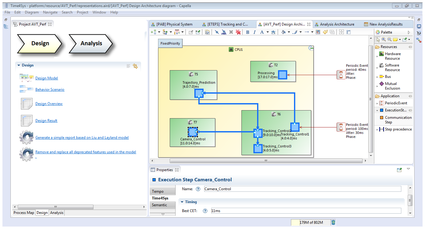
Figure 1: Time4sys graphical user interface

Contribution

In this work, we propose a translation of the Time4sys syntax to an extension of timed automata [AD94], a common formalism to verify systems involving concurrency and time. In addition, we allow the use of parameters to cope for uncertainty by setting as target of our translation parametric timed automata, that extend timed automata with unknown (or uncertain) constants [AHV93]. In other words, some values such as periods or offsets can be completely unknown, or known with a limited certainty (e. g., in a predefined interval). The goal is to offer translation rules, so as to be able to analyze formally Time4sys models even in the presence of uncertainty. Even further, the ultimate goal is to synthesize the values of some timings constants seen as parameters that make the system schedulable.

Related works

Schedulability analysis of real-time systems using model checking was tackled in the past, with several works in the 1990s directly or indirectly targeting real-time systems (e. g., [WME92, AHV93, AD94, YMW97, CC99]). In [AM02, AAM06], schedulability analysis for some real-time systems is performed using timed automata [AD94] or stopwatch automata.

When timing constants (periods, jitters, offsets, deadlines, etc.) become uncertain or unknown, schedulability analysis becomes much harder. A method is to use parametric timed formalisms such as parametric timed automata [AHV93]. In [CPR08] parametric automata are used to synthesize values for offsets, periods, deadlines or computation times for which the system is schedulable. While the problem is in general undecidable, a decidable subclass is exhibited. In [Fri+12], the authors use stopwatch automata to perform robust schedulability analysis, i. e., where some of the timing constants can vary while preserving the schedulability. In [Sun+13], we proposed a method to synthesize values of values such as deadlines and periods for which schedulability is ensured for a real-time system modeled using a set of pipelines: while the method is slower than an analytical method and MAST [Gon+01], our method is also more complete. Despite some ad-hoc experiments, no automatic transformation from an existing formalism to parametric timed automata was proposed.

For uniprocessor real-time systems only, (parametric) task automata offer a more compact representation than (parametric) timed automata [Fer+07, NWY99, And17].

Finally, Time4sys was partially translated to parametric time Petri nets [Lim+09].

Outline

We present Time4sys in Section II. We recall the syntax and semantics of parametric timed automata in Section III. We present our main transformation in Section IV, and we report experiments as a proof of concept in Section V. Finally, we conclude and outline perspectives in Section VI.

II Time4sys

Time4sys is a graphical representation of real-time systems designed and released by Thales.

Time4sys has a formally established syntax given in the form of a metamodel. Time4sys uses a subset of the MARTE OMG standard [OMG08] as a basis to represent a synthetic view of the system design model that captures all elements, data and properties impacting the system timing behavior and required to perform timing verification (e. g., tasks mapping on processors, communication links, execution times, scheduling parameters, etc.).

By using MDE (model-driven engineering) settings, Time4sys is being developed as an Eclipse Polarsys plugin, and comes with a user-friendly graphical interface.

While the semantics of real-time systems modeled in Time4sys is clear (perhaps up to some minor aspects), Time4sys does not natively allow itself for any verification, and relies on external tools such as MAST [Gon+01] or Cheddar [Sin+04].

Figure 2: The beginning of a possible execution of the system in Fig. 3

Supported features

Time4sys allows to model processors (“hardware resources”) and tasks (“software resources”), with their execution times (possibly in the form an interval) and their deadline. In addition, tasks can be activated periodically or sporadically, possibly with a minimum inter-arrival time. Periodic tasks can be subject to a jitter $j$: that is, the $i$th instance of a task with period $p$ will occur in $[(i-1)\times p-j,(i-1)\times p+j]$. In addition, tasks can be subject to an offset $o$: in that case, the $i$th instance of a task with period $p$ will occur at time $(i-1)\times p+o$.

Tasks usually come with a relative deadline: that is, every time a new task instance is activated, this instance must complete its execution within this deadline. Otherwise, a deadline miss occurs, and the system is not schedulable. The schedulability analysis consists in formally checking that, for any execution consistent with the task model (periods, offsets, deadlines, execution times, scheduling policy…), no deadline miss will ever occur.

Time4sys supports both uniprocessor and multi-processor real-time systems. Task dependencies are supported, including between different processors; that is, the completion of a task on a given processor can trigger the activation of a task on the same or on another processor. This is perhaps one of the key aspects of Time4sys, as these dependencies are not always supported by existing schedulability analysis techniques.

Various scheduling policies are supported by Time4sys, including:

• fixed priority ($\mathsf{FPS}$): each task on a given processor comes with a given static priority and, upon completion of a task instance, the highest priority task instance in the waiting queue is selected for execution;

• preemptive $\mathsf{FPS}$: a version of $\mathsf{FPS}$ where a lower priority task can be temporarily stopped to execute a newly activated instance of a higher priority task;

• (preemptive) $\mathsf{RMS}$: $\mathsf{FPS}$ where tasks with shorter periods necessarily have a higher priority;

• shortest job first ($\mathsf{SJF}$): the shortest task instance is selected first;

• Time-division multiple access ($\mathsf{TDMA}$) and Round Robin: tasks are allocated slots in a cyclic manner to execute (part of) their instances, one after the other.

Example 1.

Consider the real-time system in Fig. 3 modeled using Time4sys (the $[0;0]$ intervals should be disregarded). This system features seven tasks to be executed on three processors. Processors are depicted in yellow boxes, while tasks are depicted using blue squares (green boxes can be disregarded in our framework). Blue lines represent task dependencies, while red lines denote sporadic or periodic activations. Tasks $T_{1}$ and $T_{5}$ are periodic, $T_{6}$ is sporadic, while others are activated by task dependencies. Only task $T_{1}$ is subject to an offset (called “phase” in Time4sys). All three processors use the $\mathsf{FPS}$ scheduling policy. Assume that periodic tasks (Task 1 and Task 6) have deadlines equal to their period (i. e., 10 and 20, respectively).

Let us consider the beginning of a possible execution of this system (given in Fig. 2). At system start ($t=0$), Task 5 will be activated; as Task 1 is not activated (due to the offset of 5), Task 5 (although of lower priority) executes on CPU1. On CPU3, Task 6 may be activated anytime, as this is a sporadic task. Let us assume Task 6 is not activated at $t=0$. At $t=0$, no other task is activated and therefore only CPU1 is active, and both CPU2 and CPU3 are idle. At $t=4$, Task 6 is activated, and starts on CPU3. Then, at $t=5$ (which is the offset of Task 1), an instance of Task 1 is activated; as Task 1 has higher priority than Task 5, Task 5 is preempted, and Task 1 starts executing. At $t=9.4$, Task 1 finishes its computation (recall that its computation time lies in $[4,5]$). Then, at that time, an instance of Task 2 is activated by the completion of Task 1; as CPU2 is idle, it starts to execute immediately. In parallel, the computation of Task 5 resumes on CPU1; assuming this execution of Task 5 lasts 7 time units (in interval $[6,8]$), then this instance will be completed at $t=11.4$. At $t=10$, Task 6 completes, triggering the activation of Task 7 on CPU2—which must however wait the end of T2 since it is of lower priority. And so on.

Now observe that, if the deadline of Task 5 was 11 (instead of 20), then at $t=11$, a deadline miss would occur for Task 5, as the execution of its instance is not completed by its deadline (see Section -A1 for details). Or, alternatively, if the deadline of Task 5 was 20 but the worst case execution time of Task 1 was 15, then at $t=20$, Task 5 has still not completed, and again a deadline miss occurs (see Section -A2 for details).

This justifies the study of two problems for Time4sys models:

• being able to verify that a system is schedulable;

• being able to exhibit suitable values (notably for execution times and deadlines) for which the system is schedulable.

III Parametric timed automata

Let ${\mathbb{N}}$, ${\mathbb{Q}}_{+}$ and ${\mathbb{R}}_{\geq 0}$ denote the set of non-negative integers, non-negative rationals and non-negative reals, respectively.

We assume a set $\mathbb{X}=\{x_{1},\dots,x_{H}\}$ of clocks, i. e., real-valued variables that evolve at the same rate. A clock valuation is a function $\nu:\mathbb{X}\rightarrow{\mathbb{R}}_{\geq 0}$. We write $\vec{0}$ for the clock valuation assigning $0$ to all clocks. Given $d\in{\mathbb{R}}_{\geq 0}$, $\nu+d$ denotes the valuation s.t. $(\nu+d)(x)=\nu(x)+d$, for all $x\in\mathbb{X}$. Given $R\subseteq\mathbb{X}$, we define the reset of a valuation $\nu$, denoted by $[\nu]_{R}$, as follows: $[\nu]_{R}(x)=0$ if $x\in R$, and $[\nu]_{R}(x)=\nu(x)$ otherwise.

We assume a set $\mathbb{P}=\{p_{1},\dots,p_{M}\}$ of parameters, i. e., unknown constants. A parameter valuation $v$ is a function $v:\mathbb{P}\rightarrow{\mathbb{Q}}_{+}$. We assume ${\bowtie}\in\{<,\leq,=,\geq,>\}$. A guard $g$ is a constraint over $\mathbb{X}\cup\mathbb{P}$ defined by a conjunction of inequalities of the form $x\bowtie d$, or $x\bowtie p$ with $x\in\mathbb{X}$, $d\in{\mathbb{N}}$ and $p\in\mathbb{P}$. Given $g$, we write $\nu\models v(g)$ if the expression obtained by replacing each $x$ with $\nu(x)$ and each $p$ with $v(p)$ in $g$ evaluates to true.

Parametric timed automata (PTA) extend timed automata [AD94] with parameters within guards and invariants in place of integer constants [AHV93].

Definition 1 (PTA).

A PTA $\mathcal{A}$ is a tuple $\mathcal{A}=(\Sigma,L,l_{0},\mathbb{X},\mathbb{P},I,E)$, where:

1. $\Sigma$ is a finite set of synchronization actions,

2. $L$ is a finite set of locations,

3. $l_{0}\in L$ is the initial location,

4. $\mathbb{X}$ is a finite set of clocks,

5. $\mathbb{P}$ is a finite set of parameters,

6. $I$ is the invariant, assigning to every $l\in L$ a guard $I(l)$,

7. $E$ is a finite set of edges $e=(l,g,a,R,l^{\prime})$ where $l,l^{\prime}\in L$ are the source and target locations, $a\in\Sigma$, $R\subseteq\mathbb{X}$ is a set of clocks to be reset, and $g$ is a guard.

Given a parameter valuation $v$, we denote by $v(\mathcal{A})$ the non-parametric structure where all occurrences of a parameter $p_{i}$ have been replaced by $v(p_{i})$. We denote as a timed automaton any structure $v(\mathcal{A})$, by assuming a rescaling of the constants: by multiplying all constants in $v(\mathcal{A})$ by their least common denominator, we obtain an equivalent (integer-valued) TA, as defined in [AD94].

Example 2.

An example of PTA is given in Fig. 4(a) (page 4(a)). It features two locations ${\color[rgb]{0.2,0.2,0.35}\mathrm{l1}}$ and ${\color[rgb]{0.2,0.2,0.35}\mathrm{l2}}$, one synchronization action ${\color[rgb]{0.50,0.70,0.30}\mathrm{actT}}$, one clock ${\color[rgb]{0.4,0.4,1}\mathrm{xactT}}$, and two parameters ${\color[rgb]{1,0.6,0.0}\mathrm{TPeriod}}$ and ${\color[rgb]{1,0.6,0.0}\mathrm{TOffset}}$.

Let us now recall the concrete semantics of TA.

Definition 2 (Semantics of a TA).

Given a PTA $\mathcal{A}=(\Sigma,L,l_{0},\mathbb{X},\mathbb{P},I,E)$, and a parameter valuation $v$, the semantics of $v(\mathcal{A})$ is given by the timed transition system (TTS) $(S,s_{0},{\rightarrow})$, with

• $S=\{(l,\nu)\in L\times{\mathbb{R}}_{\geq 0}^{H}\mid\nu\models v(I(l))\}$,

• $s_{0}=(l_{0},\vec{0})$,

• ${\rightarrow}$ consists of the discrete and (continuous) delay transition relations:

  1. discrete transitions: $(l,\nu)\stackrel{{\scriptstyle e}}{{\mapsto}}(l^{\prime},\nu^{\prime})$, if $(l,\nu),(l^{\prime},\nu^{\prime})\in S$, and there exists $e=(l,g,a,R,l^{\prime})\in E$, such that $\nu^{\prime}=[\nu]_{R}$, and $\nu\models v(g$).

  2. delay transitions: $(l,\nu)\stackrel{{\scriptstyle d}}{{\mapsto}}(l,\nu+d)$, with $d\in{\mathbb{R}}_{\geq 0}$, if $\forall d^{\prime}\in[0,d],(l,\nu+d^{\prime})\in S$.

Given a TA $v(\mathcal{A})$ with concrete semantics $(S,s_{0},{\rightarrow})$, we refer to the states of $S$ as the concrete states of $v(\mathcal{A})$. A run of $v(\mathcal{A})$ is an alternating sequence of concrete states of $v(\mathcal{A})$ and pairs of edges and delays starting from the initial state $s_{0}$ of the form $s_{0},(e_{0},d_{0}),s_{1},\cdots$ with $i=0,1,\dots$, $e_{i}\in E$, $d_{i}\in{\mathbb{R}}_{\geq 0}$ and $(s_{i},e_{i},s_{i+1})\in{\rightarrow}$. Given a state $s=(l,\nu)$, we say that $s$ is reachable in $v(\mathcal{A})$ if $s$ appears in a run of $v(\mathcal{A})$. By extension, we say that $l$ is reachable; and by extension again, given a set $T$ of locations, we say that $T$ is reachable if there exists $l\in T$ such that $l$ is reachable in $v(\mathcal{A})$.

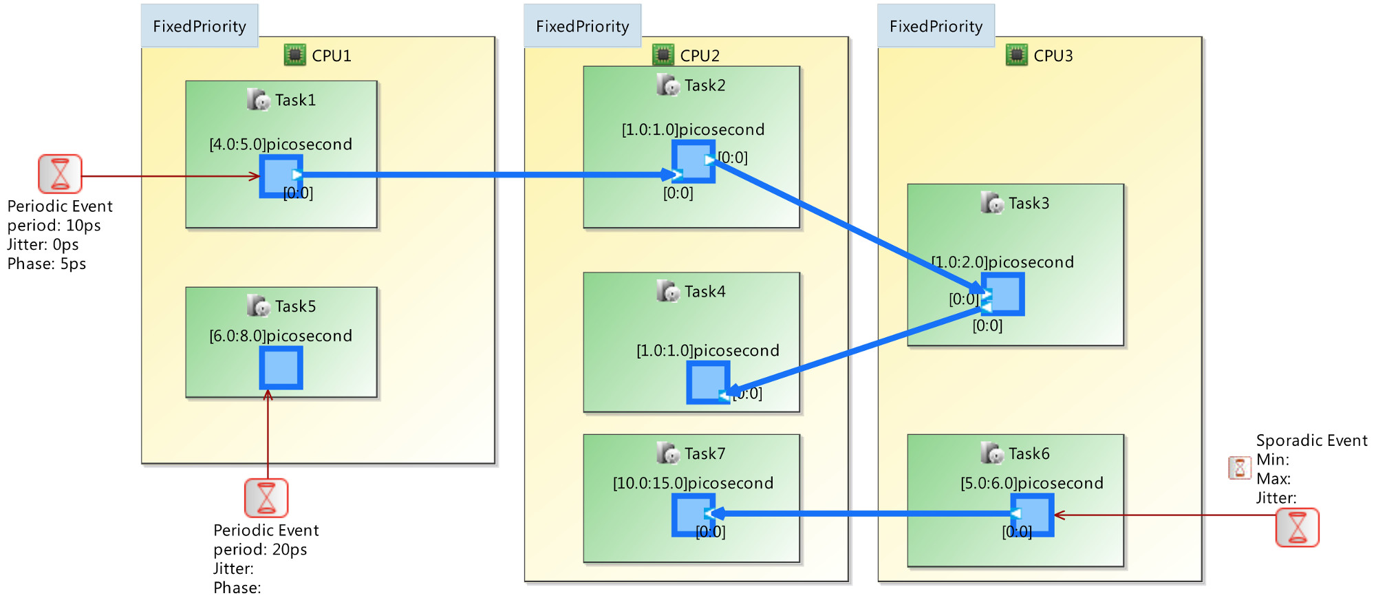
Figure 3: Example of Time4sys model

III-A Reachability synthesis

We will use here reachability synthesis to perform parametric schedulability analysis. That is, the system will be schedulable for valuations of the PTA for which the valuated TA does not reach a set of given locations modeling deadline misses.

The procedure synthesizing valuations for which a set of locations is (un)reachable is called EFsynth: it takes as input a PTA $\mathcal{A}$ and a set of target locations $T$, and attempts to synthesize all parameter valuations $v$ for which $T$ is reachable in $v(\mathcal{A})$. EFsynth was given and formalized in e. g., [JLR15] and may not terminate, but if it terminates, then its result is exact (sound and complete). EFsynth traverses the parametric zone graph of $\mathcal{A}$, which is a potentially infinite extension of the well-known zone graph of TAs (see, e. g., [AS13, JLR15] for a formal definition).

III-B IMITATOR

IMITATOR [And+12] is a parametric timed model checker supporting networks of parametric timed automata extended with various features such as stopwatches (i. e., the ability to stop the elapsing of some clocks, allowing to model preemption in real-time systems), synchronization using synchronization actions, global discrete rational-valued variables that can read and modified in guards, etc. In the following, we refer to these extended PTAs as PTAs. Our translation takes advantage of the features offered by IMITATOR, notably stopwatches and action synchronization.

IMITATOR was used in the past to verify several industrial case studies (e. g., [Fri+12, SAL15]).

IV Translating Time4sys into PTAs

In this section, we present our translation from the syntax of Time4sys into parametric timed automata (extended with stopwatches). We use the real-time system in Fig. 3 to exemplify our translation.

IV-A Assumptions

We make the following assumptions on the Time4sys models we aim at analyzing:

1. We allow only one-to-one task dependencies; that is, a given task upon completion can activate only a single task. This is not the case of Fig. 1 as Tracking_control2 activates two tasks; in contrast, this assumption is satisfied in Fig. 3.

2. For periodic tasks, the deadline is equal to the period.

3. No jitters are allowed.

How to lift these assumptions is discussed in Section VI.

IV-B General translation scheme

We will build a network of PTAs synchronized on synchronization actions. By default, we assume the model is fully parameterized, i. e., all timing constants (deadlines, periods, offsets, jitters…) are parameters in the sense of PTAs’ unknown constants. Assigning these parameters to a fixed value can be done trivially in IMITATOR, and makes the subsequent analysis simpler. For example, in Fig. 3, we should set ${\color[rgb]{1,0.6,0.0}\mathrm{T1period}}:=10\,ps$.

In addition, we use the following same convention as in the literature, as well as in IMITATOR: different objects (clocks, parameters, variables, actions—but not locations) with the same name in different PTAs refer to shared objects. For example, a clock named $x$ used in two different PTAs is the same clock. However, two locations $l_{1}$ in two different PTAs are (naturally) two different locations.

The various PTAs will be synchronized using synchronization actions. Given a task $T$, two actions will be used: ${\color[rgb]{0.50,0.70,0.30}\mathrm{actT}}$, denoting the activation of an instance of $T$, and ${\color[rgb]{0.50,0.70,0.30}\mathrm{finT}}$ to denote its completion. Note that, thanks to our assumption of deadlines equal to periods, not more than one instance of a task is present (executing or waiting) at a given time: indeed, if a second instance of a task is activated, this would mean that the first one did not complete within its period.

IV-C Task activation patterns

We consider two main kinds of activation patterns: periodic tasks and sporadic tasks.

Periodic tasks

Given a task $T$ with period ${\color[rgb]{1,0.6,0.0}\mathrm{TPeriod}}$ and offset ${\color[rgb]{1,0.6,0.0}\mathrm{TOffset}}$, we create a PTA with a local clock ${\color[rgb]{0.4,0.4,1}\mathrm{xactT}}$ synchronizing on action ${\color[rgb]{0.50,0.70,0.30}\mathrm{actT}}$, given in Fig. 4(a). The first location is used to encode the offset at the beginning, while the second one is used to encode the periodic behavior. Initially, in ${\color[rgb]{0.2,0.2,0.35}\mathrm{l1}}$, the system must wait ${\color[rgb]{1,0.6,0.0}\mathrm{TOffset}}$ time units before starting the periodic behavior, according to the definition of the offset. Then, after exactly ${\color[rgb]{1,0.6,0.0}\mathrm{TOffset}}$ time units (encoded by the guard ${\color[rgb]{0.4,0.4,1}\mathrm{xactT}}={\color[rgb]{1,0.6,0.0}\mathrm{TOffset}}$), the PTA activates task $T$ using the synchronization action ${\color[rgb]{0.50,0.70,0.30}\mathrm{actT}}$ and moves to the second location. There, every exactly ${\color[rgb]{1,0.6,0.0}\mathrm{TPeriod}}$ time units (encoded by the guard ${\color[rgb]{0.4,0.4,1}\mathrm{xactT}}={\color[rgb]{1,0.6,0.0}\mathrm{TPeriod}}$), the PTA activates task $T$.

(a) Periodic task

(b) Sporadic task

Figure 4: Translating activation patterns

Sporadic tasks

Sporadic tasks are characterized by their minimum inter-arrival time. The encoding of sporadic task $T$ with minimum inter-arrival time ${\color[rgb]{1,0.6,0.0}\mathrm{TIAT}}$ is very similar to the case of a periodic task, and is given in Fig. 4(b). The only differences are the absence of invariant in the lower location, and the fact that the activation is not anymore when ${\color[rgb]{0.4,0.4,1}\mathrm{xactT}}={\color[rgb]{1,0.6,0.0}\mathrm{TPeriod}}$, but when ${\color[rgb]{0.4,0.4,1}\mathrm{xactT}}\geq{\color[rgb]{1,0.6,0.0}\mathrm{TIAT}}$.

IV-D Task precedences

We now encode task precedences. Recall that, although this syntactic feature is intuitive (“upon completion, a given task triggers the activation of another task”), many tools do not support them; for example, Cheddar does not support task such dependency constraints. Due to our assumption banning multiple precedences, such task precedences can be seen as task chains, that are reminiscent of the pipelines that we modeled in [Sun+13] using PTAs. For example, in Fig. 3, there are three task chains:

1. $T_{1}\rightarrow T_{2}\rightarrow T_{3}\rightarrow T_{4}$;

2. $T_{6}\rightarrow T_{7}$; and

3. $T_{5}$.

Translating these task chains is done by constraining the order between the various task activations and completions. However, since the total execution time of the whole task chain can be larger than the first task’s period, a single automaton is not sufficient. Therefore, we “split” the chain, and encode each dependency as a PTA; as usual, these PTAs will be synchronized on the synchronization actions.

(a) Tasks $T_{1}$ and $T_{2}$

(b) Tasks $T_{2}$ and $T_{3}$

(c) Tasks $T_{3}$ and $T_{4}$

Figure 5: Translating task chain $T_{1}\rightarrow T_{2}\rightarrow T_{3}\rightarrow T_{4}$

We give the translation of the task chain “$T_{1}\rightarrow T_{2}\rightarrow T_{3}\rightarrow T_{4}$” in the three PTAs given in Fig. 5. The three locations named ${\color[rgb]{0.2,0.2,0.35}\mathrm{l3}}$ are urgent locations (preceded by “${\color[rgb]{0.2,0.2,0.35}\mathrm{U:}}$”), i. e., locations where time cannot elapse: that is, in Fig. 5(a), the activation of task $T_{2}$ comes immediately after the completion of $T_{1}$.

IV-E Scheduling policies

The scheduler of each CPU is translated into a PTA according to its scheduling policy. We focus on preemptive $\mathsf{FPS}$ as this is one of the most widely used policies, and arguably one of the most complex to encode. Recall that $\mathsf{FPS}$ always executes the highest priority task (all tasks of a given processor have a different priority); preemption allows to stop the ongoing computation to move to a higher priority incoming task. $\mathsf{RMS}$ is a particular case of $\mathsf{FPS}$ where a shorter period is necessarily assigned a higher priority (not necessarily the case in $\mathsf{FPS}$).

Encoding $\mathsf{FPS}$

Our encoding of $\mathsf{FPS}$ is a formalization of the ad-hoc scheme of [Sun+13]. Fig. 6 shows the translation of CPU1 from Fig. 3, assuming its policy is preemptive $\mathsf{FPS}$, with the priority of Task 1 being higher than that of Task 5. We use stopwatches, and the stopped clocks in a location are given in the dashed rectangle together with the invariant. We assume task $T_{1}$ has higher priority over $T_{5}$. The processor starts by being ${\color[rgb]{0.2,0.2,0.35}\mathrm{idle}}$, waiting for a task activation. As soon as a task is activated (e. g., action ${\color[rgb]{0.50,0.70,0.30}\mathrm{actT5}}$), it moves to one of the locations where the corresponding task is running (${\color[rgb]{0.2,0.2,0.35}\mathrm{execT5}}$). If it receives another activation request (${\color[rgb]{0.50,0.70,0.30}\mathrm{actT1}}$), it moves to the location corresponding to the higher priority task running (${\color[rgb]{0.50,0.70,0.30}\mathrm{execT1waitT5}}$), where $T_{1}$ is executed and $T_{5}$ is waiting to be executed. The fact that $T_{5}$ does not execute anymore is modeled by the stopping of the clock ${\color[rgb]{0.4,0.4,1}\mathrm{xexecT5}}$ corresponding to task $T_{5}$. Moreover, while a task executes, the scheduler automaton checks if it misses its deadline (e. g., guard ${\color[rgb]{0.4,0.4,1}\mathrm{xactT5}}>{\color[rgb]{1,0.6,0.0}\mathrm{T5Period}}$, where ${\color[rgb]{1,0.6,0.0}\mathrm{T5Period}}$ is $T_{5}$’s deadline since we assumed deadlines to be equal to periods). In the case of a deadline miss, the processor PTA moves to a special failure location (“deadline missed”) and stops any further computation.

The model of a non-preemptive processor is very similar to the model of preemptive processor: the central location in Fig. 6 which accounts for the fact that $T_{5}$ is stopped when $T_{1}$ is activated, in the non-preemptive case must not stop $T_{5}$, but simply remember that $T_{1}$ has been released, so that we can move to the top state when $T_{5}$ completes its instance.

Figure 6: Translating the scheduler CPU1 with a preemptive $\mathsf{FPS}$ scheduling policy

Encoding $\mathsf{TDMA}$

We also encoded the “Time-division multiple access” ($\mathsf{TDMA}$) scheduling policy. This scheduling policy is fairly simple, as there are no priorities: the scheduler simply passes a “token” to each of its tasks in a circular manner. If an instance of this task is activated, then this task executed for a predefined amount of time (generally small). If no instance of this task is activated, then the processor remains idle during the predefined amount of time, before moving to the next task.

Other scheduling policies

Other scheduling policies are discussed in Section VI.

IV-F Handling uncertainty

A major interest of our transformation is its ability to handle uncertainty. Indeed, all timing constants (periods, deadlines, offsets…) can be possibly kept parametric, or can be constrained to belong to a predefined interval. For example, to model the period of a task $T_{1}$ equal to 100 ms known with a precision of 1 %, it suffices to declare the parameter ${\color[rgb]{1,0.6,0.0}\mathrm{T1Period}}\in[99,101]$, which can be simulated by a small PTA gadget—or is natively offered by the input syntax of IMITATOR.

Then, the system is schedulable for all valuations such that the system reaches none of the ${\color[rgb]{0.2,0.2,0.35}\mathrm{DeadlineMissed}}$ locations defined in Section IV-E. This can be computed by the EFsynth algorithm implemented in IMITATOR.

IV-G Implementation

We implemented our translation in a Java program of 2,900 lines of code called Time4sys2IMITATOR [AJM19]. The program takes as input a Time4sys model exported from the interface (that comes in the form of an XML file), and outputs a PTA model in the IMITATOR input syntax. We support all the features mentioned in Section IV.

V Experiments

As a proof of concept, we apply our transformation to the example in Fig. 3. Task 1 (resp. 5) has an activation period of 10 (resp. 20) and an offset of 5 (resp. 0). Task 6 is sporadic with a minimum interarrival time of 20. The best and worst case computation times for the tasks are given in bracket; for example, the computation time of each instance of task 1 is non-deterministically chosen in $[4,5]$. Recall that all three processors use $\mathsf{FPS}$. The priorities are chosen as follows: for CPU1, $T1>T5$; for CPU2, $T2>T4>T7$; for CPU2, $T6>T3$.

Our translation yields a model made of 14 synchronization actions, 14 clock variables, and (up to) 28 parameters, that consist of all periods, deadlines, offsets and best and worst case execution times. IMITATOR allows to keep none, some or all of the parameters unconstrained to allow for various levels of parameterization.

Experiments were conducted using IMITATOR 2.10.4 “Butter Jellyfish” on a Dell XPS 13 9365 i7 (2017) running Linux Mint 18.2 64 bits with 8 GiB memory.

Non-parametric schedulability analysis

First, we valuate all parameters (therefore the model is entirely non-parametric), and we assume that all deadlines are equal to period for periodic tasks (we are not interested in deadline violations for other tasks, therefore their deadline can be set to an arbitrarily large value). An analysis with IMITATOR (computation time: 0.2 s) certifies that this model is schedulable, i. e., no deadline miss occurs.

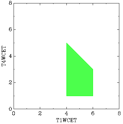
(a) WCET 1 and 4

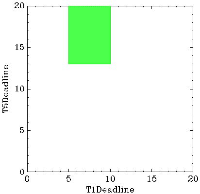
(b) Deadlines 1 and 5

Figure 7: Some 2-D graphical representations

Parametric WCETs

Then, we leave some parameters unconstrained, so as to not only verify the schedulability but also to synthesize parameter values for which the system is schedulable. Leaving ${\color[rgb]{1,0.6,0.0}\mathrm{T1WCET}}$ and ${\color[rgb]{1,0.6,0.0}\mathrm{T4WCET}}$ unconstrained yields the following constraint (time: 1.5s):

$4\leq{\color[rgb]{1,0.6,0.0}\mathrm{T1WCET}}\leq 6\land{\color[rgb]{1,0.6,0.0}\mathrm{T4WCET}}\geq 1\\ \land{\color[rgb]{1,0.6,0.0}\mathrm{T1WCET}}+{\color[rgb]{1,0.6,0.0}\mathrm{T4WCET}}<9$

A graphical representation (output by IMITATOR) is given in Fig. 7(a).

Then, we run a 4-dimensional analysis to infer values for ${\color[rgb]{1,0.6,0.0}\mathrm{T1WCET}}$, ${\color[rgb]{1,0.6,0.0}\mathrm{T4WCET}}$, ${\color[rgb]{1,0.6,0.0}\mathrm{T5WCET}}$ and ${\color[rgb]{1,0.6,0.0}\mathrm{T7WCET}}$ (time: 11.5s); the result is given in Fig. 8(a).

${\color[rgb]{1,0.6,0.0}\mathrm{T5WCET}}\geq 6\land{\color[rgb]{1,0.6,0.0}\mathrm{T4WCET}}\geq 1\\ \land 20\geq 2*{\color[rgb]{1,0.6,0.0}\mathrm{T1WCET}}+{\color[rgb]{1,0.6,0.0}\mathrm{T5WCET}}\\ \land 9>{\color[rgb]{1,0.6,0.0}\mathrm{T1WCET}}+{\color[rgb]{1,0.6,0.0}\mathrm{T4WCET}}\\ \land{\color[rgb]{1,0.6,0.0}\mathrm{T1WCET}}\geq 4\land{\color[rgb]{1,0.6,0.0}\mathrm{T7WCET}}\geq 10\\ \lor\\ {\color[rgb]{1,0.6,0.0}\mathrm{T5WCET}}\geq 6\land{\color[rgb]{1,0.6,0.0}\mathrm{T7WCET}}\geq 10\\ \land 16>2*{\color[rgb]{1,0.6,0.0}\mathrm{T4WCET}}+{\color[rgb]{1,0.6,0.0}\mathrm{T7WCET}}\\ \land{\color[rgb]{1,0.6,0.0}\mathrm{T1WCET}}+{\color[rgb]{1,0.6,0.0}\mathrm{T4WCET}}\geq 9\\ \land 20\geq 2*{\color[rgb]{1,0.6,0.0}\mathrm{T1WCET}}+{\color[rgb]{1,0.6,0.0}\mathrm{T5WCET}}$

(a) 4-dimensional parametric WCETs

${\color[rgb]{1,0.6,0.0}\mathrm{T5Deadline}}\geq{\color[rgb]{1,0.6,0.0}\mathrm{T1WCET}}+{\color[rgb]{1,0.6,0.0}\mathrm{T5WCET}}\\ \land{\color[rgb]{1,0.6,0.0}\mathrm{T1WCET}}\geq 4\\ \land{\color[rgb]{1,0.6,0.0}\mathrm{T1Deadline}}\geq{\color[rgb]{1,0.6,0.0}\mathrm{T1WCET}}\\ \land 15\geq{\color[rgb]{1,0.6,0.0}\mathrm{T1WCET}}+{\color[rgb]{1,0.6,0.0}\mathrm{T5WCET}}\\ \land{\color[rgb]{1,0.6,0.0}\mathrm{T5Deadline}}+5\geq 2*{\color[rgb]{1,0.6,0.0}\mathrm{T1WCET}}+{\color[rgb]{1,0.6,0.0}\mathrm{T5WCET}}\\ \land 20\geq{\color[rgb]{1,0.6,0.0}\mathrm{T5Deadline}}\\ \land 10\geq{\color[rgb]{1,0.6,0.0}\mathrm{T1Deadline}}\\ \land{\color[rgb]{1,0.6,0.0}\mathrm{T5WCET}}\geq 6\\ \land 20\geq 2*{\color[rgb]{1,0.6,0.0}\mathrm{T1WCET}}+{\color[rgb]{1,0.6,0.0}\mathrm{T5WCET}}\\ \lor\\ 10\geq{\color[rgb]{1,0.6,0.0}\mathrm{T1Deadline}}\land{\color[rgb]{1,0.6,0.0}\mathrm{T1Deadline}}\geq{\color[rgb]{1,0.6,0.0}\mathrm{T1WCET}}\\ \land{\color[rgb]{1,0.6,0.0}\mathrm{T1WCET}}+{\color[rgb]{1,0.6,0.0}\mathrm{T5WCET}}>15\\ \land{\color[rgb]{1,0.6,0.0}\mathrm{T1WCET}}\geq 4\\ \land{\color[rgb]{1,0.6,0.0}\mathrm{T5Deadline}}\geq 2*{\color[rgb]{1,0.6,0.0}\mathrm{T1WCET}}+{\color[rgb]{1,0.6,0.0}\mathrm{T5WCET}}\\ \land 20\geq{\color[rgb]{1,0.6,0.0}\mathrm{T5Deadline}}$

(b) WCETs and deadlines

$13>{\color[rgb]{1,0.6,0.0}\mathrm{T1WCET}}+{\color[rgb]{1,0.6,0.0}\mathrm{T1Offset}}\\ \land 6>{\color[rgb]{1,0.6,0.0}\mathrm{T1WCET}}\geq 4\\ \land 10\geq{\color[rgb]{1,0.6,0.0}\mathrm{Deadline}}\\ \land{\color[rgb]{1,0.6,0.0}\mathrm{Deadline}}\geq{\color[rgb]{1,0.6,0.0}\mathrm{T1WCET}}\\ \land{\color[rgb]{1,0.6,0.0}\mathrm{T1Offset}}>1\\ \lor\\ 7>{\color[rgb]{1,0.6,0.0}\mathrm{T1Offset}}>3\\ \land 10\geq{\color[rgb]{1,0.6,0.0}\mathrm{Deadline}}\geq 6\\ \land{\color[rgb]{1,0.6,0.0}\mathrm{T1WCET}}=6$

(c) Task 1: offset, WCET, deadline

Figure 8: Results

Parametric deadlines

We then parameterize deadlines of tasks 1 and 5. The result (computed in 0.63 s) is given below:

${\color[rgb]{1,0.6,0.0}\mathrm{T1Deadline}}\in[5,13]\land{\color[rgb]{1,0.6,0.0}\mathrm{T5Deadline}}\in[10,20]$

A graphical representation is given in Fig. 7(b).

Parametric offset

We also study the influence of the offset of Task 1 on the schedulability. An analysis with one parameter ${\color[rgb]{1,0.6,0.0}\mathrm{OffsetT1}}$ gives (time: 2.0 s): ${\color[rgb]{1,0.6,0.0}\mathrm{OffsetT1}}\in(1,8)$.

It may be surprising that the system is non-schedulable for a zero-offset: this comes from the fact that, if Task 1 is activated too soon, Task 2 (that is activated upon completion of Task 1) will preempt CPU2, preventing Task 7 to complete, notably in the worst case when Task 6 is activated at the highest possible period allowed by its sporadic nature and Task 7 lasts for its longest duration (15 time units).

Multidimensional parametric analyses

We finally relate the various variables of the system by performing parametric analyses in different dimensions. We first relate deadlines and WCETs of tasks 1 and 5. The analysis (time: 8.9 s) gives the result in Fig. 8(b).

Finally, we relate three values of task 1, i. e., its offset, its WCET and its deadline. We give the result (time: 40.6 s) in Fig. 8(c).

VI Perspectives

In this work, we proposed a first translation of an industrial formalism to model real-time systems into a parametric timed formalism, namely parametric timed automata. We discuss below short-term perspectives.

Lifting assumptions

We did not support the full syntax of Time4sys, as we used some assumptions defined in Section IV-A.

We assumed that all periodic tasks must have a deadline equal to the period. While deadlines less than or equal to the period is very straightforward (and is part of our implementation), deadlines larger than periods may render the translation more elaborate. Indeed, our encoding of Section IV-D needs to be deeply modified, as we need to encode more than one instance of a task at a given time. An option is to split further the task chains, and add some additional integer-valued variables, but this solution will come at the cost of a less efficient analysis.

Multiple dependencies remain to be supported: on the one hand, a task activating several tasks (e. g., in Fig. 1, Tracking_control2 upon completion activates both Camera_control and Tracking_control3) is natural and should be supported without difficulties by action synchronization in parametric timed automata; on the other hand, the semantics of several tasks activating a single task looks more dubious, and we are not even sure to want to support this syntax.

Jitters can easily be supported: however, they slightly complicate the model of task activation patterns, and are therefore discarded both in this work and temporarily in our implementation (with the goal to introduce them soon).

After lifting these assumptions, we note that we support the vast majority of the Time4sys syntax, with the exception of multiple input task activation—which, again, may seem dubious as its semantics is very unclear.

Alternative scheduler models

A natural future work will be to propose optimizations or variants in the translation, notably of the scheduler model, and test their practical efficiency on a set of benchmarks, such as the IMITATOR benchmarks library [And19].

Implementing other scheduling policies, such as earliest deadline first ($\mathsf{EDF}$) or shortest job first ($\mathsf{SJF}$), should be straightforward. Round Robin resembles $\mathsf{TDMA}$ in the sense that the scheduler moves a “token” to its tasks; however, the main difference is that, whenever a task has no activated instance, the processor immediately moves to the next one. This is not difficult as such, but this requires more locations in the PTA model than for $\mathsf{TDMA}$.

Translation to Uppaal

A translation into the state-of-the-art Uppaal model-checker [LPY97] is on our agenda. However, a translation to Uppaal would lose the ability to use unknown or uncertain constants; in addition, Uppaal does not fully support stopwatches, needed to model preemption.

Execution traces

Finally, in case of a deadline miss, we aim at displaying the faulty model trace leading to the deadline miss back to the Time4sys model. Note that Time4sys also features a metamodel for such traces.

-A Examples with deadline misses

-A1 Modifying the deadline

Consider again the real-time system in Fig. 3. Now observe that, if the deadline of Task 5 was 11 (instead of 20), then at $t=11$, a deadline miss would occur for Task 5, as the execution of its instance is not completed by its deadline. This situation is depicted in Fig. 9(a): the deadline is depicted using a down arrow, and the part of the execution of the instance of Task 5 violating the deadline is highlighted using a red box.

(a) Deadline miss for Fig. 3 if ${\color[rgb]{1,0.6,0.0}\mathrm{T5Deadline}}=11$

(b) Deadline miss for Fig. 3 if ${\color[rgb]{1,0.6,0.0}\mathrm{T1WCET}}=15$

Figure 9: Two examples of deadline misses

-A2 Modifying the WCET

Alternatively, if the deadline of Task 5 was 20 as in the original definition but the worst case execution time of Task 1 was 15 (with an increased period and deadline for Task 1 of, say, 20), then at $t=20$, Task 5 has still not completed and, again, a deadline miss occurs. This situation is depicted in Fig. 9(b).

References

- [AAM06] Yasmina Adbeddaïm, Eugene Asarin and Oded Maler “Scheduling with timed automata” In Theoretical Computer Science 354.2 Elsevier Science, 2006, pp. 272–300 DOI: 10.1016/j.tcs.2005.11.018
- [AD94] Rajeev Alur and David L. Dill “A theory of timed automata” In Theoretical Computer Science 126.2 Essex, UK: Elsevier Science Publishers Ltd., 1994, pp. 183–235 DOI: 10.1016/0304-3975(94)90010-8
- [AHV93] Rajeev Alur, Thomas A. Henzinger and Moshe Y. Vardi “Parametric real-time reasoning” In STOC San Diego, California, United States: ACM, 1993, pp. 592–601 DOI: 10.1145/167088.167242
- [AJM19] Étienne André, Jawher Jerray and Sahar Mhiri “Time4sys2IMITATOR: A tool to formalize real-time system models under uncertainty”, Submitted, 2019
- [AM02] Yasmina Adbeddaïm and Oded Maler “Preemptive Job-Shop Scheduling using Stopwatch Automata” In TACAS 2280, Lecture Notes in Computer Science Grenoble, France: Springer-Verlag, 2002, pp. 113–126 DOI: 10.1007/3-540-46002-0˙9
- [And+12] Étienne André, Laurent Fribourg, Ulrich Kühne and Romain Soulat “IMITATOR 2.5: A Tool for Analyzing Robustness in Scheduling Problems” In FM 7436, Lecture Notes in Computer Science Paris, France: Springer, 2012, pp. 33–36 DOI: 10.1007/978-3-642-32759-9˙6
- [And17] Étienne André “A unified formalism for monoprocessor schedulability analysis under uncertainty” In FMICS-AVoCS 10471, Lecture Notes in Computer Science Torino, Italy: Springer, 2017, pp. 100–115 DOI: 10.1007/978-3-319-67113-0˙7
- [And19] Étienne André “A benchmark library for parametric timed model checking” In FTSCS 1008, Communications in Computer and Information Science Gold Coast, Australia: Springer, 2019, pp. 75–83 DOI: 10.1007/978-3-030-12988-0˙5
- [AS13] Étienne André and Romain Soulat “The Inverse Method” 176 pages, FOCUS Series in Computer Engineering and Information Technology ISTE LtdJohn Wiley & Sons Inc., 2013
- [CC99] Sérgio Vale Aguiar Campos and Edmund M. Clarke “Analysis and Verification of Real-Time Systems Using Quantitative Symbolic Algorithms” In International Journal on Software Tools for Technology Transfer 2.3, 1999, pp. 260–269 DOI: 10.1007/s100090050033
- [CPR08] Alessandro Cimatti, Luigi Palopoli and Yusi Ramadian “Symbolic Computation of Schedulability Regions Using Parametric Timed Automata” In RTSS Barcelona, Spain: IEEE Computer Society, 2008, pp. 80–89 DOI: 10.1109/RTSS.2008.36
- [Fer+07] Elena Fersman, Pavel Krcál, Paul Pettersson and Wang Yi “Task automata: Schedulability, decidability and undecidability” In Information and Computation 205.8, 2007, pp. 1149–1172 DOI: 10.1016/j.ic.2007.01.009
- [Fri+12] Laurent Fribourg, David Lesens, Pierre Moro and Romain Soulat “Robustness Analysis for Scheduling Problems using the Inverse Method” In TIME Leicester, UK: IEEE Computer Society Press, 2012, pp. 73–80 DOI: 10.1109/TIME.2012.10
- [Gon+01] Michael González Harbour, J.. Gutiérrez García, José C. Palencia Gutiérrez and J.. Drake Moyano “MAST: Modeling and Analysis Suite for Real Time Applications” In ECRTS Delft, The Netherlands: IEEE Computer Society, 2001, pp. 125–134 DOI: 10.1109/EMRTS.2001.934015
- [JLR15] Aleksandra Jovanović, Didier Lime and Olivier H. Roux “Integer Parameter Synthesis for Real-Time Systems” In IEEE Transactions on Software Engineering 41.5, 2015, pp. 445–461 DOI: 10.1109/TSE.2014.2357445
- [Lim+09] Didier Lime, Olivier H. Roux, Charlotte Seidner and Louis-Marie Traonouez “Romeo: A Parametric Model-Checker for Petri Nets with Stopwatches” In TACAS 5505, Lecture Notes in Computer Science York, United Kingdom: Springer, 2009, pp. 54–57 DOI: 10.1007/978-3-642-00768-2˙6
- [LPY97] Kim Guldstrand Larsen, Paul Pettersson and Wang Yi “UPPAAL in a Nutshell” In International Journal on Software Tools for Technology Transfer 1.1-2, 1997, pp. 134–152 DOI: 10.1007/s100090050010
- [NWY99] Christer Norström, Anders Wall and Wang Yi “Timed Automata as Task Models for Event-Driven Systems” In RTCSA Hong Kong, China: IEEE Computer Society, 1999, pp. 182–189 DOI: 10.1109/RTCSA.1999.811218
- [OMG08] OMG “Modeling and analysis of real-time and embedded systems (MARTE)”, http://www.omg.org/omgmarte/, 2008 URL: http://www.omg.org/omgmarte/
- [SAL15] Youcheng Sun, Étienne André and Giuseppe Lipari “Verification of Two Real-Time Systems Using Parametric Timed Automata” In WATERS, 2015
- [Sin+04] Frank Singhoff, Jérôme Legrand, Laurent Nana and Lionel Marcé “Cheddar: a flexible real time scheduling framework” In SIGAda Atlanta, GA, USA: ACM, 2004, pp. 1–8 DOI: 10.1145/1032297.1032298
- [Sun+13] Youcheng Sun et al. “Parametric Schedulability Analysis of Fixed Priority Real-Time Distributed Systems” In FSTCS 419, Communications in Computer and Information Science Auckland, New Zealand: Springer, 2013, pp. 212–228 DOI: 10.1007/978-3-319-05416-2˙14
- [WME92] Farn Wang, Aloysius K. Mok and E. Emerson “Formal Specification of Synchronous Distributed Real-Time Systems by APTL” In ICSE Melbourne, Australia: ACM Press, 1992, pp. 188–198 DOI: 10.1145/143062.143113
- [YMW97] Jin Yang, Aloysius K. Mok and Farn Wang “Symbolic Model Checking for Event-Driven Real-Time Systems” In ACM Transactions on Programming Languages and Systems (TOPLAS) 19.2, 1997, pp. 386–412 DOI: 10.1145/244795.244803