Sparse Minimax Optimality of Bayes Predictive Density Estimates from Clustered Discrete Priors

Abstract.

We consider the problem of predictive density estimation under Kullback-Leibler loss in a high-dimensional Gaussian model with exact sparsity constraints on the location parameters. We study the first order asymptotic minimax risk of Bayes predictive density estimates based on product discrete priors where the proportion of non-zero coordinates converges to zero as dimension increases. Discrete priors that are product of clustered univariate priors provide a tractable configuration for diversification of the future risk and are used for constructing efficient predictive density estimates. We establish that the Bayes predictive density estimate from an appropriately designed clustered discrete prior is asymptotically minimax optimal. The marginals of our proposed prior have infinite clusters of identical sizes. The within cluster support points are equi-probable and the clusters are periodically spaced with geometrically decaying probabilities as they move away from the origin. The cluster periodicity depends on the decay rate of the cluster probabilities. Under different sparsity regimes, through numerical experiments, we compare the maximal risk of the Bayes predictive density estimates from the clustered prior with varied competing estimators including those based on geometrically decaying non-clustered priors of Johnstone (1994) and Mukherjee & Johnstone (2017) and obtain encouraging results.

1. Introduction and Main Results

A fundamental problem in statistical prediction analysis is to choose a probability distribution based on observed data that will be good in predicting the behavior of future samples [Aitchison & Dunsmore, 1975, Geisser, 1993, Aitchison, 1975]. The future probability density conditioned on the observed past is referred to as the predictive density and estimating it plays an important role in a number of statistical applications [Liang, 2002, Mukherjee, 2013]. Consider the problem of predictive density estimation in a $n$-dimensional Gaussian location model where the observed past vector $X\sim N_{n}(\theta,v_{x}I)$ and the future vector $Y\sim N_{n}(\theta,v_{y}I)$. The variances $v_{x}$ and $v_{y}$ are known. The future and past vectors are related only through the unknown location vector $\theta$. Consider predictive density estimators (prde) $\hat{p}(y|x)$ and measure their performance in estimating the true future density $p(y|\theta,v_{y})=N_{n}(\theta,v_{y}I)$ by the global divergence measure of Kullback & Leibler [1951],

$$L(\theta,\hat{p}(\cdot|x))=\int p(y|\theta,v_{y})\log\bigg{(}\frac{p(y|\theta,v_{y})}{\hat{p}(y|x)}\bigg{)}\,dy.$$ (1.1)

The KL risk integrates the above KL loss over the past distribution and is given by $\rho(\theta,\hat{p})=\int L(\theta,\hat{p}(\cdot|x))p(x|\theta,v_{x})\,dx.$ Given any prior $\pi$ on $\theta$, the Bayes prde $\hat{p}_{\pi}(y|x)=\int p(y|\theta,v_{y})\pi(d\theta|x)$. The average integrated risk $B(\pi,\hat{p})=\int\rho(\theta,\hat{p})\pi(d\theta)$, when well-defined, is minimized by $\hat{p}_{\pi}$ yielding the Bayes risk $B(\pi)=\inf_{\hat{p}}B(\pi,\hat{p})$.

As dimension $n$ increases, there exists decision theoretic parallels between prde under (1.1) and point estimation (PE) of the multivariate normal mean under square error loss (see George et al., 2006, 2012, Komaki, 2001, Fourdrinier et al., 2011, Maruyama & Ohnishi, 2016, Kubokawa et al., 2013, Ghosh & Kubokawa, 2018, Xu & Liang, 2010, Brown et al., 2008, Ghosh et al., 2008). Sparse prde under exact $\ell_{0}$ sparsity constraints on the location parameter is studied in Mukherjee & Johnstone [2017, 2015] where efficacy of different prdes were evaluated with respect to the minimax benchmark risk $R^{*}(\Theta)=\inf_{\hat{p}}\sup_{\theta\in\Theta}\rho(\theta,\hat{p})$. For an $\ell_{0}$ constrained parameter space $\Theta_{0}[s_{n}]=\left\{\theta\in\mathbb{R}^{n}:\sum_{i=1}^{n}1\{\theta_{i}\neq 0\}\leq s_{n}\right\}$ when $\eta_{n}=s_{n}/n\to 0$, the first order asymptotic minimax risk was evaluated as

$$R^{*}(\Theta_{0}[s_{n}])=(1+r)^{-1}n\,\eta_{n}\log\eta_{n}^{-1}(1+o(1))\text{ as }n\to\infty,$$

where $r=v_{y}/v_{x}$. The minimax risk increases as $r$ decreases. The difficulty of the density estimation problem increases as $r$ decreases as we need to estimate the future observation density based on increasingly noisy past observations. The rate of convergence of the minimax risk with $n$ does not depend on $r$, and so exact determination of the constants is needed to show the role of $r$ in this prediction problem. Several predictive phenomena that contrast with point estimation results have been reported with the divergence becoming palpable as $r$ decreases.

Here, we study the risk of Bayes predictive density estimators based on sparse discrete priors. In order to incorporate the knowledge on sparsity of the parameters, we consider priors with an atom of probability (spike) at the origin. Spike-and-slab priors based procedures have been shown to be very successful for sparse estimation [Johnstone & Silverman, 2004, Clyde & George, 2000, Rockova & George, 2018]. Here, we consider slabs based on periodic discrete priors. Risk analysis of estimators based on discrete priors has a rich history in statistical decision theory [Johnstone, 2013, Marchand et al., 2004], particularly for studying the worst-case geometry of parametric spaces [Bickel, 1983, Kempthorne, 1987]. Johnstone [1994] (henceforth referred to as J94) established that for sparse point estimation a product prior based on discrete marginals containing equi-spaced support-points with geometrically decaying probability is asymptotically minimax optimal. Mukherjee & Johnstone [2017] (referred hereon as MJ17) showed that Bayes prdes from such grid priors are minimax sub-optimal. The clustered discrete prior we study here is inspired by the risk diversification phenomenon introduced in Mukherjee & Johnstone [2015] (referred to as MJ15) for constructing minimax optimal prdes. MJ15 showed that in contrast to point estimation, for obtaining minimax optimality in sparse prde we need to incorporate the notion of diversification of the future risk. A product prior consisting of clustered discrete marginals with equi-probable support points in each clusters were used along with thresholding. Here, we conduct detailed worst-case risk analysis of prdes based on generic versions of such clustered discrete priors. As such, MJ15 used a version of the Bayes prdes that was based on only the origin adjoining two clusters of the prior analyzed here. Our proposed clustered prior based Bayes prde also has the advantage of avoiding the discontinuous thresholding operation in order to obtain sparse minimax optimality. The risk analysis of predictors based on clustered priors differs in fundamental aspects from the analysis of non-clustered priors in MJ17 and provides new insights on the risk profiles of segmented priors. Next, we present our main result following which detailed background and connections to the existing literature is provided.

Table 1. The size $K_{r}$ of each cluster in our proposed univariate cluster prior $\pi_{\sf C}$ as $r$ varies.

$r$	0.0654	0.0759	0.0910	0.1150	0.1601	0.2826	0.5000	$>$0.5000
$K_{r}$	8	7	6	5	4	3	2	1

Main Result. For any fixed positive $r$, consider the Bayes prde from a discrete product prior consisting of symmetric marginals $\pi_{\sf CL}$ (defined below). The marginal has equi-spaced clusters of atoms with geometrically decaying probability content in the clusters as they move away from the origin. For any $\eta\in(0,1)$ and $r\in(0,\infty)$ consider the univariate clustered discrete prior:

$$\pi_{\sf CL}[\eta,r;\gamma,\kappa]=(1-\eta)\delta_{0}+\frac{1-\eta}{2}\sum_{i=1}^{\infty}\eta^{i}\big{\{}C_{i}(\eta,r;\gamma,\kappa)+C_{-i}(\eta,r;\gamma,\kappa)\big{\}}~{},$$ (1.2)

which has an atom of probability $1-\eta$ at the origin and the remaining $\eta$ probability shared across clusters. Each of the clusters $C_{i}$ has $\kappa$ atoms $\{\mu_{ij}:j=1,\ldots,\kappa\}$ of equal probability which is the reason for referring such prior distributions as clustered priors. Let $v=(1+r^{-1})^{-1}$, $\lambda_{e}:=\lambda_{e}(\eta)=(-2v_{x}\log\eta)^{1/2}$ and $\lambda_{f}:=\lambda_{f}(\eta,r)=v^{1/2}\lambda_{e}$. For any fixed $\gamma\geq 1$, the atoms in $C_{1}$ are aligned in between $\lambda_{f}$ and $\lambda_{e}$ in a geometric progression with common ratio $\gamma$, i.e., $\mu_{1j}(\eta,r,\gamma)=\gamma^{j-1}\lambda_{f}\wedge\lambda_{e}$ for $1\leq j\leq\kappa$. Such geometric spacing was introduced in MJ15 (see Theorem 1C) For $i\geq 2$ the atoms are extended periodically to cluster $C_{i}$ as $\mu_{ij}=(i-1)\mu_{1\kappa}+\mu_{1j}$ and by symmetry $\mu_{-ij}=-\mu_{ij}$ to the negative axis. Thus, the clusters themselves are equidistant at a separation of $\lambda_{f}$ and while the atoms within each cluster has equal probability, the clusters themselves have geometrically decaying probabilities:

$$C_{i}(\eta,r;\gamma,\kappa)=\frac{1}{\kappa}\sum_{j=1}^{\kappa}\delta_{\mu_{ij}}\text{ and }P(C_{i})=2^{-1}(1-\eta)\eta^{|i|}\text{ for }i\in\mathbb{Z}\setminus\{0\}.$$ (1.3)

Our proposed cluster prior $\pi_{\sf C}$ has $\gamma=\gamma_{r}$ and $\kappa=K$ where, $\gamma_{r}=1+4r$ and

$$K:=K_{r}=1+\big{\lceil}\log(1+r^{-1})/(2\log\gamma_{r})\big{\rceil}\cdot 1\{r<r_{0}\}~{}.$$ (1.4)

Thus, $\pi_{\sf C}[\eta,r]:=\pi_{\sf CL}[\eta,r;\gamma_{r},K]$. Here, $r_{0}=0.5$. Note that, $K=1$ iff $r\geq r_{0}$. The significance of $r_{0}$ is shown in Proposition 1 of the supplementary materials. When $K\geq 3$ and $i\geq 1$, all atoms except the $K$th one in any cluster $C_{i}$ are aligned in a geometric progression starting from $\mu_{i1}=(i-1)\lambda_{e}+\lambda_{f}$, with common ratio $1+4r$ and $\mu_{iK}=i\lambda_{e}$. Table 1 shows the cluster size as $r$ varies. Figure 1 shows the schematic diagram of the (truncated) prior with 6 clusters for two instances when $r=0.38$ and $r=0.14$ respectively. While the former has clusters of size 2, the latter has cluster size 4. Figure 1 illustrates a key aspect of the cluster prior: for $r<r_{0}$ the gap $\mu_{i,K}-\mu_{i,K-1}$ is allowed to vary widely with $r$ while $\mu_{i+1,1}-\mu_{i,K}$ is fixed at $\lambda_{f}$ for all $i$.

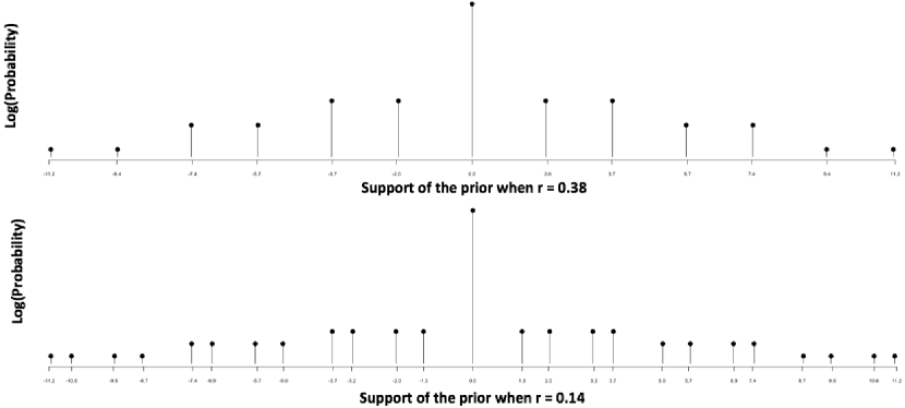
Figure 1. Schematic for our proposed univariate cluster prior when $r$ equals 0.38 (top) and 0.14 (bottom) respectively. The x-axis shows the spacings between and within the clusters and the y-axis the logarithm of the prior probabilities. Figure drawn to scale with $\eta=0.001$. Only the six clusters are displayed with the rest being truncated.

Now, consider the multivariate clustered prior $\pi^{\sf C}_{n}[\eta_{n},r](d\theta)=\prod_{i=1}^{n}\pi_{\sf C}[\eta_{n},r](d\theta_{i})$ on $\mathbb{R}^{n}$. Then, the Bayes prde $\hat{p}_{\sf C}[\eta_{n},r]$ based on $\pi^{\sf C}_{n}[\eta,n]$ is asymptotically minimax optimal.

Theorem 1.1.

Fix any $r\in(0,\infty)$. If $\eta_{n}=s_{n}/n\to 0$, then

$$\lim_{n\to\infty}\;\bigg{\{}\sup_{\theta\in\Theta_{0}[s_{n}]}\rho\big{(}\theta,\hat{p}_{\sf C}[\eta_{n},r]\big{)}\bigg{\}}\bigg{/}R^{*}(\Theta_{0}[s_{n}])=1.$$

Background. For understanding the decision theoretic implications of the above result, we briefly revisit the risk properties of sparse product priors based on symmetric marginals. It follows from J94 that for point estimation of the normal mean over $\Theta_{0}[s_{n}]$ under $\ell_{2}$ loss, the posterior mean of the grid prior $\pi_{n}^{\sf EG}$ is minimax optimal as $\eta_{n}\to 0$. $\pi_{n}^{\sf EG}$ constitutes of i.i.d. copies of univariate grid prior $\pi_{\sf EG}[\eta_{n},r]$ which is defined for any fixed $r$ and $\eta\in(0,1)$ as

$$\pi_{\sf EG}[\eta,r]=(1-\eta)\delta_{0}+\frac{1-\eta}{2}\sum_{i=1}^{\infty}\eta^{i}\big{\{}\delta_{i\lambda_{e}}+\delta_{-i\lambda_{e}}\big{\}}~{}.$$

In contrast to $\pi_{\sf C}$, $\pi_{\sf EG}$ always has only one point in each cluster. However, they have identical probability decay rate as the clusters extend away from the origin. MJ17 showed that the prde based on $\pi_{n}^{\sf EG}$ is sub-optimal for prde estimation based on KL loss. The Bayes prde based on a product grid prior whose univariate marginals $\pi_{\sf PG}$ (subscripts PG and EG denote predictive and estimative grids) has reduced spacing between the atoms and reduced probability decay rate, was established to be minimax optimal in the predictive regime abet for $r\geq\tilde{r}_{0}=(\sqrt{5}-1)/4$:

$$\pi_{\sf PG}[\eta,r]=(1-\eta)\delta_{0}+\frac{\eta(1-\eta^{v})}{2}\sum_{i=1}^{\infty}\eta^{(i-1)v}\big{\{}\delta_{i\lambda_{f}}+\delta_{-i\lambda_{f}}\big{\}}~{}.$$

For constructing a minimax optimal Bayes prde for all values of $r$, MJ17 suggested using a bi-grid prior with two different sections: inner and outer. While the outer section has the spacing and decay rate of $\pi_{\sf PG}$ the inner section has further reduced spacing. Let $b:=b(r)=\min\{4r(1+r)/(1+2r),1\}$ and $J=1+\lceil 2b^{-3/2}\rceil$. For any integer $j$ and $l$, define the inner section support points ${\sf I}_{j}=\text{sign}(j)\{\lambda_{f}+b(|j|-1)\lambda_{f}\}$ and the outer section atoms ${\sf O}_{l}=\text{sign}(l)\{I_{J}+|l|\lambda_{f}\}$. Then, the univariate bi-grid prior is:

$$\pi_{\sf BG}[\eta,r]=(1-\eta)\delta_{0}+\frac{\eta\,c(\eta,r)}{2}\bigg{[}\sum_{j=1}^{J}\eta^{(j-1)b^{2}v}\big{\{}\delta_{{\sf I}_{j}}+\delta_{{\sf I}_{-j}}\big{\}}+\eta^{(J-1)b^{2}v}\sum_{l=1}^{\infty}\eta^{lv}\big{\{}\delta_{{\sf O}_{l}}+\delta_{{\sf O}_{-l}}\big{\}}\bigg{]}$$

where, $c(\eta,r)$ is the normalizing constant defined in eqn. (28) of MJ17. The multivariate prior $\prod_{i=1}^{n}\pi_{\sf BG}[\eta_{n},r](d\theta_{i})$ is minimax optimal for any $r$. Note that $\pi_{\sf BG}$ agrees with $\pi_{\sf PG}$ for $r\geq\tilde{r}_{0}$.

Discussion. Unlike the univariate grid priors $\pi_{\sf EG},\pi_{\sf PG}$ where support points has geometric probability decay, $\pi_{\sf C}$ has support points with identical probability within each clusters. The clusters in $\pi_{\sf C}$ however has the same decay rate as the support points in $\pi_{\sf EG}$. The maximum gap between atoms in $\pi_{\sf C}$ equals the spacing in $\pi_{\sf PG}$. Equiprobable atoms in the clusters was introduced in MJ15 to control predictive risk via the new notion of risk diversification. As such consider a truncated cluster prior with only two clusters: $\pi_{\sf TC}[\eta,r]=(1-\eta)\delta_{0}+{\eta}/{2}\{C_{1}+C_{-1}\}$ where $C_{1}=C_{1}(\eta,r;\tilde{\gamma}_{r},\tilde{K}_{r})$ as in (1.3) with $\tilde{\gamma}_{r}=1+2r$ and $\tilde{K}_{r}$ given by $K_{r}-1$ with the formula in (1.4) used with $\tilde{\gamma}_{r}$ in place of $\gamma_{r}$. As the prior $\pi_{\sf TC}$ is bounded at $\lambda_{e}$, its corresponding Bayes prde $\hat{p}_{\sf CT}$ has unbounded risk. Thresholded product prde $\hat{p}^{\sf T}_{n}(y|x)=\prod_{i=1}^{n}\hat{p}_{\sf T}(y_{i}|x_{i})$ with

$$\hat{p}_{\sf T}(y_{i}|x_{i})=\hat{p}_{\sf TC}[\eta_{n},r](y_{i}|x_{i})1\{|x_{i}|\leq\lambda_{e}(\eta_{n})\}+\phi(y_{i}|x_{i},v_{x}+v_{y})1\{|x_{i}|>\lambda_{e}(\eta_{n})\}~{}$$

was shown in MJ15 to be minimax optimal. Note that, the thresholding was done at the boundary $\lambda_{e}(\eta_{n})$ of the truncated univariate prior; above the threshold the Bayes prde based on the uniform prior, which is Gaussian with variance $v_{x}+v_{y}$, was used. Thresholding rules are not smooth functions of the data and it was conjectured in Sec. 6 of MJ15 that periodic clustered priors of the form of (1.2)-(1.3) can attain minimax optimality without the discontinuous thresholding operation. Here, we study the risk properties of such cluster priors and establish minimax optimality of the properly calibrated prior $\pi_{C}$. We found that the common ratio $\tilde{\gamma}_{r}$ used in MJ15 was not optimal and can be increased to $\gamma_{r}$. However, as a consequence of removing thresholding we needed one more atom than MJ15 in our proposed cluster prior $\pi_{\sf C}$ for small values of $r$.

The new phenomenon of risk diversification introduced in MJ15 to obtain minimax optimality of prdes was further extended in MJ17 where it was shown that to attain minimax optimality of Bayes prdes based on discrete priors, the atoms need to be much denser near the origin that away from the origin. The inner section spacing $b(r)$ of the bi-grid prior $\pi_{\sf BG}$ of MJ17 is slightly lower but quite close to the minimal within cluster spacing in $\pi_{\sf C}$. An intrinsic difference between $\pi_{\sf C}$ and $\pi_{\sf BG}$ is that for $\eta\to 0$ the first cluster $C_{1}$ protrudes much beyond inner section of $\pi_{\sf BG}$, particularly for smaller values of $r$. Though the Bayes prdes from the cluster prior and the bi-grid prior are both minimax optimal (compare theorem 1 here with theorem 1.2 of MJ17), there exists interesting disparity in geometry of their manifolds; subsequently, their maximal risk for them are controlled by different facets of the risk diversification principle. This necessitates separate analysis and proofs of the risk properties of $\pi_{\sf C}$ than that of bi-grid priors.

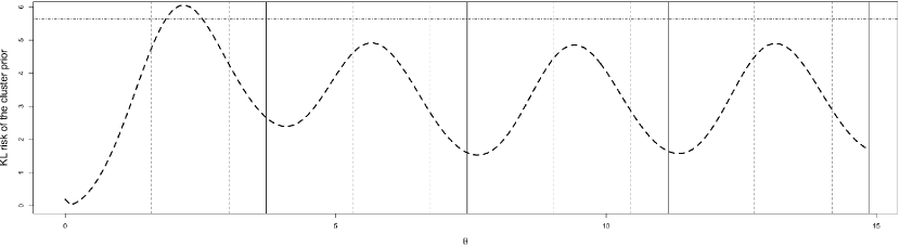
Figure 2. Plot of the univariate predictive KL risk $\rho(\theta,\hat{p}_{\sf C}[\eta,r]$ as $\theta$ varies over the $x$-axis. Here, $\eta=0.001$ and $r=0.225$. The horizontal line corresponds to the asymptotic minimax limit $\lambda^{2}_{f}(\eta)/(2r)$. The dotted vertical lines denotes the location of the non-origin support points of $\pi_{\sf C}[\eta,r]$ with the bold lines marking each cluster boundary.

Figure 2 shows the numerical evaluation of the predictive risk $\rho(\theta,\hat{p}_{\sf C}[\eta,r])$ of the cluster prior based Bayes prde when $\eta=0.001$ and $r=0.225$. Each cluster has size three. The maximum risk $\hat{p}_{\sf C}[\eta,r]$ crosses the asymptotic theory limit but does not exceed by much. It shows that the asymptotic analysis is fairly reflective in this non-asymptotic regime. The risk function has its peak between $\mu_{11}$ and $\mu_{12}$ and is approximately periodic barring a few clusters near the origin. As the figure shows, the risk function is much smaller than the asymptotic limit of $\lambda_{f}^{2}/(2r)$ for all the points in $C_{1}$ barring its first point. As all points in $C_{1}$ are equally likely, this implies that the cluster prior is not least favorable. The following result make this observation rigorous by explicitly evaluating the first order asymptotic Bayes risk of the cluster prior. It establishes that when there are two or more points in each cluster (i.e. $r<r_{0}$) the cluster prior is no longer least favorable. Its Bayes risk, however, has the same order of the minimax risk and will be at least 34% of the minimax risk for any value of $r$.

Theorem 1.2.

If $\eta_{n}=s_{n}/n\to 0$ as $n\to\infty$, then the multivariate cluster prior $\pi^{\sf C}_{n}[\eta_{n},r]$ is not asymptotically least favorable for all $r<r_{0}$. As such, its Bayes risk satisfies:

$$\lim_{n\to\infty}\;\bigg{\{}B(\pi_{n}^{\sf C}[\eta_{n},r])\big{)}\bigg{\}}\bigg{/}R^{*}(\Theta_{0}[s_{n}])=\frac{1}{K_{r}}\bigg{\{}1+r\sum_{i=1}^{\infty}\big{(}1+r^{-1}-(1+4r)^{2i}\big{)}_{+}\bigg{\}}~{},$$

where, $K_{r}$ is defined in (1.4). Additionally, if $\eta_{n}\to 0$ and $s_{n}\to\infty$ as $n\to\infty$ then $\pi^{\sf C}_{n}[\eta_{n},r]$ is asymptotically least favorable for all $r\geq r_{0}$.

2. Proof Layout

We provide a brief overview of the proof of our main result. Detailed proofs are provided in the supplement. The proof of Theorem 1 involves asymptotically upper bounding the risk $\sup_{\theta\in\Theta_{0}[s_{n}]}\rho(\theta,\hat{p}_{\sf C})$ by $R^{*}(\Theta_{0}[s_{n}])$. Then, the asymptotic equality follows as the first term can not be smaller than the minimax risk by definition. Also, note that due to the product structure of the prior, the multivariate maximal risk can be evaluated based on the risk of the univariate Bayes prde $\hat{p}_{\sf C}[\eta_{n},r]$ by using the following relation:

$$\sup_{\theta\in\Theta_{0}[s_{n}]}\rho(\theta,\hat{p}_{\sf C})=n(1-\eta_{n})\rho(0,\hat{p}_{\sf C}[\eta_{n},r])+n\eta_{n}\sup_{\theta\in\mathbb{R}\setminus 0}\rho(\theta,\hat{p}_{\sf C}[\eta_{n},r])~{}.$$ (2.1)

Asymptotic evaluation of the two expressions on the right above is done by using the risk decomposition lemma 2.1 of MJ17. It reduces the calculation for the univariate predictive risk to finding expectation of functionals involving standard normal random variable $Z$ as

$$\rho(\theta,\hat{p}_{\sf C}[\eta_{n},r])=\frac{\theta^{2}}{2r}-\operatorname{\mathbb{E}}\log N_{\theta,v}(Z)+\operatorname{\mathbb{E}}\log D_{\theta}(Z),\text{ where,}$$ (2.2)

$$N_{\theta,v}(Z)=1+\sum_{i\in\mathbb{Z}\setminus 0}\frac{q_{i}}{K}\sum_{j=1}^{K}N_{ij}(\theta,Z;v)\text{ and }D_{\theta}(Z)=N_{\theta,1}(Z)~{}.$$

Here, $q_{i}=(1-\eta_{n})^{-1}P(C_{i})$ with $P(C_{i})$ being the mass of cluster $C_{i}$ in $\pi_{\sf C}[\eta_{n},r]$; thus $q_{i}=2^{-1}\exp(-|i|\lambda_{e,n}^{2}/2)$ with $\lambda_{e,n}=(2\log\eta_{n}^{-1})^{-1}$ and $\lambda_{f,n}=v^{1/2}\lambda_{e,n}$; $N_{ij}$ is the contribution to the risk of the $j$th support point $\mu_{ij}(\eta_{n},r)$ within the $i$th cluster.

The risk contributions $N_{ij}$ are exponents of quadratic forms in $\mu_{ij}$, viz, $N_{ij}(\theta,Z;v)=\exp\{v^{-1/2}{\mu_{ij}Z}+v^{-1}\mu_{ij}\theta-(2v)^{-1}{\mu_{ij}^{2}}\}$. The risk at the origin is well-controlled for this cluster prior based prde (lemma 1 of supplement) and so, based on (2.1), it is suffices to bound $\sup_{\theta}\rho(\theta,\hat{p}_{\sf C}[\eta_{n},r])$ by $\lambda_{f,n}^{2}/(2r)$ to arrive at the desired result. This involves tracing two fundamentally different risk phenomena depending on the location of $\theta$ (a) $\theta\in C_{\pm 1}$ (b) $\theta\notin C_{\pm 1}$. In the former case, $\operatorname{\mathbb{E}}\log D_{\theta}(Z)=O(\lambda_{f,n})$ (by lemma 3 of the supplement) and thus the contribution of the third term on the right of (2.2) is not significant. Also, $\operatorname{\mathbb{E}}\log N_{\theta,v}(Z)=O(\lambda_{f,n})$ for $|\theta|\leq\lambda_{f,n}$ and so, asymptotically $\rho(\theta,\hat{p}_{\sf C}[\eta_{n},r])$ initially increases quadratically in $\theta$ and $\rho(\lambda_{f,n},\hat{p}_{\sf C}[\eta_{n},r])=\lambda_{f,n}^{2}/(2r)(1+o(1))$. However, if $|\theta|\in C_{1}\setminus[0,\lambda_{f,n}]$, then $\operatorname{\mathbb{E}}\log N_{\theta,v}(Z)$ is significantly large and controls the predictive risk below the desired asymptotic limit (see lemma 4 of supplement).

If $\theta\in C_{i}$ for any $|i|>1$, then the risk phenomenon is quite different than the origin adjoining clusters. Now, $\operatorname{\mathbb{E}}\log D_{\theta}(Z)$ is significantly positive. However, an important ingredient of the proof is that its magnitude can be asymptotically well controlled by considering only atoms in $C_{i}$ or the nearest atom in $C_{i-1}$. Lemma 3 in the supplementary material establishes that for $\theta\in C_{i}$ with $|i|>1$, $\operatorname{\mathbb{E}}\log D_{\theta}(Z)\leq\{\operatorname{\mathbb{E}}\log D_{i.}(Z)\}_{+}+o(\lambda^{2}_{f,n})\text{ where }D_{i.}(Z)=N_{i-1,K}(\theta,Z;1)+\sum_{j=1}^{K}N_{ij}(\theta,Z;1).$ Next, use the naive bound $\operatorname{\mathbb{E}}\log N_{\theta,v}(Z)\geq\operatorname{\mathbb{E}}\log N_{i.}(Z))$ where $N_{i.}=N_{i-1,K}(\theta,Z;v)+\sum_{j=1}^{K}N_{ij}(\theta,Z;v)$. Now, plugging these two bounds in (2.2) we get the desired upper bound (see lemma 4 of the supplement).

3. Simulations

Table 2. Numerical evaluation of the maximum risk for the different univariate predictive density estimates as the degree of sparsity ($\eta$) and predictive difficulty $r$ varies. The asymptotic minimax risk is reported in ‘A-Theory’ and the subsequent columns report the maximum risk of the estimators as quotients of ‘A-Theory’ values.

Sparsity	r	A-Theory	Plugin	Thresh	E-Grid	P-Grid	Bi-Grid	SUS	Clustered
	1	2.3026	1.0841	0.7057	0.6236	0.7366	0.7366	0.9090	0.7629
	0.5	3.0701	1.6023	0.8822	0.8031	0.8832	0.8832	1.0135	1.2036
0.01	0.25	3.6841	2.6310	0.9235	1.2718	1.0398	1.0079	1.1383	1.0932
	0.1	4.1865	5.6949	1.1074	2.6198	1.2304	1.2239	1.2677	1.3507
	1	5.7565	1.1371	0.7332	0.7407	0.7277	0.7277	0.8665	0.7287
	0.5	7.6753	1.6960	0.8522	0.9543	0.8486	0.8486	0.9599	1.0874
0.00001	0.25	9.2103	2.8120	0.9125	1.4146	0.9781	0.9464	1.0328	1.0376
	0.1	10.4663	6.1542	1.0395	2.7946	1.1049	1.0710	1.1182	1.0932
	1	11.5129	1.2390	0.7958	0.8357	0.7891	0.7891	0.8765	0.7910
1.00E-10	0.5	15.3506	1.8540	0.8810	1.0488	0.8734	0.8734	0.9337	1.1080
	0.25	18.4207	3.0835	0.9451	1.5092	0.9855	0.9629	0.9945	1.0128
	0.1	20.9326	6.7701	1.0191	2.8958	1.1008	1.0138	1.0611	1.0233

We introspect the performance of the aforementioned prdes across different sparsity regimes. The product structure of our estimation framework allows us to concentrate on the maximal risk of the corresponding univariate prdes. In table 2, we report the maximum risk of our proposed clustered prior based Bayes (CB) prde (in last column) as the degree of sparsity $\eta$ and predictive difficulty $r$ varies. The performance of the six following competing methods (a) hard thresholding based plugin estimator (b) thresholding based risk diversified prdre of MJ15 and Bayes prdes based on (c) $\pi_{\sf EG}$ prior of J94 (d) $\pi_{\sf PG}$ prior of MJ17 (e) $\pi_{\sf BG}$ prior of MJ17 (f) spike and uniform slab (SUS) prior, are respectively reported in columns 4 to 9 in table 2. Across all regimes the maximum risk of CB-prde is reasonably close to the order of the minimax risk prescribed by the asymptotic theory; for large $r$ values the maximum risk is actually lower than the asymptotic theory prescribed minimax value whereas it is little higher for lower $r$ values, particularly at moderate sparsity. For lower $r$ values, CB-prde is substantially better than that the plugin or grid prior based prdes. Overall, CB-prde has similar performance to that of the risk diversified prdes of MJ15 and MJ17, both of which are asymptotically minimax optimal for all $r$.

Supplementary Materials and Acknowledgement

Detailed proofs of the results stated in Section 1 are provided in the supplementary materials. GM is indebted to Professor Iain Johnstone for numerous stimulating discussions which led to many of the ideas in this paper. The research here was partially supported by NSF DMS-1811866.

References

- Aitchison [1975] Aitchison, J. (1975). Goodness of prediction fit. Biometrika 62, 547–554.
- Aitchison & Dunsmore [1975] Aitchison, J. & Dunsmore, I. R. (1975). Statistical prediction analysis. Cambridge University Press.
- Bickel [1983] Bickel, P. (1983). Minimax estimation of the mean of a normal distribution subject to doing well at a point. In Recent Advances in Statistics. Elsevier, pp. 511–528.
- Brown et al. [2008] Brown, L. D., George, E. I. & Xu, X. (2008). Admissible predictive density estimation. Ann. Statist. 36, 1156–1170.
- Clyde & George [2000] Clyde, M. & George, E. I. (2000). Flexible empirical bayes estimation for wavelets. Journal of the Royal Statistical Society: Series B (Statistical Methodology) 62, 681–698.
- Fourdrinier et al. [2011] Fourdrinier, D., Marchand, É., Righi, A. & Strawderman, W. E. (2011). On improved predictive density estimation with parametric constraints. Electron. J. Stat. 5, 172–191.
- Geisser [1993] Geisser, S. (1993). Predictive inference, vol. 55 of Monographs on Statistics and Applied Probability. New York: Chapman and Hall. An introduction.
- George et al. [2006] George, E. I., Liang, F. & Xu, X. (2006). Improved minimax predictive densities under Kullback-Leibler loss. Ann. Statist. 34, 78–91.
- George et al. [2012] George, E. I., Liang, F. & Xu, X. (2012). From minimax shrinkage estimation to minimax shrinkage prediction. Statist. Sci. 27, 82–94.
- Ghosh & Kubokawa [2018] Ghosh, M. & Kubokawa, T. (2018). Hierarchical bayes versus empirical bayes density predictors under general divergence loss. Biometrika .
- Ghosh et al. [2008] Ghosh, M., Mergel, V. & Datta, G. S. (2008). Estimation, prediction and the Stein phenomenon under divergence loss. J. Multivariate Anal. 99, 1941–1961.
- Johnstone [1994] Johnstone, I. M. (1994). On minimax estimation of a sparse normal mean vector. Ann. Statist. 22, 271–289.
- Johnstone [2013] Johnstone, I. M. (2013). Gaussian estimation: Sequence and wavelet models Version: 11 June, 2013. Available at "http://www-stat.stanford.edu/~imj".
- Johnstone & Silverman [2004] Johnstone, I. M. & Silverman, B. W. (2004). Needles and straw in haystacks: empirical Bayes estimates of possibly sparse sequences. Ann. Statist. 32, 1594–1649.
- Kempthorne [1987] Kempthorne, P. J. (1987). Numerical specification of discrete least favorable prior distributions. SIAM Journal on Scientific and Statistical Computing 8, 171–184.
- Komaki [2001] Komaki, F. (2001). A shrinkage predictive distribution for multivariate normal observables. Biometrika 88, 859–864.
- Kubokawa et al. [2013] Kubokawa, T., Marchand, É., Strawderman, W. E. & Turcotte, J.-P. (2013). Minimaxity in predictive density estimation with parametric constraints. Journal of Multivariate Analysis 116, 382–397.
- Kullback & Leibler [1951] Kullback, S. & Leibler, R. A. (1951). On information and sufficiency. Ann. Math. Statistics 22, 79–86.
- Liang [2002] Liang, F. (2002). Exact minimax procedures for predictive density estimation and data compression. ProQuest LLC, Ann Arbor, MI. Thesis (Ph.D.)–Yale University.
- Marchand et al. [2004] Marchand, E., Strawderman, W. E. et al. (2004). Estimation in restricted parameter spaces: A review. In A Festschrift for Herman Rubin. Institute of Mathematical Statistics, pp. 21–44.
- Maruyama & Ohnishi [2016] Maruyama, Y. & Ohnishi, T. (2016). Harmonic bayesian prediction under alpha-divergence. arXiv preprint arXiv:1605.05899 .
- Mukherjee [2013] Mukherjee, G. (2013). Sparsity and Shrinkage in Predictive Density Estimation. Ph.D. thesis, Stanford University.
- Mukherjee & Johnstone [2015] Mukherjee, G. & Johnstone, I. M. (2015). Exact minimax estimation of the predictive density in sparse gaussian models. Annals of Statistics .
- Mukherjee & Johnstone [2017] Mukherjee, G. & Johnstone, I. M. (2017). On minimax optimality of sparse bayes predictive density estimates. arXiv preprint arXiv:1707.04380 .
- Rockova & George [2018] Rockova, V. & George, E. I. (2018). The spike-and-slab lasso. Journal of the American Statistical Association 113, 431–444.
- Xu & Liang [2010] Xu, X. & Liang, F. (2010). Asymptotic minimax risk of predictive density estimation for non-parametric regression. Bernoulli 16, 543–560.