FiBiNET: Combining Feature Importance and Bilinear feature Interaction for Click-Through Rate Prediction

Abstract.

Advertising and feed ranking are essential to many Internet companies such as Facebook and Sina Weibo. Among many real-world advertising and feed ranking systems, click through rate (CTR) prediction plays a central role. There are many proposed models in this field such as logistic regression, tree based models, factorization machine based models and deep learning based CTR models. However, many current works calculate the feature interactions in a simple way such as Hadamard product and inner product and they care less about the importance of features. In this paper, a new model named FiBiNET as an abbreviation for Feature Importance and Bilinear feature Interaction NETwork is proposed to dynamically learn the feature importance and fine-grained feature interactions. On the one hand, the FiBiNET can dynamically learn the importance of features via the Squeeze-Excitation network (SENET) mechanism; on the other hand, it is able to effectively learn the feature interactions via bilinear function. We conduct extensive experiments on two real-world datasets and show that our shallow model outperforms other shallow models such as factorization machine(FM) and field-aware factorization machine(FFM). In order to improve performance further, we combine a classical deep neural network(DNN) component with the shallow model to be a deep model. The deep FiBiNET consistently outperforms the other state-of-the-art deep models such as DeepFM and extreme deep factorization machine(XdeepFM).

1. Introduction

Advertising and feed ranking are essential to many Internet companies such as Facebook and Sina Weibo. The main technique behind these tasks is click-through rate prediction which is known as CTR. Many models have been proposed in this field such as logistic regression (LR)(McMahan et al., 2013), polynomial-2 (Poly2)(Juan et al., 2016), tree based models(He et al., 2014), tensor-based models(Koren et al., 2009), Bayesian models(Graepel et al., 2010), and factorization machines based models(Rendle, 2010, 2012; Juan et al., 2016, 2017).

With the great success of deep learning in many research fields such as computer vision(Krizhevsky et al., 2012; He et al., 2016) and natural language processing(Mikolov et al., 2010; Cho et al., 2014), many deep learning based CTR models have been proposed in recent years(Zhang et al., 2016; Cheng et al., 2016; Xiao et al., 2017; Guo et al., 2017; Lian et al., 2018; Wang et al., 2017; Zhou et al., 2018; He and Chua, 2017). As a result, the deep learning for CTR prediction has also been a research trend in this field. Some neural network based models have been proposed and achieved success such as Factorization-Machine Supported Neural Networks (FNN)(Zhang et al., 2016), Wide&Deep model(WDL)(Cheng et al., 2016), Attentional Factorization Machines(AFM)(Xiao et al., 2017), DeepFM(Guo et al., 2017), XDeepFM(Lian et al., 2018) etc.

In this paper, a new model named FiBiNET as an abbreviation for Feature Importance and Bilinear feature Interaction NETwork is proposed to dynamically learn the feature importance and fine-grained feature interactions. As far as we know, different features have various importances for the target task. For example, the feature occupation is more important than the feature hobby when we predict a person’s income. Taking this into consideration, we introduce a Squeeze-and-Excitation network (SENET)(Hu et al., 2017) to learn the weights of features dynamically. Besides, feature interaction is a key challenge in CTR prediction field and many related works calculate the feature interactions in a simple way such as Hadamard product and inner product. We propose a new fine-grained way in this paper to calculate the feature interactions with the bilinear function. Our main contributions are listed as follows:

• Inspired by the success of SENET in the computer vision field, we use the SENET mechanism to learn the weights of features dynamically.

• We introduce three types of Bilinear-Interaction layer to learn feature interactions in a fine-grained way. This is also in contrast to the previous work(Juan et al., 2016, 2017; Xiao et al., 2017; Rendle, 2010, 2012; He and Chua, 2017), which calculates the feature interactions with Hadamard product or inner product.

• Combining SENET mechanism with bilinear feature interaction, our shallow model achieves state-of-the-art among the shallow models such as FFM on Criteo and Avazu datasets.

• For further performance gains, we combine a classical deep neural network(DNN) component with the shallow model to be a deep model. The deep FiBiNET consistently outperforms the other state-of-the-art deep models on Criteo and Avazu datasets.

The rest of this paper is organized as follows. In Section 2, we review related works which are relevant with our proposed model, followed by introducing our proposed model in Section 3. We will present experimental explorations on Criteo and Avazu datasets in Section 4. Finally, we discuss empirical results and conclude this work in Section 5.

2. Related Work

2.1. Factorization Machine and Its relevant variants

Factorization machine(FM)(Rendle, 2010, 2012) and field-aware factorization machine (FFM)(Juan et al., 2016, 2017) are two of the most successful CTR models. FM models all feature interactions between variables using factorized parameters. It has a low time complexity and memory storage, and it works well on large sparse data. FFM introduced field aware latent vectors and won two competitions hosted by Criteo and Avazu(Juan et al., 2017). However, FFM was restricted by the need of large memory and cannot easily be used in Internet companies.

2.2. Deep Learning based CTR Models

Deep learning has achieved great success in many research fields such as computer vision(Krizhevsky et al., 2012; He et al., 2016) and natural language processing(Mikolov et al., 2010; Cho et al., 2014). As a result, many deep learning based CTR models have also been proposed in recent years(Zhang et al., 2016; Cheng et al., 2016; Xiao et al., 2017; Guo et al., 2017; Lian et al., 2018; Wang et al., 2017; Zhou et al., 2018; He and Chua, 2017). How to effectively model the feature interactions is the key factor for most of these neural network based models.

Factorization-Machine Supported Neural Networks (FNN)(Zhang et al., 2016) is a forward neural network using FM to pre-train the embedding layer. However, FNN can capture only high-order feature interactions. Wide & Deep model(WDL)(Cheng et al., 2016) was initially introduced for application recommendation in google play. WDL jointly trains wide linear models and deep neural networks to combine the benefits of memorization and generalization for recommender systems. However, expertise feature engineering is still needed on the input to the wide part of WDL, which means that the cross-product transformation also requires to be manually designed. To alleviate manual efforts in feature engineering, DeepFM(Guo et al., 2017) replaces the wide part of WDL with FM and shares the feature embedding between the FM and deep component. DeepFM is regarded as one state-of-the-art model in CTR estimation field.

Deep & Cross Network (DCN)(Wang et al., 2017) efficiently captures feature interactions of bounded degrees in an explicit fashion. Similarly, eXtreme Deep Factorization Machine (xDeepFM)(Lian et al., 2018) also models the low-order and high-order feature interactions in an explicit way by proposing a novel Compressed Interaction Network (CIN) part.

As (Xiao et al., 2017) mentioned, FM can be hindered by its modeling of all feature interactions with the same weight, as not all feature interactions are equally useful and predictive. And they propose the Attentional Factorization Machines(AFM)(Xiao et al., 2017) model, which uses an attention network to learn the weights of feature interactions. Deep Interest Network (DIN)(Zhou et al., 2018) represents users’ diverse interests with an interest distribution and designs an attention-like network structure to locally activate the related interests according to the candidate ad.

2.3. SENET Module

Hu (Hu et al., 2017) proposed the “Squeeze-and-Excitation Network” (SENET) to improve the representational power of a network by explicitly modeling the interdependencies between the channels of convolutional features in various image classification tasks. The SENET is proved to be successful in image classification tasks and won first place in the ILSVRC 2017 classification task.

There are also other applications about SENET except for the image classification(Yan et al., 2018; Kitada and Iyatomi, 2018; Roy et al., 2018). (Roy et al., 2018) introduces three variants of the SE modules for semantic segmentation task. Classifying common thoracic diseases as well as localizing suspicious lesion regions on chest X-rays(Yan et al., 2018) is another application field. (Linsley et al., 2018) extends SENET module with a global-and-local attention (GALA) module to get state-of-the-art accuracy on ILSVRC.

3. Our Proposed Model

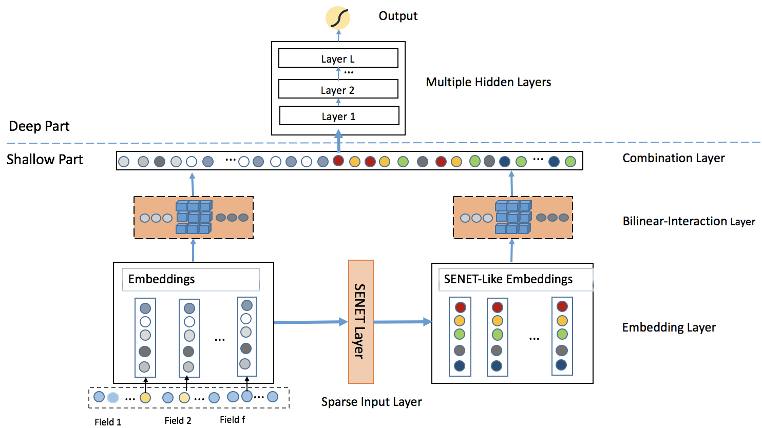
Figure 1. The architecture of our proposed FiBiNET

We aim to dynamically learn the importance of features and feature interactions in a fine-grained way. To this end, we propose the Feature Importance and Bilinear feature Interaction NETwork(FiBiNET) for CTR prediction tasks.

In this section, we will describe the architecture of our proposed model as depicted in Figure 1. For clarity purpose, we omit the logistic regression part which can be trivially incorporated. Our proposed model consists of the following parts: sparse input layer, embedding layer, SENET layer, Bilinear-Interaction layer, combination layer, multiple hidden layers and output layer. The sparse input layer and embedding layer are the same with DeepFM(Guo et al., 2017), which adopts a sparse representation for input features and embeds the raw feature input into a dense vector. The SENET layer can convert an embedding layer into the SENET-Like embedding features, which helps to boost feature discriminability. The following Bilinear-Interaction layer models second order feature interactions on the original embedding and the SENET-Like embedding respectively. Subsequently, these cross features are concatenated by a combination layer which merges the outputs of Bilinear-Interaction layer. At last, we feed the cross features into a deep neural network and the network outputs the prediction score.

3.1. Sparse Input and Embedding layer

The sparse input layer and embedding layer are widely used in deep learning based CTR models such as DeepFM(Guo et al., 2017) and AFM(Xiao et al., 2017). The sparse input layer adopts a sparse representation for raw input features. The embedding layer is able to embed the sparse feature into a low dimensional, dense real-value vector. The output of embedding layer is a wide concatenated field embedding vector: $E=[e_{1},e_{2},\cdots,e_{i},\cdots,e_{f}]$, where $f$ denotes the number of fields, $e_{i}\in R^{k}$ denotes the embedding of $i$-th field , and $k$ is the dimension of embedding layer.

3.2. SENET Layer

As far as we know, different features have various importances for the target task. For example, the feature occupation is more important than the feature hobby when we predict a person’s income. Inspired by the success of SENET in the computer vision field, we introduce a SENET mechanism to let the model pay more attention to the feature importance. For specific CTR prediction task, we can dynamically increase the weights of important features and decrease the weights of uninformative features via the SENET mechanism.

Using the feature embedding as input, the SENET produces weight vector $A=\{a_{1},\cdots,a_{i},\cdots,a_{f}\}$ for field embeddings and then rescales the original embedding $E$ with vector $A$ to get a new embedding (SENET-Like embedding) $V=[v_{1},\cdots,v_{i},\cdots,v_{f}]$, where $a_{i}\in R$ is a scalar that denotes the weight of the $i$-th field embedding $v_{i}$, $v_{i}\in R^{k}$ denotes the SENET-Like embedding of $i$-th field, $i\in[1,2,\cdots,f]$ , $V$ $\in$ $R^{f\times k}$ , $k$ is an embedding size, and $f$ is the number of fields.

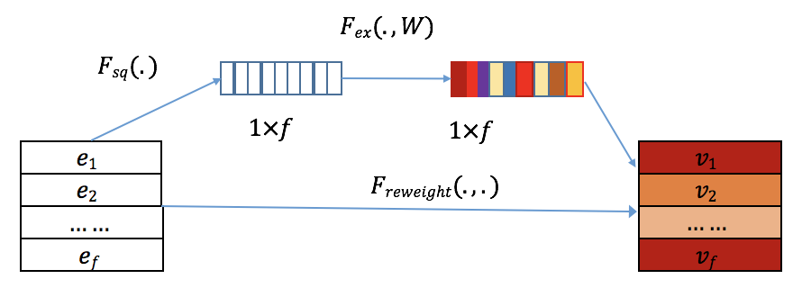
Figure 2. The SENET Layer

As Figure 2 illustrated, the SENET is comprised of three steps: squeeze step, excitation step and re-weight step. These steps can be described in detail as follows:

Squeeze. This step is used for calculating ’summary statistics’ of each field embedding. Concretely speaking, we use some pooling methods such as max or mean to squeeze the original embedding $E=[e_{1},\cdots,e_{f}]$ into a statistic vector $Z=[z_{1},\cdots,z_{i},\cdots,z_{f}]$, where $i\in[1,\cdots,f]$, $z_{i}$ is a scalar value which represents the global information about the $i$-th feature representation. $z_{i}$ can be calculated as the following global mean pooling:

(1) $$z_{i}=F_{sq}(e_{i})=\frac{1}{k}{\sum_{t=1}^{k}e_{i}^{(t)}}$$

The squeeze function in original SENET paper(Hu et al., 2017) is max pooling. However, our experimental results show that the mean pooling performs better than the max pooling.

Excitation. This step can be used to learn the weight of each field embedding based on the statistic vector $Z$. We use two full connected (FC) layers to learn the weights. The first FC layer is a dimensionality-reduction layer with parameters $W_{1}$ with reduction ratio $r$ which is a hyper-parameter and it uses $\sigma_{1}$ as nonlinear function. The second FC layer increases dimensionality with parameters $W_{2}$. Formally, the weight of field embedding can be calculated as follows:

(2) $$A=F_{ex}(Z)=\sigma_{2}(W_{2}\sigma_{1}(W_{1}Z))$$

where $A\in R^{f}$ is a vector, $\sigma_{1}$ and $\sigma_{2}$ are activation functions, the learning parameters are $W_{1}\in R^{f\times\frac{f}{r}}$, $W_{2}\in R^{\frac{f}{r}\times f}$, and $r$ is reduction ratio.

Re-Weight. The last step in SENET is a reweight step which is called re-scale in original paper(Hu et al., 2017). It does field-wise multiplication between the original field embedding $E$ and field weight vector $A$ and outputs the new embedding(SENET-Like embedding) $V=\{v_{1},\cdots,v_{i},\cdots,v_{f}\}$. The SENET-Like embedding $V$ can be calculated as follows:

(3) $$V=F_{ReWeight}(A,E)=[a_{1}\cdot e_{1},\cdots,a_{f}\cdot e_{f}]=[v_{1},\cdots,v_{f}]$$

where $a_{i}\in R$, $e_{i}\in R^{k}$, and $v_{i}\in R^{k}$ .

In short, the SENET uses two FCs to dynamically learn the importance of features. For a specific task, it increases the weights of important features and decreases the weights of uninformative features.

3.3. Bilinear-Interaction Layer

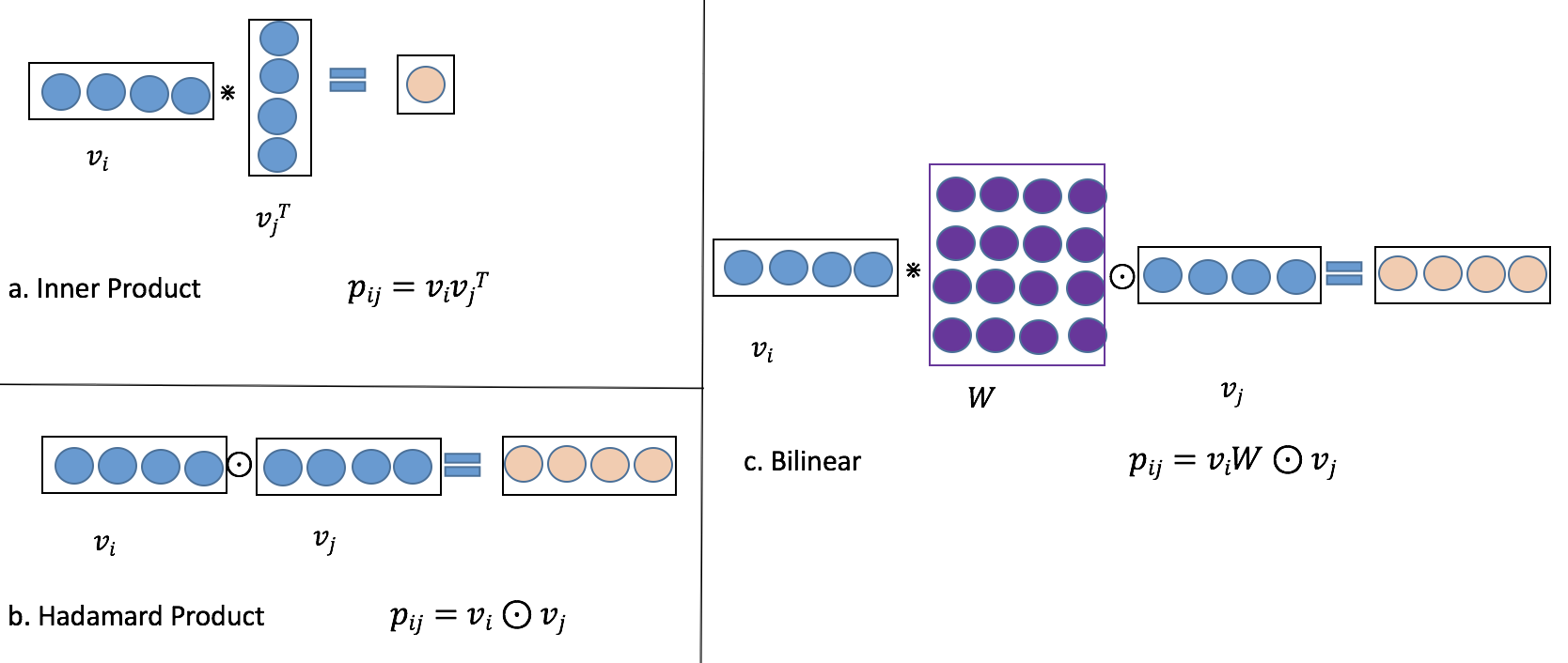
Figure 3. The different methods to calculate the feature interactions. (a): Inner product. (b): Hadamard product. (c): our proposed bilinear interaction. Here $p_{ij}$ in inner product method is a scalar while it is a vector in Hadamard product and our proposed bilinear function.

The Interaction layer is a layer to calculate the second order feature interactions. The classical methods of feature interactions in Interaction layer are inner product and Hadamard product. Inner product is widely used in shallow models such as FM and FFM while the Hadamard product is commonly used in deep models such as AFM and NFM. The forms of inner product and Hadamard product are respectively expressed as $\{(v_{i}\cdot v_{j})x_{i}x_{j}\}_{(i,j)\in R_{x}}$ and $\{(v_{i}\odot v_{j})x_{i}x_{j}\}_{(i,j)\in R_{x}}$ , where $R_{x}=\{(i,j)\}_{i\in\{1,\cdots,f\},j\in\{1,\cdots,f\},j>i}$, $v_{i}$ is the i-th field embedding vector, $\cdot$ denotes the regular inner product, and $\odot$ denotes the Hadamard product, for example, $[a_{1},a_{2},a_{3}]\odot[b_{1},b_{2},b_{3}]=[a_{1}b_{1},a_{2}b_{2},a_{3}b_{3}]$. Inner product and Hadamard product in Interaction layer are too simple to effectively model the feature interactions in sparse dataset. Therefore, we propose a more fine-grained method which combines the inner product and Hadamard product to learn the feature interactions with extra parameters. As shown in Figure 3.c, the inner product is used between the matrix $W$ and vector $v_{i}$ and the Hadamard product is used between the matrix $W$ and the vector $v_{j}$. Specifically, we propose three types of bilinear functions in this layer and call this layer Bilinear-Interaction layer. Taking the $i$-th field embedding $v_{i}$ and the $j$-th field embedding $v_{j}$ as an example, the result of feature interaction $p_{ij}$ can be calculated as follows:

a.Field-All Type

(4) $$p_{ij}=v_{i}\cdot W\odot v_{j}$$

where $W\in R^{k\times k}$, and $v_{i},v_{j}\in R^{k}$ are the $i$-th and $j$-th field embedding, $1\leq i\leq f,i\leq j\leq f$. Here $W$ is shared among all $(v_{i},v_{j})$ field interaction pairs and there are $k\times k$ parameters in Bilinear-Interaction layer, so here we call this type ’Field-All’.

b.Field-Each Type

(5) $$p_{ij}=v_{i}\cdot W_{i}\odot v_{j}$$

where $W_{i}\in R^{k\times k}$, $v_{i},v_{j}\in R^{k}$ are the $i$-th and $j$-th field embedding, $1\leq i\leq f,i\leq j\leq f$ . Here $W_{i}$ is the corresponding parameter matrix of the $i$-th field and there are $f\times k\times k$ parameters in Bilinear-Interaction layer because we have $f$ different fields, so here we call this type ’Field-Each’.

c.Field-Interaction Type

(6) $$p_{ij}=v_{i}\cdot W_{ij}\odot v_{j}$$

where $W_{ij}\in R^{k\times k}$ is the corresponding parameter matrix of interaction between field $i$ and field $j$ and $1\leq i\leq f,i\leq j\leq f$. The total number of learning parameters in this layer is $n\times k\times k$, $n$ is the number of field interactions, which is equal to $\frac{f(f-1)}{2}$. Here we call this type ’Field-Interaction’.

As shown in Figure 1, we have two embeddings(original embedding and SENET-like embedding) and we can adopt either the bilinear function or Hadamard product as feature interaction operation to any embeddings. So we have several combinations of feature interaction in this layer. In Section 4.3, we will discuss the performance of different combinations of bilinear function and Hadamard product in detail. In addition, we have three different types of proposed feature interaction methods(Field-All, Field-Each, Field-Interaction) to apply in our model and we will discuss the performance of different field types in Section 4.4.

In this section, the Bilinear-Interaction layer can output an interaction vector $p=[p_{1},...,p_{i},...,p_{n}]$ from the original embedding $E$ and a SENET-Like interaction vector $q=[q_{1},...,q_{i},...,q_{n}]$ from the SENET-Like embedding $V$, where $p_{i},q_{i}\in R^{k}$ are vectors.

3.4. Combination Layer

The combination layer concatenates interaction vector $p$ and $q$ and feeds the concatenated vector into the following layer in FiBiNET which is a standard neural network layer. It can be expressed as the following forms:

(7) $$c=F_{concat}(p,q)=[p_{1},\cdots,p_{n},q_{1},\cdots,q_{n}]=[c_{1},\cdots,c_{2n}]$$

If we sum each element in vector $c$ and then use a sigmoid function to output a prediction value, we have a shallow CTR model. For further performance gains, we combine the shallow component and a classical deep neural network(DNN) which will be described in Section 3.5 into a unified model to form the deep network structure, this unified model is called deep model in our paper.

3.5. Deep Network

The deep network is comprised of several full-connected layers, which implicitly captures high-order features interactions. As shown in Figure 1, the input of deep network is the output of the combination layer. Let $a^{(0)}=[c_{1},c_{2},\cdots,c_{2n}]$ denotes the outputs of the combination layer, where $c_{i}\in R^{k}$ and $n$ is the number of field interactions. Then, $a^{(0)}$ is fed into the deep neural network and the feed forward process is:

(8) $$a^{(l)}=\sigma(W^{(l)}a^{(l-1)}+b^{(l)})$$

where $l$ is the depth and $\sigma$ is the activation function. $W^{(l)}$,$b^{(l)}$,$a^{(l)}$ are the model weight, bias and output of the $l$-th layer. After that, a dense real-value feature vector is generated which is finally fed into the sigmoid function for CTR prediction: $y_{d}=\sigma(W^{|L|+1}a^{|L|}+b^{|L|+1})$, where $|L|$ is the depth of DNN.

3.6. Output Layer

To summarize, we give the overall formulation of our proposed model’ output as:

(9) $$\hat{y}=\sigma(w_{0}+\sum_{i=0}^{m}{w_{i}x_{i}}+y_{d})$$

where $\hat{y}\in(0,1)$ is the predicted value of CTR, $\sigma$ is the sigmoid function, $m$ is the feature size, $x$ is a input and $w_{i}$ is the $i$-th weight of linear part. The parameters of our model are $\theta=\{w_{0},\{w_{i}\}_{i=1}^{m},\{e_{i}\}_{i=1}^{m},\{W_{i}\}_{i=1}^{2},\{W^{(i)}\}_{i=1}^{|L|}\}$. The learning process aims to minimize the following objective function (cross entropy):

(10) $$loss={-}\frac{1}{N}\sum_{i=1}^{N}({y_{i}}log(\hat{y_{i}})+(1-y_{i})*log(1-\hat{y_{i}}))$$

where $y_{i}$ is the ground truth of $i$-th instance, $\hat{y_{i}}$ is the predicted CTR, and $N$ is the total size of samples.

3.6.1. Relationship with FM and FNN

Suppose we remove the SENET layer and Bilinear-Interaction layer, it’s not hard to find that our model will be degraded as the FNN. When we further remove the DNN part, and at the same time use a constant sum, then the shallow FiBiNET is downgraded to the traditional FM model.

4. Experiments

In this section, we conduct extensive experiments to answer the following questions:

(RQ1) How does our model perform as compared to the state-of-the-art methods for CTR prediction?

(RQ2) Can the different combinations of bilinear and Hadamard functions in Bilinear-Interaction layer impact its performance?

(RQ3) Can the different field types(Field-All, Field-Each and Field-Interaction) of Bilinear-Interaction layer impact its performance?

(RQ4) How do the settings of networks influence the performance of our model?

(RQ5) Which is the most important component in FiBiNET?

We will answer these questions after presenting some fundamental experimental settings.

4.1. Experimental Testbeds and Setup

4.1.1. Data Sets

1) Criteo. The Criteo dataset is widely used in many CTR model evaluation. It contains click logs with 45 millions of data instances. There are 26 anonymous categorical fields and 13 continuous feature fields in Criteo dataset. We split the dataset randomly into two parts: 90% is for training, while the rest is for testing. 2) Avazu. The Avazu dataset consists of several days of ad click-through data which is ordered chronologically. It contains click logs with 40 millions of data instances. For each click data, there are 24 fields which indicate elements of a single ad impression. We split it randomly into two parts: 80% is for training, while the rest is for testing.

4.1.2. Evaluation Metrics

In our experiment, we adopt two metrics: AUC(Area Under ROC) and Log loss.

AUC: Area under ROC curve is a widely used metric in evaluating classification problems. Besides, some work validates AUC as a good measurement in CTR prediction(Graepel et al., 2010). AUC is insensitive to the classification threshold and the positive ratio. The upper bound of AUC is 1, and the larger the better.

Log loss: Log loss is widely used metric in binary classification, measuring the distance between two distributions. The lower bound of log loss is 0, indicating the two distributions perfectly match, and a smaller value indicates better performance.

4.1.3. Baseline Methods

To verify the efficiency of combining SENET layer with Bilinear-Interaction layer in shallow model and deep model, we split our experiments into two groups: shallow group and deep group. We also split the baseline models into two parts: shallow baseline models and deep baseline models. The shallow baseline models include LR(logistic regression)(McMahan et al., 2013), FM(Rendle, 2010, 2012), FFM(Juan et al., 2016, 2017), AFM(Xiao et al., 2017), and the deep baseline models include FNN(Zhang et al., 2016), DCN(Wang et al., 2017), DeepFM(Guo et al., 2017), XDeepFM(Lian et al., 2018).

Note that an improvement of 1‰ in AUC is usually regarded as significant for the CTR prediction because it will bring a large increase in a company’s revenue if the company has a very large user base.

4.1.4. Implementation Details

We implement all the models with Tensorflow in our experiments. For the embedding layer, the dimension of embedding layer is set to 10 for Criteo dataset and 50 for Avazu dataset. For the optimization method, we use the Adam(Kingma and Ba, 2014) with a mini-batch size of 1000 for Criteo and 500 for Avazu datasets, and the learning rate is set to 0.0001. For all deep models, the depth of layers is set to 3, all activation functions are RELU, the number of neurons per layer is 400 for Criteo dataset and 2000 for Avazu dataset, and the dropout rate is set to 0.5. For the SENET part, the activation functions in two FCs are RELU function, and the reduction ratio is set to 3. We conduct our experiments with 2 Tesla K40 GPUs.

4.2. Performance Comparison(RQ1)

In this subsection, we summarize the overall performance of shallow models and deep models on Criteo and Avazu test sets in Table 1 and Table 2 respectively.

Table 1. The overall performance of shallow models on Criteo and Avazu datasets. The SE-FM-ALL denotes the shallow model with the Field-All type of Bilinear-Interaction layer.

	Criteo		Avazu
Model	AUC	Logloss	AUC	Logloss
LR	0.7808	0.4681	0.7633	0.3891
FM	0.7923	0.4584	0.7745	0.3832
FFM	0.8001	0.4525	0.7795	0.3810
AFM	0.7965	0.4541	0.7740	0.3839
SE-FM-All	0.8021	0.4495	0.7803	0.3800

Table 1 shows the results of the shallow models on Criteo and Avazu datasets. We find our shallow SE-FM-All model consistently outperforms other models such as FM, FFM, AFM etc. On the one hand, the results indicate that combining the SENET mechanism with the bilinear interaction over sparse features is an effective method for many real world datasets; on the other hand, for the classical shallow models, the state-of-the-art model is FFM which is restricted by the need of large memory and cannot be easily used in Internet companies, our shallow model has fewer parameters but still performs better than FFM. So it can be regarded as an alternative solution for FFM.

Table 2. The overall performance of deep models on Criteo and Avazu datasets. The DeepSE-FM-ALL denotes the deep model with the Field-All type of Bilinear-Interaction layer.

	Criteo		Avazu
Model	AUC	Logloss	AUC	Logloss
FNN	0.8057	0.4464	0.7802	0.3800
DeepFM	0.8085	0.4445	0.7786	0.3810
DCN	0.7978	0.4617	0.7681	0.3940
XDeepFM	0.8091	0.4461	0.7808	0.3818
DeepSE-FM-All	0.8103	0.4423	0.7832	0.3786

For further performance gains, we combine the shallow part and DNN into a deep model. The overall performance of deep models is shown in Table 2 and we have the following observations:

• Combining the shallow part and DNN into a unified model, the shallow model can gain further performance improvement. We can infer from experimental results that the implicit high-order feature interactions help the shallow model to gain more expressive power.

• Among all the compared methods, our proposed deep FiBiNET achieves the best performance. Our deep model outperforms FNN by relatively 0.571% and 0.386% in terms of AUC(0.918% and 0.4% in terms of log loss) and outperforms DeepFM by 0.222% and 0.59% in terms of AUC(0.494% and 0.6% in terms of log loss) on Criteo and Avazu datasets.

• The results indicate that combining the SENET mechanism with Bilinear-Interaction in DNN for prediction is effective. On the one hand, the SENET intrinsically introduces dynamics conditioned on the input, helping to boost feature discriminability; on the other hand, the bilinear function is an effective method to model the feature interaction as compared with other methods such as the inner product or Hadamard product as described in Section 4.3.

For further performance gains, we will discuss the different combinations of Bilinear-Interaction layer in Section 4.3 and the field types of Bilinear-Interaction layer in Section 4.4.

4.3. Combinations of Bilinear-Interaction Layer(RQ2)

In this section, we will discuss the influence of different type of combinations between bilinear function and Hadamard product in Bilinear-Interaction layer. For convenience, we use 0 and 1 to represent which function is used in Bilinear-Interaction layer. The ’1’ denotes that bilinear function is used while 0 means Hadamard product is used. We have two embeddings so two numbers are used. The first number denotes the feature interaction method used on original embedding and the second number denotes the feature interaction method used on SENET-Like embedding. For example, ’10’ denotes that bilinear function is used as feature interaction method on the original embedding while the Hadamard function is used as feature interaction method on the SENET like embedding. Similarly, we conduct the experiments on shallow and deep models and summarize the results in Table 3.

Table 3. The performance of different combinations of bilinear and Hadamard functions in Bilinear-Interaction layer. The field type of Bilinear-Interaction layer is set to Field-Each.

	Criteo		Avazu
Combinations	AUC	Logloss	AUC	Logloss
SE-FM_00	0.7989	0.4525	0.7782	0.3818
SE-FM_01	0.8018	0.4500	0.7797	0.3808
SE-FM_10	0.8029	0.4488	0.7794	0.3807
SE-FM_11	0.8037	0.4479	0.7770	0.3815
DeepSE-FM-00	0.8105	0.4425	0.7828	0.3785
DeepSE-FM-01	0.8104	0.4423	0.7833	0.3783
DeepSE-FM-10	0.8100	0.4427	0.7810	0.3809
DeepSE-FM-11	0.8099	0.4428	0.7805	0.3807

Overall, we can not draw any obvious conclusions, but we can find some empirical observations as follows:

• On Criteo dataset, the combination ’11’ outperforms other type of combinations among shallow models. However, the combination ’11’ performs worst among the deep models.

• The preferred combination in deep models should be ’01’. This combination means the bilinear function is only applied to the SENET-Like embedding layer, which is beneficial for designing an effective network architectures in our model.

4.4. Field Types of Bilinear-Interaction (RQ3)

Table 4. The performance of different field types of Bilinear-Interaction layer.

	Criteo		Avazu
Field Types	AUC	Logloss	AUC	Logloss
SE-FM-All	0.8021	0.4495	0.7804	0.3800
SE-FM-Each	0.8037	0.4479	0.7797	0.3812
SE-FM-Interaction	0.8059	0.4460	0.7785	0.3815
DeepSE-FM-All	0.8103	0.4423	0.7832	0.3786
DeepSE-FM-Each	0.8104	0.4423	0.7833	0.3783
DeepSE-FM-Interaction	0.8105	0.4421	0.7828	0.3788

In this section, we study impact of different field types(Field-All, Field-Each and Field-Interaction) of Bilinear-Interaction layer. We first fix the combination of the bilinear and Hadamard product in Bilinear-Interaction layer. The combination of Bilinear-Interaction layer is set to ’01’ for deep model and ’11’ for shallow model. And the mark ’01’ and ’11’ are illustrated in Section 4.3. We summarize the experimental results in Table 4 and have the following observations:

• For the shallow models, compared to the Field-All type of our shallow model (in Table 1), the Field-Interaction type can gains 0.382% (relatively 0.476%) improvements in terms of AUC on Criteo dataset.

• For the deep models, compared to the Field-All type of our deep model (in Table 2), the type of Field-Interaction for Criteo dataset and Field-Each for Avazu dataset can gain some improvements respectively.

• The performances of different types of Bilinear-Interaction layer depend on datasets. On Criteo dataset, the performance ranking is as follows: Field-Interaction, Field-Each, and Field-All. While on Avazu dataset, we cannot draw the obvious conclusion.

4.5. Hyper-parameter Investigation(RQ4)

In this subsection, we will conduct some hyper-parameter investigations in our model. We focus on hyper-parameters in the following two components in FiBiNET: the embedding part and the DNN part. Specifically, we change the following hyper-parameters:(1) the dimension of embeddings; (3) the number of neurons per layer in DNN; (4) the depth of DNN. Unless specially mentioned in our paper, the default parameter of our network is set as the Section 4.1.4.

4.5.1. Embedding Part

Table 5. The performance of different embedding sizes on Criteo and Avazu datasets

	Criteo		Avazu
Embedding-Size	AUC	Logloss	AUC	Logloss
10	0.8104	0.4423	0.7809	0.3801
20	0.8093	0.4435	0.7810	0.3796
30	0.8071	0.4460	0.7812	0.3799
40	0.8071	0.4464	0.7824	0.3790
50	0.8072	0.4468	0.7833	0.3787

We change the embedding sizes from 10 to 50 and summarize the experimental results in Table 5. We can find some observations as follows:

• As the dimension is expanded from 10 to 50, our model can obtain a substantial improvement on Avazu dataset.

• The performance degrades when we increase the embedding size on Criteo dataset. Enlarging embedding size indicates increasing the number of parameters in embedding layer and DNN part. We guess that it may be the much more features in Criteo dataset as opposed to Avazu dataset that leads to optimization difficulties.

4.5.2. DNN Part

In deep part, we can change the number of neurons per layer, the depths of DNN, the activation functions and the dropout rates. For brevity, we just study the impact of different neural units per layer and different depths in DNN part.

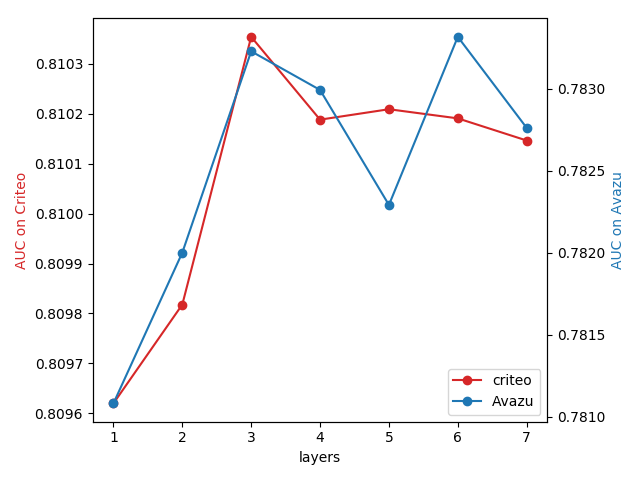
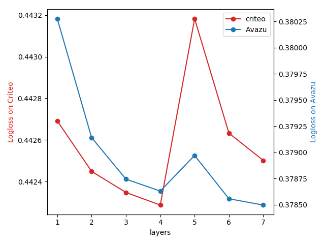
Figure 4. The performance of different number of layers in DNN.

As a matter of fact, increasing the number of layers can increase the model complexity. We can observe from Figure 4 that increasing number of layers improves model performance at the beginning. However, the performance is degraded if the number of layers keeps increasing. This is because an over-complicated model is easy to overfit. It’s a good choice that the number of hidden layers is set to 3 for Avazu dataset and Criteo dataset. Likewise, increasing the number of neurons per layer introduces complexity. In Figure 5, we find that it is better to set 400 neurons per layer for Criteo dataset and 2000 neurons per layer for Avazu dataset.

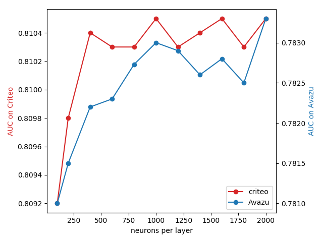
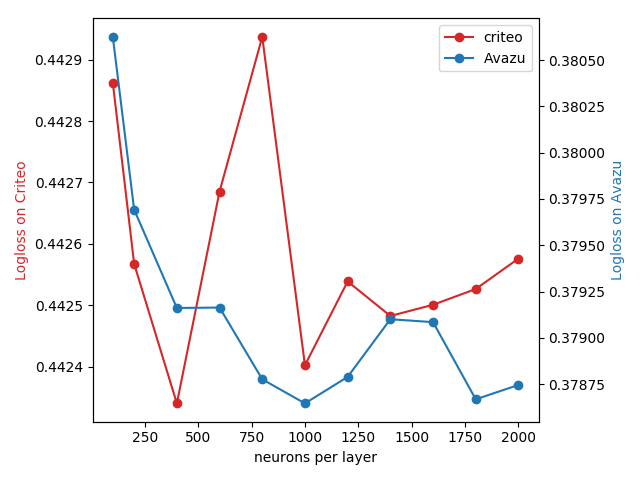
Figure 5. The performance of different number of neurons per layer in DNN

4.6. Ablation Study (RQ5)

Table 6. The performance of different components in FiBiNET.

	Criteo		Avazu
Model	AUC	Logloss	AUC	Logloss
BASE	0.8037	0.4479	0.7797	0.3812
NO-SE	0.7962	0.4552	0.7763	0.3825
NO-BI	0.7986	0.4525	0.7754	0.3829
FM	0.7923	0.4584	0.7745	0.3832
Deep-BASE	0.8104	0.4423	0.7833	0.3783
NO-SE	0.8098	0.4427	0.7822	0.3790
NO-BI	0.8093	0.4435	0.7827	0.3785
FNN	0.8057	0.4464	0.7802	0.3800

Although we have demonstrated strong empirical results, the results presented so far have not isolated the specific contributions from each component of the FiBiNET. In this section, we perform ablation experiments over FiBiNET in order to better understand their relative importance. We set ‘DeepSE-FM-Interaction’ as the base model and perform it in the following ways: 1) No BI: remove the Bilinear-Interaction layer from FiBiNET 2) No SE: remove the SENET layer from FiBiNET.

If we remove the SENET layer and Bilinear-Interaction layer, our shallow FiBiNET and deep FiBiNET will downgrade to FM and FNN. We can find the following observations in Table 6:

• Both the Bilinear-Interaction layer and SENET layer are necessary for FiBiNET’s performance. We can see that the the performance will drop apparently when we remove any component.

• The Bilinear-Interaction layer is as important as the SENET layer in FiBiNET.

5. Conclusions

Motivated by the drawbacks of the state-of-the-art models, we propose a new model named FiBiNET as an abbreviation for Feature Importance and Bilinear feature Interaction NETwork and aim to dynamically learn the feature importance and fine-grained feature interactions. Our proposed FiBiNET makes a contribution to improving performance in these following aspects: 1) For CTR task, the SENET module can learn the importance of features dynamically. It boosts the weight of the important feature and suppresses the weight of unimportant features. 2) We introduce three types of Bilinear-Interaction layers to learn feature interaction rather than calculating the feature interactions with Hadamard product or inner product. 3) Combining the SENET mechanism with bilinear feature interaction in our shallow model outperforms other shallow models such as FM and FFM. 4) In order to improve performance further, we combine a classical deep neural network(DNN) component with the shallow model to be a deep model. The deep FiBiNET consistently outperforms the other state-of-the-art deep models such as DeepFM and XdeepFM.

References

- (1)
- Cheng et al. (2016) Heng-Tze Cheng, Levent Koc, Jeremiah Harmsen, Tal Shaked, Tushar Chandra, Hrishi Aradhye, Glen Anderson, Greg Corrado, Wei Chai, Mustafa Ispir, et al. 2016. Wide & deep learning for recommender systems. In Proceedings of the 1st Workshop on Deep Learning for Recommender Systems. ACM, 7–10.
- Cho et al. (2014) Kyunghyun Cho, Bart van Merrienboer, Caglar Gulcehre, Dzmitry Bahdanau, Fethi Bougares, Holger Schwenk, and Yoshua Bengio. 2014. Learning Phrase Representations using RNN Encoder-Decoder for Statistical Machine Translation. arXiv:cs.CL/1406.1078
- Graepel et al. (2010) Thore Graepel, Joaquin Quinonero Candela, Thomas Borchert, and Ralf Herbrich. 2010. Web-scale bayesian click-through rate prediction for sponsored search advertising in microsoft’s bing search engine. Omnipress.
- Guo et al. (2017) Huifeng Guo, Ruiming Tang, Yunming Ye, Zhenguo Li, and Xiuqiang He. 2017. Deepfm: a factorization-machine based neural network for ctr prediction. arXiv preprint arXiv:1703.04247 (2017).
- He et al. (2016) Kaiming He, Xiangyu Zhang, Shaoqing Ren, and Jian Sun. 2016. Deep residual learning for image recognition. In Proceedings of the IEEE conference on computer vision and pattern recognition. 770–778.
- He and Chua (2017) Xiangnan He and Tat-Seng Chua. 2017. Neural Factorization Machines for Sparse Predictive Analytics. In Proceedings of the 40th International ACM SIGIR Conference on Research and Development in Information Retrieval (SIGIR ’17). ACM, New York, NY, USA, 355–364. https://doi.org/10.1145/3077136.3080777
- He et al. (2014) Xinran He, Junfeng Pan, Ou Jin, Tianbing Xu, Bo Liu, Tao Xu, Yanxin Shi, Antoine Atallah, Ralf Herbrich, Stuart Bowers, et al. 2014. Practical lessons from predicting clicks on ads at facebook. In Proceedings of the Eighth International Workshop on Data Mining for Online Advertising. ACM, 1–9.
- Hu et al. (2017) Jie Hu, Li Shen, and Gang Sun. 2017. Squeeze-and-excitation networks. arXiv preprint arXiv:1709.01507 7 (2017).
- Juan et al. (2017) Yuchin Juan, Damien Lefortier, and Olivier Chapelle. 2017. Field-aware factorization machines in a real-world online advertising system. In Proceedings of the 26th International Conference on World Wide Web Companion. International World Wide Web Conferences Steering Committee, 680–688.
- Juan et al. (2016) Yuchin Juan, Yong Zhuang, Wei-Sheng Chin, and Chih-Jen Lin. 2016. Field-aware factorization machines for CTR prediction. In Proceedings of the 10th ACM Conference on Recommender Systems. ACM, 43–50.
- Kingma and Ba (2014) Diederik P Kingma and Jimmy Ba. 2014. Adam: A method for stochastic optimization. arXiv preprint arXiv:1412.6980 (2014).
- Kitada and Iyatomi (2018) Shunsuke Kitada and Hitoshi Iyatomi. 2018. Skin lesion classification with ensemble of squeeze-and-excitation networks and semi-supervised learning. arXiv preprint arXiv:1809.02568 (2018).
- Koren et al. (2009) Yehuda Koren, Robert Bell, and Chris Volinsky. 2009. Matrix factorization techniques for recommender systems. Computer 8 (2009), 30–37.
- Krizhevsky et al. (2012) Alex Krizhevsky, Ilya Sutskever, and Geoffrey E Hinton. 2012. Imagenet classification with deep convolutional neural networks. In Advances in neural information processing systems. 1097–1105.
- Lian et al. (2018) Jianxun Lian, Xiaohuan Zhou, Fuzheng Zhang, Zhongxia Chen, Xing Xie, and Guangzhong Sun. 2018. xDeepFM: Combining Explicit and Implicit Feature Interactions for Recommender Systems. arXiv preprint arXiv:1803.05170 (2018).
- Linsley et al. (2018) Drew Linsley, Dan Scheibler, Sven Eberhardt, and Thomas Serre. 2018. Global-and-local attention networks for visual recognition. arXiv preprint arXiv:1805.08819 (2018).
- McMahan et al. (2013) H Brendan McMahan, Gary Holt, David Sculley, Michael Young, Dietmar Ebner, Julian Grady, Lan Nie, Todd Phillips, Eugene Davydov, Daniel Golovin, et al. 2013. Ad click prediction: a view from the trenches. In Proceedings of the 19th ACM SIGKDD international conference on Knowledge discovery and data mining. ACM, 1222–1230.
- Mikolov et al. (2010) Tomáš Mikolov, Martin Karafiát, Lukáš Burget, Jan Černockỳ, and Sanjeev Khudanpur. 2010. Recurrent neural network based language model. In Eleventh Annual Conference of the International Speech Communication Association.
- Rendle (2010) Steffen Rendle. 2010. Factorization machines. In Data Mining (ICDM), 2010 IEEE 10th International Conference on. IEEE, 995–1000.
- Rendle (2012) Steffen Rendle. 2012. Factorization machines with libfm. ACM Transactions on Intelligent Systems and Technology (TIST) 3, 3 (2012), 57.
- Roy et al. (2018) Abhijit Guha Roy, Nassir Navab, and Christian Wachinger. 2018. Recalibrating Fully Convolutional Networks with Spatial and Channel’Squeeze & Excitation’Blocks. arXiv preprint arXiv:1808.08127 (2018).
- Wang et al. (2017) Ruoxi Wang, Bin Fu, Gang Fu, and Mingliang Wang. 2017. Deep & cross network for ad click predictions. In Proceedings of the ADKDD’17. ACM, 12.
- Xiao et al. (2017) Jun Xiao, Hao Ye, Xiangnan He, Hanwang Zhang, Fei Wu, and Tat-Seng Chua. 2017. Attentional factorization machines: Learning the weight of feature interactions via attention networks. arXiv preprint arXiv:1708.04617 (2017).
- Yan et al. (2018) Chaochao Yan, Jiawen Yao, Ruoyu Li, Zheng Xu, and Junzhou Huang. 2018. Weakly Supervised Deep Learning for Thoracic Disease Classification and Localization on Chest X-rays. In Proceedings of the 2018 ACM International Conference on Bioinformatics, Computational Biology, and Health Informatics. ACM, 103–110.
- Zhang et al. (2016) Weinan Zhang, Tianming Du, and Jun Wang. 2016. Deep learning over multi-field categorical data. In European conference on information retrieval. Springer, 45–57.
- Zhou et al. (2018) Guorui Zhou, Xiaoqiang Zhu, Chenru Song, Ying Fan, Han Zhu, Xiao Ma, Yanghui Yan, Junqi Jin, Han Li, and Kun Gai. 2018. Deep interest network for click-through rate prediction. In Proceedings of the 24th ACM SIGKDD International Conference on Knowledge Discovery & Data Mining. ACM, 1059–1068.