Local Berry curvature signatures in dichroic angle-resolved photoelectron spectroscopy

Abstract

Topologically nontrivial two-dimensional materials hold great promise for next-generation optoelectronic applications. However, measuring the Hall or spin-Hall response is often a challenge and practically limited to the ground state. An experimental technique for tracing the topological character in a differential fashion would provide useful insights. In this work, we show that circular dichroism angle-resolved photoelectron spectroscopy (ARPES) provides a powerful tool which can resolve the topological and quantum-geometrical character in momentum space. In particular, we investigate how to map out the signatures of the local Berry curvature by exploiting its intimate connection to the orbital angular momentum. A spin-resolved detection of the photoelectrons allows to extend the approach to spin-Chern insulators. Our predictions are corroborated by state-of-the art ab initio simulations employing time-dependent density functional theory, complemented with model calculations. The present proposal can be extended to address topological properties in materials out of equilibrium in a time-resolved fashion.

I Introduction

The discovery of the remarkable physical consequences in materials of the Berry curvature of wave-functions has spurred progress across many research fields in physics. In periodic solids, the most notable examples are topological insulators (TIs) and superconductors  Hasan and Kane (2010); Qi and Zhang (2011), in which a global topological invariant emerges from momentum-space integrals of the Berry curvature. This global topology gives rise for example to a quantized Hall conductance carried by surface or edge states Hasan and Kane (2010). In particular, two-dimensional (2D) systems are currently in the spotlight, for their flexibility in creating van der Waals heterostructures and thus potentially next-generation transistor devices Kou et al. (2017). However, independently of global topology, it is becoming increasingly evident that also local quantum geometry can have dramatic physical consequences. Haldane pointed out the consequence of Berry curvature on the Fermi surface for Fermi-liquid transport properties Haldane (2004), reinterpreting the Karplus-Luttinger anomalous velocity Karplus and Luttinger (1954) in modern Berry phase language. Similarly, a geometrical description of the fractional quantum Hall effect was proposed Haldane (2011). Examples of physical consequences of quantum geometry, expressed as the Fubini-Study metric, include unusual current-noise characteristics Neupert et al. (2013) or the geometric origin of superfluidity in flat-band systems Julku et al. (2016). Other prominent examples for the impact of local Berry curvature are strongly anisotropic high-harmonic generation signals from hexagonal boron nitride (hBN) or transition metal dichalogenides Li et al. (2013); Tancogne-Dejean and Rubio (2018), the valley Hall effect Barré et al. (2019); Shin et al. (2019) and chiral photocurrents in topological Weyl semimetals Rees et al. (2019); Ma et al. (2017). Also, the recently discovered nonlinear Hall effect Sodemann and Fu (2015); Xu et al. (2018); Ma et al. (2019) in topologically trivial systems is an important manifestion of local Berry curvature effects.

In contrast to cold atoms in optical lattices, where measurements of local Berry curvature were recently demonstrated Fläschner et al. (2016), the observation of the local Berry curvature in materials still poses a challenge. Although remarkable progress Wang et al. (2013a); Reis et al. (2017); Li et al. (2018); Marrazzo et al. (2018) in predicting and realizing large-gap 2D TIs has been made, alternative efficient ways of exploring topological properties are necessary to further advance this active branch of materials research. Recent theoretical proposals Tran et al. (2017); Schüler and Werner (2017) and experimental realizations Asteria et al. (2019) in ultracold atomic gases have demonstrated a quantization of circular dichroism in the photoabsorption, which enables a clear distinction between topologically trivial and nontrivial phases. Similarly, dichroic selection rules determine the optical absorption of 2D materials, especially in presence excitons Cao et al. (2018). The underlying mechanism is – similar to magnetic systems Souza and Vanderbilt (2008) – the intrinsic magnetization resulting from orbital angular momentum (OAM). In this work, we demonstrate that the extension of this approach to angle-resolved photoemission (ARPES) with circularly polarized light provides direct information on the Berry curvature in 2D systems. Unlike photoabsorption, the circular dichroism in the angular distribution is sensitive to the momentum-resolved OAM and thus gives access to valley-resolved topological properties. This enables tracing the local Berry curvature, which is hardly accessible by other experimental techniques.

We demonstrate the connection between circular dichroism, OAM and the Berry curvature by considering simple tight-binding (TB) models and confirm our findings by state-of-the-art ab initio calculations De Giovannini et al. (2017) based on real-time time-dependent density functional theory (TDDFT) Marques et al. (2011); Ruggenthaler et al. (2018). The latter formalism provides a realistic description of the full ionization process including final-state effects, transport through material, electron-electron interaction and non-equilibrium dynamics De Giovannini et al. (2012, 2013, 2016); Hübener et al. (2018); Sato et al. (2018); Krečinić et al. (2018). While we will focus the discussion on paradigmatic systems similar to graphene, our results are generic and can be applied to other 2D materials.

II Berry curvature and orbital angular momentum

OAM and the resulting orbital magnetization is a fundamental property of the Bloch wave-functions of individual bands and has an intimate connection to the Berry curvature. To illustrate this relation and its manifestation in ARPES, let us consider a generic 2D material, possibly with spin-orbit coupling (SOC). In strictly 2D systems, the $z$-projection of the spin $S_{z}$ is still an exact quantum number even in the presence of SOC Li et al. (2018), such that the general Bloch Hamiltonian in the spinor basis reads

$$\hat{H}(\mathbf{k})=\begin{pmatrix}\hat{h}_{\uparrow}(\mathbf{k})&0\\ 0&\hat{h}_{\downarrow}(\mathbf{k})\end{pmatrix}\ .$$ (1)

Note that the finite spread of the binding potential in the out-of-plane direction as well as structural deviations from 2D geometry (such as buckling) break, in principle, the conservation of $S_{z}$. Nevertheless, the Hamiltonian (1) provides an excellent approximation for the systems investigate here. The validity of this description is underpinned in Appendix A.

In the absence of magnetism, time-reversal symmetry (TRS) holds, constraining $\hat{h}_{\downarrow}(\mathbf{k})=[\hat{h}_{\uparrow}(-\mathbf{k})]^{*}$ and giving rise to a degeneracy of the spin-resolved bands: $\hat{h}_{\sigma}(\mathbf{k})|u_{\mathbf{k}\alpha\sigma}\rangle=\varepsilon_{\mathbf{k}\alpha}|u_{\mathbf{k}\alpha\sigma}\rangle$.

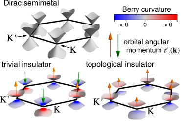
Figure 1: Illustration of the Berry curvature and orbital angular momentum. The surfaces represent the valence and conduction band, while the coloring indicates the Berry curvature. The arrows illustrate the orbital angular momentum of the valence band.

The individual bands possess intrinsic properties which are determined by the band structure topology. An important example of such properties is the OAM. The full description of the OAM and the related orbital magnetization in terms of the Berry phase theory Thonhauser et al. (2005); Xiao et al. (2005) (so-called modern theory of polarization) has been formulated relatively recently. For a band $\alpha$ with spin $\sigma$, the orbital moment is defined as

$$\ell_{z}(\mathbf{k})=\frac{m}{\hbar}\mathrm{Im}\langle\partial_{k_{x}}u_{\mathbf{k}\alpha\sigma}|\hat{h}_{\sigma}(\mathbf{k})-\varepsilon_{\mathbf{k}\alpha}|\partial_{k_{y}}u_{\mathbf{k}\alpha\sigma}\rangle.$$ (2)

This shows that the orbital magnetization $m_{z}(\mathbf{k})=(e/m)\ell_{z}(\mathbf{k})$ is an intrinsic property of the underlying band, related to self-rotation, which can emerge even if no magnetic atoms are present.

The orbital moment (2) transforms exactly as the Berry curvature under symmetry operations, underpinning their tight connection. In particular, in the case where the Berry curvature is primarily due to a valence ($v$) band coupling to a conduction ($c$) band, the OAM becomes proportional to the Berry curvature $\Omega_{v\sigma}(\mathbf{k})$ of the valence band:

$$\ell_{z}(\mathbf{k})=-\frac{m}{\hbar}(\varepsilon_{\mathbf{k}c}-\varepsilon_{\mathbf{k}v})\Omega_{v\sigma}(\mathbf{k})\ .$$ (3)

TRS implies $\Omega_{v\uparrow}(\mathbf{k})=-\Omega_{v\downarrow}(-\mathbf{k})$, while inversion symmetry results in $\Omega_{v\uparrow}(\mathbf{k})=\Omega_{v\uparrow}(-\mathbf{k})$. Hence, in systems possessing both symmetries, $\Omega_{v\uparrow}(\mathbf{k})=-\Omega_{v\downarrow}(\mathbf{k})$ holds; in absence of SOC the Berry curvature and thus the OAM vanishes exactly. Therefore, measuring the momentum-resolved OAM allows to map out the local Berry curvature.

For graphene-like insulating systems, the Berry curvature and the OAM for the three possible scenarios are sketched in Fig. 1. Graphene (neglecting the SOC) possesses inversion symmetry, and respective sublattice sites on the honeycomb lattice are equivalent; hence $\ell_{z}(\mathbf{k})$ is zero in both spin channels, giving rise to a Dirac semimetal. Breaking inversion symmetry – for instance by considering systems with inequivalent atoms on the respective sublattice sites as in hexagonal boron nitride (hBN) – opens a gap and generates a nonzero Berry curvature. The resulting trivial insulator shows OAM at the Dirac points K and K^′ with opposite sign due to TRS. The system is characterized by a nonzero valley Chern number $C_{\mathrm{val}}(K)=-C_{\mathrm{val}}(K^{\prime})=\int_{\mathrm{val}(K)}d\mathbf{k}\,\Omega_{v}(\mathbf{k})/2\pi$, indicating a pronounced valley magnetization Gunawan et al. (2006).

Spin-orbit coupling in graphene-like systems renders them (type-II) $\mathbb{Z}_{2}$ spin Chern insulators Hasan and Kane (2010), according to the Kane-Mele mechanism Kane and Mele (2005a). The bands exhibit an inverted orbital character at K and K^′, respectively, while the TRS is broken for each spin channel individually (even though the system possesses global TRS). Considering the total OAM, the spin Chern number $C_{s}=\pm 1$ indicates a total chiral $L_{z}=\int d\mathbf{k}\,\ell_{z}(\mathbf{k})\neq 0$, with the same magnitude and opposite sign for spin-up and spin-down electrons, respectively.

While optical techniques sensitive to a total chirality – such as magnetic circular dichroism (MCD) – cannot separate out the individual spin channels, advances in spin-resolved ARPES Okuda (2017) (sARPES) enable a selective measurement of spin-up or spin-down photoelectrons. A dichroic sARPES measurement would allow to map out momentum- and spin-resolved OAM properties, which is hard to achieve by other methods. Recent experiments on chiral surface states in TIs Park et al. (2012a) demonstrate the feasibility of detecting circular dichroism in photoemission.

III Circular dichroism in spin- and angle-resolved photoemission

To discuss how the OAM is reflected in ARPES we consider the photoemission intensity as described by Fermi’s Golden Rule in the dipole approximation Schattke and Hove (2008)

$$I(\mathbf{p},\varepsilon_{f})\propto\left|\langle\chi_{\mathbf{p},p_{\perp}}|\hat{\epsilon}\cdot\hat{D}|\psi_{\mathbf{k}\alpha}\rangle\right|^{2}\delta(\varepsilon_{\mathbf{k}\alpha}+\hbar\omega-\varepsilon_{f})\ ,$$ (4)

where $|\psi_{\mathbf{k}\alpha}\rangle$ denotes the Bloch state corresponding to the cell-periodic wave-function $|u_{\mathbf{k}\alpha}\rangle$. The photon energy is given by $\hbar\omega$, and $\varepsilon_{f}=(\mathbf{p}^{2}+p^{2}_{\perp})/2$ is the energy of the photoelectron final state $|\chi_{\mathbf{p},p_{\perp}}\rangle$. The matrix element of the dipole operator $\hat{D}$ and the polarization direction $\hat{\epsilon}$ determine the selection rules. The in-plane momentum $\mathbf{p}$ is identical to the quasi-momentum $\mathbf{k}$ up to a reciprocal lattice vector. We can extend Eq.  (4) to the spin-resolved intensity $I_{\sigma}(\mathbf{p},\varepsilon_{f})$ by assuming a spin-resolved detection of the final states $|\chi_{\mathbf{p},p_{\perp},\sigma}\rangle$, fixing the photoelectron spin $\sigma$.

To detect OAM textures, we exploit the circular dichroism in ARPES. As sketched in Fig. 2(a) we consider the experimental situation, where the probe field is either left-hand (LCP) or right-hand circularly polarized (RCP), with the polarization vector $\hat{\epsilon}^{(\pm)}$ in plane, i. e. normal incident fields. The corresponding ARPES intensities $I^{(\pm)}(\mathbf{k},\varepsilon_{f})$ then define the total (unpolarized) $I_{\mathrm{tot}}(\mathbf{k},\varepsilon_{f})=I^{(-)}(\mathbf{k},\varepsilon_{f})+I^{(+)}(\mathbf{k},\varepsilon_{f})$ and circular dichroism $I_{\mathrm{CD}}(\mathbf{k},\varepsilon_{f})=I^{(-)}(\mathbf{k},\varepsilon_{f})-I^{(+)}(\mathbf{k},\varepsilon_{f})$ signal.

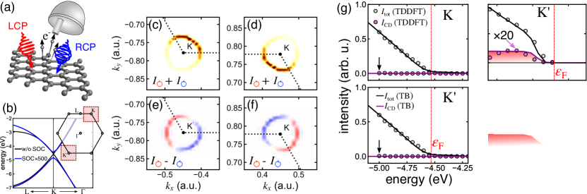
Figure 2: (a) Sketch of the calculation setup: photoemission by left- (LCP) or right- (RCP) hand circularly polarized light, with polarization vector in the plane. (b) Band structure of graphene close to the Dirac point with zero (black line) and enhanced (blue line) SOC, respectively, obtained from density functional theory (DFT). The first Brillouin zone (BZ) of the system with honeycomb lattice is shown in the inset. The shaded boxes indicate the magnified regions shown in (c)–(f). (c) and (d): total ARPES intensity $I_{\mathrm{tot}}(\mathbf{k},\varepsilon_{f})$ (normalized to its maximum value $I_{\mathrm{max}}$) at $\varepsilon_{f}=47$ eV, close to the K and K^′ point, respectively. (e)–(f): corresponding dichroic signal $I_{\mathrm{CD}}(\mathbf{k},\varepsilon_{f})$. (g): Integrated signal (over the shaded regions in (b)) $I_{\mathrm{tot}}$ and $I_{\mathrm{CD}}$ as a function of the binding energy. The black arrow indicates the energy for which the angle-resolved intensities in (c)–(f) are shown. (h) Integrated signal from spin-up electrons (analogous to (g)) for graphene with enhanced SOC.

III.1 Connection to orbital angular momentum

The close connection between the dichroic signal $I_{\mathrm{CD}}(\mathbf{k},\varepsilon_{f})$ and the Berry curvature is already apparent from symmetry considerations. TRS dictates $I_{\mathrm{CD}}(\mathbf{k},\varepsilon_{f})=-I_{\mathrm{CD}}(-\mathbf{k},\varepsilon_{f})$, such that the circular dichroism integrated over the whole Brillouin zone (BZ) vanishes. In addition, a system possessing inversion symmetry results in an exactly vanishing valley-integrated circular dichroism, analogous to the Berry curvature. This argument demonstrates that the breaking of TRS – a characteristic property of Chern insulators – is reflected in a nonzero total circular dichroism.

The manifestation of local OAM chirality in the circular dichroism can be understood intuitively in terms of the wave packet picture, which is also playing a fundamental role in the theory of orbital magnetization Xiao et al. (2010). Instead of a Bloch initial state $|\psi_{\mathbf{k}_{c}\alpha}\rangle$, we can consider a wave packet $|W_{\mathbf{k}\alpha}\rangle$ composed of momenta close to $\mathbf{k}$. Hence, $W_{\mathbf{k}\alpha}(\mathbf{r})$ has a finite spread in real space and properties similar to a molecular orbital. In particular, its OAM is given by $\langle\hat{L}_{z}\rangle=\langle W_{\mathbf{k}\alpha}|\hat{L}_{z}|W_{\mathbf{k}\alpha}\rangle$; in the limit of an infinitely sharp distribution, such that $|W_{\mathbf{k}\alpha}\rangle$ becomes identical to $|\psi_{\mathbf{k}\alpha}\rangle$, one finds $\langle\hat{L}_{z}\rangle=\ell_{z}(\mathbf{k})$. Nonzero $\langle\hat{L}_{z}\rangle$ indicates self-rotation of the wave packet, which will be reflected in the dipole selection rules in the ARPES matrix elements in Eq.  (4).

This picture can be used to obtain a qualitative description of the dichroism, as detailed in Appendix B. Introducing the analogue of a cell-periodic function by $F_{\mathbf{k}\alpha}(\mathbf{r})=e^{-\mathrm{i}\mathbf{k}\cdot\mathbf{r}}W_{\mathbf{k}\alpha}(\mathbf{r})$, its OAM properties can be analyzed by projecting it onto eigenfunctions of $\hat{L}_{z}$: $F_{\mathbf{k}\alpha}(\mathbf{r})=1/\sqrt{2\pi}\sum_{m}e^{\mathrm{i}m\theta}\mathcal{F}_{\mathbf{k}\alpha,m}(s,z)$, where $(s,\theta)$ are the in-plane polar coordinates. Replacing the final states by plane waves (PWs), one can approximate the matrix elements in Eq.  (4) by

$$M^{(\pm)}_{\alpha}(\mathbf{k},p_{\perp})\approx\int^{\infty}_{0}\!ds\,\int^{\infty}_{-\infty}\!dz\,e^{-\mathrm{i}p_{\perp}z}s^{2}\mathcal{F}_{\mathbf{k}\alpha,\mp 1}(s,z)\ .$$ (5)

Therefore, the OAM properties of the initial state are directly reflected in the circular dichroism. In particular, $\langle\hat{L}_{z}\rangle=0$ typically implies $\mathcal{F}_{\mathbf{k}\alpha,+1}(s,z)=\mathcal{F}_{\mathbf{k}\alpha,-1}(s,z)$; hence the circular dichroism vanishes. In Appendix B, we discuss the illustrative example of hBN and analyze the OAM properties in detail.

III.2 Calculation of photoemission spectra

To compute ARPES from first principles one does not need to resort to the approximated one-step model of photoemission like the one of Eq. (4). Instead of using Eq. (4) we employ TDDFT Marques et al. (2011) with the t-SURFFP method De Giovannini et al. (2017) which avoids any reference to explicit final states by directly computing the momentum and energy distribution of the photocurrent created by a specific pulse field and thus allows to compute the intensity directly from the real-time evolution.

While the first-principles approach provides results in excellent agreement with experiments (see below), a more intuitive understanding can be gained by considering a simple model for the direct evaluation of Eq.  (4). The Bloch states are represented by a TB model of atomic orbitals, while replacing the final states $|\chi_{\mathbf{p},p_{\perp}}\rangle$ in this equation by PWs $|\mathbf{p},p_{\perp}\rangle$ eliminates scattering of the photoelectron from the lattice, which allows us to focus on the intrinsic contribution of the Bloch states to the ARPES intensity. The matrix elements in Eq.  (4) are computed in the length gauge, which encodes the selection rules with respect to the LCP or RCP polarization. In what follows, we refer to the resulting model as TB+PW model. Furthermore, an analytical treatment is possible in certain cases, providing a clear physical picture.

The combination of the two methods allows a comprehensive analysis. The details on both methods can be found in Appendix C and D.

IV Results

Here we investigate the three classes of 2D materials represented in Fig. 1, namely the Dirac semimetal, trivial insulator and topological insulator, and identify the distinct features of the circular dichroism in ARPES. The Dirac semimetal we consider is graphene, while hBN exemplifies a trivial insulator. As examples of topological insulators we study bismuthane and graphene with artificially enhanced SOC.

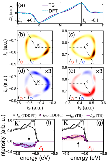
Figure 3: (a) Berry curvature $\Omega_{v}(\mathbf{k})$ of the top valence band, comparing TDDFT and TB result. The OAM amounts to $L_{z}=0.1$ at K and $L_{z}=-0.1$ at K^′. (b)–(c): total ARPES intensity $I_{\mathrm{tot}}(\mathbf{k},\varepsilon_{f})$ at $\varepsilon_{f}=45.811$ eV. (d)–(e): Corresponding circular dichroism. The color coding is analogous to Fig. 2. The integrated signals as a function of the binding energy at K^′ (f) and K (g), respectively.

IV.1 Graphene

We start by discussing ARPES from graphene, which is the prototype of a 2D material. We focus on the regions in the first BZ close to the two inequivalent Dirac points (Fig. 2(b)). The photon energy is fixed at $\hbar\omega=52$ eV. Neglecting the very weak SOC, spin resolution is not required at this point.

Figure 2(c)–(d) shows a typical ARPES cut at fixed $\varepsilon_{f}$, obtained by the t-SURFFP approach. Consistent with experiments Mucha-Kruczyński et al. (2008); Hwang et al. (2011), the prominent dark corridor (region of minimal intensity) is observed in the $\Gamma$–K or $\Gamma$–K^′ direction at this photon energy. The dark corridor is a consequence of destructive interference of the emission from the two sublattice sites Hwang et al. (2011), which can be illuminated by $s$-polarized light Gierz et al. (2011).

The calculated dichroic signal $I_{\mathrm{CD}}(\mathbf{k},\varepsilon_{f})$, shown in Fig. 2(e)–(f), is in very good agreement with experimental data reported in Ref. Gierz et al. (2012). In particular, when following a path perpendicular to the $\Gamma$–K direction, the chiral character is consistent with the experimental data from Ref. Liu et al. (2011). As is apparent from Fig. 2(e)–(f), the valley-integrated circular dichroism vanishes. This is confirmed by both theoretical methods, shown in Fig. 2(g), where we compare the integrated TDDFT results to those of the TB+PW model for an integration range corresponding to the two shaded regions in Fig. 2(b), finding excellent agreement. Hence, the dichroic properties provide a direct proof of the vanishing Berry curvature.

IV.2 Hexagonal boron nitride

We now turn to the paradigmatic case of a trivial insulator with broken inversion symmetry (as sketched in Fig. 1) by studying single-layer hBN. Similar to graphene, hBN is a $\pi$-conjugated system dominated by $p_{z}$ orbitals on the sublattice sites with a large ionic-like band gap. The Berry curvature becomes finite and very pronounced around the K and K^′ points. Comparing $\Omega_{v}(\mathbf{k})$ of the top valence band within the TB model and the first-principles calculation (Fig. 3(a)), the excellent agreement indicates that the orbital mixing of the top valence and bottom conduction band – of predominant $p_{z}$ orbital character – gives the main contribution to $\Omega_{v}(\mathbf{k})$. Hence, Berry curvature and OAM $\ell_{z}(\mathbf{k})$ are are proportional to each other, c. f. Eq.  (3). The valley-integrated OAM is $L_{z}\approx\pm 0.1$ with opposite sign at K and K^′, respectively (Fig. 3(a)). We have also explictly evaluated wave packets and the associated OAM in Appendix B. The prediction of the dichroism from Eq.  B.2 is qualitatively in line with the calculated circular dichroism in Fig. 3(d)–(e).

The valley-resolved measurement provided by ARPES – as opposed to MCD Souza and Vanderbilt (2008) – allows to trace the valley OAM Yao et al. (2008). Because of the direct link to the local Berry curvature (Eq.  (3)) this provides a way of measuring the valley Chern number.

Figure 3(b)–(c) shows the unpolarized signal $I_{\mathrm{tot}}(\mathbf{k},\varepsilon_{f})$ for hBN close to the K and K^′ points. Note the suppression of the dark corridor, which is due to the incomplete destructive interference. The corresponding circular dichroism (Fig. 3(d)–(e)) shows – following the behavior of $\Omega_{v}(\mathbf{k})$ and the OAM – an opposite character at the two inequivalent Dirac points. While irradiating with LCP light results in a much larger probability of creating a photoelectron in the vicinity of the K point, RCP light dominates the emission from the region around K^′. Integrating the momentum-resolved signals yields a clear picture (Fig. 3(f)–(g)). The first-principles TDDFT results are qualitatively well reproduced by the TB+PW model, underpinning the intrinsic character of the dichroism.

IV.3 Bismuthane

To demonstrate the generic character of the connection between the Berry curvature and circular dichroism, we consider single-layer hydrogenated bismuthane (BiH), see Fig. 4(a). Bismuth on the hexagonal lattice is one of most promising candidates for realizing 2D TIs Li et al. (2018); Reis et al. (2017) due to its strong intrinsic SOC. A monolayer of hexagonal Bismuth has been experimentally characterized on a SiC substrate Reis et al. (2017). Free-standing bismuth has $p_{x}$, $p_{y}$ and $p_{z}$ orbitals contributing to the bands close to the Fermi energy; removing the $p_{z}$ orbitals from this energy range has been identified as a key mechanism Li et al. (2018). The hydrogen atoms fulfill exactly this purpose. The system is slightly buckled, but still possesses inversion symmetry, such that the spin states are degenerate.

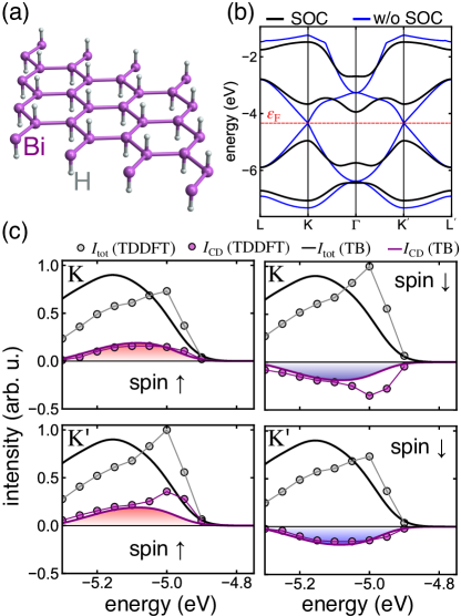
Figure 4: (a) Lattice structure of hexagonal BiH. (b) Band structure of BiH (obtained from DFT), fully including SOC (black) and to comparing to the case without any SOC (blue lines). (c) Integrated dichroic signal as in Fig. 2 for spin-up (left) and spin-down electrons (right panels) at K (upper) and K^′ (lower panels), respectively.

Artificially turning off the SOC, turns BiH into a Dirac semimetal (Fig. 4(b)), while the SOC opens a large gap of $\simeq 800$ meV at K and $K^{\prime}$.

Due to the TRS, the Berry curvature (see Fig. 1) is opposite for spin-up and spin-down electrons, respectively. Hence, sAPRES is required to distinguish the spin species. Fig. 4(c) shows the integrated ARPES signals for both spin channels, in analogy to the non-spin resolved case of Fig. 3(f) and (g). We are focusing on the top valence band. As expected from the case of the TI in Fig. 1, the Berry curvature has the sign at both K and K^′, and so has the OAM. The behavior is opposite for spin-up and spin-down, respectively; note that the global TRS implies $I_{\mathrm{CD},\uparrow}(\mathbf{k},\varepsilon_{f})=-I_{\mathrm{CD},\downarrow}(-\mathbf{k},\varepsilon_{f})$. Hence, the integrated circular dichroism has the same sign, confirming that BiH is a spin Chern insulator. To corroborate the topological nature of the dichroism, we have switched off the SOC within the TB+PW model. We find vanishing valley-integrated dichroism, which is consistent with the signatures of a Dirac semimetal like graphene.

As a second example of a spin Chern insulator we can consider graphene. Even though SOC is very weak in graphene, it theoretically also renders graphene a spin Chern insulator Hasan and Kane (2010), so it is instructive in this context to study graphene with SOC. However, the SOC induced gap of $\sim 25$ $\mu$eV Konschuh et al. (2010) is very small, so that graphene in practice behaves like a trivial material, as discussed above. In order to reveal the dichroic signature of the topologically nontrivial phase, we artificially enhance the SOC by a factor of 500. This allows to directly observe the impact of the Kane-Mele mechanism Kane and Mele (2005b) on the circular dichroism. The opening of the topological gap is shown in Fig. 2(b). The integrated intensities in Fig. 2(b) show a very good agreement between the full TDDFT calculations and the TB+PW calculations for the unpolarized intensity $I_{\mathrm{tot}}$. The circular dichroism is overestimated by the TB+PW model by a factor of $\sim 20$. This indicates that the circular dichroism due to scattering effects (which are missing in the TB+PW model) is competing with the intrinsic dichroism. Nevertheless, the qualitative behavior in both approaches clearly shows a non-vanishing total circular dichroism – and thus reveals a topologically nontrivial state.

IV.4 Universal phase diagram for graphene-like systems

The examples for the three cases of $\pi$-conjugate systems discussed above – Dirac semimetal (graphene), trivial insulator (hBN) and topological insulator (graphene with SOC) – can all be described on the TB level by the Haldane model Haldane (1988). The Haldane model is characterized by the gap parameter $M$, nearest-neighbor hopping $J$, next-nearest neighbor hopping $J^{\prime}$, and the associated phase $\phi$. For $M=2.14J$, $J^{\prime}=0$, $\phi=0$, the TB model of hBN is recovered, while $M=0$, $J^{\prime}=-0.0473J$, $\phi=\mathrm{arg}(J^{\prime}-i\lambda)$ corresponds to the TB model for graphene with SOC strength $\lambda$ Kane and Mele (2005b); Wang et al. (2013a).

The good qualitative agreement between the ab initio TDDFT data and the results from the TB+PW model in all considered cases demonstrates the predictive power of the simplified description. Hence, the TB+PW approach may be used to explore the full phase diagram of the Haldane model, providing a comprehensive picture of the circular dichroism in graphene-like systems. For our analysis, we have adopted the parameters and atomic orbitals from graphene, but replaced the TB Hamiltonian by the Haldane model. We have computed the $\mathbf{k}$-integrated (over the region shown in Fig. 2(b)) signal $I_{\mathrm{CD}}(\mathrm{K}^{(\prime)},\varepsilon)$, as in Fig. 2, and in addition integrated over the binding energy $\varepsilon$. The such integrated (but valley-resolved) dichroic signal $S_{\mathrm{CD}}(\mathrm{K}^{(\prime)})=\int\!d\varepsilon\,I_{\mathrm{CD}}(\mathrm{K}^{(\prime)},\varepsilon)$ is shown in Fig. 5 (a)–(b).

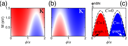
Figure 5: Energy- and valley-integrated circular dichroism $S_{\mathrm{CD}}$ around the K (a) and K^′ (b) valley, respectively, as a function of the phase $\phi$ and gap parameter $M$. (c): asymmetry signal $\Delta S_{\mathrm{CD}}$ (see text): red color corresponds to $\Delta S_{\mathrm{CD}}=1$, blue to $\Delta S_{\mathrm{CD}}=-1$, and white to $\Delta S_{\mathrm{CD}}=0$. The dashed lines represent the critical gap $M_{\mathrm{crit}}(\phi)$, for which $M>M_{\mathrm{crit}}(\phi)$ turns the system into a trivial insulator. The Chern numbers $C$ are given for each phase. The parameters are analogous to graphene, with $J^{\prime}=0.1J$.

As Fig. 5(a)–(b) demonstrates, the system exhibits a total dichroism (dominated by LCP light) for $\phi<\pi$ and small enough $M$. For larger $M$, the dichroism stays positive around the K point, while it becomes negative at K^′. The behavior for $\phi>\pi$ is inverted. This suggests the following measurement strategy: if both $S_{\mathrm{CD}}(\mathrm{K})>0$ and $S_{\mathrm{CD}}(\mathrm{K}^{\prime})>0$, the system represents a Chern insulator. Similarly, $S_{\mathrm{CD}}(\mathrm{K})<0$ and $S_{\mathrm{CD}}(\mathrm{K}^{\prime})<0$ should correspond to a Chern insulator with opposite Chern number. The case $S_{\mathrm{CD}}(\mathrm{K})S_{\mathrm{CD}}(\mathrm{K}^{\prime})<0$ indicates a topologically trivial phase. All these cases can be captured by defining $\Delta S_{\mathrm{CD}}=(\mathrm{sign}[S_{\mathrm{CD}}(\mathrm{K})]+\mathrm{sign}[S_{\mathrm{CD}}(\mathrm{K}^{\prime})])/2$, which is presented in Fig. 5(c) and compared to the topological phase diagram of the Haldane model.

Fig. 5(c) demonstrates a close relation between the circular dichroism and the topological state, since the region $\Delta S_{\mathrm{CD}}=1$ ($\Delta S_{\mathrm{CD}}=-1$) is almost identical to the parameter space with Chern number $C=1$ ($C=-1$). In contrast, the topologically trivial regime ($C=0$) is characterized by $\Delta S_{\mathrm{CD}}=0$. The corresponding topological phase diagram shown in Fig. 5(c) is also consistent with the previous results: the hBN case would be recovered for large enough $M$ (outside the plotted range), while the TB model for graphene with SOC for the spin-up (spin-down) species is equivalent to the Haldane model with $\phi=17^{\circ}$ ($\phi=343^{\circ}$).

The good agreement between the properties of the CD and the topological phase diagram can be further supported by an analytical evaluation of the TB+PW model (detailed in Appendix E). Assuming unperturbed atomic orbitals, we explictly calculate the matrix elements $M^{(\pm)}(\mathbf{k},p_{\perp})=\langle\mathbf{k},p_{\perp}|\hat{\epsilon}^{(\pm)}\cdot\mathbf{r}|\psi_{\mathbf{k}v}\rangle$ and the asymmetry $\Delta\mathcal{M}(\mathbf{k},p_{\perp})=|M^{(+)}(\mathbf{k},p_{\perp})|^{2}-|M^{(-)}(\mathbf{k},p_{\perp})|^{2}$. This quantity is, up to the energy conservation in Eq.  (4), equivalent to the dichroic ARPES intensity. Under these assumptions one can derive

$$\Delta\mathcal{M}(\mathbf{k},p_{\perp})\propto\sigma_{z}(\mathbf{k})[\mathbf{k}\times\boldsymbol{\tau}]_{z}\,\widetilde{\varphi}(k,p_{\perp})\partial_{k}\widetilde{\varphi}(k,p_{\perp})\ ,$$ (6)

where $\boldsymbol{\tau}$ is the vector connecting the sublattice sites, while $\widetilde{\varphi}(k,p_{\perp})$ is the Fourier transform of the atomic $p_{z}$ wave function (depending on the modulus $k=|\mathbf{k}|$ only).

The most important term is the orbital pseudospin $\sigma_{z}(\mathbf{k})=P_{\mathrm{A}}(\mathbf{k})-P_{\mathrm{B}}(\mathbf{k})$, measuring the difference in orbital occupation $P_{\mathrm{A,B}}(\mathbf{k})$ of the sublattice sites. In a topologically trivial state, only the lower-energy site is predominantly occupied (for instance, the nitrogen site in hBN), hence $\sigma_{z}(\mathbf{k})<0$ across the whole BZ. Therefore, Eq.  (6) yields opposite signs at $\mathbf{k}=\mathrm{K}$ and $\mathbf{k}=\mathrm{K}^{\prime}$. In contrast, in a topologically nontrivial state the orbital inversion leads to a change of sign of $\sigma_{z}(\mathbf{k})$ in the BZ. In particular, $\sigma_{z}(\mathrm{K})$ and $\sigma_{z}(\mathrm{K}^{\prime})$ must have opposite signs. Therefore, the asymmetry (6) has the same sign at both K and K^′. Hence, the analytical model clearly shows that the total dichroism changes at a topological phase transition.

V Discussion and Conclusion

We have presented a detailed investigation of ARPES and, in particular, the circular dichroism from 2D graphene-like systems. The results were obtained by first-principles calculations of the ARPES intensity based on TDDFT, and complemented by the analysis of a simple TB model.

In general, circular dichroism in photoemission can have multiple origins. For instance, interference and scattering effects from the lattice give rise to distinct dichroism. However, in a system possessing both inversion and TRS (like graphene without SOC), the valley-integrated CD vanishes. Our main focus was not the dichroism related to lattice effects, but that originating from an intrinsic property of the underlying band. In this context, hBN is an ideal test system. In this case, the broken inversion symmetry gives rise to a pronounced Berry curvature and associated OAM. The distinct OAM states at the two inequivalent Dirac points directly translates into a pronounced valley-integrated dichroism. This is underpinned by the TB model. We stress that the connection between the OAM and the dichroism is generic and not restricted to graphene-like systems, as confirmed by the example of single-layer BiH. A pronounced valley dichroism can also be expected in monolayer transition metal dichalcogenides of the type MX₂ Bertoni et al. (2016). Hence, dichroic ARPES provides an excellent tool for studying the OAM and valley topological effects. We stress that the sensitivity to the local Berry curvature is a distinct feature of (spin-resolved) ARPES with its resolution in momentum space.

The example of BiH shows that the TRS breaking associated with the restriction to one spin species results in total dichroism. Analogous effects are present in graphene with enhanced SOC. Hence, measuring circular dichroism from a 2D system allows to directly determine its topological property, even for a TI with overall TRS. The key aspect is the spin resolution provided by spin-resolved ARPES. This is in contrast to, for instance, optical absorption, which could not distiniguish the spin species and would thus result in zero dichroism for spin Chern insulators, which constitute the majority of existing 2D TIs. Hence, measuring circular dichroism in spin-resolved ARPES provides a powerful tool for the identification of TIs.

Furthermore, the extension of ARPES to the time domain (tARPES) Schmitt et al. (2008); Wang et al. (2013b); Sentef et al. (2013), offers a new way of tracing and defining transient topological phenomena. For instance, the build-up of light-induced topological states Kitagawa et al. (2011); Sentef et al. (2015); Dahlhaus et al. (2015); Claassen et al. (2016); Hübener et al. (2017); Topp et al. (2018); Claassen et al. (2018); McIver et al. (2018) should be observable with tARPES in real time. This is particularly important as laser-heating effects typically lead to thermalization at high temperature, where the Hall conductance is not quantized Schüler et al. (2018); Sato et al. (2019). In contrast, the energy selectivity of ARPES allows to identify the topological character of the individual bands, thus providing a conclusive result even in highly excited systems.

Appendix A Spin-orbit coupling effects in graphene and BiH

In this appendix we show that $S_{z}$ as approximate quantum number for the systems with SOC which we discuss in this work. To this end, we have solved the Kohn-Sham equations including the SOC (numerical details in Appendix C), treating the Bloch wave-functions $|\Psi_{\mathbf{k}\alpha}\rangle$ as general spinors. This allows for calculating the expectation value $S_{z}(\mathbf{k})=\langle\Psi_{\mathbf{k}\alpha}|\hat{s}_{z}|\Psi_{\mathbf{k}\alpha}\rangle$, where $\hat{s}_{z}=(\hbar/2)\hat{\sigma}_{z}$ denotes the operator of the z-projection of the spin.

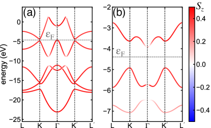
Figure 6: Spin expectation value $S_{z}(\mathbf{k})$ of the predominantly spin-up bands for (a) graphene with enchanced SOC, and (b) BiH. The color bar is in units of $\hbar$.

Fig. 6 shows $S_{z}(\mathbf{k})$ for both graphene with enhanced SOC as well as for BiH with full intrinsic SOC. We have focused on the bands with predominant spin-up character close to the Fermi energy. As Fig. 6 demonstrates, $S_{z}(\mathbf{k})$ is very close to $+\hbar/2$ in the vicinity of the K and K^′ point for the top valence band and most parts of the bottom conduction band. Hence, $S_{z}$ can be regarded as good quantum number, justifying the block-diagonal structure of the Hamiltonian (1).

Appendix B wave packet picture

To understand the self-rotation and the associated orbital magnetic moment, we employ the wave packet picture Ashcroft and Mermin (1976). Let us consider a wave packet with respect to band $\alpha$ of the form

$$W_{\mathbf{k}\alpha}(\mathbf{r})=\int\!d\mathbf{q}\,a(\mathbf{k},\mathbf{q})\psi_{\mathbf{q}\alpha}(\mathbf{r})=\int\!d\mathbf{q}\,a(\mathbf{k},\mathbf{q})e^{\mathrm{i}\mathbf{q}\cdot\mathbf{r}}u_{\mathbf{q}\alpha}(\mathbf{r})\ .$$ (7)

For computing ARPES matrix elements, it is convenient to introduce an analogue of cell-periodic functions by $F_{\mathbf{k}\alpha}(\mathbf{r})=e^{-\mathrm{i}\mathbf{k}\cdot\mathbf{r}}W_{\mathbf{k}\alpha}(\mathbf{r})$. The envelope function $a(\mathbf{k},\mathbf{q})$ represents a narrow distribution around a central wave vector $\mathbf{k}$; its precise functional form does not play a role. Denoting the center of the wave packet by

$$\mathbf{r}_{c}=\langle W_{\mathbf{k}\alpha}|\mathbf{r}|W_{\mathbf{k}\alpha}\rangle=\langle F_{\mathbf{k}\alpha}|\mathbf{r}|F_{\mathbf{k}\alpha}\rangle\ ,$$ (8)

one defines Xiao et al. (2005) the angular momentum as

$$\langle\hat{\mathbf{L}}\rangle=\langle W_{\mathbf{k}\alpha}|(\mathbf{r}-\mathbf{r}_{c})\times\hat{\mathbf{p}}|W_{\mathbf{k}\alpha}\rangle=\langle F_{\mathbf{k}\alpha}|(\mathbf{r}-\mathbf{r}_{c})\times\hat{\mathbf{p}}|F_{\mathbf{k}\alpha}\rangle\ ,$$ (9)

where $\hat{\mathbf{p}}$ denotes the momentum operator. The wave packet representation of OAM (9) naturally leads to the so-called modern theory of magnetization Aryasetiawan and Karlsson in the limit of $a(\mathbf{k},\mathbf{q})\rightarrow\delta(\mathbf{q}-\mathbf{k})$.

B.1 Expansion in eigenfunctions of angular momentum

To quantify the OAM, we expand the wave packet $F_{\mathbf{k}\alpha}(\mathbf{r})$ onto eigenfunctions of the OAM $\hat{L}_{z}$:

$$F_{\mathbf{k}\alpha}(\mathbf{r})=\frac{1}{\sqrt{2\pi}}\sum_{m}\mathcal{F}_{\mathbf{k}\alpha,m}(s,z)e^{\mathrm{i}m\theta}\ .$$ (10)

Here, $\theta$ is the angle measured in the 2D plane, taking $\mathbf{r}_{c}$ as the origin, while $s=|\mathbf{r}_{\parallel}-\mathbf{r}_{c}|$ is the corresponding distance. Inserting the expansion (10) into Eq.  (9) yields the simple expression

$$\langle\hat{L}_{z}\rangle =\sum_{m}m\int^{\infty}_{0}\!ds\,s\int^{\infty}_{-\infty}\!dz\,\left|\mathcal{F}_{\mathbf{k}\alpha,m}(s,z)\right|^{2}$$

$$\equiv\sum_{m}mP_{\mathbf{k}\alpha}(m)\ .$$ (11)

Hence, a nonzero orbital angular momentum projection in the $z$ direction can be associated with an imbalance of the occupation of angular momentum states $P_{\mathbf{k}\alpha}(m)$.

B.2 Photoemission matrix elements

Approximating the initial Bloch states $|\psi_{\mathbf{k}\alpha}\rangle$ by the wave packet state $|W_{\mathbf{k}\alpha}\rangle$ and the final states by plane waves, the dipole matrix elements are given by

$$M^{(\pm)}_{\alpha}(\mathbf{p},p_{\perp}) =\int\!d\mathbf{r}_{\parallel}\!\int^{\infty}_{-\infty}\!dz\,e^{-\mathrm{i}\mathbf{p}\cdot\mathbf{r}_{\parallel}}e^{-\mathrm{i}p_{\perp}z}(x\pm\mathrm{i}y)W_{\mathbf{k}\alpha}(\mathbf{r})$$

$$=\frac{1}{\sqrt{2}}\int\!d\mathbf{r}_{\parallel}\!\int^{\infty}_{-\infty}\!dz\,e^{-\mathrm{i}(\mathbf{p}-\mathbf{k})\cdot\mathbf{r}_{\parallel}}e^{-\mathrm{i}p_{\perp}z}(x\pm\mathrm{i}y)F_{\mathbf{k}\alpha}(\mathbf{r})\ .$$ (12)

Now we insert the angular-momentum representation (10) and the plane-wave expansion around $\mathbf{r}_{c}$

$$e^{\mathrm{i}(\mathbf{p}-\mathbf{k})\cdot\mathbf{r}_{\parallel}}=e^{\mathrm{i}(\mathbf{p}-\mathbf{k})\cdot\mathbf{r}_{c}}\sum_{m}\mathrm{i}^{m}J_{m}(|\mathbf{p}-\mathbf{k}|s)e^{\mathrm{i}m(\theta-\theta(\mathbf{p},\mathbf{k}))}\ ,$$

where $\theta(\mathbf{p},\mathbf{k})$ is the angle defining the direction of $\mathbf{p}_{\parallel}-\mathbf{k}$, into Eq.  (B.2). Thus, we can express the matrix elements as

$$M^{(\pm)}_{\alpha}(\mathbf{p},p_{\perp})=e^{\mathrm{i}(\mathbf{p}-\mathbf{k})\cdot\mathbf{r}_{c}}\sum_{m}(-\mathrm{i})^{m\pm 1}e^{\mathrm{i}(m\pm 1)\theta(\mathbf{p},\mathbf{k})}$$

$$\times\int^{\infty}_{0}\!ds\,\int^{\infty}_{-\infty}\!dz\,e^{-\mathrm{i}p_{\perp}z}J_{m\pm 1}(|\mathbf{p}-\mathbf{k}|s)s^{2}\mathcal{F}_{\mathbf{k}\alpha,m}(s,z)\ .$$ (13)

Assuming the distribution $a(\mathbf{k},\mathbf{q})$ to be sufficiently narrow, such that Bloch states are recovered, the energy conservation implies $\mathbf{p}\approx\mathbf{k}$. As $J_{m}(x)\rightarrow 0$ for $x\rightarrow 0$ with $m\neq 0$, only the term with $m=0$ contributes to the sum in Eq.  (B.2). The dominant matrix element simplifies to

$$M^{(\pm)}_{\alpha}(\mathbf{k},p_{\perp})=\int^{\infty}_{0}\!ds\,\int^{\infty}_{-\infty}\!dz\,e^{-\mathrm{i}p_{\perp}z}s^{2}\mathcal{F}_{\mathbf{k}\alpha,\mp 1}(s,z)\ .$$ (14)

This expression demonstrates that the asymmetry of OAM eigenstates with $m=\pm 1$ determine the circular dichroism.

B.3 Illustration for hBN

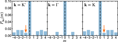
Figure 7: Weights of the projections onto OAM eigenfunctions according to Eq.  (10) for the TB model of hBN. The width of the distribution is $\Delta k=0.025$ in reduced coordinates. The arrows indicate the dominant contribution for the matrix elements (14).

In order to illustrate the discussion above, we have constructed Bloch wave packets according to Eq.  (7), choosing a distibution function $a(\mathbf{k},\mathbf{q})=a_{0}\exp[-(\mathbf{q}-\mathbf{k})^{2}/(2\Delta k^{2})]$ ($a_{0}$ is a normalization constant). The underlying Bloch wave functions are constructed using the TB model for hBN.

We have computed the projection onto planar OAM eigenfunctions (Eq.  (10)) and the corresponding weights $P_{\mathbf{k}\alpha}(m)=$ for the valence band ($\alpha=v$), as presented in Fig. (7). As Fig. (7) demonstrates, the OAM eigenstate $m=-1$ ($m=+1$) dominates at $\mathbf{k}=\mathrm{K}^{\prime}$ ($\mathbf{k}=\mathrm{K}$). At $\mathbf{k}=\mathrm{K}^{\prime}$, we expect photoelectrons emitted by RCP light – this is in line with Fig. 3. The behavior at $\mathbf{k}=\mathrm{K}$ is reversed. In contrast, at $\mathbf{k}=\Gamma$ the weights are symmetric. Hence, vanishing dichroism is expected around the $\Gamma$-point; we have confirmed this behavior by explicitly calculating the circular dichroism within the full TB+PW model.

Appendix C Ab-initio ARPES simulations: numerical details

The evolution of the electronic structure under the effect of external fields was computed by propagating the Kohn-Sham (KS) equations in real space and real time within TDDFT as implemented in the Octopus code Marques et al. (2003); Castro et al. (2006); Andrade et al. (2015); noa . We solved the KS equations in the local density approximation (LDA) Perdew (1981) with semi-periodic boundary conditions. For all the systems considered, we used a simulation box of 120 $a_{0}$ along the non-periodic dimension and the primitive cell on the periodic dimensions with a grid spacing of 0.36 $a_{0}$, and sampled the Brillouin zone with a 12$\times$12 k-point grid. We modeled graphene with a lattice parameter of 6.202 $a_{0}$ and hBN with 4.762 $a_{0}$. Time and spin-resolved ARPES was calculated by recording the flux of the photoelectron current over a surface placed 30 $a_{0}$ away from the system with the t-SURFFP method De Giovannini et al. (2017); De Giovannini (2018) – the extension of t-SURFF Scrinzi (2012); Wopperer et al. (2017) to periodic systems. All calculations were performed using fully relativistic HGH pseudopotentials Hartwigsen et al. (1998).

Appendix D Tight-binding modelling

D.1 Tight-binding representation of initial states

Within the TB model, we approximate the Bloch states $\psi_{\mathbf{k}\alpha}(\mathbf{r})$ by

$$\psi_{\mathbf{k}\alpha}(\mathbf{r}) =\frac{1}{\sqrt{N}}\sum_{\mathbf{R}}e^{\mathrm{i}\mathbf{k}\cdot\mathbf{R}}\phi_{\mathbf{k}\alpha}(\mathbf{r}-\mathbf{R})$$

$$=\frac{1}{\sqrt{N}}\sum_{\mathbf{R}}\sum_{j}C_{\alpha j}(\mathbf{k})e^{\mathrm{i}\mathbf{k}\cdot(\mathbf{R}+\mathbf{t}_{j})}w_{j}(\mathbf{r}-\mathbf{R})\ .$$ (15)

Here, we are employing the convention where the phase factor $e^{\mathrm{i}\mathbf{k}\cdot\mathbf{t}_{j}}$ ($\mathbf{t}_{j}$ denotes the sublattice site positions) is directly included in the definition (D.1) of the Bloch states.

For all considered systems, we have constructed a nearest-neighbour (NN) TB model and fitted the onsite and hopping energy to the respective bandstructure of the DFT calculation. For graphene with enhanced SOC, we have used the next-NN model from Ref. Kane and Mele (2005b) and fitted the corresponding SOC parameter. For BiH, we used the effective TB Hamiltonian from Ref. Li et al. (2018) for the subset of $p_{x}$ and $p_{y}$ orbitals. In all cases, the bandstructure obtained by the TB models matches the DFT energies close to the K and K^′ point very well.

The TB Wannier orbitals are approximated as

$$w^{\gamma}_{j}(\mathbf{r})=C_{j}\mathbf{u}_{\gamma}\cdot(\mathbf{r}-\mathbf{t})_{j}\exp\left[-\alpha_{j}(\mathbf{r}-\mathbf{t}_{j})^{2}\right]\ ,$$ (16)

where $\mathbf{u}_{\gamma}$ is the unit vector in the direction $\gamma=x,y,z$. The parameters $C_{j}$ and $\alpha_{j}$ are fitted to atomic orbitals.

D.2 Matrix elements

To further simplify the analysis, we approximate the final states as plane-waves (PW). The cell-periodic part $\tilde{\chi}_{\mathbf{p},p_{\perp}}(\mathbf{r})=e^{-\mathrm{i}\mathbf{k}\cdot\mathbf{r}}\chi_{\mathbf{p},p_{\perp}}(\mathbf{r})$ thus reduces to $\tilde{\chi}_{\mathbf{p},p_{\perp}}(\mathbf{r})=N^{-1/2}e^{\mathrm{i}p_{\perp}z}$, where $N$ is the normalization as in the Wannier representation (D.1).

Due to the periodicity of both the initial and final states, the matrix element entering Eq.  (4),

$$M_{\alpha}(\mathbf{p},p_{\perp})=\langle\chi_{\mathbf{p},p_{\perp}}|\hat{\epsilon}\cdot\mathbf{r}|\psi_{\mathbf{k}\alpha}\rangle,$$ (17)

is only nonzero if $\mathbf{p}=\mathbf{k}+\mathbf{G}$, where $\mathbf{G}$ is a reciprocal lattice vector. Here, we focus on ARPES from the first BZ, so that $\mathbf{G}=0$.

To evaluate the photoemission matrix element in the length gauge, we employ the identity

$$\mathbf{r}\psi_{\mathbf{k}\alpha}(\mathbf{r})=\mathrm{i}e^{\mathrm{i}\mathbf{k}\cdot\mathbf{r}}\nabla_{\mathbf{k}}u_{\mathbf{k}\alpha}(\mathbf{r})-\mathrm{i}\nabla_{\mathbf{k}}\psi_{\mathbf{k}\alpha}(\mathbf{r})\ ,$$

which transforms the dipole operator into a cell-periodic expression. Inserting the Wannier representation (D.1) into Eq.  (17), we find for the matrix elements

$$M_{\alpha}(\mathbf{k},p_{\perp}) =\frac{\mathrm{i}}{\sqrt{N}}\sum_{\mathbf{R}}\int\!\mathrm{d}\mathbf{r}\,\tilde{\chi}^{*}_{\mathbf{k}p_{\perp}}(\mathbf{r})\hat{\epsilon}\cdot\nabla_{\mathbf{k}}\left[e^{-\mathrm{i}\mathbf{k}\cdot(\mathbf{r}-\mathbf{R})}\phi_{\mathbf{k}\alpha}(\mathbf{r}-\mathbf{R})\right]-\frac{\mathrm{i}}{N}\sum_{\mathbf{R}}\int\!\mathrm{d}\mathbf{r}\,\chi^{*}_{\mathbf{k}p_{\perp}}(\mathbf{r})\hat{\epsilon}\cdot\nabla_{\mathbf{k}}\left[e^{\mathrm{i}\mathbf{k}\cdot\mathbf{R}}\phi_{\mathbf{k}\alpha}(\mathbf{r}-\mathbf{R})\right]$$

$$=\sqrt{N}\int\!\mathrm{d}\mathbf{r}\,\chi^{*}_{\mathbf{k}p_{\perp}}(\mathbf{r})\hat{\epsilon}\cdot\mathbf{r}\phi_{\mathbf{k}\alpha}(\mathbf{r})-\frac{1}{\sqrt{N}}\sum_{\mathbf{R}}\hat{\epsilon}\cdot\mathbf{R}\int\!\mathrm{d}\mathbf{r}\,\chi^{*}_{\mathbf{k}p_{\perp}}(\mathbf{r})\phi_{\mathbf{k}\alpha}(\mathbf{r})\ .$$ (18)

The derivation is analogous to Ref. Park et al. (2012b). The second term in Eq.  (18) vanishes.

Note that the origin $\mathbf{r}_{0}$ from which the dipole is measured ($\mathbf{r}\rightarrow\mathbf{r}-\mathbf{r}_{0}$) is arbitrary if exact scattering states $|\chi_{\mathbf{p},p_{\perp}}\rangle$ are used. However, within the PW approximation, the initial and final states are not exactly orthogonal, which results in a slight dependence on $\mathbf{r}_{0}$. Here, we consistently choose $\mathbf{r}_{0}=(\mathbf{t}_{B}-\mathbf{t}_{A})/2$, where $j=A,B$ denotes the sublattice sites. This choice encodes as many symmetries as possible and leads to a very good agreement of the ARPES intensity between TDDFT and the TB approach.

Defining the Fourier transformed Wannier orbitals by

$$\varphi_{j}(\mathbf{k},p_{\perp})=\int\!\mathrm{d}\mathbf{r}\,e^{-\mathrm{i}\mathbf{k}\cdot\mathbf{r}}e^{-\mathrm{i}p_{\perp}z}w_{j}(\mathbf{r})\ ,$$ (19)

the matrix elements can be expressed via

$$M_{\alpha}(\mathbf{k},p_{\perp})=\mathrm{i}\sum_{j}C_{\alpha j}(\mathbf{k})e^{\mathrm{i}\mathbf{k}\cdot\mathbf{t}_{j}}\hat{\epsilon}\cdot\left[\mathrm{i}\nabla_{\mathbf{k}}-\mathbf{r}_{0}\right]\varphi_{j}(\mathbf{k},p_{\perp})\ .$$ (20)

Appendix E Pseudospin picture

In this appendix we demonstrate that the circular dichroism for $\pi$-conjugate systems like graphene and hBN is directly related to the orbital pseudospin. This provides a clear link to a topological phase transition, which is characterized by a sign change of the pseudospin in the BZ.

The starting point is the expression (20) for the matrix element in the length gauge. The Fourier transformation of the Wannier orbital centered around $\mathbf{t}_{j}$ can be conveniently expressed as $\varphi_{j}(\mathbf{k},p_{\perp})=e^{-\mathrm{i}\mathbf{k}\cdot\mathbf{t}_{j}}\widetilde{\varphi}_{j}(\mathbf{k},p_{\perp})$. In particular, if the Wannier orbital $w_{j}(\mathbf{r})$ is radially symmetric around $\mathbf{t}_{j}$ and symmetric or antisymmetric along the $z$-axis, $\widetilde{\varphi}_{j}(\mathbf{k},p_{\perp})$ becomes a purely real or imaginary function. Simplifying Eq.  (20) in this way, we obtain

$$M_{\alpha}(\mathbf{k},p_{\perp})=\hat{\epsilon}\cdot\sum_{j}C_{\alpha j}(\mathbf{k})(\mathbf{t}_{j}-\mathbf{r}_{0}+\mathrm{i}\nabla_{\mathbf{k}})\widetilde{\varphi}_{j}(\mathbf{k},p_{\perp})\ .$$

The difference of the modulus squared matrix elements upon inserting $\hat{\epsilon}^{(\pm)}$ yields

$$\Delta\mathcal{M}_{\alpha}(\mathbf{k},p_{\perp}) \equiv\left|M^{(+)}_{\alpha}(\mathbf{k},p_{\perp})\right|^{2}-\left|M^{(-)}_{\alpha}(\mathbf{k},p_{\perp})\right|^{2}$$

$$=2\mathrm{Im}\sum_{j,l}C_{\alpha j}(\mathbf{k})C^{*}_{\alpha l}(\mathbf{k})\left[[(\mathbf{t}_{j}-\mathbf{r}_{0})\widetilde{\varphi}_{j}(\mathbf{k},p_{\perp})+\mathrm{i}\nabla_{\mathbf{k}}\widetilde{\varphi}_{j}(\mathbf{k},p_{\perp})\right]\times\left[(\mathbf{t}_{l}-\mathbf{r}_{0})\widetilde{\varphi}^{*}_{l}(\mathbf{k},p_{\perp})-\mathrm{i}\nabla_{\mathbf{k}}\widetilde{\varphi}^{*}_{l}(\mathbf{k},p_{\perp})\right]\ ,$$ (21)

where we take the $z$ component of the vector product. Further evaluating Eq.  (E), the matrix element asymmetry can be decomposed into two terms

$$\Delta\mathcal{M}_{\alpha}(\mathbf{k},p_{\perp})=\Delta\mathcal{M}^{(1)}_{\alpha}(\mathbf{k},p_{\perp})+\Delta\mathcal{M}^{(1)}_{\alpha}(\mathbf{k},p_{\perp})\ ,$$ (22)

where

$$\Delta\mathcal{M}^{(1)}_{\alpha}(\mathbf{k},p_{\perp})=2\mathrm{Re}\sum_{j,l}C_{\alpha j}(\mathbf{k})C^{*}_{\alpha l}(\mathbf{k})\left[(\mathbf{t}_{l}-\mathbf{r}_{0})\widetilde{\varphi}^{*}_{l}(\mathbf{k},p_{\perp})\times\nabla_{\mathbf{k}}\widetilde{\varphi}_{j}(\mathbf{k},p_{\perp})+(\mathbf{t}_{j}-\mathbf{r}_{0})\widetilde{\varphi}_{j}(\mathbf{k},p_{\perp})\times\nabla_{\mathbf{k}}\widetilde{\varphi}^{*}_{l}(\mathbf{k},p_{\perp})\right]$$ (23)

and

$$\Delta\mathcal{M}^{(2)}_{\alpha}(\mathbf{k},p_{\perp})=2\mathrm{Im}\sum_{j,l}C_{\alpha j}(\mathbf{k})C^{*}_{\alpha l}(\mathbf{k})\nabla_{\mathbf{k}}\widetilde{\varphi}_{j}(\mathbf{k},p_{\perp})\times\nabla_{\mathbf{k}}\widetilde{\varphi}^{*}_{l}(\mathbf{k},p_{\perp})\ .$$ (24)

Both the contributions (23) and (24) are important. However, assuming a radial symmetry of the Wannier orbitals around their center renders $\widetilde{\varphi}_{j}(\mathbf{k},p_{\perp})$ real and, furthermore, $\widetilde{\varphi}_{j}(\mathbf{k},p_{\perp})=\widetilde{\varphi}_{j}(k,p_{\perp})$. In this case, $\Delta\mathcal{M}^{(2)}_{\alpha}(\mathbf{k},p_{\perp})=0$.

Let us now specialize to the two-band TB model of graphene or hBN. The atomic p_z orbitals fulfill the above requirement. Thus, we arrive at

$$\Delta\mathcal{M}^{(1)}_{\alpha}(\mathbf{k},p_{\perp})=\frac{4}{k}\sum_{j,l} \mathrm{Re}\left[C_{\alpha j}(\mathbf{k})C^{*}_{\alpha l}(\mathbf{k})\right]$$

$$\cdot\left((\mathbf{t}_{l}-\mathbf{r}_{0})\times\mathbf{k}\right)\widetilde{\varphi}_{j}(k,p_{\perp})\widetilde{\varphi}^{\prime}_{l}(k,p_{\perp})\ .$$

Here, $\nabla_{\mathbf{k}}\widetilde{\varphi}_{j}(k,p_{\perp})=(\mathbf{k}/k)\widetilde{\varphi}^{\prime}_{j}(k,p_{\perp})$ has been exploited. Furthermore, the sublattice sites $j=\mathrm{A,B}$ are equivalent, such that $\widetilde{\varphi}_{j}(k,p_{\perp})=\widetilde{\varphi}(k,p_{\perp})$. Inserting $\mathbf{r}_{0}=(\mathbf{t}_{B}-\mathbf{t}_{A})/2$ and $\mathbf{t}_{A}=0$, $\mathbf{t}_{B}=\boldsymbol{\tau}$, the asymmetry simplifies to

$$\Delta\mathcal{M}^{(1)}_{\alpha}(\mathbf{k},p_{\perp}) =\frac{2}{k}\left(|C_{\alpha A}(\mathbf{k})|^{2}-|C_{\alpha B}(\mathbf{k})|^{2}\right)\left[\mathbf{k}\cdot\boldsymbol{\tau}\right]_{z}$$

$$\quad\times\widetilde{\varphi}(k,p_{\perp})\widetilde{\varphi}^{\prime}(k,p_{\perp}).$$ (25)

Eq.  (E) contains an important message: the difference of the sublattice site occupation, or, in other words, the pseudospin

$$\sigma_{z}(\mathbf{k})=|C_{\alpha A}(\mathbf{k})|^{2}-|C_{\alpha B}(\mathbf{k})|^{2}$$ (26)

determines the sign of the dichroism in each valley. For graphene, one finds $\sigma_{z}(\mathbf{k})=0$ and hence no circular dichroism is expected.

Furthermore, a topological phase transition can be detected based on Eq.  (E). To support this statement, let us express the generic two-band Hamiltonian by

$$\hat{h}(\mathbf{k})=\mathbf{D}(\mathbf{k})\cdot\hat{\boldsymbol{\sigma}}\ .$$ (27)

The main difference between a topologically trivial and nontrival system is the zero crossing of the $D_{z}(\mathbf{k})$ component. The states (spin-up or spin-down) correspond to sublattice sites; the Pauli matrices represent pseuspin operators, analogous to Ref. Sentef et al. (2015). Suppose that the second state (spin-down) possesses a lower energy (like in hBN, where the nitrogen lattice site has a deeper potential), corresponding to $D_{z}(\mathbf{k})<0$. The eigenstate of the Hamiltonian (27) then reads

$$\mathbf{C}(\mathbf{k})=\frac{1}{\mathcal{N}}\begin{pmatrix}D_{z}(\mathbf{k})-|\mathbf{D}(\mathbf{k})|\\ -D_{x}(\mathbf{k})+\mathrm{i}D_{y}(\mathbf{k})\\ \end{pmatrix}\ .$$ (28)

Evaluating the pseudospin in the $z$-direction yields

$$\sigma_{z}(\mathbf{k})=\frac{2}{\mathcal{N}}D_{z}(\mathbf{k})\left(|\mathbf{D}(\mathbf{k})|-D_{z}(\mathbf{k})\right)<0\ .$$

Trivial case—

Assuming $D_{z}(\mathbf{k})<0$ across the whole BZ (which yields a trivial band insulator) then leads to opposite dichroism at $\mathrm{K}$ and $\mathrm{K}^{\prime}$. This is a direct consequence of TRS: $\sigma_{z}(\mathbf{k})=\sigma_{z}(-\mathbf{k})$. Thus, we find

$$\int_{V_{1}}\!d\mathbf{k}\,\Delta\mathcal{M}^{(1)}_{\alpha}(\mathbf{k},p_{\perp})=-\int_{V_{2}}\!d\mathbf{k}\,\Delta\mathcal{M}^{(1)}_{\alpha}(\mathbf{k},p_{\perp})\ .$$ (29)

Topologically nontrivial case—

In contrast, a topologically nontrivial phase is chacterized by $D_{z}(\mathbf{k})>0$ in some part of the BZ. One can show that the eigenvector in the vicinity of $\mathrm{K}^{\prime}$ has to be chosen as

$$\mathbf{C}(\mathbf{k})=\frac{1}{\mathcal{N}}\begin{pmatrix}D_{z}(\mathbf{k})+|\mathbf{D}(\mathbf{k})|\\ D_{x}(\mathbf{k})+\mathrm{i}D_{y}(\mathbf{k})\\ \end{pmatrix}\ ,$$ (30)

which results in

$$\sigma_{z}(\mathbf{k})=\frac{2}{\mathcal{N}}D_{z}(\mathbf{k})\left(|\mathbf{D}(\mathbf{k})|+D_{z}(\mathbf{k})\right)>0\ .$$

For this reason, the pseudospin $\sigma_{z}(\mathbf{k})$ is has the same sign at both $\mathrm{K}$ and $\mathrm{K}^{\prime}$. Therefore, this behavior is reflected in the matrix element asymmtry (E), and thus the relation (29) breaks.

Hence, the following simple criterion can be formulated: if the valley-integrated circular dichroism has the same sign at $\mathrm{K}$ and $\mathrm{K}^{\prime}$, the system represents a Chern insulator. This conclusion is supported by the ab initio calculations for graphene with enhanced SOC and the discussion of the Haldane model in the main text.

References

- Hasan and Kane (2010) M. Z. Hasan and C. L. Kane, “Colloquium: Topological insulators,” Rev. Mod. Phys. 82, 3045–3067 (2010).
- Qi and Zhang (2011) X.-L. Qi and S.-C. Zhang, “Topological insulators and superconductors,” Rev. Mod. Phys. 83, 1057–1110 (2011).
- Kou et al. (2017) L. Kou, Y. Ma, Z. Sun, T. Heine, and C. Chen, “Two-Dimensional Topological Insulators: Progress and Prospects,” J. Phys. Chem. Lett. 8, 1905–1919 (2017).
- Haldane (2004) F. D. M. Haldane, “Berry curvature on the fermi surface: Anomalous hall effect as a topological fermi-liquid property,” Phys. Rev. Lett. 93, 206602 (2004).
- Karplus and Luttinger (1954) Robert Karplus and J. M. Luttinger, “Hall effect in ferromagnetics,” Phys. Rev. 95, 1154–1160 (1954).
- Haldane (2011) F. D. M. Haldane, “Geometrical description of the fractional quantum hall effect,” Phys. Rev. Lett. 107, 116801 (2011).
- Neupert et al. (2013) T. Neupert, C. Chamon, and C. Mudry, “Measuring the quantum geometry of bloch bands with current noise,” Phys. Rev. B 87, 245103 (2013).
- Julku et al. (2016) A. Julku, S. Peotta, T. I. Vanhala, D.-H. Kim, and P. Törmä, “Geometric origin of superfluidity in the lieb-lattice flat band,” Phys. Rev. Lett. 117, 045303 (2016).
- Li et al. (2013) Y. Li, Y. Rao, K. F. Mak, Y. You, S. Wang, C. R. Dean, and T. F. Heinz, “Probing Symmetry Properties of Few-Layer MoS2 and h-BN by Optical Second-Harmonic Generation,” Nano Lett. 13, 3329–3333 (2013).
- Tancogne-Dejean and Rubio (2018) N. Tancogne-Dejean and A. Rubio, “Atomic-like high-harmonic generation from two-dimensional materials,” Sci. Adv. 4, eaao5207 (2018).
- Barré et al. (2019) E. Barré, J. A. C. Incorvia, S. H. Kim, C. J. McClellan, E. Pop, H.-S. P. Wong, and T. F. Heinz, “Spatial Separation of Carrier Spin by the Valley Hall Effect in Monolayer WSe2 Transistors,” Nano Lett. 19, 770–774 (2019).
- Shin et al. (2019) D. Shin, S. A. Sato, H. Hübener, U. De Giovannini, J. Kim, N. Park, and A. Rubio, “Unraveling materials Berry curvature and Chern numbers from real-time evolution of Bloch states,” PNAS 88, 201816904 (2019).
- Rees et al. (2019) D. Rees, K. Manna, B. Lu, T. Morimoto, H. Borrmann, C. Felser, J. E. Moore, D. H. Torchinsky, and J. Orenstein, “Quantized Photocurrents in the Chiral Multifold Fermion System RhSi,” arXiv:1902.03230 [cond-mat] (2019), arXiv: 1902.03230.
- Ma et al. (2017) Q. Ma, S.-Y. Xu, C.-K. Chan, C.-L. Zhang, G. Chang, Y. Lin, W. Xie, T. Palacios, H. Lin, S. Jia, P. A. Lee, P. Jarillo-Herrero, and N. Gedik, “Direct optical detection of Weyl fermion chirality in a topological semimetal,” Nat. Phys. 13, 842–847 (2017).
- Sodemann and Fu (2015) I. Sodemann and L. Fu, “Quantum nonlinear hall effect induced by berry curvature dipole in time-reversal invariant materials,” Phys. Rev. Lett. 115, 216806 (2015).
- Xu et al. (2018) S.-Y. Xu, Q. Ma, H. Shen, V. Fatemi, S. Wu, T.-R. Chang, G. Chang, A. M. M. Valdivia, C.-K. Chan, Q. D. Gibson, J. Zhou, Z. Liu, K. Watanabe, T. Taniguchi, H. Lin, R. J. Cava, L. Fu, N. Gedik, and P. Jarillo-Herrero, “Electrically switchable Berry curvature dipole in the monolayer topological insulator WTe 2,” Nat. Phys. 14, 900 (2018).
- Ma et al. (2019) Q. Ma, S.-Y. Xu, H. Shen, D. MacNeill, V. Fatemi, T.-R. Chang, A. M. M. Valdivia, S. Wu, Z. Du, C.-H. Hsu, S. Fang, Q. D. Gibson, K. Watanabe, T. Taniguchi, R. J. Cava, E. Kaxiras, H.-Z. Lu, H. Lin, L. Fu, N. Gedik, and P. Jarillo-Herrero, “Observation of the nonlinear Hall effect under time-reversal-symmetric conditions,” Nature 565, 337 (2019).
- Fläschner et al. (2016) N. Fläschner, B. S. Rem, M. Tarnowski, D. Vogel, D.-S. Lühmann, K. Sengstock, and C. Weitenberg, “Experimental reconstruction of the berry curvature in a floquet bloch band,” Science 352, 1091–1094 (2016).
- Wang et al. (2013a) Z. F. Wang, Zheng Liu, and Feng Liu, “Quantum Anomalous Hall Effect in 2d Organic Topological Insulators,” Phys. Rev. Lett. 110, 196801 (2013a).
- Reis et al. (2017) F. Reis, G. Li, L. Dudy, M. Bauernfeind, S. Glass, W. Hanke, R. Thomale, J. Schäfer, and R. Claessen, “Bismuthene on a SiC substrate: A candidate for a high-temperature quantum spin Hall material,” Science 357, 287–290 (2017).
- Li et al. (2018) G. Li, W. Hanke, E. M. Hankiewicz, F. Reis, J. Schäfer, R. Claessen, C. Wu, and R. Thomale, “Theoretical paradigm for the quantum spin Hall effect at high temperatures,” Phys. Rev. B 98, 165146 (2018).
- Marrazzo et al. (2018) A. Marrazzo, M. Gibertini, D. Campi, N. Mounet, and N. Marzari, “Prediction of a Large-Gap and Switchable Kane-Mele Quantum Spin Hall Insulator,” Phys. Rev. Lett. 120, 117701 (2018).
- Tran et al. (2017) D. T. Tran, A. Dauphin, A. G. Grushin, P. Zoller, and N. Goldman, “Probing topology by “heating”: Quantized circular dichroism in ultracold atoms,” Sci. Adv. 3, e1701207 (2017).
- Schüler and Werner (2017) M. Schüler and P. Werner, “Tracing the nonequilibrium topological state of Chern insulators,” Phys. Rev. B 96, 155122 (2017).
- Asteria et al. (2019) L. Asteria, D. T. Tran, T. Ozawa, M. Tarnowski, B. S. Rem, N. Fläschner, K. Sengstock, N. Goldman, and C. Weitenberg, “Measuring quantized circular dichroism in ultracold topological matter,” Nat. Phys. , 1 (2019).
- Cao et al. (2018) T. Cao, M. Wu, and S. G. Louie, “Unifying Optical Selection Rules for Excitons in Two Dimensions: Band Topology and Winding Numbers,” Phys. Rev. Lett. 120, 087402 (2018).
- Souza and Vanderbilt (2008) Ivo Souza and David Vanderbilt, “Dichroic $f$-sum rule and the orbital magnetization of crystals,” Phys. Rev. B 77, 054438 (2008).
- De Giovannini et al. (2017) U. De Giovannini, H. Hübener, and A. Rubio, “A First-Principles Time-Dependent Density Functional Theory Framework for Spin and Time-Resolved Angular-Resolved Photoelectron Spectroscopy in Periodic Systems,” J. Chem. Theo. Comp. 13, 265–273 (2017).
- Marques et al. (2011) M. A. L. Marques, N. T. Maitra, F. Nogueira, E. K. U. Gross, and A. Rubio, Fundamentals of Time-Dependent Density Functional Theory (Springer-Verlag, 2011).
- Ruggenthaler et al. (2018) M. Ruggenthaler, N. Tancogne-Dejean, J. Flick, H. Appel, and A. Rubio, “From a quantum-electrodynamical light–matter description to novel spectroscopies,” Nat. Rev. Chem. 2, 0118 (2018).
- De Giovannini et al. (2012) U. De Giovannini, D. Varsano, M. A. L. Marques, H. Appel, E. K. U. Gross, and A. Rubio, “Ab initio angle- and energy-resolved photoelectron spectroscopy with time-dependent density-functional theory,” Phys. Rev. A 85, 062515 (2012).
- De Giovannini et al. (2013) U. De Giovannini, G. Brunetto, A. Castro, J. Walkenhorst, and A. Rubio, “Simulating Pump-Probe Photoelectron and Absorption Spectroscopy on the Attosecond Timescale with Time-Dependent Density Functional Theory,” Chemphyschem 14, 1363–1376 (2013).
- De Giovannini et al. (2016) U. De Giovannini, H. Hübener, and A. Rubio, “Monitoring Electron-Photon Dressing in WSe ,” Nano Lett. 16, 7993–7998 (2016).
- Hübener et al. (2018) H. Hübener, U. De Giovannini, and A. Rubio, “Phonon Driven Floquet Matter,” Nano Lett. 18, 1535–1542 (2018).
- Sato et al. (2018) S. A Sato, H. Hübener, A. Rubio, and U. De Giovannini, “First-principles simulations for attosecond photoelectron spectroscopy based on time-dependent density functional theory,” Eur. Phys. J. B 91, 126 (2018).
- Krečinić et al. (2018) F. Krečinić, P. Wopperer, B. Frusteri, F. Brauße, J. Brisset, U. De Giovannini, A. Rubio, A. Rouzée, and M. J J Vrakking, “Multiple-orbital effects in laser-induced electron diffraction of aligned molecules,” Phys. Rev. A 98, 041401 (2018).
- Thonhauser et al. (2005) T. Thonhauser, Davide Ceresoli, David Vanderbilt, and R. Resta, “Orbital magnetization in periodic insulators,” Phys. Rev. Lett. 95, 137205 (2005).
- Xiao et al. (2005) D. Xiao, J. Shi, and Q. Niu, “Berry phase correction to electron density of states in solids,” Phys. Rev. Lett. 95, 137204 (2005).
- Gunawan et al. (2006) O. Gunawan, Y. P. Shkolnikov, K. Vakili, T. Gokmen, E. P. De Poortere, and M. Shayegan, “Valley susceptibility of an interacting two-dimensional electron system,” Phys. Rev. Lett. 97, 186404 (2006).
- Kane and Mele (2005a) C. L. Kane and E. J. Mele, “ Topological Order and the Quantum Spin Hall Effect,” Phys. Rev. Lett. 95, 146802 (2005a).
- Okuda (2017) T. Okuda, “Recent trends in spin-resolved photoelectron spectroscopy,” J. Phys. Condens. Matter 29, 483001 (2017).
- Park et al. (2012a) S. R. Park, J. Han, C. Kim, Y. Y. Koh, C. Kim, H. Lee, H. J. Choi, J. H. Han, K. D. Lee, N. J. Hur, M. Arita, K. Shimada, H. Namatame, and M. Taniguchi, “Chiral Orbital-Angular Momentum in the Surface States of Bi2Se3,” Phys. Rev. Lett. 108, 046805 (2012a).
- Schattke and Hove (2008) W. Schattke and M. A. V. Hove, Solid-State Photoemission and Related Methods: Theory and Experiment (John Wiley & Sons, 2008).
- Xiao et al. (2010) D. Xiao, M.-C. Chang, and Q. Niu, “Berry phase effects on electronic properties,” Rev. Mod. Phys. 82, 1959–2007 (2010).
- Mucha-Kruczyński et al. (2008) M. Mucha-Kruczyński, O. Tsyplyatyev, A. Grishin, E. McCann, V. I. Fal’ko, A. Bostwick, and E. Rotenberg, “Characterization of graphene through anisotropy of constant-energy maps in angle-resolved photoemission,” Phys. Rev. B 77, 195403 (2008).
- Hwang et al. (2011) C. Hwang, C.-H. Park, D. A. Siegel, A. V. Fedorov, S. G. Louie, and A. Lanzara, “Direct measurement of quantum phases in graphene via photoemission spectroscopy,” Phys. Rev. B 84, 125422 (2011).
- Gierz et al. (2011) I. Gierz, J. Henk, H. Höchst, C. R. Ast, and K. Kern, “Illuminating the dark corridor in graphene: Polarization dependence of angle-resolved photoemission spectroscopy on graphene,” Phys. Rev. B 83, 121408 (2011).
- Gierz et al. (2012) I. Gierz, M. Lindroos, H. Höchst, C. R. Ast, and K. Kern, “Graphene Sublattice Symmetry and Isospin Determined by Circular Dichroism in Angle-Resolved Photoemission Spectroscopy,” Nano Lett. 12, 3900–3904 (2012).
- Liu et al. (2011) Y. Liu, G. Bian, T. Miller, and T.-C. Chiang, “Visualizing Electronic Chirality and Berry Phases in Graphene Systems Using Photoemission with Circularly Polarized Light,” Phys. Rev. Lett. 107, 166803 (2011).
- Yao et al. (2008) W. Yao, D. Xiao, and Q. Niu, “Valley-dependent optoelectronics from inversion symmetry breaking,” Phys. Rev. B 77, 235406 (2008).
- Konschuh et al. (2010) S. Konschuh, M. Gmitra, and J. Fabian, “Tight-binding theory of the spin-orbit coupling in graphene,” Phys. Rev. B 82, 245412 (2010).
- Kane and Mele (2005b) C. L. Kane and E. J. Mele, “Quantum Spin Hall Effect in Graphene,” Phys. Rev. Lett. 95, 226801 (2005b).
- Haldane (1988) F. D. M. Haldane, “Model for a Quantum Hall Effect without Landau Levels: Condensed-Matter Realization of the ”Parity Anomaly”,” Phys. Rev. Lett. 61, 2015–2018 (1988).
- Bertoni et al. (2016) R. Bertoni, C. W. Nicholson, L. Waldecker, H. Hübener, C. Monney, U. De Giovannini, M. Puppin, M. Hoesch, E. Springate, R. T. Chapman, C. Cacho, M. Wolf, A. Rubio, and R. Ernstorfer, “Generation and Evolution of Spin-, Valley-, and Layer-Polarized Excited Carriers in Inversion-Symmetric WSe2,” Phys. Rev. Lett. 117, 277201 (2016).
- Schmitt et al. (2008) F. Schmitt, P. S. Kirchmann, U. Bovensiepen, R. G. Moore, L. Rettig, M. Krenz, J.-H. Chu, N. Ru, L. Perfetti, D. H. Lu, M. Wolf, I. R. Fisher, and Z.-X. Shen, “Transient Electronic Structure and Melting of a Charge Density Wave in TbTe3,” Science 321, 1649–1652 (2008).
- Wang et al. (2013b) Y. H. Wang, H. Steinberg, P. Jarillo-Herrero, and N. Gedik, “Observation of Floquet-Bloch States on the Surface of a Topological Insulator,” Science 342, 453–457 (2013b).
- Sentef et al. (2013) M. A. Sentef, A. F. Kemper, B. Moritz, J. K. Freericks, Z.-X. Shen, and T. P. Devereaux, “Examining Electron-Boson Coupling Using Time-Resolved Spectroscopy,” Phys. Rev. X 3, 041033 (2013).
- Kitagawa et al. (2011) T. Kitagawa, T. Oka, A. Brataas, L. Fu, and E. Demler, “Transport properties of nonequilibrium systems under the application of light: Photoinduced quantum Hall insulators without Landau levels,” Phys. Rev. B 84, 235108 (2011).
- Sentef et al. (2015) M. A. Sentef, M. Claassen, A. F. Kemper, B. Moritz, T. Oka, J. K. Freericks, and T. P. Devereaux, “Theory of Floquet band formation and local pseudospin textures in pump-probe photoemission of graphene,” Nat. Comm. 6, 7047 (2015).
- Dahlhaus et al. (2015) J. P. Dahlhaus, B. M. Fregoso, and J. E. Moore, “Magnetization Signatures of Light-Induced Quantum Hall Edge States,” Phys. Rev. Lett. 114, 246802 (2015).
- Claassen et al. (2016) M. Claassen, C. Jia, B. Moritz, and T. P. Devereaux, “All-optical materials design of chiral edge modes in transition-metal dichalcogenides,” Nat. Comm. 7, 13074 (2016).
- Hübener et al. (2017) H. Hübener, M. A. Sentef, U. De Giovannini, A. F. Kemper, and A. Rubio, “Creating stable Floquet–Weyl semimetals by laser-driving of 3d Dirac materials,” Nat. Comm. 8, 13940 (2017).
- Topp et al. (2018) G. E. Topp, N. Tancogne-Dejean, A. F. Kemper, A. Rubio, and M. A. Sentef, “All-optical nonequilibrium pathway to stabilising magnetic Weyl semimetals in pyrochlore iridates,” Nat. Comm. 9, 4452 (2018).
- Claassen et al. (2018) M. Claassen, D. M. Kennes, M. Zingl, M. A. Sentef, and A. Rubio, “Universal Optical Control of Chiral Superconductors and Majorana Modes,” arXiv:1810.06536 [cond-mat] (2018), arXiv: 1810.06536.
- McIver et al. (2018) J. W. McIver, B. Schulte, F.-U. Stein, T. Matsuyama, G. Jotzu, G. Meier, and A. Cavalleri, “Light-induced anomalous Hall effect in graphene,” arXiv:1811.03522 [cond-mat] (2018).
- Schüler et al. (2018) M. Schüler, J. C. Budich, and P. Werner, “Quench Dynamics and Hall Response of Interacting Chern Insulators,” arXiv:1811.12782 [cond-mat] (2018).
- Sato et al. (2019) S. A. Sato, J. W. McIver, M. Nuske, P. Tang, G. Jotzu, B. Schulte, Hübener, U. De Giovannini, L. Mathey, M. A. Sentef, A. Cavalleri, and A. Rubio, “Microscopic theory for the light-induced anomalous hall effect in graphene,” arXiv:1905.04508 (2019).
- Ashcroft and Mermin (1976) N. W. Ashcroft and N. D. Mermin, Solid state physics (Holt, Rinehart and Winston, New York, 1976).
- (69) F. Aryasetiawan and K. Karlsson, “Modern theory of orbital magnetic moment in solids,” J. Phys. Chem. Solids 12, 4.
- Marques et al. (2003) M. A. L. Marques, A. Castro, G. F. Bertsch, and A. Rubio, “octopus: a first-principles tool for excited electron–ion dynamics,” Comput. Phys. Commun. 151, 60–78 (2003).
- Castro et al. (2006) A. Castro, H. Appel, M. Oliveira, C. A. Rozzi, X. Andrade, F. Lorenzen, M. A. L. Marques, E. K. U. Gross, and A. Rubio, “octopus: a tool for the application of time-dependent density functional theory,” Phys. Status Solidi B 243, 2465–2488 (2006).
- Andrade et al. (2015) X. Andrade, D. Strubbe, U. De Giovannini, A. H. Larsen, M. J. T. Oliveira, J. Alberdi-Rodriguez, A. Varas, I. Theophilou, N. Helbig, M. J. Verstraete, L. Stella, F. Nogueira, A. Aspuru-Guzik, A. Castro, M. A. L. Marques, and A. Rubio, “Real-space grids and the Octopus code as tools for the development of new simulation approaches for electronic systems,” Phys. Chem. Chem. Phys. 17, 31371–31396 (2015).
- (73) “Octopus web page,” .
- Perdew (1981) J. P. Perdew, “Self-interaction correction to density-functional approximations for many-electron systems,” Phys. Rev. B 23, 5048–5079 (1981).
- De Giovannini (2018) U. De Giovannini, “Pump-Probe Photoelectron Spectra,” in Handbook of Materials Modeling (Springer, Cham, 2018) pp. 1–19.
- Scrinzi (2012) A. Scrinzi, “t-SURFF: fully differential two-electron photo-emission spectra,” New J. Phys. 14, 085008 (2012).
- Wopperer et al. (2017) P. Wopperer, U. De Giovannini, and A. Rubio, “Efficient and accurate modeling of electron photoemission in nanostructures with TDDFT,” The Eur. Phys. J. B 90, 1307 (2017).
- Hartwigsen et al. (1998) C. Hartwigsen, S. Goedecker, and J. Hutter, “Relativistic separable dual-space Gaussian pseudopotentials from H to Rn,” Phys. Rev. B 58, 3641–3662 (1998).
- Park et al. (2012b) J.-H. Park, Choong H. Kim, J.-W. Rhim, and J. H. Han, “Orbital Rashba effect and its detection by circular dichroism angle-resolved photoemission spectroscopy,” Phys. Rev. B 85, 195401 (2012b).