Optimum Low-Complexity Decoder for Spatial Modulation

Abstract

In this paper, a novel low-complexity detection algorithm for spatial modulation (SM), referred to as the minimum-distance of maximum-length (m-M) algorithm, is proposed and analyzed. The proposed m-M algorithm is a smart searching method that is applied for the SM tree-search decoders. The behavior of the m-M algorithm is studied for three different scenarios: i) perfect channel state information at the receiver side (CSIR), ii) imperfect CSIR of a fixed channel estimation error variance, and iii) imperfect CSIR of a variable channel estimation error variance. Moreover, the complexity of the m-M algorithm is considered as a random variable, which is carefully analyzed for all scenarios, using probabilistic tools. Based on a combination of the sphere decoder (SD) and ordering concepts, the m-M algorithm guarantees to find the maximum-likelihood (ML) solution with a significant reduction in the decoding complexity compared to SM-ML and existing SM-SD algorithms; it can reduce the complexity up to $94\%$ and $85\%$ in the perfect CSIR and the worst scenario of imperfect CSIR, respectively, compared to the SM-ML decoder. Monte Carlo simulation results are provided to support our findings as well as the derived analytical complexity reduction expressions.

This work is supported by the Natural Sciences and Engineering Research Council of Canada (NSERC), through its Discovery program. The work of E. Basar is supported in part by the Turkish Academy of Sciences (TUBA), GEBIP Programme. This work was presented in part at IEEE VTC Spring 2018, Portugal [References].

O. A. Dobre and I. Al-Nahhal are with the Faculty of Engineering and Applied Science, Memorial University, 300 Prince Phillip Dr., St. John’s, NL, A1B 3X5, Canada (e-mail: {odobre, ioalnahhal}@mun.ca).

E. Basar is with the Communications Research and Innovation Laboratory (CoreLab), Department of Electrical and Electronics Engineering, Koç¸ University, Sariyer 34450, Istanbul, Turkey (e-mail: ebasar@ku.edu.tr).

S. Ikki is with the Department of Electrical Engineering, Lakehead University, Thunder Bay, ON P7B 5E1, Canada (e-mail: sikki@lakeheadu.ca).

I Introduction

Multiple-input multiple-output (MIMO) systems, which is an integral part of modern wireless communication standards, activate all transmit antennas to increase the spectral efficiency and/or improve the bit-error-ratio (BER) performance [References]. On the other hand, activating all transmit antennas at the same time not only creates a strong inter-channel interference (ICI) but also requires multiple radio frequency chains. A promising technique called spatial modulation (SM) has been studied in recent years [References]-[References] to overcome these problems in next-generation systems. In SM [References]-[References], only one transmit antenna is activated during the transmission burst, where the active transmit antenna is chosen out of all transmit antennas according to a part of the input bit-stream. The active antenna transmits a phase shift keying (PSK) or quadrature amplitude modulation (QAM) symbol, through a wireless medium, based on the rest of the input bit-stream. At the receiver side, all receive antennas receive the delivered signal and forward it to the digital signal processor (DSP) unit for decoding. The maximum-likelihood (ML) detector is utilized to decode the received signal by attempting all possible combinations of the QAM/PSK symbols and the transmit antennas, where this process depends on the number of transmit antennas, receive antennas, and modulation order. Consequently, the ML algorithm is classified to be costly from the decoding complexity point of view, particularly for increasing number of transmit/receive antennas and constellation points.

Low-latency communications and energy-efficient transmission techniques are among the next generation (5G) requirements [References]; one solution to achieve this is the design of low-complexity decoding algorithms for the SM system. Recently, low-complexity decoding algorithms have been proposed for the SM system in [References]-[References], and surveyed in [References]. In [References]-[References], the sphere decoding (SD) concept of [References], [References] is exploited to provide a low-complexity detection at the BER level of the brute-force ML detector. The authors of [References]-[References] have provided a threshold (pruned radius for the SD) that depends on the number of receive antennas, noise variance, and a predetermined constant, which changes for each different MIMO system. The noise variance estimation process is an exhaustive step required for every change in the channel environment; it can be achieved either blindly or using data-aided (DA) techniques like preamble/pilots [References]-[References] transmission. In [References], the authors have proposed an algorithm that provides a trade-off between the BER performance and decoding complexity for the SM decoders. This algorithm requires an exhaustive pre-processing step to calculate the pseudo-inverse of the channel matrix columns. This step is mitigated in [References] by considering a sparse channel of a large-scale MIMO system. However, the problem of noise variance dependency still exists in [References]. Furthermore, the ML BER performance has not been achieved in [References] and [References]. The authors of [References] have provided a low-complexity algorithm with the ML BER performance for the quadrature SM (QSM) decoders by treating the QSM symbol as two independent SM symbols. The reduction in the decoding complexity comes from the ordering concept, with no dependency on the noise variance. However, further reduction in the decoding complexity can be attained. The authors in [References] have proposed an algorithm with near-ML performance, which reduces the computational complexity of the SM decoders based on modified beam search and ordering concepts, by splitting the tree-search into sub-trees. It should be noted that the algorithms in [References]-[References] consider perfect knowledge of the channel state information at the receiver side (CSIR), and no study is presented in the case of imperfect CSIR.

In this paper, we propose a low-complexity algorithm for the SM decoders, referred to as the minimum-distance of maximum-length (m-M) algorithm. Based on the tree-search concept, the m-M algorithm performs only one expansion to the minimum Euclidean distance (ED) across all tree-search branches until the minimum ED occurs at the end of a fully expanded branch. The proposed m-M algorithm provides a significant reduction in the decoding complexity with the ML BER performance, and requires no knowledge of the noise variance. We provide a complete study of our proposed algorithm in the case of perfect and imperfect CSIR. In case of imperfect CSIR, we consider two scenarios for the fixed and variable variance of the error in the channel estimation, respectively. In addition, we derive tight probabilistic expressions for the expected decoding complexity of the m-M algorithm for all scenarios.

The rest of the paper is organized as follows: In Section II, the system model of the SM transmitter and receiver is summarized. In Section III, the proposed m-M algorithm is introduced. In Section IV, tight analytical expressions of the m-M algorithm decoding complexity are derived for perfect and imperfect CSIR. In Section V, the optimality of the m-M algorithm is discussed. The numerical results and conclusion are provided in Sections VI and VII, respectively.

II System Model

II-A SM Modulator

Consider the implementation of an SM scheme for $N_{r}\times N_{t}$ MIMO system, where $N_{t}$ and $N_{r}$ denote the number of transmit and receive antennas, respectively. The incoming bit-stream is divided into two groups: the first group of $\text{log}_{2}\left(N_{t}\right)$ bits selects the transmit antenna that will be activated, while the second group of $\text{log}_{2}\left(M\right)$ bits selects the QAM/PSK symbol that will be delivered from that antenna, where $M$ denotes the order of the QAM/PSK constellation. Therefore, the number of bits delivered in every time instance by the SM system is

$$\eta=\text{log}_{2}\left(N_{t}\right)+\text{log}_{2}\left(M\right),$$ (1)

where $\eta$ denotes the spectral efficiency in bits per channel use (bpcu). The active antenna transmits $s_{t}\in\left\{s_{1},\ldots,s_{M}\right\}$ through a Rayleigh fading path between the transmit antenna and all $N_{r}$ receive antennas, where $s_{t}$ is the transmitted QAM/PSK symbol. This path represents the transmit channel, $\mathbf{h}_{t}\sim\mathcal{C}\mathcal{N}\left(0,1\right)$, which is drawn from the full channel matrix, $\mathbf{H}\in\mathbb{C}^{N_{r}\times N_{t}}$.

Assume that the data symbol $s_{t}$ is transmitted over $\mathbf{h}_{t}$ to form the transmitted SM symbol combination, $\mathbf{x}_{t}\in\left\{\mathbf{x}_{1},\ldots,\mathbf{x}_{MN_{t}}\right\}$, where $\mathbf{x}_{t}=\mathbf{h}_{t}s_{t}$. It should be noted that the transmitted combination is drawn from $MN_{t}$ different possible combinations, which result from combining $M$ QAM/PSK symbols with $N_{t}$ transmit antennas. Due to the additive white Gaussian noise (AWGN), the SM symbol is received as

$$\mathbf{y}=\mathbf{x}_{t}+\mathbf{w},$$ (2)

where $\mathbf{y}\in\mathbb{C}^{N_{r}\times 1}$ denotes the noisy received vector and $\mathbf{w}\in\mathbb{C}^{N_{r}\times 1}$ is the AWGN vector with entries having zero-mean and variance $\sigma_{n}^{2}$ (i.e., $\mathbf{w}\sim\mathcal{C}\mathcal{N}\left(0,\sigma_{n}^{2}\right)$). Note that QAM is considered in this paper.

II-B SM-ML Demodulation

At the receiver side, the DSP unit utilizes the ML detection algorithm to estimate the transmitted combination. The ML algorithm attempts all possible combinations to find the one that provides the minimum ED with the received signal vector [References], which corresponds to the index of

$$\hat{j}_{\text{ML}}=\underset{j=1,\cdots,MN_{t}}{\text{arg}\,\text{min}}\left\|\mathbf{y}-\mathbf{x}_{j}\right\|^{2}=\underset{j=1,\cdots,MN_{t}}{\text{arg}\,\text{min}}\sum_{n=1}^{N_{r}}\left|y_{n}-x_{n,j}\right|^{2},$$ (3)

where $\hat{j}_{\text{ML}}$ is the index of the estimated combination using the ML detection algorithm, $y_{n}$ is the $n$-th element of $\mathbf{y}$, and $x_{n,j}$ is the $n$-th element of the $j$-th combination.

It should be noted that estimating the transmitted combination can be achieved using a graphical approach, named tree-search method. Fig. 1 illustrates the tree-search concept for the SM demodulation with $M=2$, $N_{t}=2$, and $N_{r}=3$. In the SM tree-search method, each possible combination of $\mathbf{x}_{j}$ in (3) is represented by a tree-search branch whose length is $N_{r}$ tree-search nodes (or levels). Each node is an accumulation of the previous EDs in the same branch, which can be represented as

$$d_{i,j}=\sum_{n=1}^{i}\left|y_{n}-x_{n,j}\right|^{2},\,\,\,\,\,\,\,\,\,i=1,\ldots,N_{r},$$ (4)

where $d_{i,j}$ is the node metric at the $i$-th level of the $j$-th branch. Hence, (3) can be rewritten as

$$\hat{j}_{\text{ML}}=\underset{j=1,\ldots,MN_{t}}{\text{arg}\,\text{min}}\left\{d_{N_{r},j}\right\}.$$ (5)

Thus, the ML solution for the estimated transmitted combination is denoted by $\hat{\mathbf{x}}_{\text{ML}}$ and given as

$$\hat{\mathbf{x}}_{\text{ML}}=\mathbf{x}_{\hat{j}_{\text{ML}}}.$$ (6)

The total number of nodes for the SM tree-search is $MN_{t}N_{r}$, which is $12$ in the example of Fig. 1. To estimate the transmitted combination using the ML detection algorithm, the DSP unit exhaustively visits all nodes, which can be problematic for increasing values of $M$, $N_{t}$ and $N_{r}$. Thus, reducing the decoding complexity has paramount importance for real-time applications.

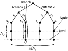
Fig. 1: SM tree-search decoder for $M=2$, $N_{t}=2$, and $N_{r}=3$ with four branches.

III Minimum-Distance of Maximum-Length Algorithm

Unlike the existent SD algorithms in the literature, the proposed m-M algorithm performs only one node expansion at a time; the expanded node is chosen to be of minimum ED across all branches. The proposed algorithm jumps from one branch to another according to where the minimum ED is, and stops if the minimum ED occurs at the end of a fully expanded branch (i.e., maximum length).

For mathematical formulation, assume that $\mathbf{v}=\left[v_{1}\ldots v_{MN_{t}}\right]\in\mathbb{R}^{1\times MN_{t}}$ denote the vector of visited nodes, where $v_{j}$ takes integer values from $1$ up to $N_{r}$ and represents the number of nodes already visited of the $j$-th branch for $j=1,\ldots,MN_{t}$. Also, let $\mathbf{d}=\left[d_{v_{1},1}\ldots d_{v_{MN_{t}},MN_{t}}\right]\in\mathbb{R}^{1\times MN_{t}}$ denote the ED vector, where $d_{v_{j},j}$ is given by (4) by setting $i=v_{j}$ (i.e., $d_{v_{j},j}=\sum_{n=1}^{v_{j}}\left|y_{n}-x_{n,j}\right|^{2}$, where $d_{v_{j},j}$ represents the ED (node metric) of the $v_{j}$-th level for the $j$-th branch).

Algorithm 1 summarizes the proposed m-M algorithm that is explained as follows:

Step 1: Initialize all elements of $\mathbf{v}$ to unity (i.e., $v_{j}=1\,\,\forall j$), and then calculate each element of the vector $\mathbf{d}$ from (4) accordingly. It should be noted that the elements of $\mathbf{d}$ in this step represent the first ED of all branches (i.e., $\mathbf{d}=[d_{1,1}\ldots d_{1,MN_{t}}]$).

Step 2: Determine the argument of the minimum element of $\mathbf{d}$ as

$$j_{\text{min}}=\underset{j=1,\ldots,MN_{t}}{\text{arg}\,\text{min}}\{d_{v_{j},j}\}.$$ (7)

Step 3: Increase the $j_{\text{min}}$-th element of $\mathbf{v}$ by one

$$v_{j_{\text{min}}}\rightarrow v_{j_{\text{min}}}+1.$$ (8)

Note that this step ensures that the algorithm makes a single expansion to the minimum ED, which leads to the increase of the corresponding element of the vector $\mathbf{v}$ by one. The maximum value of $v_{j}\,\,\forall j$ that can be reached is $N_{r}$; therefore, we can define $\mathbf{j}_{\text{max}}$ as the set of indices whose values reached $N_{r}$, as

$$\mathbf{j}_{\text{max}}=\text{find}\left(\mathbf{v}=N_{r}\right),$$ (9)

where $\text{find}\left(\mathbf{v}=N_{r}\right)$ returns the indices of the elements of $\mathbf{v}$ that are equal to $N_{r}$. At the beginning, $\mathbf{j}_{\text{max}}$ is buffered as an empty set, and is updated when at least one branch is fully expanded.

Step 4: Update the $j_{\text{min}}$-th element of $\mathbf{d}$ by calculating the new $d_{v_{j_{\text{min}}},j_{\text{min}}}$ from (4) based on $v_{j_{\text{min}}}$ calculated from Step 3.

Step 5: Find the new $j_{\text{min}}$ from (7) as in Step 2, and then check whether the following condition is true or not:

$$j_{\text{min}}\in\mathbf{j}_{\text{max}}.$$ (10)

If $j_{\text{min}}\notin\mathbf{j}_{\text{max}}$, then go back to Step 2. Otherwise, find the index of the estimated transmitted combination as

$$\hat{j}_{\text{m-M}}=\underset{j\in\mathbf{j}_{\text{max}}}{\text{arg}\,\text{min}}\{d_{v_{j},j}\},$$ (11)

where $\hat{j}_{\text{m-M}}$ denotes the index of the estimated transmitted combination from the m-M algorithm. Note that in case of $v_{j}=N_{r}\,\,\forall j$ in (11), the ML version in (5) is obtained. The estimated transmitted combination from m-M algorithm, $\hat{\mathbf{x}}_{\text{m-M}}$, is

$$\hat{\mathbf{x}}_{\text{m-M}}=\mathbf{x}_{\hat{j}_{\text{m-M}}}.$$ (12)

Note that the condition in (10) is called the optimality condition, and guarantees that the ML solution will not be missed before stopping the m-M algorithm (i.e., $\hat{\mathbf{x}}_{\text{m-M}}=\hat{\mathbf{x}}_{\text{ML}}$).

• Initialize $\mathbf{v}=\left[1\,\,1\,\ldots\,1\right]\in\mathbb{R}^{1\times MN_{t}}$, $j_{\text{max}}=0$.

• Compute the elements of $\mathbf{d}=[d_{1,1}\ldots d_{1,MN_{t}}]$, where $d_{1,j}=\left|y_{1}-x_{1,j}\right|^{2}$ and $j=1,\ldots,MN_{t}$.

• Reserve an empty vector $\mathbf{j}_{\text{max}}=[.]$ as a buffer.

1: $\text{{while}}\,\,\,n\leq N_{r}MN_{t}$  do

2:    Find the index $j_{\text{min}}=\underset{j=1,\ldots,MN_{t}}{\text{arg}\,\text{min}}\{d_{v_{j},j}\}$.

3:    if $\mathbf{j}_{\text{max}}$ is NOT empty

4:      if $j_{\text{min}}\in\mathbf{j}_{\text{max}}$

5:         go to line 14.

6:      else

7:         go to line 10.

8:      end if

9:    end if

10:    Set $v_{j_{\text{min}}}\rightarrow v_{j_{\text{min}}}+1$, then Update $\mathbf{v}$.

11:    Update the $j_{\text{min}}$-th element of $\mathbf{d}$ as:

$d_{v_{j_{\text{min}}},j_{\text{min}}}\rightarrow d_{v_{j_{\text{min}}},j_{\text{min}}}+\left|y_{v_{j_{\text{min}}}}-x_{v_{j_{\text{min}}},j_{\text{min}}}\right|^{2}$.

12:    Update $\mathbf{j}_{\text{max}}$ based on $\mathbf{j}_{\text{max}}=\text{find}\left(\mathbf{v}=N_{r}\right)$.

13:    Set $n\rightarrow n+1$.

14: end while

• Estimate $\hat{\mathbf{x}}_{\text{m-M}}$ from $\hat{\mathbf{x}}_{\text{m-M}}=\mathbf{x}_{j_{\text{min}}}$.

Algorithm 1 Pseudo-code of the proposed m-M algorithm.

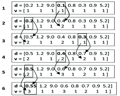
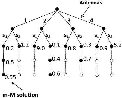
Fig. 2: A numerical example for the m-M algorithm ($3\times 4$ MIMO-SM system and $M=2$).

Fig. 2 illustrates a numerical example for the proposed m-M algorithm. Consider a $3\times 4$ MIMO system with $M=2$. Thus, we have $8$ branches with $3$ nodes/levels length. First, the m-M algorithm initializes $\mathbf{v}$ by all-ones, and calculates the the first ED of each branch. The m-M algorithm finds the minimum ED of $\mathbf{d}$, which is $0.1$ in our example. This ED corresponds to the $4$-th branch ($j_{\text{min}}=4$); thus, the m-M algorithm expands this node after increasing the $4$-th element of $\mathbf{v}$ by one (i.e., $v_{j_{\text{min}}}=v_{4}=2$ and $d_{2,4}=0.4$). In the second iteration, the m-M algorithm finds the new minimum ED in $\mathbf{d}$ (i.e., 0.2), which is placed in the first branch ($j_{\text{min}}=1$). Then, the first element of $\mathbf{v}$ is updated to be $2$ and the first element of $\mathbf{d}$ is updated accordingly (i.e., $v_{1}=2$ and $d_{2,1}=0.5$). The algorithm jumps from one branch to another according to the location of the minimum ED across all branches, as illustrated in iterations 3, 4, and 5. Note that the m-M algorithm detects one element of $\mathbf{v}$ reaches $N_{r}$ (i.e., full expansion for that branch) from iteration 5, which is the $4$-th branch. According to (10), the algorithm has to check if the new minimum ED comes at a fully expanded branch or not before deciding to stop. In our example, the algorithm will not stop at iteration 5 because there is a minimum ED at the first branch (i.e., 0.5). Therefore, the algorithm makes a single expansion to the first branch after updating the first element of $\mathbf{v}$ (i.e., $v_{1}=3$ and $d_{3,1}=0.55$); and then, it checks the place of the minimum ED once more. In this example, the iteration 6 shows that the minimum ED (i.e., 0.55) comes at the end of a fully expanded branch, which corresponds to the first branch (i.e., $\hat{j}_{\text{m-M}}=1$). Thus, the m-M algorithm stops and declares that the estimated transmitted combination is the first one (i.e., the first symbol was transmitted from the first antenna).

IV Complexity Analysis

In this paper, we consider the number of visited nodes inside the tree-search as the complexity indicator. Since $\mathbf{v}$ represents the visited nodes for each branch, the summation of its elements at the final iteration gives the total complexity of the m-M algorithm in terms of the number of visited nodes. Consider the complexity of the m-M algorithm denoted by $C_{\text{m-M}}=\text{sum}\left\{\mathbf{v}^{\text{f}}\right\}$, where $\mathbf{v}^{\text{f}}$ is the vector $\mathbf{v}$ at the final iteration. Since the elements of $\mathbf{v}^{\text{f}}$ are random variables (r.v.’s), $C_{\text{m-M}}$ is an r.v. as well. In this section, we provide a tight expression for the expected complexity of the proposed m-M algorithm in the case of perfect CSIR, as well as imperfect CSIR.

The average complexity of the m-M algorithm $C_{\text{m-M}}$ can be expressed as

$$C_{\text{m-M}}=\mathbb{E}\left\{\text{sum}\left\{\mathbf{v}^{\text{f}}\right\}\right\}.$$ (13)

Although the m-M algorithm is a breadth-first search algorithm, its expected complexity is equivalent to that of a depth-first SD algorithm with pruned radius, $R_{\text{m-M}}$, equal to the minimum ED of vector $\mathbf{d}$ at the final iteration (i.e., $0.55$ in the example illustrated in Fig. 2). Therefore, $R_{\text{m-M}}$ can be written as

$$R_{\text{m-M}}=d_{N_{r},\hat{j}_{\text{m-M}}}=\sum_{n=1}^{N_{r}}\left|y_{n}-x_{n,\hat{j}_{\text{m-M}}}\right|^{2}=\left\|\mathbf{y}-\hat{\mathbf{x}}_{\text{m-M}}\right\|^{2},$$ (14)

where $\hat{j}_{\text{m-M}}$ given from (11) and $\hat{\mathbf{x}}_{\text{m-M}}$ are given in (7) and (12), respectively. For simplicity, we consider $\hat{\mathbf{x}}_{\text{m-M}}\rightarrow\mathbf{x}_{t}$; this assumption most likely holds particularly in high signal-to-noise ratio (SNR) ($\hat{\mathbf{x}}_{\text{m-M}}=\hat{\mathbf{x}}_{\text{ML}}$ since the m-M algorithm guarantees the ML solution). Thus, substituting (2) and this assumption in (14) yields

$$R_{\text{m-M}}=\left\|\mathbf{w}\right\|^{2}.$$ (15)

It should be noted that the pruned radius in (14) is considered the optimum threshold that can be used in the SD-based algorithms. Since the decoding complexity of the proposed m-M algorithm is equivalent to that of a depth-first algorithm using the optimum pruned radius in (14), the proposed algorithm provides a better complexity than the optimum BER algorithms in the literature.

Now, we can write $C_{\text{m-M}}$ in (13) as [References], [References]

$$C_{\text{m-M}}\approx MN_{t}+\sum_{j=1}^{MN_{t}}\sum_{i=1}^{N_{r}}\mathbb{P}\text{r}\left(d_{i,j}\leq R_{\text{m-M}}\left|\mathbf{x}_{t},\mathbf{H},\sigma_{n}^{2},R_{\text{m-M}}\right.\right).$$ (16)

It is worth noting that (16) is the generic form of the expected complexity, and its closed-form solution depends on the algorithm itself. Note that (16) finds the probability of $d_{i,j}$ being visited when the SD radius is $R_{\text{m-M}}$ (the node is considered to be visited if $d_{i,j}\leq R_{\text{m-M}}$ and vice versa). Ideally, $\mathbb{P}\text{r}\left(d_{i,j}\leq R_{\text{m-M}}\right)$ under the conditions previously given should be zero or one. The correction factor $MN_{t}$ in (16) is needed since the $\mathbb{P}\text{r}\left(d_{i,j}\leq R_{\text{m-M}}\right)$ misses almost $MN_{t}$ nodes at the final iteration.

IV-A Perfect Channel State Information at the Receiver

To find the closed form expression of the right-hand-side of (16), the conditional probability distribution of $d_{i,j}$ should be determined first. From (2) and (4), we can rewrite (4) in terms of the real and imaginary components as

$d_{i,j}=\sum_{n=1}^{i}\left|\left(w_{n}^{\Re}+x_{n,t}^{\Re}-x_{n,j}^{\Re}\right)+\jmath\left(w_{n}^{\Im}+x_{n,t}^{\Im}-x_{n,j}^{\Im}\right)\right|^{2}$

$$=\sum_{n=1}^{i}\left(\mathcal{R}_{n}^{2}+\mathcal{I}_{n}^{2}\right),\hskip 28.45274pt$$ (17)

where $\mathcal{R}_{n}=w_{n}^{\Re}+x_{n,t}^{\Re}-x_{n,j}^{\Re}$ and $\mathcal{I}_{n}=w_{n}^{\Im}+x_{n,t}^{\Im}-x_{n,j}^{\Im}$ are Gaussian distributed with variances $\sigma_{n}^{2}/2$, and means $\left(x_{n,t}^{\Re}-x_{n,j}^{\Re}\right)$ and $\left(x_{n,t}^{\Im}-x_{n,j}^{\Im}\right)$, respectively. Consequently, $d_{i,j}$ is a non-central chi-squared r.v. with $2i$ degrees of freedom and non-centrality parameter $\gamma_{i,j}^{2}$ given by [References, (Ch. 2)]

$$\gamma_{i,j}^{2}=\sum_{n=1}^{i}\left[\left(x_{n,t}^{\Re}-x_{n,j}^{\Re}\right)^{2}+\left(x_{n,t}^{\Im}-x_{n,j}^{\Im}\right)^{2}\right].$$ (18)

The probability distribution function (pdf) of $d_{i,j}$ for $d_{i,j}\geq 0$ is calculated as [References, (Ch. 2)]

$f_{d_{i,j}}(d_{i,j})=\frac{1}{\sigma_{n}^{2}}\left(\frac{d_{i,j}}{\gamma_{i,j}^{2}}\right)^{(i-1)/2}$

$$\times\,\text{exp}\left(-\frac{\gamma_{i,j}^{2}+d_{i,j}}{\sigma_{n}^{2}}\right)\,I_{i-1}\left(\frac{\sqrt{d_{i,j}\,\gamma_{i,j}^{2}}}{\sigma_{n}^{2}/2}\right),$$ (19)

where $I_{i-1}\left(\centerdot\right)$ is the first kind modified Bessel function of order $(i-1)$. Since $d_{i,j}$ has an even degrees of freedom, the closed form expression of the cumulative distribution function (cdf) for (19) is given as [References, (Ch. 2)]

$\mathbb{P}\text{r}\left(d_{i,j}\leq R_{\text{m-M}}\left|\mathbf{x}_{t},\mathbf{H},\sigma_{n}^{2},R_{\text{m-M}}\right.\right)=$

$$\hskip 99.58464pt1-Q_{i}\left(\frac{\gamma_{i,j}}{\sigma_{n}/\sqrt{2}}\,,\,\frac{\sqrt{R_{\text{m-M}}}}{\sigma_{n}/\sqrt{2}}\right),$$ (20)

where $Q_{i}(\centerdot,\centerdot)$ denotes the generalized Marcum function of order $i$.

To remove the dependency of (20) on the instantaneous value of $R_{\text{m-M}}$, an expectation over the pdf of $R_{\text{m-M}}$ should be calculated. (15) can be written in terms of its real and imaginary components as

$$R_{\text{m-M}}=\sum_{n=1}^{N_{r}}\left[\left(w_{n}^{\Re}\right)^{2}+\left(w_{n}^{\Im}\right)^{2}\right].$$ (21)

Therefore, $R_{\text{m-M}}$ is a central chi-square r.v. with $2N_{r}$ degrees of freedom and its pdf, $f_{R_{\text{m-M}}}(R_{\text{m-M}})$, is [References, (Ch. 2)]

$$f_{R_{\text{m-M}}}(R_{\text{m-M}})=\frac{\left(R_{\text{m-M}}\right)^{N_{r}-1}}{\sigma_{n}^{2N_{r}}\left(N_{r}-1\right)!}\,\text{exp}\left(\frac{-R_{\text{m-M}}}{\sigma_{n}^{2}}\right).$$ (22)

From (20) and (22), the expected value of (20) over the pdf of $R_{\text{m-M}}$ can be written as

$\mathbb{P}\text{r}\left(d_{i,j}\leq R_{\text{m-M}}\left|\mathbf{x}_{t},\mathbf{H},\sigma_{n}^{2}\right.\right)=$

$$\int_{0}^{\infty}\left[1-Q_{i}\left(\frac{\gamma_{i,j}}{\sigma_{n}/\sqrt{2}}\,,\,\frac{\sqrt{R_{\text{m-M}}}}{\sigma_{n}/\sqrt{2}}\right)\right]f_{R_{\text{m-M}}}(R_{\text{m-M}})\,\,\,\,\text{d}R_{\text{m-M}}.$$ (23)

The closed form solution of the integration in (23) can be found in [References], and then, the complexity in (16) is expressed as

$$\begin{gathered}C_{\text{m-M}}\approx MN_{t}+\sum_{j=1}^{MN_{t}}\sum_{i=1}^{N_{r}}\left[1-\left[1-\frac{\text{exp}\left(-\gamma_{i,j}^{2}/\sigma_{n}^{2}\right)}{2^{N_{r}}}\right.\right.\\ \times\left[\Phi_{1}\left(N_{r},1,1;\frac{1}{2},\frac{\gamma_{i,j}^{2}}{2\sigma_{n}^{2}}\right)\hskip 35.56593pt\right.\\ \left.\left.\left.\hskip 39.83385pt-\sum_{k=1}^{i-1}\frac{\left(N_{r}\right)_{k}}{2^{k}\,k!}\,_{1}F_{1}\left(N_{r}+k;k+1;\frac{\gamma_{i,j}^{2}}{2\sigma_{n}^{2}}\right)\right]\right]\right],\end{gathered}$$ (24)

where $\left(N_{r}\right)_{k}$ denotes the Pochhammer symbol, $\Phi_{1}$ is the Humbert hypergeometric function of the first kind, and ${}_{1}F_{1}$ denotes the Kummer hypergeometric function [References].

IV-B Imperfect Channel State Information at the Receiver

In this subsection, the complexity of the proposed m-M algorithm in (16) is assessed in the presence of imperfect CSIR. To the best of the authors’ knowledge, in case of imperfect CSIR, the expected complexity is not analyzed in the literature. Assume that there is an error between the estimated channel coefficient at the receiver side and the actual channel coefficient, which is denoted by $\mathbf{e}\sim\mathcal{C}\mathcal{N}\left(0,\sigma_{e}^{2}\right)$, where $\sigma_{e}^{2}$ is the variance of the error in the channel estimation. Thus, the estimated channel entry becomes $\hat{\mathbf{h}}=\mathbf{h}+\mathbf{e}$ and the combination element in (4) becomes $x_{n,j}+\hat{e}_{n,j}$, where $\hat{e}_{n,j}=e_{n}s_{j}$, with $s_{j}$ as the QAM symbol in $j$-th combination with energy of $\left|s_{j}\right|^{2}$ and $e_{n}$ as the $n$-th element of vector $\mathbf{e}$. In this case, for least square solution of (4), $\hat{\mathbf{h}}\sim\mathcal{C}\mathcal{N}\left(0,1+\sigma_{e}^{2}\right)$ depends on $\mathbf{h}$ with a correlation coefficient of $\rho=1/\sqrt{1+\sigma_{e}^{2}}$ [References]-[References], [References, (p. 282)]; the conditional variance of the elements of the noisy received vector, $\zeta_{j}^{2}$, is given by [References], [References]

$$\zeta_{j}^{2}=\text{Var}\left(y|\hat{\mathbf{h}}\right)=\sigma_{n}^{2}+\left(1-\rho^{2}\right)\left|s_{j}\right|^{2}.$$ (25)

It should be noted that the $\sigma_{e}^{2}$ may be considered as fixed or variable when SNR changes. In theory, the error in channel estimation decreases as the SNR increases [References], [References]; therefore, we can consider $\sigma_{e}^{2}=1/\text{snr}$ in case of variable $\sigma_{e}^{2}$ where snr denotes the signal-to-noise ratio in linear scale (i.e., SNR = $10\text{lo$g_{10}$}\left(\text{snr}\right)$).

$d_{i,j}$ in (17) in the case of imperfect-CSIR is denoted by $\hat{d}_{i,j}$ and given as

$\hat{d}_{i,j}=\sum_{n=1}^{i}\left|\left(w_{n}^{\Re}-\hat{e}_{n,j}^{\Re}+x_{n,t}^{\Re}-x_{n,j}^{\Re}\right)\right.$

$$\left.+\jmath\left(w_{n}^{\Im}-\hat{e}_{n,j}^{\Im}+x_{n,t}^{\Im}-x_{n,j}^{\Im}\right)\right|^{2}=\sum_{n=1}^{i}\left(\mathcal{\hat{R}}_{n}^{2}+\hat{\mathcal{I}}_{n}^{2}\right),$$ (26)

where $\mathcal{\hat{R}}_{n}=w_{n}^{\Re}-\hat{e}_{n,j}^{\Re}+x_{n,t}^{\Re}-x_{n,j}^{\Re}$ and $\hat{\mathcal{I}}_{n}=w_{n}^{\Im}-\hat{e}_{n,j}^{\Im}+x_{n,t}^{\Im}-x_{n,j}^{\Im}$ are Gaussian distributed with variances $\zeta_{j}^{2}/2$, and means $\left(x_{n,t}^{\Re}-x_{n,j}^{\Re}\right)$ and $\left(x_{n,t}^{\Im}-x_{n,j}^{\Im}\right)$, respectively. Consequently, $\hat{d}_{i,j}$ is a non-central chi-squared r.v. with $2i$ degrees of freedom and non-centrality parameter $\gamma_{i,j}^{2}$ given by (18), and its pdf for $\hat{d}_{i,j}\geq 0$ becomes [References, (Ch. 2)]

$f_{\hat{d}_{i,j}}(\hat{d}_{i,j})=\frac{1}{\zeta_{j}^{2}}\left(\frac{\hat{d}_{i,j}}{\gamma_{i,j}^{2}}\right)^{(i-1)/2}$

$$\times\,\text{exp}\left(-\frac{\gamma_{i,j}^{2}+\hat{d}_{i,j}}{\zeta_{j}^{2}}\right)\,I_{i-1}\left(\frac{\sqrt{\hat{d}_{i,j}\,\gamma_{i,j}^{2}}}{\zeta_{j}^{2}/2}\right).$$ (27)

Therefore, (20) becomes

$\mathbb{P}\text{r}\left(\hat{d}_{i,j}\leq\hat{R}_{\text{m-M}}\left|\mathbf{x}_{t},\mathbf{H},\sigma_{n}^{2},\sigma_{e}^{2},\hat{R}_{\text{m-M}}\right.\right)=$

$$\hskip 99.58464pt1-Q_{i}\left(\frac{\gamma_{i,j}}{\zeta_{j}/\sqrt{2}}\,,\,\frac{\sqrt{\hat{R}_{\text{m-M}}}}{\zeta_{j}/\sqrt{2}}\right),$$ (28)

where $\hat{R}_{\text{m-M}}$ denotes the threshold of the m-M algorithm in the case of imperfect CSIR. It should be noted that for the case of imperfect CSIR, the threshold in (21) becomes

$$\hat{R}_{\text{m-M}}=\sum_{n=1}^{N_{r}}\left[\left(w_{n}^{\Re}-\hat{e}_{n,t}^{\Re}\right)^{2}+\left(w_{n}^{\Im}-\hat{e}_{n,t}^{\Im}\right)^{2}\right],$$ (29)

where $\left(w_{n}^{\Re}-\hat{e}_{n,t}^{\Re}\right)$ and $\left(w_{n}^{\Im}-\hat{e}_{n,t}^{\Im}\right)$ are Gaussian distributed with zero-mean and variance of $\zeta_{t}^{2}/2$, where

$$\zeta_{t}^{2}=\sigma_{n}^{2}+\left(1-\rho^{2}\right)\left|s_{t}\right|^{2},$$ (30)

with $s_{t}$ as the transmitted QAM symbol with energy $\left|s_{t}\right|^{2}$.

Consequently, $\hat{R}_{\text{m-M}}\geq 0$ is a central chi-squared distributed r.v. with $2N_{r}$ degrees of freedom and its pdf is given by [References, (Ch. 2)]

$$f_{\hat{R}_{\text{m-M}}}(\hat{R}_{\text{m-M}})=\frac{\left(\hat{R}_{\text{m-M}}\right)^{N_{r}-1}}{\zeta_{t}^{2N_{r}}\left(N_{r}-1\right)!}\hskip 4.2679pt\text{exp}\left(\frac{-\hat{R}_{\text{m-M}}}{\zeta_{t}^{2}}\right).$$ (31)

From (28) and (31), the expected value of (28) over the pdf of $\hat{R}_{\text{m-M}}$ can be written as

$\mathbb{P}\text{r}\left(\hat{d}_{i,j}\leq\hat{R}_{\text{m-M}}\left|\mathbf{x}_{t},\mathbf{H},\sigma_{n}^{2},\sigma_{e}^{2}\right.\right)=$

$$\int_{0}^{\infty}\left[1-Q_{i}\left(\frac{\gamma_{i,j}}{\zeta_{j}/\sqrt{2}}\,,\,\frac{\sqrt{\hat{R}_{\text{m-M}}}}{\zeta_{j}/\sqrt{2}}\right)\right]f_{\hat{R}_{\text{m-M}}}(\hat{R}_{\text{m-M}})\,\,\,\,\text{d}\hat{R}_{\text{m-M}}.$$ (32)

The closed form of the integration in (32) can be found in [References], and then, the complexity in (16) is obtained as

$$\begin{gathered}\hat{C}_{\text{m-M}}\approx MN_{t}+\sum_{j=1}^{MN_{t}}\sum_{i=1}^{N_{r}}\left[1-\left[1-\frac{\zeta_{j}^{2N_{r}}\,\text{exp}\left(-\gamma_{i,j}^{2}/\zeta_{j}^{2}\right)}{\left(\zeta_{j}^{2}+\zeta_{t}^{2}\right)^{N_{r}}}\right.\right.\\ \times\left[\Phi_{1}\left(N_{r},1,1;\frac{\zeta_{t}^{2}}{\zeta_{j}^{2}+\zeta_{t}^{2}},\frac{\gamma_{i,j}^{2}\,\zeta_{t}^{2}}{\zeta_{j}^{2}\left(\zeta_{j}^{2}+\zeta_{t}^{2}\right)}\right)\hskip 35.56593pt\right.\\ \left.\left.\left.\hskip 14.22636pt-\sum_{k=1}^{i-1}\frac{\left(N_{r}\right)_{k}}{k!}\,_{1}F_{1}\left(N_{r}+k;k+1;\frac{\gamma_{i,j}^{2}\,\zeta_{t}^{2}}{\zeta_{j}^{2}\left(\zeta_{j}^{2}+\zeta_{t}^{2}\right)}\right)\right]\right]\right].\end{gathered}$$ (33)

V Optimality of BER Performance

In this section, we discuss the BER performance optimality of the proposed m-M algorithm based on the condition in (10). The effect of omitting this condition on the proposed m-M algorithm is also studied. We define an indicator for the BER performance optimality as the number of times the proposed m-M algorithm misses the ML solution, referred to as the number of misses (NoM). In other words, the BER of the m-M algorithm will be the same as the ML BER if the NoM equals zero and vice versa. It should be noted that NoM is an r.v. that depends on the SNR and $\sigma_{e}^{2}$.

Let us invoke the general expression of the union bound error probability of SM-ML detector as [References], [References]

$$P_{b}=\frac{1}{\left(\eta\right)2^{\eta}}\sum_{k=1}^{2^{\eta}}\sum_{l=1}^{2^{\eta}}\delta_{k,l}\mathcal{\mathbb{E}}\left\{\mathbb{P}\text{r}^{\left(\text{ML}\right)}\left(\mathbf{x}_{k}\rightarrow\tilde{\mathbf{x}}_{l}\right)\right\},$$ (34)

where $P_{b}$ is the union bound probability, $\mathbb{P}\text{r}^{\left(\text{ML}\right)}\left(\mathbf{x}_{k}\rightarrow\tilde{\mathbf{x}}_{l}\right)$ stands for the pairwise error probability (PEP) of the proposed SM-ML decoder, $\delta_{k,l}$ represents the number of bit errors which corresponds to the instant PEP event, and the spectral efficiency $\eta$ is given from (1). Let us consider that $\Delta^{\text{m-M}}$ is the NoM between the m-M algorithm solution and the ML solution. Now, the PEP of the m-M algorithm is denoted by $\mathbb{P}\text{r}^{\left(\text{m-M}\right)}\left(\mathbf{x}_{k}\rightarrow\tilde{\mathbf{x}}_{l}\right)$ and given as [References]

$$\mathbb{P}\text{r}^{\left(\text{m-M}\right)}\left(\mathbf{x}_{k}\rightarrow\tilde{\mathbf{x}}_{l}\right)=\mathbb{P}\text{r}^{\left(\text{ML}\right)}\left(\mathbf{x}_{k}\rightarrow\tilde{\mathbf{x}}_{l}\right)+\mathbb{P}\text{r}\left(\Delta^{\text{m-M}}\neq 0\right).$$ (35)

According to (10), if the m-M algorithm detects a minimum ED at the end of fully expanded branch, this means that no further expansion will happen in the current minimum ED (the branch length can not be $N_{r}+1$) and the current minimum ED is a global minimum across all other branches. Therefore, the ML solution will not be missed (i.e., $\mathbb{P}\text{r}\left(\Delta^{\text{m-M}}\neq 0\right)=0$) and the union bound error probability of the proposed m-M algorithm is exactly the same as (34).

To study the effect of removing the optimality condition in (10), consider an m-M algorithm without this condition, referred to as the m-Mw algorithm. It should be noted that the m-Mw algorithm is not a stand-alone algorithm, and it is mentioned here to discuss the optimality condition in (10) for the proposed m-M algorithm. The m-Mw algorithm stops and declares the solution whenever only one branch is fully expanded. In such a case, the NoM takes a non-zero value and $\mathbb{P}\text{r}\left(\Delta^{\text{m-Mw}}\neq 0\right)\neq 0$. Fig. 3 shows the average NoM versus SNR; $10^{4}$ Rayleigh flat fading channel realizations are run for each SNR value, for $8\times 8$ MIMO-SM using 8-QAM. As we can see, the NoM reduces as SNR increases and $\sigma_{e}^{2}$ decreases. For instance, the m-Mw algorithm misses $2020$, $564$ and $20$ ML solution out of $10^{4}$ runs at SNR of $0$, $5$ and $10$ dB, respectively, in case of perfect CSIR; for imperfect CSIR with $\sigma_{e}^{2}=0.2$, the NoM for the m-Mw algorithm is $2371$, $1188$ and $420$ out of $10^{4}$ runs at SNR of $0$, $5$ and $10$ dB, respectively.

Hence, the condition in (10) ensures that the minimum ED which comes at the end of a fully expanded branch is a global minimum across all branches; thus, the ML solution is achieved. Additionally, omitting the condition in (10) leads to a significant BER deterioration when compared with the ML performance.

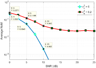
Fig. 3: Average number of NoM of the m-Mw algorithm for $8\times 8$ MIMO-SM and $8$-QAM.

VI Numerical Results and Discussions

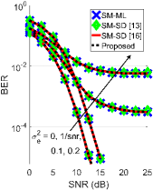
(a) 8-QAM for $8\times 8$ MIMO-SM.

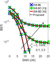
(b) 16-QAM for $16\times 16$ MIMO-SM.

Fig. 4: BER comparison of determined MIMO-SM system for different decoders.

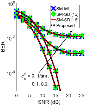
(a) 8-QAM for $6\times 8$ MIMO-SM.

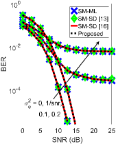
(b) 16-QAM for $12\times 16$ MIMO-SM.

Fig. 5: BER comparison of under-determined MIMO-SM system for different decoders.

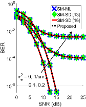
(a) 8-QAM for $10\times 8$ MIMO-SM.

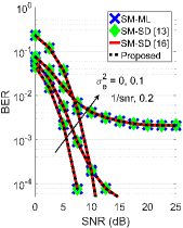
(b) 16-QAM for $20\times 16$ MIMO-SM.

Fig. 6: BER comparison of over-determined MIMO-SM system for different decoders.

In this section, we evaluate the behavior of the proposed m-M algorithm in terms of BER and decoding complexity. In addition, comparisons between the m-M algorithm and SM-SD algorithms in the literature are presented. Since the m-M algorithm provides the optimal BER performance, we consider the SM-SD algorithms (such as given in [References] and [References]) in comparisons. Three scenarios are considered: a) perfect CSIR ($\sigma_{e}^{2}=0$), b) imperfect CSIR with fixed $\sigma_{e}^{2}$ ($\sigma_{e}^{2}=0.1$ and $0.2$), and c) imperfect CSIR with variable $\sigma_{e}^{2}$ ($\sigma_{e}^{2}=1/\text{snr}$). Two spectral efficiency values are considered: $\eta=6$ bpcu using 8-QAM for $N_{r}\times 8$ MIMO-SM system, and $\eta=8$ bpcu using 16-QAM for $N_{r}\times 16$ MIMO-SM system. The value of $N_{r}$ for both cases describes the type of the system. In the case of determined MIMO-SM system, $N_{r}=N_{t}$ (i.e., $N_{r}=8$ and $16$ for $\eta=6$ and 8, respectively). For under-determined MIMO-SM system, $N_{r}<N_{t}$ (e.g., $N_{r}=6$ and $12$ for $\eta=6$ and $8$, respectively). Finally, we have an over-determined MIMO-SM system if $N_{r}>N_{t}$ (e.g., $N_{r}=10$ and $20$ for $\eta=6$ and $8$, respectively). Monte Carlo simulations are used to obtain the presented results for all scenarios by running at least $5\times 10^{5}$ Rayleigh flat fading channel realizations.

VI-A BER Comparison

In this subsection, the BER performance of the SM-ML, SM-SD [References], SM-SD [References], and proposed m-M algorithms are compared with respect to SNR. Figs. 4, 5 and 6 show the BER performance of different SM decoders for determined, under-determined, and over-determined MIMO-SM systems, respectively. The left sub-plots in all three figures present $\eta=6$ bpcu, while the right ones show $\eta=8$ bpcu. As observed from these figures, the two SM-SD algorithms in [References] and [References], as well as the proposed m-M algorithm provide the same SM-ML BER for all values of $\sigma_{e}^{2}$ (i.e., 0, 0.1, 0.2, and 1/snr). As expected, the best BER is obtained when $\sigma_{e}^{2}=0$, while the BER degrades for increasing values of $\sigma_{e}^{2}$. Unlike the BER obtained from having $\sigma_{e}^{2}=1/\text{snr}$, an error floor occurs in the case of $\sigma_{e}^{2}=0.1$ and 0.2 even in high SNR due to the fixed values of $\sigma_{e}^{2}$. The error floor is mitigated as $N_{r}$ increases. For instance, the error floor of the $\sigma_{e}^{2}=0.1$ curve in Fig. 5(b) can not be reduced to $5\times 10^{-4}$ when $N_{r}=12$; when $N_{r}=16$ in Fig. 4(b) for the $\sigma_{e}^{2}=0.1$ curve, the error floor occurs at $10^{-4}$; however, it further reduces to $10^{-5}$ when $N_{r}=20$ in Fig. 6(b) for the $\sigma_{e}^{2}=0.1$ curve.

It can be seen from these figures that there is no preference in BER between the proposed m-M algorithm and the other SM-SD algorithms in [References] and [References]. For all presented scenarios, the low-complexity algorithms (the m-M algorithm, and SM-SD algorithms in [References] and [References]) provide the same BER as the SM-ML detection. It is worth noting that in practice, the channel estimation accuracy improves as the SNR increases (i.e., $\sigma_{e}^{2}=1/\mathrm{snr}$), and the ML BER performance can be still reasonable, as seen from Figs. 4, 5 and 6.

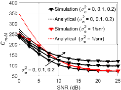
(a) 8-QAM for $8\times 8$ MIMO-SM.

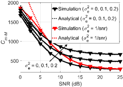
(b) 16-QAM for $16\times 16$ MIMO-SM.

Fig. 7: Complexity of determined MIMO-SM system for the proposed m-M algorithm.

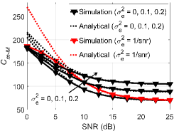
(a) 8-QAM for $6\times 8$ MIMO-SM.

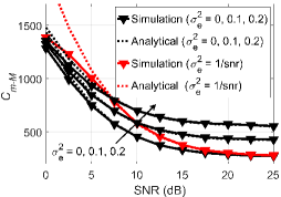
(b) 16-QAM for $12\times 16$ MIMO-SM.

Fig. 8: Complexity of under-determined MIMO-SM system for the proposed m-M algorithm.

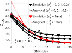
(a) 8-QAM for $10\times 8$ MIMO-SM.

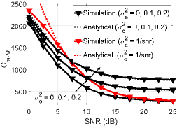
(b) 16-QAM for $20\times 16$ MIMO-SM.

Fig. 9: Complexity of over-determined MIMO-SM system for the proposed m-M algorithm.

VI-B Analytical Complexity Assessment

In this subsection, we evaluate the accuracy of the analytical expressions for the expected decoding complexity of the m-M algorithm given in (24) and (33). As mentioned before, the number of visited nodes (VNs) is used as a measure for the decoding complexity of all algorithms in this paper. Figs. 7, 8 and 9 present the comparison results between the analytical expressions and computer simulation results of the determined, under-determined and over-determined MIMO-SM systems, respectively, for $\eta=6$ and $8$ bpcu. In all figures, the analytical expression for $\sigma_{e}^{2}=0$ is given from (24), while the analytical expression for $\sigma_{e}^{2}=0.1$, $0.2$ and $\left(1/\text{snr}\right)$ is given from (33). From these figures, we observe that the analytical expressions in (24) and (33) match the computer simulation results after SNR values of 5 dB, while some mismatches occur at low SNR values.

It should be noted that the mismatch between the analytical expressions and simulation results at low SNR values comes from the assumptions of $\hat{\mathbf{x}}_{\text{m-M}}\rightarrow\mathbf{x}_{t}$ in (15). At low SNR, the ML solution (the same as $\hat{\mathbf{x}}_{\text{m-M}}$) misses the true solution, $\mathbf{x}_{t}$, which means that $\left\|\mathbf{y}-\mathbf{x}_{t}\right\|_{F}^{2}>\left\|\mathbf{y}-\hat{\mathbf{x}}_{\text{m-M}}\right\|_{F}^{2}$. In other words, the threshold $R_{\text{m-M}}$ in (15) used for the analytical expressions will be greater than the actual threshold in (14), which leads to the count of more nodes than the reality. By increasing the SNR, the ML solution most probably estimates the true solution; the assumption of $\hat{\mathbf{x}}_{\text{m-M}}\rightarrow\mathbf{x}_{t}$ becomes more reliable. In the case of $\sigma_{e}^{2}=1/\text{snr}$, $\sigma_{e}^{2}$ becomes very high at low SNR values (e.g., $\sigma_{e}^{2}=1$ at zero SNR) which dramatically affects the accuracy of (33).

As it can be seen from these figures, the derived analytical expressions in (24) and (33) accurately describe the decoding complexity of the proposed m-M algorithm in both perfect and imperfect CSIR especially at high SNR values for determined, under-determined, and over-determined MIMO-SM systems.

VI-C Complexity Comparison

In this subsection, we compare the complexity of the proposed m-M algorithm with the optimal BER performance SM-SD algorithms ([References] and [References]). It should be noted that the threshold of the SM-SD algorithm in [References] is optimized to provide the optimal BER. The comparison goal is to determine the decoding complexity reduction ratio between the desired and SM-ML algorithms, which is given as

$$C_{\text{R}}=\frac{MN_{t}N_{r}-C_{\Lambda}}{MN_{t}N_{r}}=1-\frac{C_{\Lambda}}{MN_{t}N_{r}},$$ (36)

where $C_{\text{R}}$ denotes the complexity reduction ratio, $MN_{t}N_{r}$ is the decoding complexity of the ML detector, and $C_{\Lambda}$ denotes the decoding complexity of the target algorithm with $\Lambda\in\left\{\text{m-M},\,\,\text{SM-SD}\,\text{[13]},\,\,\text{SM-SD}\,\text{[16]}\right\}$. The minimum number of nodes that can be visited by any algorithm is a one fully expanded branch (i.e., $N_{r}$ nodes) in addition to the nodes of the first row in the tree-search (i.e., $MN_{t}-1$ nodes). Thus, we can define the maximum reduction in the decoding complexity ratio that can be achieved by any algorithm, $C_{\text{R}}^{\text{max}}$, as

$$C_{\text{R}}^{\text{max}}=1-\frac{N_{r}+MN_{t}-1}{MN_{t}N_{r}}.$$ (37)

Figs. 10, 11 and 12 show the complexity reduction ratio in (36) versus different values of SNR for determined, under-determined, and over-determined MIMO-SM systems, respectively. Each figure contains four sub-figures which represent all scenarios of $\sigma_{e}^{2}$ (i.e., 0, 0.1, 0.2, and $1/$snr), while each sub-figure presents the two available spectral efficiencies, $\eta=6$ and $8$ bpcu. According to (37), $C_{\text{R}}^{\text{max}}=86.1\%$ and $93.4\%$ in Fig. 10 for $\eta=6$ and $8$ bpcu, respectively; $C_{\text{R}}^{\text{max}}=82\%$ and $91.3\%$ in Fig. 11 for $\eta=6$ and $8$ bpcu, respectively; and $C_{\text{R}}^{\text{max}}=88.6\%$ and $94.6\%$ in Fig. 12 for $\eta=6$ and $8$ bpcu, respectively.

In the case of $\sigma_{e}^{2}=0$ and $1/$snr, the proposed m-M algorithm provides the best reduction in the decoding complexity ratio over the SM-SD [References] and SM-SD [References] algorithms. The m-M algorithm as well as the other two algorithms reach to $C_{\text{R}}^{\text{max}}$ at high SNR. It should be noted that when $\eta$ increases, the decoding complexity ratio increases for all algorithms. In the case of fixed $\sigma_{e}^{2}$ (i.e., 0.1 and 0.2), no algorithm reaches $C_{\text{R}}^{\text{max}}$. However, the proposed m-M algorithm provides the best reduction in the decoding complexity ratio for all values of SNR. Also, as $\sigma_{e}^{2}$ increases, the reduction in complexity gain of the m-M algorithm over the other two algorithm increases.

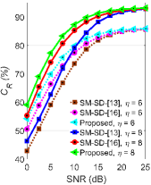
(a) $\sigma_{e}^{2}=0$.

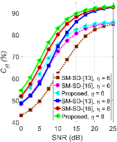
(b) $\sigma_{e}^{2}=1/\text{snr}$.

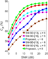
(c) $\sigma_{e}^{2}=0.1$.

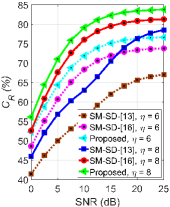
(d) $\sigma_{e}^{2}=0.2$.

Fig. 10: Complexity reduction comparison of determined MIMO-SM system for different decoders.

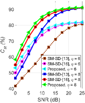
(a) $\sigma_{e}^{2}=0$.

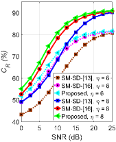
(b) $\sigma_{e}^{2}=1/\text{snr}$.

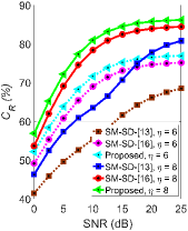
(c) $\sigma_{e}^{2}=0.1$.

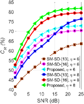
(d) $\sigma_{e}^{2}=0.2$.

Fig. 11: Complexity reduction comparison of under-determined MIMO-SM system for different decoders.

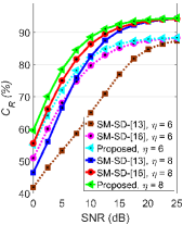
(a) $\sigma_{e}^{2}=0$.

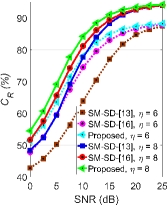
(b) $\sigma_{e}^{2}=1/\text{snr}$.

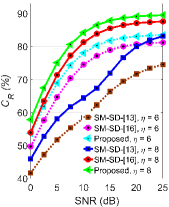
(c) $\sigma_{e}^{2}=0.1$.

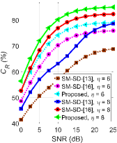
(d) $\sigma_{e}^{2}=0.2$.

Fig. 12: Complexity reduction comparison of over-determined MIMO-SM system for different decoders.

As it can be seen from these figures, the proposed m-M algorithm provides a better complexity reduction ratio in the low SNR in the case of perfect CSIR and variable $\sigma_{e}^{2}$. Moreover, it has the superiority over the existing SM-SD algorithms for all values of SNR in the case of imperfect CSIR with fixed $\sigma_{e}^{2}$. In addition, the m-M algorithm is more robust to the increase of $\sigma_{e}^{2}$ than the existing SM-SD algorithms.

VI-D Complexity Reduction Sensitivity

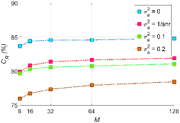
Fig. 13: Complexity reduction of the proposed m-M algorithm for $N_{t}=N_{r}=16$ and variable $M$.

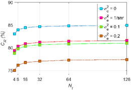
Fig. 14: Complexity reduction of the proposed m-M algorithm for $M=N_{r}=16$ and variable $N_{t}$.

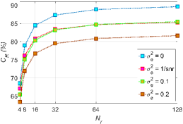
Fig. 15: Complexity reduction of the proposed m-M algorithm for $N_{t}=M=16$ and variable $N_{r}$.

We have noticed from Figs. 10, 11 and 12 that the reduction in the decoding complexity ratio for the m-M algorithm increases as the MIMO-SM dimensions ($M$, $N_{t}$, and $N_{r}$) increase. However, we need to determine which dimension affects more the complexity reduction ratio. In this subsection, we assess the reduction in the complexity ratio versus only one MIMO-SM dimension.

In Fig. 13, the decoding complexity reduction ratio of the m-M algorithm is assessed versus the QAM order, $M$, for the $16\times 16$ MIMO-SM system. It can be seen that the complexity reduction ratio slightly increases as $M$ increases. For example, for $\sigma_{e}^{2}=0.2$, the complexity reduction ratio increases from $76\%$ to $78.5\%$ at $M=8$ and $128$, respectively. Thus, the complexity reduction ratio of the proposed m-M algorithm is sensitive to the slightly change of $M$.

In Fig. 14, we evaluate the decoding complexity reduction ratio of the m-M algorithm versus $N_{t}$ at $N_{r}=M=16$. It can be noticed that the increase of the decoding complexity reduction is negligible in comparison with the case of variable $N_{t}$. Consequently, the change of $N_{t}$ has almost no effect on the decoding complexity ratio of the m-M algorithm.

The decoding complexity reduction is evaluated versus different values of $N_{r}$ in Fig. 15 for $N_{t}=M=16$. We can see from this figure that the complexity reduction ratio increases from $68\%$ at $N_{r}=4$ to $90\%$ at $N_{r}=128$ for $\sigma_{e}^{2}=0$, and from $64\%$ at $N_{r}=4$ to $82\%$ at $N_{r}=128$ for $\sigma_{e}^{2}=0.2$. Thus, the decoding complexity of the m-M algorithm increases logarithmically as $N_{r}$ increases.

Finally, we can see from these figures that the decoding complexity reduction ratio of the m-M algorithm is sensitive to the change of $N_{r}$, while is nonsensitive to the changes of $N_{t}$ or $M$.

VI-E Discussions

As seen from our comprehensive comparisons, the proposed m-M algorithm provides significant reduction in the decoding complexity basically without BER performance loss. For SM systems, compressive sensing (CS)-based algorithms have been recently proposed in [References]-[References] to provide sub-optimal BER performance with a reduction in the decoding complexity. These CS-based algorithms exploit the sparsity of the SM signals to provide low-complexity detection at the expense of BER deterioration. Normally, the CS-based algorithms are suitable for over-determined MIMO-SM systems (i.e., $N_{r}>N_{t}$) to reduce the BER performance gap versus the ML solution. The authors of [References] have proposed an enhanced Bayesian CS (EBCS) algorithm to provide low-complexity detection with near ML BER performance. The minimum decoding complexity of the EBCS algorithm in [References] can be achieved at high SNR, which is about $\mathcal{O}(N_{r}N_{t}^{2})+\mathcal{O}(N_{r}N_{t})+\mathcal{O}(N_{t})+\mathcal{O}(N_{r})$ floating point operations (flops). Since the ML decoder costs $9MN_{r}N_{t}$ flops, the maximum complexity reduction that can be achieved from [References] when compared with the ML decoder in high SNR is $87.2\%$ and $88.1\%$ for $12\times 8$ MIMO-SM with 8-QAM and $20\times 16$ MIMO-SM with 16-QAM, respectively. As shown in Fig. 12-(a) and (37), the proposed m-M algorithm provides $88.6\%$ and $94.6\%$ complexity reduction after 15 dB for $12\times 8$ MIMO-SM with 8-QAM and $20\times 16$ MIMO-SM with 16-QAM, respectively. Thus, the proposed algorithm has a higher complexity reduction without any BER performance loss when compared with the ML decoder.

Another recent low-complexity algorithm that provides a near-ML BER performance is proposed in [References] by dividing the tree-search into $N_{t}$ subtrees with $2N_{r}$ levels (for the real-form representation of (3)) and $M$ branches. The transmit and receive antennas are ordered to reach the solution faster. In the first subtree, the algorithm visits a different number of nodes in each level, $K=[k_{1}\,\,k_{2}\,\,\ldots k_{2N_{r}}]$, where $k_{i}$ represents the number of best nodes that should be kept in the $i$-th level and expanded in the next level. The minimum ED at the final level is used as a pruned radius for scanning the next $N_{t}-1$ subtrees by applying the SD concept in [References]. In high SNR, the minimum decoding complexity of the algorithm in [References] is $(\sum_{i=1}^{2N_{r}}k_{i})+M(N_{t}-1)$ visited nodes plus the cost of Eq. (5) in [References]. As discussed in (37), the proposed m-M algorithm can visit only $(2N_{r}+MN_{t}-1)$ nodes to achieve the optimum BER performance. For instance, for a $4\times 4$ MIMO-SM system with 64-QAM and $K=[64\,\,26\,\,26\,\,8\,\,8\,\,2\,\,2\,\,1]$ as mentioned in [References], the minimum decoding complexity of [References] in high SNR is $329$ visited nodes plus the cost of Eq. (5) in [References], while our proposed algorithm visits only 263 nodes to achieve the optimum BER performance in high SNR (almost high SNR is after 15 dB, as shown in Figs. 10, 11 and 12). Thus, the m-M algorithm provides a lower decoding complexity than the algorithm in [References] without losing the optimality of BER performance.

For high rate SM transmissions, one of the suggested solutions is to use a high value of $N_{t}$. Two systems are proposed to provide high rate transmission using smaller $N_{t}$; 1) generalized SM (GSM) which activates more than one transmit antenna at a time [References], and 2) quadrature SM (QSM) which delivers the symbols using the in-phase and quadrature dimensions [References]. At the receiver side, the GSM and QSM systems have a similar tree-search structure to the SM, and hence, the proposed m-M algorithm can be applied in a straightforward manner.

VII Conclusion

This paper has proposed a novel low-complexity decoding algorithm for MIMO-SM systems, referred to as the m-M algorithm. The m-M algorithm provides a significant reduction in the decoding complexity in terms of the number of nodes which are visited during the algorithm run. The proposed algorithm guarantees achieving the ML solution by employing a single expansion to the minimum ED across all tree-search branches, and stopping if this minimum ED occurs at the end of a fully expanded tree-search branch. Furthermore, tight expressions for the expected decoding complexity of the m-M algorithm have been derived. The proposed algorithm and analytical expressions have been assessed in three different scenarios: perfect CSIR, as well as imperfect CSIR with a fixed and a variable channel estimation error variances, respectively. All scenarios have been investigated for different types of MIMO-SM systems including determined, under-determined, and over-determined systems. The numerical results have shown that the proposed algorithm provides the best reduction in the decoding complexity over existing optimal SM-SD algorithms. The future work may focus on the development of the soft-decoding version of the m-M algorithm.

References

- [1] I. Al-Nahhal, O. A. Dobre, and S. Ikki, “Low complexity decoders for spatial and quadrature spatial modulations,” in Proc. IEEE Veh. Technol. Conf. (VTC-Spring), 2018, pp. 1–5.
- [2] E. Telatar, “Capacity of multi-antenna Gaussian channels,” European Trans. Telecommun., vol. 10, no. 6, pp. 585–595, Nov.-Dec. 1999.
- [3] C.-X. Wang et al., “Cellular architecture and key technologies for 5G wireless communication networks,” IEEE Commun. Mag., vol. 52, no. 2, pp. 122–130, Feb. 2014.
- [4] M. Renzo, H. Haas, A. Ghrayeb, S. Sugiura, and L. Hanzo, “Spatial modulation for generalized MIMO: Challenges, opportunities and implementation,” Proc. IEEE, vol. 102, no. 1, pp. 56–103, Jan. 2014.
- [5] E. Basar, “Index modulation techniques for 5G wireless networks,” IEEE Commun. Mag., vol. 54, no. 7, pp. 168–175, Jul. 2016.
- [6] R. Mesleh, H. Haas, S. Sinanovic, C. W. Ahn, and S. Yun, “Spatial modulation,” IEEE Trans. Veh. Technol., vol. 57, no. 4, pp. 2228–2241, July 2008.
- [7] J. Jeganathan, A. Ghrayeb, and L. Szczecinski, “Spatial modulation: Optimal detection and performance analysis,” IEEE Commun. Lett., vol. 12, no. 8, pp. 545–547, Aug. 2008.
- [8] E. Basar, Ü. Aygölü, E. Panayırcı, and H. V. Poor, “Space-time block coded spatial modulation,” IEEE Trans. Commun., vol. 59, no. 3, pp. 823–832, Mar. 2011.
- [9] M. Di Renzo, H. Haas, and P. M. Grant, “Spatial modulation for multiple-antenna wireless systems: A survey,” IEEE Commun. Mag., vol. 49, no. 12, pp. 182–191, Dec. 2011.
- [10] J. G. Andrews, S. Buzzi, W. Choi, S. V. Hanly, A. Lozano, A. C. Soong, and J. C. Zhang, “What will 5G be?” IEEE J. Sel. Areas Commun., vol. 32, no. 6, pp. 1065–1082, Jun. 2014.
- [11] A. Younis, R. Mesleh, H. Haas, and P. M. Grant, “Reduced complexity sphere decoder for spatial modulation detection receivers,” in Proc. IEEE GLOBECOM, 2010, pp. 1–5.
- [12] A. Younis, M. Di Renzo, R. Mesleh, and H. Haas, “Sphere decoding for spatial modulation,” in Proc. 2011 IEEE Int. Conf. Commun., pp. 1–6.
- [13] A. Younis, S. Sinanovic, M. Di Renzo, R. Mesleh, and H. Haas, “Generalised sphere decoding for spatial modulation,” IEEE Trans. Commun., vol. 61, no. 7, pp. 2805–2815, July 2013.
- [14] Q. Tang, Y. Xiao, P. Yang, Q. Yu, and S. Li, “A new low-complexity near-ml detection algorithm for spatial modulation,” IEEE Wireless Commun. Lett., vol. 2, no. 1, pp. 90–93, Feb. 2013.
- [15] L. Xiao, P. Yang, S. Fan, S. Li, L. Song, and Y. Xiao, “Low-complexity signal detection for large-scale quadrature spatial modulation systems,” IEEE Commun. Lett., vol. 20, pp. 2173-2176, Nov. 2016.
- [16] I. Al-Nahhal, O. A. Dobre, and S. Ikki, “Quadrature spatial modulation decoding complexity: Study and reduction,” IEEE Wireless Commun. Lett., vol. 6, pp. 378-381, Jun. 2017.
- [17] X. Zhang, Y. Zhang, C. Liu, and H. Jia, “Low-complexity detection algorithms for spatial modulation MIMO systems,” Hindawi Journal of Electrical and Computer Engineering, doi:10.1155/2018/4034625, 2018.
- [18] P. Yang, M. Di Renzo, Y. Xiao, S. Li, and L. Hanzo, “Design guidelines for spatial modulation,” IEEE Commun. Surveys Tuts., vol. 17, pp. 6–26, 1st Quart. 2015.
- [19] E. Viterbo and J. Boutros, “A universal lattice code decoder for fading channels,” IEEE Trans. Inf. Theory, vol. 45, no. 5, pp. 1639–1642, Jul. 1999.
- [20] B. Hassibi and H. Vikalo, “On the sphere-decoding algorithm I. Expected complexity,” IEEE Trans. Signal Process., vol. 53, no. 8, pp. 2806–2818, Aug. 2005.
- [21] A. Das and B. D. Rao, “SNR and noise variance estimation for MIMO systems,” IEEE Trans. Signal Process., vol. 60, no. 8, pp. 3929–3941, Aug. 2012.
- [22] F. Bellili, R. Meftehi, S. Affes, and A. Stéphenne, “Maximum likelihood snr estimation of linearly-modulated signals over time-varying flat-fading simo channels,” IEEE Trans. Signal Process., vol. 63, no. 2, pp. 441–456, Jan. 2015.
- [23] J. Proakis, Digital Communications Systems Engineering, 4th ed. McGraw-Hill, New Yourk, 2000.
- [24] P. C. Sofotasios, S. Muhaidat, G. K. Karagiannidis, and B. S. Sharif, “Solutions to integrals involving the Marcum Q-function and applications,” IEEE Signal Process. Lett., vol. 22, no. 10, pp. 1752–1756, Oct. 2015.
- [25] Y. A. Brychkov, Handbook of Special Functions: Derivatives, Integrals, Series and other Formulas, CRC, Florida, USA, 2008.
- [26] J. Wu and C. Xiao, “Optimal diversity combining based on linear estimation of Rician fading channels,” IEEE Trans. Commun., vol. 56, no. 10, pp. 1612–1615, Oct. 2008.
- [27] E. Basar, Ü. Aygölü, E. Panayırcı, and H. V. Poor, “Performance of spatial modulation in the presence of channel estimation errors,” IEEE Commun. Lett., vol. 16, no. 2, pp. 176–179, Feb. 2012.
- [28] A. Leon-Garcia, Probability, Statistics, and Random Processes for Electrical Engineering, 3rd ed. Pearson/Prentice Hall Upper Saddle River, NJ, 2008.
- [29] V. Tarokh, A. Naguib, N. Seshadri, and A. Calderbank, “Space-time codes for high data rate wireless communication: performance criteria in the presence of channel estimation errors, mobility, and multiple paths,” IEEE Trans. Commun., vol. 47, no. 2, pp. 199–207, Feb. 1999.
- [30] M. Biguesh and A. B. Gershman, “MIMO channel estimation: Optimal training and tradeoffs between estimation techniques," in Proc. ICC, Paris, France, June 2004, vol. 5, pp. 2658-2662.
- [31] M. Biguesh, and A. B. Gershman, “Training based MIMO channel estimation: A study of estimator tradeoffs and optimal training signals,” IEEE Trans. Signal Process., vol. 54, pp. 884-893, Mar. 2006.
- [32] W. Liu, N. Wang, M. Jin, and H. Xu, “Denoising detection for the generalized spatial modulation system using sparse property,” IEEE Commun. Lett., vol. 18, no. 1, pp. 22–25, Jan. 2014.
- [33] L. Xiao et al., “Compressive sensing assisted spatial multiplexing aided spatial modulation,” IEEE Trans. Wireless Commun., vol. 17, no. 2, pp. 794–807, Feb. 2018.
- [34] C. Wang, P. Cheng, Z. Chen, J. A. Zhang, Y. Xiao, and L. Gui, “Near ML low-complexity detection for generalized spatial modulation,” IEEE Commun. Lett., vol. 20, no. 3, pp. 618–621, Mar. 2016.
- [35] A. Younis, N. Serafimovski, R. Mesleh, and H. Haas, “Generalised spatial modulation,” in Proc. Forty Fourth Asilomar Conf. Signals, Syst., Comput. (ASILOMAR), Nov. 2010, pp. 1498–1502.
- [36] R. Mesleh, S. S. Ikki, and H. M. Aggoune, “Quadrature spatial modulation,” IEEE Trans. Veh. Technol., vol. 64, no. 6, pp. 2738–2742, Jun. 2015.