Abstract

Certain solutions of Einstein’s equations in anti–de Sitter spacetime can be engineered, using extended gravitational thermodynamics, to yield “holographic heat engines”, devices that turn heat into useful mechanical work. On the other hand, there are constructions (both experimental and theoretical) where a series of operations is performed on a small quantum system, defining what are known as “quantum heat engines”. We propose that certain holographic heat engines can be considered models of quantum heat engines, and the possible fruitfulness of this connection is discussed. Motivated by features of quantum heat engines that take a quantum system through analogues of certain classic thermodynamic cycles, some black hole Otto and Diesel cycles are presented and explored for the first time. In the expected regime of overlap, our Otto efficiency formulae are of the form exhibited by quantum and classical heat engines.

1 Introduction

1.1 Background

The thermodynamics of heat engines, refrigerators, and heat pumps is often thought to be firmly the domain of large classical systems, or put more carefully, systems that have a very large number of degrees of freedom such that thermal effects dominate over quantum effects. Nevertheless, there is thriving field devoted to the study—both experimental and theoretical—of the thermodynamics of machines that use small quantum systems as the working substance. (We shall say heat engines as a shorthand henceforth, but everything we say here can apply to heat pumps and refrigerators.)

Connecting the framework of heat engines to intrinsically quantum systems goes back as far as 1959’s ref. [1], where the three–level maser was reimagined as a continuous heat engine. Both continuous and reciprocating heat engines where the working substances are undeniably quantum in operation are now widely studied, and have relevance to a variety of subjects of practical concern, such as the physics and engineering of quantum devices, the design and control of qubits for use in quantum information, and the concomitant broad field of open quantum systems.

Viewed as a cycle in thermodynamic state space, the reciprocating heat engine (whether quantum or classical) is a closed loop of processes performed on the central apparatus that involves coupling to external systems. These systems bring about state changes that may or may not involve heat exchange. The heat exchanges result from a coupling to hot and cold heat baths (at temperatures $T_{H}$ and $T_{C}$ respectively, so that heat $Q_{H}$ (resp. $Q_{C}$) flows in (out). The resulting work done follows from the first law of thermodynamics: $W=Q_{H}-Q_{C}$. The primary figure of merit characterizing this engine is the efficiency $\eta=W/Q_{H}=1-Q_{C}/Q_{H}$. The second law of thermodynamics ensures that it is bounded above by the Carnot efficiency $\eta_{\rm C}^{\phantom{C}}=1-T_{C}/T_{H}$.

In a seemingly unrelated corner of physics, a black hole in asymptotically anti–de Sitter spacetime, when quantum effects are taken into account, acts as a thermodynamic system[5, 6, 7, 8, 9] with internal energy $U$ (set by the black hole mass $M$), temperature $T$ (the surface gravity divided by $2\pi$), and entropy $S$ (1/4 of the horizon area). The first law is $dU=TdS$. This physics describes the high temperature sector of a (non–gravitational) quantum system, the (generalized) gauge theory to which the gravitational physics in AdS is “holographically”[10] dual[11, 12, 13]. For example, in $4{+}1$ spacetime dimensions, the dual theory is an $SU(N)$ gauge theory in 3+1 dimensions. Crucially, when reliable gravity computations can be done (i.e., curvatures are low), $N$ is large. Since $N^{2}$ measures the number of degrees of freedom in the theory, we see that this is the thermodynamics of a large classical system, despite the underlying theory being a quantum field theory.

It is possible to embed all of this physics into a larger thermodynamics framework sometimes called “extended black hole thermodynamics”. The cosmological constant $\Lambda$ is treated as a dynamical variable[14, 15, 16, 17, 18, 19, 20] and defines a pressure $p\,{=}{-}\Lambda/8\pi G$, positive for asymptotically AdS spacetimes. While $T$ and $S$ have the same identification in terms of black hole properties, the mass $M$ is now the enthalpy[14] $H{=}U{+}pV$. The conjugate variable to $p$, the thermodynamic volume, emerges as $V{=}(\partial H/\partial p)|_{S}$. The first law is now the more familiar–looking $dU{=}TdS{-}pdV$.

The presence of a mechanical work term $dW{=}-pdV$ allows for the definition of a traditional reciprocating heat engine using the black hole as the working substance[21]. Such a “holographic heat engine” is a closed cycle in thermodynamic state space, as before, with coupling to a hot heat reservoir at temperature $T_{H}$ and a cold heat reservoir at temperature $T_{C}$, net heat flow $Q_{H}$ in ($Q_{C}$ out, respectively). Again, its efficiency is bounded from above by that of the Carnot engine.

Interpretations of such an engine can be made in the underlying (dual) quantum system which supplies the quantum description of the black hole microstates. Every point in state space is identifiable as a holographically dual non–gravitational quantum system[21]. Moving from one point to another can be described in terms of processes entirely describable in terms of quantum field theory, such as thermalization and heat transfer (by coupling to a heat bath) or changing of couplings (perhaps by coupling to external systems or fields).

1.2 Synthesis

It is easy to anticipate the next step in the chain of logic, given the ingredients above. Can one declare that holographic heat engines are quantum heat engines? In order to do that, we need one more crucial ingredient: The quantum system in play, the one coupled to the reservoirs, must in some sense be small. However, the quantum system in this context, the quantum field theory, is large, as we saw. It was a necessary condition for the duality to a black hole to make computational sense. We could try to make $N$ small, but that would require the gauge theory coupling to be large, in which case we lose computational control on that side. So it would seem therefore that we cannot, while retaining sight of either theory, make the connection between holographic heat engines and quantum heat engines. However, a recent observation adds a new ingredient.

The point is that isochoric processes, for the correct choice of black hole, have a tunably small window of energy states in play, as signalled by a Schottky–like peak in $C_{V}(T)$ discovered in ref. [23]. This is the “small” system that we seek. It is a special subsector of the black hole degrees of freedom by can be naturally isolated in the extended thermodynamics. We will build Otto engines, where the only heat exchanges are on isochores and therefore only these restricted states can be excited. These are, we propose, the black hole engines that are to be compared to the Otto engines commonly used in the quantum heat engine literature.

Since we can tune that energy window/subsector to be as small as we like, we propose that these holographic heat engines are models of quantum heat engines. This proposed connection between these two disparate fields has a great deal of potential. A core pragmatic aspect of all this is the observation that the gravitational physics (e.g., that of a black hole), can supply a rich variety of equations of state —sometimes in closed form— that can be engineered into a model of a quantum heat engine. This, at the very least, gives an interesting and powerful theoretical arena for exploring models of interesting behaviour seen in quantum heat engines being studied in the laboratory.

It is important to entertain the possibility of running the engine in a regime where quantum effects can make their presence known. Assuming a coupling to ordinary thermal reservoirs, as we do (it seems that this is built into the description on the black hole side) there is no reason to expect the efficiency $\eta$ to not be bound by Carnot. However, it might be possible to engineer schemes by which the efficiency can be enhanced by special (possibly quantum) features of the working substance. Moreover, by considering the power as well as the efficiency (where the time taken to do a cycle might be intrinsically connected to quantum effects) we might learn new schemes for how quantum effects influence an engine’s features. This is of great experimental and theoretical interest in the quantum heat engine field. Having dual gauge theory descriptions of some of the engine’s cycles might mean that holographic heat engines could well be a useful additional tool in this arena. We will not explore this aspect in this paper, but it is an important subject for future exploration.

In this paper we will present and explore essential aspects of our engines. The quantum heat engine framework (reviewed briefly in section 2) suggests what kind of black hole we ought to study in order to get access to an engine with somewhat analogous features. We will focus on Otto cycles initially. The key property needed is a non–vanishing specific heat at constant volume, $C_{V}$, allowing the system to have distinct adiabats and isochoric processes. In section 3 we choose some black holes with this property and discuss some key useful features of the behaviour of their $C_{V}(T)$. We build Otto engines in section 4, and discuss some of their properties. In section 5 we present the results of a study of a suggestion in the quantum heat engine literature to run quantum heat engines near a critical point[24], in order to see the effects on the efficiency (revisiting a study we did with a Brayton–like cycle in ref.[25]). A non–vanishing $C_{V}$ means that the Brayton–like cycles commonly used for holographic heat engines in the literature (starting with the prototype of ref. [21]) can be made much richer, and so for completeness we briefly discuss genuine Brayton engines in section 6, along with Diesel engines. We end with a short discussion in section 7.

2 Quantum Heat Engines

A commonly discussed quantum heat engine involves taking a simple quantum system (either discrete or continuous) through four steps, the fourth returning the system to its original state. Two of the steps are adiabatic, while the other two are isochoric, and are where the heat exchanges take place. This Otto engine cycle is shown in the $p{-}V$ plane in figure 1, with labels for reference.

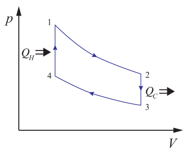
Figure 1: The Otto engine cycle, made of two adiabatic strokes and two isochoric heat transfers.

• Process $1\rightarrow 2$ is an adiabatic expansion, the power stroke, where the engine does work while dropping in temperature.

• Process $2\rightarrow 3$ is an isochoric heat exchange, where a quantity $Q_{C}$ of heat leaves the system, resulting in a further temperature drop.

• Process $3\rightarrow 4$ is an adiabatic compression, resulting in a temperature increase.

• Process $4\rightarrow 1$ is an isochoric heat exchange, where a quantity $Q_{H}$ of heat enters the system.

How the engine is realized depends upon the precise system, and the control parameters available. Overall, however, there’s a quantum thermodynamics description of the energy of the system (see e.g. refs.[29, 30, 3]) in terms of $\rho$ and ${\cal H}$, the state and Hamiltonian: $U{=}{\rm Tr}[\rho{\cal H}]$. Work on or by the system corresponds to changing ${\cal H}$. For example, for a harmonic oscillator it would amount to adjusting the basic frequency $\omega$ governing the spacing of the energy levels $E_{n}{=}(n+\frac{1}{2})\hbar\omega(t)$. Such a coupling is tunable in the laboratory (it might be set by the physical geometry of a resonator, or by the fields in an ion trap, or by the inductance or capacitance of a conducting microcircuit, etc). Heat flow to or from the system comes from the $\rho$ changing in response to the coupling to the environment. Formally, on average these are:

$$\langle W\rangle=\int_{t_{i}}^{t_{f}}{\rm Tr}[\rho^{(t)}{\dot{\cal H}}^{(t)}]dt\ ,\quad{\rm and}\quad\langle Q\rangle=\int_{t_{i}}^{t_{f}}{\rm Tr}[{\dot{\rho}}^{(t)}{\cal H}^{(t)}]dt\ ,$$ (1)

In this language the meaning of an adiabatic change of the parameter (performed in steps 1-2 and 4-1) is that the precise pattern of energy occupation is unchanged, which is achievable for slow enough (isolated) evolution. That the changing parameter maps directly to volume changes follows from the first law, using that we’re on an adiabat: $dS{=}0$. For the harmonic oscillator, changes in $\omega$ map to changes in volume, with $V\sim\omega^{-1}$. Expansion (compression) corresponds to a reduction (increase) in the basic oscillator frequency $\omega$ between the values $\omega_{h}$ and $\omega_{c}$, where $\omega_{h}>\omega_{c}$. This identification of a volume change with a change in a basic coupling in the quantum system is an important clue for how to interpret the effective thermodynamic volume in gravitational systems, as we’ll discuss later.

The precise details of the heat exchange are also system dependent. In all cases they amount to putting the system into thermal contact with a larger system that can act as a sink or source of heat. An extremely common way to model this is to write ${\dot{\rho}}^{(t)}$ in terms of a coupling of $\rho$ to operators of Lindblad type[2], representing the environment, but this is not the only approach (see refs. [3] for a review.).

For the quantum harmonic oscillator, if the cycles can be performed extremely slowly, so as to achieve perfect adiabaticity and frictionless thermalization, all energy changes can be written in terms of overall frequency changes or population changes. Then the total work done amounts to[31] $W=\hbar\Delta\omega\Delta N$, where $\Delta\omega=\omega_{h}-\omega_{c}$ and $\Delta N=\Delta N_{h}=\Delta N_{c}$ is the population change along the isochores. This is the difference in heat flow, $W=Q_{H}-Q_{C}$, and so the efficiency is simply:

$$\eta=1-\frac{\omega_{c}}{\omega_{h}}=1-\frac{V_{1}}{V_{2}}\ .$$ (2)

If $\omega_{c}/\omega_{h}$ is chosen as $T_{C}/T_{H}$ then $\eta=\eta_{\rm C}^{\phantom{C}}$, the Carnot efficiency, but otherwise it is smaller. Either way, this is the ideal situation. Much of the study of quantum heat engines is concerned with modelling the non–ideal situation, especially the coupling mechanisms by which thermalization (perhaps with friction effects) takes place, working at finite power, and so on.

3 Black Holes

A key lesson from the previous section is that we need a system with an equation of state that allows for adiabatic processes that are independent of isochoric processes. This might seem like an obvious statement, but it is the central question here, since the simplest black holes (static, pure geometry) such as Schwarzschild and Reissner–Nordström solutions, do not have this independence. The entropy, $S$, given by a quarter of the area of the horizon, is a simple power of the horizon radius (denoted $r_{+}$ in what follows). The thermodynamic volume $V$ is given by the geometric (naive) volume of the space occupied by the black hole, which is also a power of $r_{+}$. Therefore isochores and adiabats are the same[32, 21]. In other words, we cannot use these black holes to make Otto engines.

The above observation is equivalent to saying that those black holes has the constant volume specific heat $C_{V}=0$. Since in a sense, $C_{V}$ is a direct measure of the available degrees of freedom (at least the traditional ones that can be excited without making volume changes), we see that Reissner–Nordström, Schwarzschild, (and various other simple static black holes), do not have any usable degrees of freedom for our purposes.

The answer lies in studying black holes whose thermodynamic volume $V$ is independent of the entropy $S$. These are slightly more complicated, but readily available. The simplest one is probably the Kerr–AdS black hole, obtained by adding a rotation parameter. The appearance of the resulting conserved angular momentum, $J$ in the thermodynamic parameters ensures that $C_{V}\neq 0$. Another choice is the family of “STU” black holes in AdS. These are charged black holes that are coupled to four $U(1)$ gauge fields (and three scalars) in an asymmetric way. The familiar Reissner–Nordström black hole is a special case where the charges $Q_{i}$ ($i=1,\cdots 4$) are all equal (and the scalars decouple) and the Schwarzschild black hole is the special case where the charges $Q_{i}$ are all zero. The black hole solutions, the associated thermodynamic variables, and the resulting equations of state, are all reviewed in the next two sections.

The key point in both of these classes of solution, observed in ref. [23], is as follows. An examination of the specific heat as temperature varies, $C_{V}(T)$, shows that it has (for a particular choice of volume) a peak at some finite $T$, and then a decrease to zero as $T$ grows. This is characteristic of a finite window of available energy states in the system. For Kerr–AdS (or the three–equal–charge STU–AdS examples, which we will focus on here) the peak’s position and height (a measure of the size of our subsystem) is controlled by $J$ (or $Q$).

Before proceeding, we note that the previous section has also provided a lesson/suggestion about the meaning of the extended gravitational thermodynamic volume, $V$. It has been a puzzle as to what it means in the context of holographically dual field theory, with some suggestions made in the literature[14, 21, 38, 39, 40, 41]. Here, we see that untangling it from the entropy, combined with trying to make contact with quantum heat engines has opened up a new possibility: It is an effective coupling, somewhat analogous to how the 1D harmonic oscillator’s frequency $\omega$ acts as an inverse volume parameter for the thermodynamics, as we reviewed in the previous section. Much of what we do in the rest of this paper will be consistent with this as a natural interpretation, although it would be fruitful to try to prove the correspondence directly in the dual field theory.

3.1 Kerr–AdS Black Holes

For our first exhibit with $C_{V}\neq 0$, let us turn to the Kerr–AdS spacetime, which has metric[42, 43]:

$$ds^{2} = -\frac{\Delta}{\rho^{2}}\left(dt-\frac{a\sin^{2}\theta}{\Xi}d\phi\right)^{2}+\frac{\rho^{2}}{\Delta}dR^{2}+\frac{\rho^{2}}{\Delta_{\theta}}d\theta^{2}+\frac{\Delta_{\theta}\sin^{2}\theta}{\rho^{2}}\left(adt-\frac{R^{2}+a^{2}}{\Xi}\right)^{2}\ ,$$ (3)

$${\rm with}\quad\Delta\equiv\frac{(R^{2}+a^{2})(\ell^{2}+R^{2})}{\ell^{2}}-2mR\ ,\quad\Delta_{\theta}\equiv 1-\frac{a^{2}}{\ell^{2}}\cos^{2}\theta\ ,$$

$${\rm and}\quad\rho^{2}\equiv R^{2}+a^{2}\cos^{2}\theta\ ,\quad\Xi\equiv 1-\frac{a^{2}}{\ell^{2}}\ .$$

(Here we are working in four dimensions, for clarity.) The horizon at $R_{+}$ is the largest solution of $\Delta(R_{+})=0$. The quantities:

$$M=m/\Xi^{2}\ ,\quad{\rm and}\quad J=aM$$ (4)

are the physical mass and angular momentum, respectively. The entropy is a quarter of the area of the horizon, $S=\pi(R_{+}^{2}+a^{2})/\Xi$, but the thermodynamic volume turns out to be independent of $S$[44]. It is hard to write the equation of state $T(p,V)$ in closed form, but the mass, and a bit of algebra, yields the enthalpy in the form $H(S,p,J){=}M$, from which $T(S,p,J)$, and $V(S,p,J)$, are readily derived[45, 46]:

$$H(S,p,J) = \frac{1}{2}\sqrt{\frac{\left(S+\frac{8pS^{2}}{3}\right)^{2}+4\pi^{2}\left(1+\frac{8pS}{3}\right)J^{2}}{\pi S}}\ ,$$ (5)

$$T(S,p,J) = \frac{1}{8\pi H}\left[\left(1+\frac{8pS}{3}\right)\left(1+8pS\right)-4\pi^{2}\left(\frac{J}{S}\right)^{2}\right]\ ,$$ (6)

$$V(S,p,J) = \frac{2}{3\pi H}\left[S\left(S+\frac{8pS^{2}}{3}\right)+2\pi^{2}J^{2}\right]\ .$$ (7)

3.2 STU Black Holes

The STU–AdS metric is (again, working in four dimensions for presentational clarity)[47, 48, 49]:

$$ds^{2} = -(H_{1}H_{2}H_{3}H_{4})^{-1/2}f(r)dt^{2}+(H_{1}H_{2}H_{3}H_{4})^{1/2}\left(f(r)^{-1}dr^{2}+r^{2}(d\theta^{2}+\sin^{2}\theta d\phi^{2})\right)\ ,$$ (8)

$${\rm with}\quad f(r)\equiv 1-\frac{2m}{r}+\frac{r^{2}}{\ell^{2}}H_{1}H_{2}H_{3}H_{4}\ ,$$

and the functions $H_{i}=(1+q_{i}/r)$ are given in terms of four parameters $q_{i}$ ($i=1,\cdots,4$). The horizon is at $r=r_{+}$, where $r_{+}$ is given by $f(r_{+})=0$. This equation determines the parameter $m$ in terms of $q_{i}$ and $r_{+}$:

$$m=\frac{r_{+}}{2}\left(1+\frac{r_{+}^{2}}{\ell^{2}}\prod_{i}H_{i}(r_{+})\right)\ .$$ (9)

Then the extended thermodynamics yields[40] the following expressions for the enthalpy $H$, as well as $T,S,V$, and $p$:

$$H = M=m+\frac{1}{4}\sum_{i}q_{i}\ ,$$ (10)

$$T = \frac{f^{\prime}(r_{+})}{4\pi}\prod_{i}H_{i}^{-1/2}(r_{+})\ ,$$ (11)

$$S = \pi\prod_{i}\sqrt{r_{+}+q_{i}}\ ,$$ (12)

$$V = \frac{\pi}{3}r_{+}^{3}\prod_{i}H_{i}(r_{+})\sum_{j}H_{j}^{-1}(r_{+})\ ,$$ (13)

$$p = \frac{3}{8\pi G\ell^{2}}\ .$$ (14)

The parameters $q_{i}$ are related to a family of four physical charges that are given by

$$Q_{i}=\frac{1}{2}\sqrt{q_{i}(q_{i}+2m)}\ .$$ (15)

In the special case of all four charges being equal, the scalars decouple, and the solution becomes Reissner–Nordström–AdS, with $Q=\sum_{i}Q_{i}/4$.

This leads to a nice picture: choices that break the symmetry to give the more general STU holes are akin to a sort of “doping” process. Degrees of freedom (resulting in a finite energy window) are added to the system resulting in $C_{V}\neq 0$. This is somewhat analogous to the sort of doping one might do in a material, resulting in Schottky peaks in the experimental data.

For simplicity, we will restrict ourselves in this paper to the case of three equal charges, which we will sometimes denote as 3-$Q$ (Reissner–Nordström is 4-$Q$ in this notation).

3.3 Schottky–like peaks, and a Critical point

For both types of black hole, Kerr–AdS and the 3-$Q$ STU black hole, the overall phase structure is qualitatively similar to the van–der Waals structure discovered for 4-$Q$ in ref.[50]. Figure 2 displays a family of isotherms showing that there is a critical temperature $T_{c}$ at which an unstable (positive slope) region develops which is in fact excluded by a family of first order transitions (indicated by the green horizontal lines). We will avoid the first order region in all that we do in this paper, for simplicity, but the neighbourhood of the critical point will be of interest to us for two reasons. The first reason is that, as observed in ref. [23], the peak of the Schottky–like behaviour is also in the neighbourhood of the critical point (note that the round top of the peak is accessible above $T_{c}$). See figure 2 for an example of $C_{V}(T)$. The second reason will emerge in section 5.

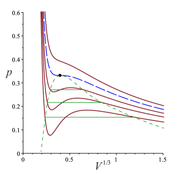
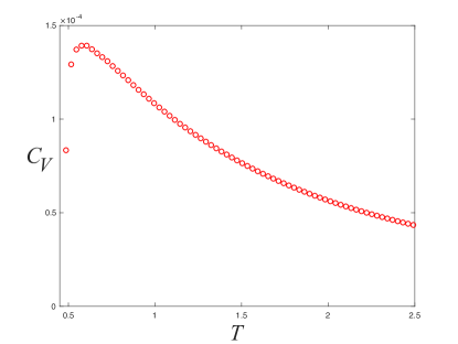
Figure 2: (a) A family of isotherms showing the appearance of the critical region as temperature is decreased toward $T_{c}$ (indicated by the (blue) long–dashed isotherm. There are first order transitions below that temperature. See the text. (b) The specific heat $C_{V}(T)$ at $V\simeq 4.166V_{c}$, showing a Schottky–like peak somewhat above $T_{c}\simeq 0.539$ (this is the 3-$Q$ STU case, with $Q=0.05$).

It is worth pausing here to understand the nature and implications of the peak. It is central to our overall proposal. We do not have a direct path by which we can start with the dual gauge theory, find an interpretation there of the black hole’s thermodynamic volume, and then solve for the reduced model that results when working in the fixed volume ensemble. Whether that is possible or not is left for future research. However $C_{V}(T)$ is a very specific clue to the results of such a process. The peak is a clear earmark of a finite window of available energies for the effective system. The high temperature regime, which we have a clear sight of well away from the critical region, contains an exponential fall off of the form $\exp(-\Delta/k_{B}T)$ (where $\Delta$ is a characteristic energy scale of the problem), possibly multiplied by powers of $T$. The low temperature limit, generically obscured by the critical regime here, would have the same form, sending $C_{V}(T)\to 0$ as $T\to 0$ as is consistent with Nernst’s theorem. Two extremely simple (and highly relevant) models that have specific heats of this form are the Schottky specific heat for (say) a two–level system and a truncated quantum harmonic oscillator. The specific heat of the quantum harmonic oscillator, with energies $E_{n}=(n+\frac{1}{2})\hbar\omega$ is

$$C_{V}^{\rm QHO}=k_{B}\left(\frac{\Delta}{k_{B}T}\right)^{2}\frac{{\rm e}^{\beta\Delta}}{(1-{\rm e}^{\beta\Delta})^{2}}\ ,\qquad{\rm where}\quad\beta=\frac{1}{k_{B}T}\ ,\quad\Delta=\hbar\omega\ .$$ (16)

This is the classic 1907 model that Einstein used for modelling experimental features of specific heats[52], and is displayed in figure 3.

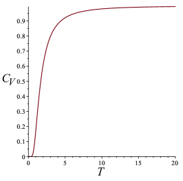
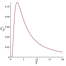
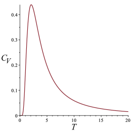
Figure 3: Three examples of the temperature dependence of the specific heat $C_{V}(T)$ (a) The quantum harmonic oscillator, with $\Delta=5$. (b) The quantum harmonic oscillator truncated to $n=5$. Here, $\Delta=1$. (c) A two–level Schottky model, with $\Delta=5$.

Notice that this specific heat has a representation as an infinite series:

$$C_{V}^{\rm QHO}=k_{B}\left(\frac{\Delta}{k_{B}T}\right)^{2}\sum_{n=1}^{\infty}n{\rm e}^{-n\beta\Delta}\ ,$$ (17)

and a truncation to any finite $n$ (effectively turning off the contributions above a certain excitation level) will result in a peak of the form under discussion. See figure 3. The classic Schottky specific heat for a two level system is closely related in form to the above, with (interestingly) a simple sign flip:

$$C_{V}^{\rm Schottky}=k_{B}\left(\frac{\Delta}{k_{B}T}\right)^{2}\frac{{\rm e}^{\beta\Delta}}{(1+{\rm e}^{\beta\Delta})^{2}}=k_{B}\left(\frac{\Delta}{k_{B}T}\right)^{2}\sum_{n=1}^{\infty}(-1)^{n-1}n{\rm e}^{-n\beta\Delta}\ ,$$ (18)

where here $\Delta$ is the energy gap between the levels. This is depicted in figure 3.

The point is that these analytic forms of the peaks match well to the “phenomenologically” discovered [23] peaks (see e.g. figure 2). While we do not have a direct derivation of it from first principles, we see that our physics has a spectrum with a finite energy window, which corresponds to some truncated spectrum (either continuous or discrete), with an associated scale $\Delta$. This is our working substance, and it is fully modelled by the equations of state supplied by the black holes. It compares well to the types of simple quantum systems (spins, harmonic oscillators, etc.,) used in theoretical and experimental studies of quantum heat engines.

4 Otto Engines from Black Holes

Now we are ready to construct an Otto cycle. The goal is to locate the $(p,V,T)$ coordinates of the four points of the cycle (1,2,3,4, as shown in figure 1), and then compute the efficiency of the engine.

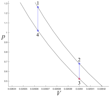
Figure 4: An Otto engine cycle for the 3-$Q$ STU-AdS black hole, where corner 3 is at $(p_{c},V_{c})$. Labelling matches that in figure 1.

This requires the determination of the heat flows $Q_{H}$ ($4\to 1$) and $Q_{C}$ ($2\to 3$). This can be done by explicitly integrating $C_{V}(T)dT$ along the isochores. Alternatively, there is a more direct result that can be used because the black hole organizes the thermodynamic variables quite nicely. Since the First Law is $dU=TdS-pdV$, movement along an isochore means that the heat can be simply written as the change in internal energy, and hence:

$$\eta=1-\frac{U_{2}-U_{3}}{U_{1}-U_{4}}\ ,\quad{\rm where}\quad U=H-pV\ ,$$ (19)

and $H$ is simply the black hole mass (see eqns. (4) and (10)). This equation is the natural analogue of the simple formula written in ref.[26] using masses for cycles where all heat exchanges are on isobars. The second law of thermodynamics ensures that $\eta\leq\eta_{\rm C}$, the Carnot efficiency (made by constructing a Carnot engine operating between heat baths at the highest ($T_{1}$) and lowest ($T_{3}$) temperatures) and is given by:

$$\eta_{\rm C}^{\phantom{C}}=1-\frac{T_{3}}{T_{1}}\ .$$ (20)

4.1 STU Black Hole Otto

In practice, since we do not have closed forms for the thermodynamic quantities, our exact formula cannot be used to avoid numerical methods. So, as described in ref. [23], once a region of interest in state space has been identified, an $n\times n$ grid of points (typically for $n=100$) was chosen (in the $(p,V)$ plane), over which all the state functions of interest ($T$, $S$, $U$, etc.,) were computed numerically. The results were then stored for later data mining when analyzing the heat engines. (We used both Maple and MatLab to do this.)

The strategy for proceeding was to pick the coordinates of a starting corner ($(p_{3},V_{3})$ say, see figure 1). The value of the state functions such as $S,T,H$, or $U$ can then be mined from the numerical data. Of course $V_{2}=V_{3}$ since corner 2 is on an isochore. The other two choices to make in order to define the cycle are the value of $p_{2}$, and the value of $V_{4}=V_{1}$. The pressures $p_{1}$ and $p_{4}$ follow from the fact that they lie on adiabats connecting to the corners 3 and 2, and so they must be determined, again using the numerical data since adiabats are not known in closed form. Now all corners have their coordinates determined, and so state variables (such as $T,H$ or $U$) can then be mined from the data.

Figure 4 is an example of an Otto cycle constructed in this way using the 3-$Q$ black hole (with $Q=0.05$). We chose to place the corner $(p_{3},V_{3})$ at the critical point, $(p_{c}\simeq 0.5240,V_{c}\simeq 0.026400)$. We chose $p_{2}\simeq 0.6812$ and $V_{1}\simeq 0.026363$. (The extra digits on volumes are a reflection of the fact that the adiabats are just slightly off being the vertical lines of the $C_{V}=0$ case for this small choice of $Q$.) The efficiency of this prototype Otto cycle turns out to be $\eta=0.2625$, while the Carnot efficiency is $\eta_{\rm C}^{\phantom{C}}\simeq 0.3387$, setting the upper bound, by the second law of thermodynamics.

4.2 Kerr Black Hole Otto

Fortunately, some analytic progress on our Otto engine can be made for the Kerr black hole. The expression for the volume $V$ in equation (7) can be used to solve for $p$ in terms of $(V,S,J)$ and so $p$ can be eliminated from $H$ to give[46]:

$$H(S,V,J)=\frac{1}{2}\sqrt{\left\{\left(\frac{3V}{4\pi}\right)^{2}-\left(\frac{S}{\pi}\right)^{3}\right\}^{-1}\left[\left\{\left(\frac{S}{\pi}\right)^{2}+2J^{2}\right\}^{2}-\left(\frac{S}{\pi}\right)^{2}\left\{\left(\frac{S}{\pi}\right)^{2}+4J^{2}\right\}\right]}$$ (21)

Then, $U=H-pV$ can be constructed and written in terms of its natural variables as[46]:

$$U(S,V,J)=\left(\frac{\pi}{S}\right)^{3}\left[\left(\frac{3V}{4\pi}\right)\left\{\frac{1}{2}\left(\frac{S}{\pi}\right)^{2}+J^{2}\right\}-J^{2}\left\{\left(\frac{3V}{4\pi}\right)^{2}-\left(\frac{S}{\pi}\right)^{3}\right\}^{\frac{1}{2}}\right]\ .$$ (22)

From this $T(S,V,J)=(\partial U/\partial S)_{V}$ can be written directly, and it is:

$$T=\frac{3J^{2}}{\pi}\left(\frac{\pi}{S}\right)^{4}\left[\left\{\left(\frac{3V}{4\pi}\right)^{2}-\frac{1}{2}\left(\frac{S}{\pi}\right)^{3}\right\}\left\{\left(\frac{3V}{4\pi}\right)^{2}-\left(\frac{S}{\pi}\right)^{3}\right\}^{-\frac{1}{2}}-\left(\frac{3V}{4\pi}\right)\left\{1+\frac{3}{18J^{2}}\left(\frac{S}{\pi}\right)^{2}\right\}\right]\ .$$ (23)

This is an extremely convenient pair of thermodynamic functions to write, and in terms of $S$ and $V$ especially, since the Otto cycle is indeed built from adiabats and isochores and so is represented in an $(S,V)$ diagram as a rectangle (see figure 5). We need only choose, say, $(S_{3},V_{3})$

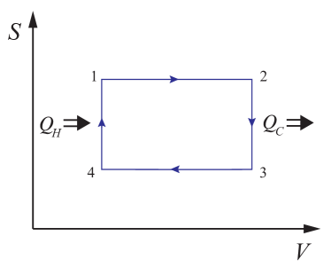
Figure 5: The Otto engine cycle in the $(S,V)$ plane. Labelling matches that in figure 1.

and $(S_{1},V_{1})$ and we can write the efficiency down fully by substituting the values into equation (22) to get the $U_{i}$, ($i=1,2,3,4$), and then computing equation (19). The Carnot efficiency bound (20) for that engine is also easily computed by using the chosen values at corners 1 and 3 to compute $T_{1}$ and $T_{3}$. In either case, the expressions for $\eta$ and $\eta_{\rm C}$ are readily written down and are too large to write usefully in single expressions.

Another natural plane to work in is the $p{-}S$ plane, since expressions (5), (7), and (6) are written naturally with that dependence. Again, analytic expressions can be written for the efficiencies using these formulae, albeit too long to write usefully here.

There is a tradeoff, however. With both choices of independent variables ($(S,V)$ or $(p,S)$), picking coordinates of the corners such that the equations of state are satisfied becomes a delicate matter. This is traceable to our central feature—the fact that $C_{V}$ is very small. So it requires some care to ensure that the corners can be connected by adiabats, and this again requires the equations of state to be solved numerically.

For stability, it turned out again that it was convenient to do the numerical work in the $p{-}V$ plane (by eliminating $S$ from equations (5), (7), and (6) to obtain $T(p,V)$ and $S(p,V)$) and using the scheme of the previous section. In this way, we found solutions very similar in structure to that seen in figure 4, extracting $\eta$ and $\eta_{\rm C}^{\phantom{C}}$. We will discuss more of this in the next section.

Having the form of $U(S,V)$ explicitly (22) means that we can use the exact formula (19) to deduce some important features of our engine. We can write $U=v[1/2s+J^{2}(1-\alpha)/s^{3})]$, where $s=S/\pi$ and $v=3V/4\pi$ and $\alpha=\sqrt{1-s^{3}/v^{2}}$, which vanishes when $J=0$. The heat $Q_{C}=U_{2}-U_{3}$ at the isochore $V_{2}$ is simply $Q_{C}=v_{2}[1/2s_{2}-1/2s_{3})+J^{2}K_{2}]$, where $K_{2}$ comes from evaluating the difference of the order $J^{2}$ terms. Similarly $Q_{H}=v_{1}[1/2s_{1}-1/2s_{4})+J^{2}K_{1}]$, where $K_{1}>K_{2}$. Since $s_{1}=s_{2}$ and $s_{1}=s_{4}$, we can divide by an overall constant $\beta=(s_{4}-s_{1})/2s_{1}s_{4}$ to write the ratio of heats as $Q_{C}/Q_{H}=V_{2}/V_{1}(1-J^{2}(K_{1}-K_{2})/\beta+\cdots)$, where we treat $J$ as small. At $J=0$, adiabats return to being vertical and $V_{1}\to V_{2}$, the engine has zero area and $\eta\to 0$. The difference $K_{1}{-}K_{2}$ vanishes at $J=0$ and must increase with the ratio $V_{1}/V_{2}$ in such a way that $\eta$ must remain positive (lest we violate the first law), and the rate at which it increases depends upon $J$, since $J$ controls the shape of the adiabats. A reasonable guess as to the dependence that satisfies these conditions at this order is $K_{1}{-}K_{2}=(\beta/J^{2})[1-(V_{1}/V_{2})^{\gamma}]$, where $\gamma>1$. This gives (in the small $J$ regime where we expect to make contact with a quantum heat engine):

$$\eta=1-\left(\frac{V_{1}}{V_{2}}\right)^{\gamma-1}\left(1+O(J^{2})\right)\ .$$ (24)

(We checked explicitly that this power law behaviour for $1{-}\eta$ is indeed borne out in fully (numerically) solved examples for small $J$.) This form of the efficiency is the classic form for the traditional Otto engine, but additionally, it agrees with the form for certain simple quantum Otto engines as well, for a variety of simple working substances[53]. (For the 1D harmonic oscillator example reviewed in section 2, $\gamma=2$.) Here, the constant $\gamma$ is the effective adiabatic exponent $C_{p}/C_{V}$. It is an effective adiabatic exponent because while we expect a finite $\gamma$ because now $C_{V}\neq 0$, since both $C_{p}$ and $C_{V}$ vary over the $p{-}V$ plane (as independent functions), and hence $\gamma$ varies. In our case $\gamma$ is very large (of order $10^{3}$ for the types of engines we built in the numerical examples discussed below), reflecting that we have chosen to have a very small number of degrees of freedom.

While equation (24) is a satisfying form for the outcome, this result also points to a limiting feature of our examples chosen thus far. We have worked with $J$ small, in order to be in a regime where we studying the thermodynamics of a “small” subsector of the usual large $N$ dynamics gravity gives access to. On the other hand, $J$ also controls the degree to which we can separate adiabats from isochores, so making it small gives us a large adiabatic exponent, which is not representative of most working substances. (A similar story is likely true for the STU Otto engines, controlled by $Q$.) Were the goal to simply reproduce efficiency formulae, we would stop at this point. The larger goal, however, as stated in the introduction, is to find a setting where we might be able to usefully interrogate a range of issues concerning quantum heat engines, independently of the size of $\gamma$, and the proposal is that we have.

5 Running Near Criticality

With $J$ (or $Q$) available as a free parameter, it is an interesting question as to how its value affects the Otto engine’s performance. Allied to this question is the issue of whether the neighbourhood of the critical point can have an effect on the efficiency. This matter arose in the quantum heat engine literature in the context of finding schemes by which the power of a heat engine might be enhanced, while retaining high efficiency. It was suggested[24] that if the working substance had the right kind of critical point, an enhancement could be achieved, principally because the specific heat gets an enhancement at such a critical point. In fact, this was tested in the holographic heat context in ref.[25] and shown to be qualitatively correct, although the heat engine there was not of the Otto type we are considering here. So it is interesting to revisit that scenario now that we have Otto engines. We do not expect an enhancement here, however. This is because the critical point for our working substance (modelled by the black hole) gives a divergence in $C_{p}$, not $C_{V}$, and it is the latter that is in play for Otto engines. So with no interesting features like a critical point for the constant volume degrees of freedom, we’d expect that there should be no $J$–dependence for the ratio, and we will see that this expectation is borne out.

Mimicing the setup of ref.[25], the idea is to keep the engine cycle always adjacent to the critical point, and then to study the dependence of the efficiency $\eta$ on $J$ (or $Q$). It is natural to compare to the Carnot efficiency of that same engine, and so we study the ratio $\eta/\eta_{\rm C}^{\phantom{C}}$. For simplicity, and because there was much greater numerical control of the equations of state, we will focus on the case of the Kerr Otto engine, but our results for the STU Otto engines were similar. The position of the critical point is given, for small $J$ by[54]:

$$p_{c}=\frac{1}{12\pi(90)^{1/2}}\frac{1}{J}\ ,\quad S_{c}=\pi(90)^{1/4}J\ ,\quad V_{c}=\frac{4\pi}{3}(90)^{3/4}J^{3/2}\ ,\quad T_{c}=\frac{(90)^{3/4}}{225\pi}\frac{1}{J^{1/2}}\ .$$ (25)

To make the comparison at different values of the $J$, we chose a region of the plane of a size that scaled with the location with the critical point (e.g., the lower bound on $p$ and $S$ was $p_{c}/4$ and $S_{c}/4$, respectively, and upper bound was $2p_{c}$ and $6S_{c}$). We numerically solved the equations of state there. Picking the corners $(p_{3},V_{3})=(p_{c},V_{c})$ and $(p_{2},V_{2})=(3p_{c}/2,V_{c})$ (see labelling in figure 4 or figure 1) we numerically solved the adiabat from there to find the largest $p_{1}$ that would fit into the chosen region. We then found the corresponding $V_{1}=V_{4}$, determining the termination point when solving the adiabat that runs from corner 3. Knowledge of the coordinates of corners 1 and 3 were enough to determine the temperatures there and hence $\eta_{\rm C}^{\phantom{C}}$.

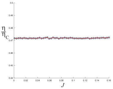
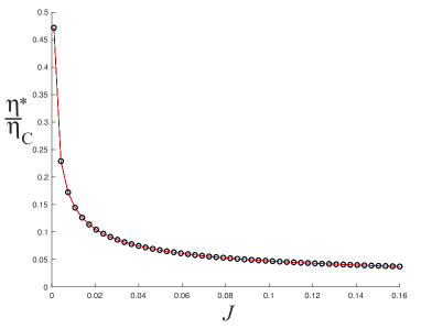
Figure 6: (a) The ratio of the efficiency of the (Kerr black hole) Otto engine to its Carnot efficiency. (b) The ratio of the rescaled (see text) efficiency of the (Kerr black hole) Otto engine to its Carnot efficiency.

Our results are in figure 6 and 6, and the heat flows and work performed were computed by both direct integration along each branch of the cycle, and by computing differences in $U$, as a check of our methods. We see in figure 6 that $\eta/\eta_{C}^{\phantom{C}}$ retains a constant (within numerical error) value of $\sim 0.472$ as $J$ varies over the range $(0.001,0.16)$. This confirms the expectation expressed above.

An engine of a given design can be made more efficient by simply making it larger i.e., allowing it to occupy a larger area in the $p{-}V$ plane. Our choice of how we placed the engine near the critical point, described above, amounts to a work that scales as $W\sim J^{1/2}$ (this follows from the scaling of $p_{c}$ and $V_{c}$ and we verified this by computing the work at each $J$). We can have a different measure of the relative performance if instead we rescale the efficiencies such that they are all normalized to the same fixed work $W^{*}$, giving $\eta^{*}=\eta\,\,(W^{*}/W)$, where $W^{*}$ was chosen as the work at $J=0.001$. In this way the scheme becomes closer to that in ref.[25], where the work was held constant when comparing different charges. The ratio $\eta^{*}/\eta_{C}^{\phantom{C}}$ would be expected to fall as $1/J^{1/2}$, and this is confirmed by the result shown in figure 6.

6 Brayton and Diesel Cycles

It is straightforward to construct other classic engine cycles. The two most obvious to consider are the Brayton cycle and the Diesel cycle, sketched in figures 7 and 7 respectively.

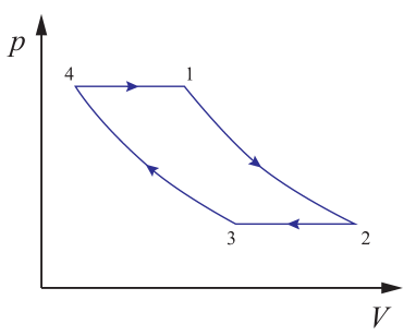
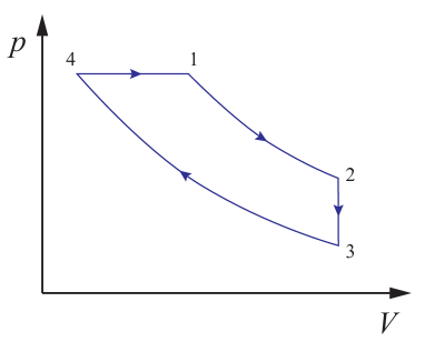
Figure 7: (a) The Brayton cycle, made from two isobars and two adiabats. (b) The Diesel cycle made from two adiabats, an isobar, and an isochore.

It is interesting to consider black hole versions of these cycles in the context of this paper because there have been quantum heat engine constructions that use these cycles (see the discussion in refs. [30, 53]). An appealing feature of these engines is that we again can use the fact that the gravitational thermodynamics so readily supplies the enthalpy $H$ as the mass $M$ of the black hole, from which the volume is readily derived and so $U{=}H{-}pV$ is straightforward to compute, as mentioned in earlier sections. Since the first law is $dH{=}TdS{+}Vdp$ or $dU{=}TdS{-}pdV$ and we have heat exchanges on either isobars or isochores, all heat exchanges can be written as either $H$ differences or $U$ differences. So the efficiencies are readily written as:

$$\eta_{\rm B}^{\phantom{B}}=1-\frac{H_{2}-H_{3}}{H_{1}-H_{4}}\ ,\quad{\rm and}\quad\eta_{\rm D}^{\phantom{D}}=1-\frac{U_{2}-U_{3}}{H_{1}-H_{4}}\ .$$ (26)

The first is the exact formula of ref.[26] and they both are natural counterparts to equation (19).

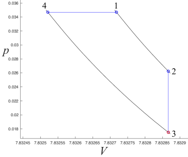
Figure 8: A Diesel engine cycle for the $J=0.16$ Kerr-AdS black hole, where corner 3 is at $(p_{c},V_{c})$. Labelling matches that in figure 7.

Using these it was straightforward to construct some examples using as working substance the Kerr and STU black holes presented here, using techniques similar to those we employed in section 4. See figure 8 for an example of a Diesel engine made from a Kerr black hole, computed at $J=0.16$, with $\eta\simeq 0.2216$ and $\eta_{\rm C}^{\phantom{C}}\simeq 0.2903$.

While these were interesting to construct (at least as proof of concept) there is a key reason why they are perhaps less compelling than our Otto black hole engines: For the isobaric components the heat exchanges involve the large number of degrees of freedom (scaling like a positive power of $N$) that can be excited in fixed pressure processes. In other words, the dual quantum system is the unrestricted large $N$ gauge theory, not the small window afforded by the fixed volume processes (see subsection 3.3). Therefore the thermodynamics involves a rather classical system on those branches. This makes less compelling any argument that these are quantum heat engines (in the sense alluded to in subsection 1.2). At best, perhaps Diesel is a hybrid sort of system, with a small system on the isochoric part and large on the isobaric part. It is possible that such a large$+$small hybrid may well be of interest, maybe even experimentally, in the quantum heat engine context, so it is worth observing that they can arise naturally as black hole models.

7 Discussion

Two key features formed the foundation of this paper’s proposal. The first is that extended gravitational thermodynamics provides solvable models of equations of state for systems that have known (for $\Lambda<0$) underlying microscopic quantum descriptions, because of holographic duality. The second is that constant volume processes have a highly reduced window of energy excitations[23], suggesting that the dynamics in play is that of a system that is (tunably) “small” compared to the full (“large $N$”) number of degrees of freedom usually described by these gravity duals. Putting this together, as done here, holographic heat engines that employ this reduced system would seem to define models of quantum heat engines. We showed that the black hole Otto cycle, presented here for the first time, has exceedingly interesting properties in this regard. This connection may be of use because it enriches the family of quantum heat engines that have been defined so far, and —perhaps more importantly— provides an entirely new laboratory of techniques for exploring the thermodynamics of small quantum systems.

It would be interesting to explore this connection further, and there are many fruitful avenues along which to depart. Besides constructing more examples (there is a host of black hole solutions of various types, in various dimensions, that have $C_{V}\neq 0$) it would be interesting to directly employ the underlying quantum description (i.e., holography) to explore features of the engines. An effective field theory model of the reduced system that operates at fixed thermodynamic volume would be useful in this regard, and it can presumably be derived directly from the holographically dual field theory. (It may begin with a system of, possibly truncated, quantum harmonic oscillators in some number of dimensions, given the observations in section 3.3. Perhaps the thermodynamic volume their inverse effective frequency, generalizing the 1–dimensional case reviewed in section 2.) The thermalization process that happens at constant volume may be illuminated by studying the evolution of the entanglement entropy. This is again something that is accessible in the holographic description, using the techniques of refs.[55, 56], suitably adapted to constant volume processes. As mentioned in section 1.2, getting at the underlying quantum features of the system in this way may be useful for addressing the issue of how quantum heat engines differ from their classical counterparts in certain regimes, such as considering operation at finite power.

The quantum heat engine models that are accessible using our construction are in general likely to be somewhat more complex (or simple, depending upon point of view) than those that have been extensively studied in the literature so far. (It would be an unexpected, though pleasant, surprise to be able to model a pure two–level spin system with a black hole, for example.) As discussed in section 4.2, this is partly due to the fact that we have selected a small number of degrees of freedom out a very large parent system, resulting in very large $\gamma=C_{p}/C_{V}$. It would be of interest to try to see if there are gravitational models with more parameters that can help avoid this limitation, giving access to the small $\gamma$s (of order 1) of familiar materials while retaining the small system limit. This does not mean that the construction may not be a useful laboratory for testing ideas and even modelling phenomena seen in experiments.

Indeed, since quantum heat engines are of considerable active experimental interest, with new realizations appearing regularly in a range of contexts (spin systems, trapped ions, resonant cavities, etc.), the working substances being used will become increasingly more intricate, and may well yield exotic behaviours. A holographic heat engine description via black holes may well prove useful for understanding their features, perhaps in ways analogous to how large $N$ models gave useful insights into strongly coupled aspects of nuclear physics, and condensed matter physics.

References

- [1] H. E. D. Scovil and E. O. Schulz-DuBois, “Three-level masers as heat engines,”Phys. Rev. Lett. 2 (Mar, 1959) 262–263. https://link.aps.org/doi/10.1103/PhysRevLett.2.262.
- [2] H. Breuer and F. Petruccione, The Theory of Open Quantum Systems. Oxford University Press, 2002. https://books.google.com/books?id=qVGZAQAACAAJ.
- [3] S. Vinjanampathy and J. Anders, “Quantum thermodynamics,” Contemporary Physics 57 (2016) no. 4, 545–579. https://doi.org/10.1080/00107514.2016.1201896.
- [4] N. Y. Halpern, Quantum steampunk: Quantum information, thermodynamics, their intersection, and applications thereof across physics. PhD thesis, Caltech, 2018. arXiv:1807.09786 [quant-ph].
- [5] J. D. Bekenstein, “Black holes and entropy,” Phys.Rev. D7 (1973) 2333–2346.
- [6] J. D. Bekenstein, “Generalized second law of thermodynamics in black hole physics,” Phys.Rev. D9 (1974) 3292–3300.
- [7] S. Hawking, “Particle Creation by Black Holes,” Commun.Math.Phys. 43 (1975) 199–220.
- [8] S. Hawking, “Black Holes and Thermodynamics,” Phys.Rev. D13 (1976) 191–197.
- [9] S. W. Hawking and D. N. Page, “Thermodynamics of Black Holes in anti-De Sitter Space,” Commun. Math. Phys. 87 (1983) 577.
- [10] G. ’t Hooft, “Dimensional reduction in quantum gravity,” in Salamfest 1993:0284-296, pp. 0284–296. 1993. arXiv:gr-qc/9310026 [gr-qc].
- [11] J. M. Maldacena, “The large n limit of superconformal field theories and supergravity,” Adv. Theor. Math. Phys. 2 (1998) 231–252, hep-th/9711200.
- [12] E. Witten, “Anti-de sitter space and holography,” Adv. Theor. Math. Phys. 2 (1998) 253–291, hep-th/9802150.
- [13] S. S. Gubser, I. R. Klebanov, and A. M. Polyakov, “Gauge theory correlators from non-critical string theory,” Phys. Lett. B428 (1998) 105–114, hep-th/9802109.
- [14] D. Kastor, S. Ray, and J. Traschen, “Enthalpy and the Mechanics of AdS Black Holes,” Class.Quant.Grav. 26 (2009) 195011, arXiv:0904.2765 [hep-th].
- [15] S. Wang, S.-Q. Wu, F. Xie, and L. Dan, “The First laws of thermodynamics of the (2+1)-dimensional BTZ black holes and Kerr-de Sitter spacetimes,” Chin.Phys.Lett. 23 (2006) 1096–1098, arXiv:hep-th/0601147 [hep-th].
- [16] Y. Sekiwa, “Thermodynamics of de Sitter black holes: Thermal cosmological constant,” Phys.Rev. D73 (2006) 084009, arXiv:hep-th/0602269 [hep-th].
- [17] E. A. Larranaga Rubio, “Stringy Generalization of the First Law of Thermodynamics for Rotating BTZ Black Hole with a Cosmological Constant as State Parameter,” arXiv:0711.0012 [gr-qc].
- [18] M. Henneaux and C. Teitelboim, “The Cosmological Constant as a Canonical Variable,” Phys.Lett. B143 (1984) 415–420.
- [19] M. Henneaux and C. Teitelboim, “The Cosmological Constant and General Covariance,” Phys.Lett. B222 (1989) 195–199.
- [20] C. Teitelboim, “The Cosmological Constant as a Thermodynamic Black Hole Parameter,” Phys.Lett. B158 (1985) 293–297.
- [21] C. V. Johnson, “Holographic Heat Engines,” Class. Quant. Grav. 31 (2014) 205002, arXiv:1404.5982 [hep-th].
- [22] C. V. Johnson and F. Rosso, “Holographic Heat Engines, Entanglement Entropy, and Renormalization Group Flow,” Class. Quant. Grav. 36 (2019) no. 1, 015019, arXiv:1806.05170 [hep-th].
- [23] C. V. Johnson, “Specific Heats and Schottky Peaks for Black Holes in Extended Thermodynamics,” arXiv:1905.00539 [hep-th].
- [24] M. Campisi and R. Fazio, “The power of a critical heat engine,” Nat. Commun. 7 (2016) 11895, arXiv:1603.05024 [cond-mat.stat-mech].
- [25] C. V. Johnson, “Exact model of the power-to-efficiency trade-off while approaching the Carnot limit,” Phys. Rev. D98 (2018) no. 2, 026008, arXiv:1703.06119 [hep-th].
- [26] C. V. Johnson, “An Exact Efficiency Formula for Holographic Heat Engines,” Entropy 18 (2016) 120, arXiv:1602.02838 [hep-th].
- [27] A. Chakraborty and C. V. Johnson, “Benchmarking Black Hole Heat Engines, II,” Int. J. Mod. Phys. D27 (2018) no. 16, 1950006, arXiv:1709.00088 [hep-th].
- [28] R. A. Hennigar, F. McCarthy, A. Ballon, and R. B. Mann, “Holographic heat engines: general considerations and rotating black holes,” Class. Quant. Grav. 34 (2017) no. 17, 175005, arXiv:1704.02314 [hep-th].
- [29] T. D. Kieu, “Quantum heat engines, the second law and maxwell’s daemon,”The European Physical Journal D - Atomic, Molecular, Optical and Plasma Physics 39 (Jul, 2006) 115–128, arXiv:quant-ph/0311157 [quant-ph].
- [30] H. T. Quan, Y.-x. Liu, C. P. Sun, and F. Nori, “Quantum thermodynamic cycles and quantum heat engines,”Phys. Rev. E 76 (Sep, 2007) 031105, arXiv:quant-ph/0611275 [quant-ph].
- [31] Y. Rezek and R. Kosloff, “Irreversible performance of a quantum harmonic heat engine,”New Journal of Physics 8 (may, 2006) 83–83, arXiv:quant-ph/0601006 [quant-ph]. https://doi.org/10.1088%2F1367-2630%2F8%2F5%2F083.
- [32] B. P. Dolan, “The cosmological constant and the black hole equation of state,” Class.Quant.Grav. 28 (2011) 125020, arXiv:1008.5023 [gr-qc].
- [33] M. Banados, C. Teitelboim, and J. Zanelli, “The Black hole in three-dimensional space-time,” Phys. Rev. Lett. 69 (1992) 1849–1851, arXiv:hep-th/9204099 [hep-th].
- [34] M. Banados, M. Henneaux, C. Teitelboim, and J. Zanelli, “Geometry of the (2+1) black hole,” Phys. Rev. D48 (1993) 1506–1525, arXiv:gr-qc/9302012 [gr-qc]. [Erratum: Phys. Rev.D88,069902(2013)].
- [35] C. Martinez, C. Teitelboim, and J. Zanelli, “Charged rotating black hole in three space-time dimensions,” Phys. Rev. D61 (2000) 104013, arXiv:hep-th/9912259 [hep-th].
- [36] S. Gunasekaran, R. B. Mann, and D. Kubiznak, “Extended phase space thermodynamics for charged and rotating black holes and Born-Infeld vacuum polarization,” JHEP 1211 (2012) 110, arXiv:1208.6251 [hep-th].
- [37] A. M. Frassino, R. B. Mann, and J. R. Mureika, “Lower-Dimensional Black Hole Chemistry,” Phys. Rev. D92 (2015) no. 12, 124069, arXiv:1509.05481 [gr-qc].
- [38] B. P. Dolan, “Bose condensation and branes,” JHEP 10 (2014) 179, arXiv:1406.7267 [hep-th].
- [39] D. Kastor, S. Ray, and J. Traschen, “Chemical Potential in the First Law for Holographic Entanglement Entropy,” JHEP 11 (2014) 120, arXiv:1409.3521 [hep-th].
- [40] E. Caceres, P. H. Nguyen, and J. F. Pedraza, “Holographic entanglement entropy and the extended phase structure of STU black holes,” JHEP 09 (2015) 184, arXiv:1507.06069 [hep-th].
- [41] J. Couch, W. Fischler, and P. H. Nguyen, “Noether charge, black hole volume, and complexity,” JHEP 03 (2017) 119, arXiv:1610.02038 [hep-th].
- [42] B. Carter, “Hamilton-Jacobi and Schrodinger separable solutions of Einstein’s equations,” Commun. Math. Phys. 10 (1968) no. 4, 280–310.
- [43] J. Plebanski and M. Demianski, “Rotating, charged, and uniformly accelerating mass in general relativity,” Annals Phys. 98 (1976) 98–127.
- [44] M. Cvetic, G. Gibbons, D. Kubiznak, and C. Pope, “Black Hole Enthalpy and an Entropy Inequality for the Thermodynamic Volume,” Phys.Rev. D84 (2011) 024037, arXiv:1012.2888 [hep-th].
- [45] M. M. Caldarelli, G. Cognola, and D. Klemm, “Thermodynamics of Kerr-Newman-AdS black holes and conformal field theories,” Class.Quant.Grav. 17 (2000) 399–420, arXiv:hep-th/9908022 [hep-th].
- [46] B. P. Dolan, “Pressure and volume in the first law of black hole thermodynamics,” Class.Quant.Grav. 28 (2011) 235017, arXiv:1106.6260 [gr-qc].
- [47] W. A. Sabra, “Anti-de Sitter BPS black holes in N=2 gauged supergravity,” Phys. Lett. B458 (1999) 36–42, arXiv:hep-th/9903143 [hep-th].
- [48] M. J. Duff and J. T. Liu, “Anti-de Sitter black holes in gauged N = 8 supergravity,” Nucl. Phys. B554 (1999) 237–253, arXiv:hep-th/9901149 [hep-th].
- [49] M. Cvetic, M. J. Duff, P. Hoxha, J. T. Liu, H. Lu, J. X. Lu, R. Martinez-Acosta, C. N. Pope, H. Sati, and T. A. Tran, “Embedding AdS black holes in ten-dimensions and eleven-dimensions,” Nucl. Phys. B558 (1999) 96–126, arXiv:hep-th/9903214 [hep-th].
- [50] A. Chamblin, R. Emparan, C. V. Johnson, and R. C. Myers, “Charged AdS black holes and catastrophic holography,” Phys. Rev. D60 (1999) 064018, hep-th/9902170.
- [51] D. Kubiznak and R. B. Mann, “P-V criticality of charged AdS black holes,” JHEP 1207 (2012) 033, arXiv:1205.0559 [hep-th].
- [52] A. Einstein, “Die plancksche theorie der strahlung und die theorie der spezifischen wärme,” Annalen der Physik 327 (1907) no. 1, 180–190.
- [53] H. T. Quan, “Quantum thermodynamic cycles and quantum heat engines. ii.,”Phys. Rev. E 79 (Apr, 2009) 041129, arXiv:0811.2756 [quant-ph].
- [54] N. Altamirano, D. Kubiznak, R. B. Mann, and Z. Sherkatghanad, “Thermodynamics of rotating black holes and black rings: phase transitions and thermodynamic volume,” Galaxies 2 (2014) 89–159, arXiv:1401.2586 [hep-th].
- [55] S. Ryu and T. Takayanagi, “Holographic derivation of entanglement entropy from AdS/CFT,” Phys.Rev.Lett. 96 (2006) 181602, arXiv:hep-th/0603001 [hep-th].
- [56] S. Ryu and T. Takayanagi, “Aspects of holographic entanglement entropy,” JHEP 08 (2006) 045, arXiv:hep-th/0605073.
- [57] C. V. Johnson, “Black Holes and Quantum Heat Engines,” in KITP Conference: Open Quantum Systems in Quantum Simulators (Apr 29 - May 3, 2019). http://online.kitp.ucsb.edu/online/qsim-c19/johnson/.