Sensitivity computation of statistically stationary quantities in turbulent flows

Abstract

It is well-known that linearized perturbation methods for sensitivity analysis, such as tangent or adjoint equation-based, finite difference and automatic differentiation are not suitable for turbulent flows. The reason is that turbulent flows exhibit chaotic dynamics, leading to the norm of an infinitesimal perturbation to the state growing exponentially in time. As a result, these conventional methods cannot be used to compute the derivatives of long-time averaged quantities to control or design inputs. The ensemble-based approaches [1, 2] and shadowing-based approaches ([3, 4, 5]) to circumvent the problems of the conventional methods in chaotic systems, also suffer from computational impracticality and lack of consistency guarantees, respectively. We introduce the space-split sensitivity, or the S3 algorithm, which is a Monte Carlo approach to the chaotic sensitivity computation problem. In this work, we derive the S3 algorithm under simplifying assumptions on the dynamics and present a numerical validation on a low-dimensional example of chaos.

1 Nomenclature

$d$	phase space dimension
$u$	a phase point or a state vector in $\mathbb{R}^{d}$
$u_{n}$	state vector at time $n$ starting from an initial state $u_{0}$
$F(u,s)$	a parameterized discrete-time system representing chaotic dynamics;
	The parameter is $s$
$J$	a scalar objective function of interest
$\mu^{s}$	an ergodic, invariant probability distribution of SRB type
$\langle J,(\partial\mu^{s}/\partial s)\rangle$	required sensitivity
$F^{i}_{uj}$	the product of Jacobians at $u_{j+i-1},u_{j+i-2},\cdots,u_{j}$, in this order: $F_{u(j+i-1)}F_{u(j+i-2)}\cdots F_{uj}$;
	the identity operator when $i=0$
$d_{u},d_{s}$	dimension of the unstable and stable subspaces respectively
$E^{\rm u}(u),E^{\rm s}(u)$	unstable and stable tangent subspaces at a phase point $u$, respectively
$V^{k}_{n}$	$k$-th tangent covariant Lyapunov vector (CLV) corresponding to the
	Lyapunov exponent (LE) $\lambda^{k}$ at the phase point $u_{n}$
$W^{k}_{n}$	$k$-th adjoint CLV corresponding to the LE $\lambda^{k}$ at the phase point $u_{n}$
$N^{\prime}$	number of timesteps for time correlation decay
$N$	number of samples or length of primal trajectory

2 Introduction

With recent advances in large-scale computing, high-fidelity simulations, such as large eddy simulations or direct numerical simulations of turbulent flow, are becoming increasingly common in aerodynamic modelling. Eddy-resolving simulations are predicted to become critical in the near future for design of next-generation aero-engines and turbomachinery wherein there is a greater demand for reduction in noise and pollutant emissions and higher efficiency [6, 7, 8]. Such examples call for an in-depth resolution of transition phenomena, shear instabilities, heat transfers, separations and so on, that require DNS/LES. Sensitivity analysis in these high-fidelity simulations is as yet undeveloped. In comparison, gradient information on RANS simulations and non-chaotic Navier-Stokes simulations have greatly benefited uncertainty quantification [9, 10], mesh adaptation [11], flow control [12], noise reduction [13, 14, 15] and aerostructural design optimization applications [16, 17, 18, 19, 20]. The gradients are computed in these simulations in the traditional way – from the solution of tangent or adjoint equations.

In the context of sensitivity analysis, chaotic simulations pose unique challenges. Since the instantaneous quantities in chaotic systems are stochastic in nature, meaningful objectives for design optimization and other applications are long-time averages of observables such as lift, drag, pressure loss, heat transfer etc. To compute the derivatives of long-time averages to changes in system inputs, one would conventionally use tangent or adjoint methods. But, the solution of linearized perturbation equations (including those obtained, with no numerical error, through automatic differentiation for instance) all have exponentially increasing norms in time – unbounded growth of infinitesimal perturbations to the state is a property of chaotic dynamics. An early approach, known as ensemble sensitivity computation, due to Lea et al. [1], proposed to take the sample average of short time sensitivities computed using these linearized perturbation equations. However, the ensemble sensitivity approach is computationally intractable, as some studies have shown [21, 2]. The more recent shadowing-based approaches [4, 22, 23, 3, 5] tackle this problem by numerically computing the shadowing perturbation solution, a carefully constructed tangent or an adjoint solution that remains bounded over a long time window. These approaches have been successfully applied to 3D flows over a cylinder [23]. However, there are some examples [24] where the approach has been shown to not converge to the correct sensitivity. In this work, we propose an alternative algorithm – space-split sensitivity (S3) – to obtain the sensitivity of infinite-time averages or equivalently, statistical averages in chaotic systems.

In the next section, we describe some mathematical prerequisites for the S3 algorithm. In section 5, we derive the algorithm for the simplistic case of one unstable Lyapunov exponent. Section 6 presents the algorithm in full and numerical results validating S3 on a low-dimensional example of chaos is discussed in section 7.

3 Problem Setup

The primal problem is the numerical simulation of a parameterized turbulent fluid flow. We assume it is of the form,

$$u_{n+1}=F(u_{n},s),\quad n=0,1,\cdots,\;\;u_{n}\in\mathbb{R}^{d}.$$ (1)

With $u_{0}$ as an initial flow field, the function $F$ takes in $u_{n}$, the flow field at timestep $n$, to produce the flow field at the next timestep $n+1$. The function $F$ represents the spatially and temporally discretized flow solver, with $s\in\mathbb{R}$ being a scalar parameter of the flow (e.g., inlet Mach number, a shape parameter of an airfoil etc). We use $J$ to denote a scalar objective function of interest, e.g., lift/drag in a flow over an airfoil, pressure loss in a turbine wake etc. The observed value at timestep $n$ of $J$ is denoted as $J_{n}$. The primal simulation resolves chaotic timescales. Consequently, a time-average of $J$, given by $\langle J\rangle_{N}:=(1/N)\sum_{n=0}^{N-1}J_{n}$ that is observable and is of engineering interest (in e.g., design and optimization) corresponds to a large $N$. We are interested in the sensitivity of the infinite-time average of $J$ to a small change in $s$. That is, we want to compute the quantity $d(\lim_{N\to\infty}\langle J\rangle_{N})/ds$.

4 Mathematical background

The goal of this section is to present some mathematical prerequisites for the derivation of the S3 algorithm. The present treatment is not meant to be rigorous (the reader is referred to [25] for a detailed exposition) but rather a brief, intuitive explanation of some concepts from dynamical systems and ergodic theory, to the extent applicable to the developments in the further sections.

4.1 Phase space perspective

The flow field at time $n$, $u_{n}$, is a point in a $d$-dimensional phase space, denoted by ${\cal M}$. Each dimension corresponds to a degree of freedom in the flow simulation. For instance, in a 3D incompressible flow where we solve for the 3 velocity components and the pressure at every grid point, the dimension of the phase space $d$ is equal to $4$ times the number of grid points. Each unsteady flow simulation sequentially visits a finite number of points in ${\cal M}$ – a finite length trajectory in phase space. The set of all trajectories in phase space converges to a closed and bounded set in $\mathbb{R}^{d}$. This set, called an attractor, contains the asymptotic trajectories of all points starting from initial conditions in the neighbourhood of the set.

We are interested in statistically stationary flows i.e., fluid flows in which the state vector has achieved a time-invariant probability distribution on the attractor. That is, each trajectory (flow simulation) samples a finite number of phase points (state vectors) distributed according to an invariant probability distribution. An ensemble average refers to taking an expected value according to this distribution; thus, it is the operation of taking the sample average at phase points on the attractor in the limit as the number of samples goes to infinity.

4.2 Linearized perturbation equations and uniform hyperbolicity

The tangent space at a phase point $u$, denoted by $T_{u}{\cal M}$, is a $d$-dimensional vector space, that consists of all possible infinitesimal perturbations to the state. Each tangent vector gives a direction of perturbation; given a scalar function on the phase space, the tangent vector provides a valid direction to compute the directional derivative of the scalar function along. In this paper, we deal with a class of idealized dynamical systems, called uniformly hyperbolic systems. In uniformly hyperbolic systems, the tangent space at every point can be decomposed into stable and unstable, lower dimensional subspaces, denoted by $E^{\rm s}$ and $E^{\rm u}$ respectively – $T_{u}{\cal M}=E^{\rm u}(u)\oplus E^{\rm s}(u)$. It is important to note that this decomposition is a direct sum decomposition, not an orthogonal decomposition. Roughly speaking, uniform hyperbolicity is the existence of a stable-unstable decomposition of the tangent space on the attractor that is covariant (i.e., stable (unstable) vectors are mapped to stable (unstable) vectors under the tangent dynamics along a primal trajectory) with the dynamics.

We will now introduce the tangent dynamics, which essentially track the evolution of infinitesimal perturbations linearized about a primal trajectory. The familiar tangent equation for the evolution of an infinitesimal perturbation to the parameter, $\zeta_{n}:=\frac{\partial u_{n}}{\partial s}$ (at a fixed primal initial condition $u_{0}$), is given by,

$$\zeta_{n+1} =F_{un}\zeta_{n}+F_{sn},$$ (2)

$$\zeta_{0} =0\in\mathbb{R}^{d},$$ (3)

where $F_{un}$ is the Jacobian matrix consisting of the partial derivatives of the form $\partial F^{(i)}/\partial u^{(j)}$, evaluated at the phase point $u_{n}$; the superscript $(i)$ indicates the i-th Cartesian coordinate. Following a similar notation, $F_{sn}$ indicates the partial derivative $\partial F/\partial s$, evaluated at the phase point $u_{n}$, at a reference value of the parameter $s$. Note that $F_{sn}$ is a tangent vector belonging to the tangent space at $u_{n+1}$, $T_{u_{n+1}}{\cal M}$; this is clear from Eq.2 where it can be subtracted from $\zeta_{n+1}$, a tangent vector in $T_{u_{n+1}}{\cal M}$. We denote by $X_{n}$ the tangent vector of the source term in the previous timestep, i.e., $X_{n}:=F_{s(n-1)}\in T_{u_{n}}{\cal M}$.

The homogeneous tangent equation gives the evolution of an infinitesimal perturbation to the initial state. That is, let $\zeta_{0}\in T_{u_{0}}{\cal M}$ and $u_{0}^{\prime}=u_{0}+\epsilon\zeta_{0}$. Then, keeping $s$ fixed at a reference value,

$$\zeta_{n}:=\partial u_{n}/\partial\epsilon=\lim_{\epsilon\to 0}\frac{u_{n}^{\prime}-u_{n}}{\epsilon},$$

where $u_{n}^{\prime}$ is the state at time $n$ starting with $u_{0}^{\prime}$ as the initial condition. The tangent vector $\zeta_{n}$ satisfies the following tangent equation,

$$\zeta_{n+1}=F_{un}\zeta_{n},$$ (4)

which is called the homogeneous tangent equation since it is the conventional tangent equation with the source term zero. We are now ready to define uniform hyperbolicity more precisely using the behavior of linearized perturbation solutions. To wit, in uniformly hyperbolic systems, there exist constants $C>0$ and $\lambda\in(0,1)$ such that for every initial condition $u_{0}$, if $\zeta_{0}\in E^{\rm s}(u_{0})$, then, the solution of the homogeneous tangent equation (Eq.4), $\zeta_{n}\in E^{\rm s}(u_{n})$ and $\lVert\zeta_{n}\rVert\leq C\lambda^{n}\lVert\zeta_{0}\rVert$, for all $n>0$. Similarly, if $\zeta_{0}\in E^{\rm u}(u_{0})$, then, the solution of the homogeneous tangent equation (Eq.4) backward in time (using the inverse Jacobian $F_{un}^{-1}$), $\zeta_{-n}\in E^{\rm u}(u_{-n})$ and $\lVert\zeta_{-n}\rVert\leq C\lambda^{n}\lVert\zeta_{0}\rVert$, for all $n>0$.

Suppose $J$ is a scalar-valued state function. The conventional adjoint equation gives the backward evolution of the derivative of $J$ at time $N$, denoted as $J_{N}$, to an infinitesimal perturbation to the state $u_{n}$. The familiar adjoint equation for $\xi_{n}:=\partial J_{N}/\partial u_{n}$, is given by,

$$\xi_{n} =F_{un}^{T}\xi_{n+1}+{\rm grad}_{n}\left(J_{n}\right),\;\;n=N,N-1,\cdots,$$ (5)

$$\xi_{N+1} =0\in\mathbb{R}^{d},$$ (6)

where ${\rm grad}_{n}\left(J_{n}\right)$ is the gradient of the function $J$ evaluated at $u_{n}$. Setting the source term of the above equation to zero, we get the following homogeneous adjoint equation,

$$\xi_{n} =F_{un}^{T}\xi_{n+1}.$$ (7)

In a uniformly hyperbolic system, we can also write down a different decomposition of the tangent space at a phase point classifying tangent vectors that decay or grow exponentially in norm, under the homogeneous adjoint dynamics (Eq.7). This decomposition is related to the decomposition into $E^{\rm u}$ and $E^{\rm s}$. If $\xi_{n}$ is a stable adjoint vector, that is, $\xi_{n}\in T^{*}_{u_{n}}{\cal M}$ is such that $\lVert\xi_{0}\rVert\leq C\lambda^{n}\lVert\xi_{n}\rVert$, then, $\xi_{n}\in E^{{\rm u}^{\perp}}(u_{n})$. Similarly, one can show that unstable adjoint vectors are also covariant and belong to the orthocomplement of the stable tangent subspaces, $E^{{\rm s}^{\perp}}$. Thus, the decomposition based on stable and unstable adjoint vectors at a phase point is given by $T^{*}_{u}{\cal M}=E^{{\rm u}^{\perp}}(u)\oplus E^{{\rm s}^{\perp}}(u)$.

4.3 Covariant Lyapunov vectors

Covariant Lyapunov vectors (CLVs), denoted by $V^{1},\cdots,V^{d}$ form a special non-orthogonal basis for the tangent space at every point. Here $V^{1},\cdots,V^{d}$ denote the normalized basis vectors. The CLV basis is covariant in the sense that if $\zeta_{0}:=V^{k}_{0}\in T_{u_{0}}{\cal M}$ is an initial condition of the homogeneous tangent equation (Eq.4), then, the solution at time $n$, $\zeta_{n}\in{\rm span}\{V^{k}_{n}\}$, for each $k=1,\cdots,d$. Moreover, the asymptotic logarithmic growth rates of the CLVs are independent of the primal initial condition and are the so-called Lyapunov exponents. Equivalently, Lyapunov exponents can also be expressed as the ensemble average of the logarithmic growth rate of the CLVs. That is, the $k$-th Lyapunov exponent (LE), denoted by $\lambda^{k}$ is the ensemble average over initial conditions $u_{0}$ of, $\log(\lVert F_{u0}V^{k}_{0}\rVert/\lVert V^{k}_{0}\rVert)=\log(\lVert F_{u0}V^{k}_{0}\rVert)$. We assume that no two LEs are equal and index them in the descending order as, $\lambda^{1}>\lambda^{2}>\cdots>\lambda^{k}$. The adjoint CLVs have an analogous definition with the same LEs and the homogeneous adjoint equation replacing the role of the homogeneous tangent equation. We denote the normalized adjoint CLVs using $W^{1},\cdots,W^{d}$.

Furthermore, the tangent CLVs at $u$ corresponding to unstable homogeneous tangent solutions, i.e., $\lambda^{k}>1$, form a basis for $E^{\rm u}(u)$. If $d_{u}<d$ is the dimension of the unstable subspace (which is the same at every phase point) and $d_{s}=d-d_{u}$ is the dimension of the stable subspace, then, $E^{\rm u}(u)={\rm span}\{V^{1}(u),V^{2}(u),\cdots,V^{d_{u}}(u)\}$ and similarly, $E^{\rm s}(u)={\rm span}\{V^{d_{u}+1}(u),\cdots,V^{d}(u)\}$. The orthocomplements, $E^{{\rm u}^{\perp}}$ and $E^{{\rm s}^{\perp}}$, are spanned by the adjoint stable CLVs ($W^{k},k=d_{u}+1,\cdots,d$) and adjoint unstable CLVs ($W^{k},k=1,\cdots,d_{u}$) respectively.

4.4 Tangent-adjoint orthogonality property

Since the CLVs are tangent vectors, the orthogonality property of stable and unstable adjoint and tangent vectors, alluded to in section 4.2, applies to them. More explicitly, $W^{k}\in E^{{\rm s}^{\perp}}$ for $k=1,\cdots,d_{u}$ and $V^{j}\in E^{\rm s}$ for $j=d_{u}+1,\cdots,d$ and so, $W^{k}\cdot V^{j}=0$, at every phase point. In words, a stable tangent CLV is orthogonal to an unstable adjoint CLV at every point. Similarly, an unstable tangent CLV is orthogonal to a stable adjoint CLV. This orthogonality will be referred to as the tangent-adjoint orthogonality or TAO property.

4.5 Measure preservation

In statistically stationary systems, the assumption of uniform hyperbolicity guarantees the existence of a unique invariant probability distribution called the SRB distribution (see [26] for an introduction to SRB measures), that has certain convenient properties. Most importantly, it is a physically observable distribution, in the sense that, long time averages of functions along trajectories converge to their expected value according to the SRB distribution. That is, $\lim_{N\to\infty}\langle J\rangle_{N}:=\int J\;d\mu^{s}$, where $\mu^{s}$ is the SRB distribution, for almost every initial condition $u_{0}$. The superscript $s$ indicates the SRB distribution depends on the parameter $s$. The sensitivity we would like to compute can therefore be equivalently written as $d/ds(\lim_{N\to\infty}\langle J\rangle_{N})=d/ds(\int J\;d\mu^{s})=\int J\;d\mu^{s}/ds$.

Denoting the integral pairing $\int Jd\mu^{s}$ using $\langle J,\mu^{s}\rangle$, $\langle J_{0},\mu^{s}\rangle=\langle J_{n},\mu^{s}\rangle$, for any $n$, where, with a slight abuse of notation, $J_{i}$ denotes the function composition $J\circ F\circ(i\;{\rm times})\;\circ F$. That is, considering an ensemble of initial conditions, independent and identically distributed according to $\mu^{s}$, the average of a function $J$ over the primal trajectories starting from the ensemble, is independent of time. This statement essentially captures the statistical stationarity of the fluid flow with respect to the SRB distribution. In another interpretation, we can arbitrarily move the time origin to any time while computing ensemble averages with respect to an invariant distribution such as the SRB distribution. This property is called measure preservation property or MPP for short.

5 Derivation of the S3 algorithm

In this section, we derive the S3 algorithm for a uniformly hyperbolic chaotic system, placing emphasis on the physical/computational motivation for each step; the rigorous mathematical details of some steps of the derivation are left to the appendix. From Ruelle’s linear response theory (see [27, 28] for the derivation) the sensitivity of interest can be expressed through the following formula, where $X(u_{n})=X_{n}:=F_{s(n-1)}$,

$$\langle J,\dfrac{\partial\mu^{s}}{\partial s}\rangle =\sum_{n^{\prime}=0}^{\infty}\langle{\rm grad}_{0}\left(J_{n^{\prime}}\right)\cdot X,\mu^{s}\rangle.$$

We decompose the formula by writing the tangent vector $X=X^{\rm s}+X^{\rm u}$, as a sum of its stable and unstable components, i.e., $X^{\rm s}\in E^{\rm s}$ and $X^{\rm u}\in E^{\rm u}$ at every phase point. Then,

$$\langle J,\dfrac{\partial\mu^{s}}{\partial s}\rangle =\sum_{n^{\prime}=0}^{\infty}\langle{\rm grad}_{0}\left(J_{n^{\prime}}\right)\cdot X^{\rm s},\mu^{s}\rangle+\sum_{n^{\prime}=0}^{\infty}\langle{\rm grad}_{0}\left(J_{n^{\prime}}\right)\cdot X^{\rm u},\mu^{s}\rangle.$$ (8)

We refer to the two components of Eq.8 as the stable and unstable contributions, and denote them using the subscripts “stable” and “unstable” respectively. The stable contribution can be computed using the conventional tangent solution approach, as in a non-chaotic system. To see this, note that in the stable contribution, the summation and the ensemble-averaging operations can be commuted, since at almost every initial condition, the instantaneous sensitivity is bounded at all times. That is, the stable contribution can be written as

$$\langle J,\frac{\partial\mu^{s}}{\partial s}\rangle_{\rm stable} =\sum_{n^{\prime}=0}^{\infty}\langle{\rm grad}_{0}\left(J_{n^{\prime}}\right)\cdot X^{\rm s},\mu^{s}\rangle=\langle\sum_{n^{\prime}=0}^{\infty}{\rm grad}_{-n^{\prime}}\left(J_{0}\right)\cdot X^{\rm s}_{-n^{\prime}},\mu^{s}\rangle,$$ (9)

where the second equality is obtained by applying the MPP. Further, using the fact that the homogeneous tangent solution is stable for all time in this case,

$$\langle J,\frac{\partial\mu^{s}}{\partial s}\rangle_{\rm stable} =\sum_{n^{\prime}=0}^{\infty}\langle(F_{u(-n^{\prime})}^{n^{\prime}})^{T}{\rm grad}_{0}\left(J_{0}\right)\cdot X^{\rm s}_{-n^{\prime}},\mu^{s}\rangle=\sum_{n^{\prime}=0}^{\infty}\langle{\rm grad}_{0}\left(J_{0}\right)\cdot F_{u(-n^{\prime})}^{n^{\prime}}X^{\rm s}_{-n^{\prime}},\mu^{s}\rangle$$ (10)

$$=\langle{\rm grad}_{0}\left(J_{0}\right)\cdot\sum_{n^{\prime}=0}^{\infty}F_{u(-n^{\prime})}^{n^{\prime}}X^{\rm s}_{-n^{\prime}},\mu^{s}\rangle=\langle{\rm grad}_{0}\left(J_{0}\right)\cdot\psi_{0}^{\rm s},\mu^{s}\rangle,$$ (11)

where $\psi_{0}^{\rm s}$ is the series summation of the homogeneous tangent solutions. In practice, it can be computed from solving a stable inhomogeneous tangent equation, the conventional tangent equation with a stable source term at every timestep. Explicitly, suppose $\zeta_{n}^{\rm s}$ is the solution to the following equation,

$$\zeta_{n+1}^{\rm s} =F_{un}\zeta_{n}^{\rm s}+X^{\rm s}_{n+1},\;\;n=0,1,\cdots,$$

$$\zeta_{0}^{\rm s} =X_{0}^{\rm s}\in\mathbb{R}^{d}.$$ (12)

Then, the stable contribution can be written approximately as the following ergodic average,

$$\langle J,\frac{\partial\mu^{s}}{\partial s}\rangle_{\rm stable} \approx\frac{1}{N}\sum_{n=0}^{N-1}{\rm grad}_{n}\left(J_{n}\right)\cdot\psi_{n}^{\rm s}\approx\frac{1}{N}\sum_{n=0}^{N-1}{\rm grad}_{n}\left(J_{n}\right)\cdot\zeta_{n}^{\rm s}.$$ (13)

The approximation $\psi_{n}^{\rm s}\approx\zeta_{n}^{\rm s}$ in Eq.13 gets better with $n$. From an explicit expression for the stable tangent solution $\zeta_{n}^{\rm s}=\sum_{n^{\prime}=0}^{n}F_{u(n-n^{\prime})}^{n^{\prime}}X^{\rm s}_{(n-n^{\prime})}$, we can see that it does not include the terms of the sequence $\left\{F_{u(n-n^{\prime})}^{n^{\prime}}X^{\rm s}_{(n-n^{\prime})}\right\},n^{\prime}=0,1,\cdots$ for $n^{\prime}>n$. But, since the sequence is exponentially decreasing in norm, the truncation error is insignificant at large $n$. Thus, the computation of the stable contribution resembles sensitivity computation in a non-chaotic system.

In deriving the computation of the unstable contribution, we now make the simplifying assumption that the unstable subspace is one-dimensional, i.e., $d_{u}=1$. Then the unstable contribution can be written as follows,

$$\langle J,\dfrac{\partial\mu^{s}}{\partial s}\rangle_{\rm unstable}=\sum_{n^{\prime}=0}^{\infty}\bigg{(}\langle x_{0}{\rm grad}_{0}\left(J_{n^{\prime}}\right)\cdot V_{0}^{1},\mu^{s}\rangle\bigg{)},$$ (14)

where the scalar field $x$ is the component of $X^{\rm u}$ along $V_{0}^{1}$. That is, $X^{\rm u}_{n}=x_{n}V_{n}^{1}$, along a trajectory. We seek an indirect computation of each summand that does not involve taking the derivative of $J_{n^{\prime}}$. We derive such a computation by establishing an iterative formula that is stable in the sense that its rate of convergence is uniformly bounded over $n^{\prime}$. The reader is referred to the Appendix section 8.2 for all the steps of the derivation. Here we will describe the mathematical intuition for why such a formula exists and how to compute it.

Roughly speaking, we argue that the computational constraints we have imposed direct us to an efficient approach. In particular, we seek an algorithm that scales linearly with $N$, the number of samples or the length of a trajectory used for a Monte Carlo approximation. Now note that each $n^{\prime}$ summand in the unstable contribution is a linear functional (an operation on a function that returns a scalar) on a suitable Hilbert space containing $J_{n^{\prime}}$. As a result of Riesz representation theorem, each $n^{\prime}$ summand has a representation as an inner product (on a Hilbert space of functions) of the objective function with another state function. That is, $\langle{\rm grad}_{0}\left(J_{n^{\prime}}\right)\cdot X_{0}^{\rm u},\mu^{s}\rangle=\langle J_{n^{\prime}}G^{\rm u}_{0},\mu^{s}\rangle$, where $G^{\rm u}$ is a scalar function and the right hand side of the equality is by definition the inner product. We will henceforth refer to $G^{\rm u}$ as the Riesz representation of unstable ensemble derivative (or RUED, for short). Note that the RUED does not capture the pointwise unstable derivative but rather its ensemble average, which is bounded for each $n^{\prime}$. The alternative representation afforded by the RUED is preferable for computation because it is able to show a Monte Carlo convergence as an ergodic average, as stipulated. This claim can be reasoned as follows. Suppose we have computed the RUED, $G^{\rm u}$, that satisfies $\langle J_{n^{\prime}}G^{\rm u}_{0},\mu^{s}\rangle=\langle{\rm grad}_{0}\left(J_{n^{\prime}}\right)\cdot X_{0}^{\rm u},\mu^{s}\rangle$. Then, the unstable contribution, upon applying the MPP, can be written as,

$$\langle J,\frac{d\mu^{s}}{ds}\rangle_{\rm unstable}=\sum_{n^{\prime}=0}^{\infty}\langle J_{0}G^{\rm u}_{-n^{\prime}},\mu^{s}\rangle.$$ (15)

Note that the $n^{\prime}$ summand is the time correlation at $n^{\prime}$ between the two state functions, $J$ and $G^{\rm u}$. State functions in uniformly hyperbolic systems, in general, enjoy an exponential decay of time correlations, i.e., Eq.15 converges exponentially with $n^{\prime}$ to the product of the ensemble averages of $J$ and $G^{\rm u}$. Therefore, in practice, when we compute the above expression (Eq.15) as an ergodic average, we can make an additional approximation,

$$\langle J,\frac{d\mu^{s}}{ds}\rangle_{\rm unstable}\approx\frac{1}{N}\sum_{n^{\prime}=0}^{\infty}\sum_{n=0}^{N-1}J_{n}G^{\rm u}_{n-n^{\prime}}\approx\frac{1}{N}\sum_{n=0}^{N-1}J_{n}\sum_{n^{\prime}=0}^{N^{\prime}-1}G^{\rm u}_{n-n^{\prime}},$$ (16)

where $N^{\prime}$ represents a timescale for the decay of correlations. Since $N^{\prime}$ is expected to be small in comparison to $N$, this results in a computation that scales roughly linearly with $N$, as we stipulated. Moreover, we expect the central limit theorem to be valid for the above $N$-sample estimator. This is in turn due to the fact that the variance in the random variable $J_{n^{\prime}}G^{\rm u}_{0}$ (the randomness comes from the initial condition) is uniformly bounded over $n^{\prime}$. In contrast, the variance of the integrand in the original form (Eq.17), ${\rm grad}_{0}\left(J_{n^{\prime}}\right)\cdot X_{0}^{\rm u}$, exhibits unbounded growth with $n^{\prime}$. Thus, an $N$-term ergodic average of Eq.17 shows a (much) slower convergence than the $1/\sqrt{N}$ convergence predicted by the central limit theorem (see [21] for an analysis of ensemble estimates of the gradient term).

The question remains as to how to compute the RUED, and is partially answered by integration by parts. Motivated to avoid the computation of a term such as ${\rm grad}_{0}\left(J_{n^{\prime}}\right)$, which is exponentially increasing in norm with $n^{\prime}$, we rewrite the unstable contribution as follows,

$$\langle J,\dfrac{\partial\mu^{s}}{\partial s}\rangle_{\rm unstable}=\sum_{n^{\prime}=0}^{\infty}\bigg{(}\langle{\rm grad}_{0}\left(x_{0}J_{n^{\prime}}\right)\cdot V_{0}^{1},\mu^{s}\rangle-\langle J_{n^{\prime}}{\rm grad}_{0}\left(x_{0}\right)\cdot V_{0}^{1},\mu^{s}\rangle\bigg{)}.$$ (17)

The above statement amounts to integration by parts which, as we expect, has a regularization effect. We can see that the second term above, which is in the form of a time correlation between the state functions $J$ and ${\rm grad}_{\cdot}\left(x\right)\cdot V_{\cdot}^{1}$, leads to a Monte Carlo method. We are now left with expressing the first term also as a time correlation in order to determine $G^{\rm u}$ completely. In the Appendix section 8.2, we determine a scalar field $\alpha^{\rm u}$ that satisfies $\langle{\rm grad}_{0}\left(x_{0}J_{n^{\prime}}\right)\cdot V_{0}^{1},\mu^{s}\rangle=\langle J_{n^{\prime}}\alpha^{\rm u},\mu^{s}\rangle$. By using the MPP and algebraic manipulations, we arrive at the following formula for $\alpha^{\rm u}$ (see Appendix section 8.2 for the full derivation),

$$\alpha^{\rm u}_{n} =x_{n}\sum_{n^{\prime}=-\infty}^{n-1}\frac{\phi_{n^{\prime}}}{\Pi_{i=n^{\prime}+1}^{n-1}\lVert F_{ui}V_{i}^{1}\rVert},$$ (18)

where $\phi_{n}:=-{\rm grad}_{n}\left(1/\lVert F_{un}V_{n}^{1}\rVert\right)$. One can see that $\alpha^{\rm u}_{n}\approx\beta^{\rm u}_{n}$, the solution of the following equation,

$$\beta^{\rm u}_{n+1} =\frac{\beta^{\rm u}_{n}x_{n+1}}{\lVert F_{un}V_{n}^{1}\rVert x_{n}}+x_{n+1}\phi_{n},\;\;n=0,1,2,\cdots$$ (19)

$$\beta^{\rm u}_{0} =\phi_{-1}x_{0}.$$ (20)

The above equation will be referred to as the RUED equation, since it computes the RUED term partially. Together with the contribution from the second term in Eq.17, we have the following computable formula for the RUED term,

$$G^{\rm u}_{n}=\alpha^{\rm u}_{n}-{\rm grad}_{n}\left(x_{n}\right)\cdot V_{n}^{1}.$$ (21)

The unstable contribution can then be expressed as the following ergodic average approximation of the time correlation between $J$ and $G^{\rm u}$,

$$\langle J,\frac{\partial\mu^{s}}{\partial s}\rangle_{\rm unstable}\approx\frac{1}{N}\sum_{n=0}^{N-1}J_{n}\sum_{n^{\prime}=n-N^{\prime}+1}^{n}G^{\rm u}_{n^{\prime}}.$$ (22)

Finally, combining the stable and unstable contributions, we obtain the overall sensitivity,

$$\langle J,\dfrac{\partial\mu^{s}}{\partial s}\rangle_{\rm unstable}+\langle J,\dfrac{\partial\mu^{s}}{\partial s}\rangle_{\rm stable} \approx\frac{1}{N}\sum_{n=0}^{N-1}\Bigg{(}J_{n}\sum_{n^{\prime}=n-N^{\prime}+1}^{n}G^{\rm u}_{n^{\prime}}+{\rm grad}_{n}\left(J_{n}\right)\cdot\zeta_{n}^{\rm s}\Bigg{)}.$$ (23)

6 The S3 algorithm

In this section, we describe the implementation of the computable formula in Eq.23 that was derived in the previous section 5. We detail the following stepwise procedure that results in the sensitivity of interest $\langle J,({\partial\mu^{s}}/{\partial s})\rangle$.

1. Primal and unstable CLV computation

   1. Choose a random initial condition $u_{0}$ and solve the primal problem in Eq.1 for a large ${\cal N}$, producing the trajectory $u_{0},u_{1},\cdots,u_{\cal N}$.

   2. Solve the homogeneous tangent equation 4 along the computed primal trajectory, by starting with a random initial condition $\zeta_{0}$, and normalizing the solution at each timestep. The resulting unit vectors $\zeta_{n}$ approximate the unstable CLVs $V^{1}_{n}$ accurately after some time $N_{\rm tan}$.

   3. Solve the homogeneous adjoint equation 7 backward in time, again dividing the adjoint solution by its norm at each timestep, starting with a random initial condition $\xi_{\cal N}$. The resulting unit solution vectors $\xi_{n}$ accurately approximate the unstable adjoint CLVs $W^{1}_{n}$ after performing this procedure for time $N_{\rm adj}$, i.e., $W^{1}_{n}$ are accurate for all $n\leq{\cal N}-N_{\rm adj}$.

   4. Shift the time origin to $N_{\rm tan}$. We have obtained the unstable tangent and adjoint CLVs $V_{n}^{1},W_{n}^{1}$ respectively, along the trajectory $u_{n},\;n=0,1,\cdots,{\cal N}-N_{\rm tan}-N_{\rm adj}$.

2. Stable-unstable pertubation splitting and the RUED term pre-computations

   1. Compute $c^{1}_{n}:=W^{1}_{n}\cdot V^{1}_{n}$, for all $n=0,1,\cdots,{\cal N}-N_{\rm tan}-N_{\rm adj}$.

   2. Compute $X_{n+1}=F_{sn}$ at each $n$ analytically if possible, or through finite difference. Also obtain $x_{n}=X_{n}\cdot W_{n}^{1}/c_{n}^{1}$. Then, obtain the stable-unstable decomposition of $X_{n}$: $X_{n}^{\rm u}=x_{n}V_{n}^{1}$ and $X_{n}^{\rm s}=X_{n}-X_{n}^{\rm u}$.

   3. Obtain part of the RUED term $-{\rm grad}_{n}\left(x_{n}\right)\cdot V_{n}^{1}$ by using a finite difference approximation of ${\rm grad}_{n}\left(x_{n}\right)$.

   4. Compute $\phi_{n}:=-{\rm grad}_{n}\left(1/\lVert F_{un}V_{n}^{1}\rVert\right)$ also as a finite difference approximation. We now have the source term for the RUED equation, $x_{n+1}\phi_{n}$, at all $n$.

3. Initializations for the Monte Carlo loop

   1. Choose the times $N_{\rm rued}$ and $N_{\rm tan,s}$ after which the approximation errors $\lvert\alpha_{n}^{\rm u}-\beta_{n}^{\rm u}\rvert$ and $\lVert\psi_{n}^{\rm s}-\zeta_{n}^{\rm s}\rVert$ corresponding to the RUED (Eq.19) and the stable tangent (Eq.12) equations respectively, are both within specified tolerances. Let the guess $N_{\rm rued}$ be the maximum of the two times. It can be refined as the two equations are solved in the loop to follow.

   2. Choose the time $N^{\prime}$ for the decay of correlations $\langle JG_{-n}^{\rm u},\mu^{s}\rangle$. Again, the time $N^{\prime}$ can be fine-tuned in the following $n$-loop, where the RUED terms $G_{n}^{\rm u}$ will be obtained. After sufficient iterations, plot on a semilog scale, the time correlation between $J$ and $G^{\rm u}$. If tol is a specified precision and $-\gamma$ and $\log{C}$ are the slope and intercept of the plot respectively, then $N^{\prime}=(1/\gamma)\log(C/\verb+tol+)$.

   3. The number of samples, $N$, that is to be used for the Monte Carlo estimate of the sensitivity reduces to $N={\cal N}-N_{\rm tan}-N_{\rm adj}-N_{\rm rued}-N^{\prime}$.

   4. Initialize the loop variable $n$ to $-N_{\rm rued}-N^{\prime}$. Set zero initial conditions for the stable tangent equation and the RUED equation: $\zeta^{\rm s}_{n}=0\in\mathbb{R}^{d}$ and $\beta^{\rm u}_{n}=0\in\mathbb{R}$.

   5. Initialize an $N^{\prime}$-long array $q$ to 0. This data structure will be used to compute time correlations for the unstable contribution.

   6. Initialize to 0 the stable and unstable sensitivity outputs: $\langle J,(\partial\mu^{s}/\partial s)\rangle_{\rm stable}=\langle J,(\partial\mu^{s}/\partial s)\rangle_{\rm unstable}=0$. They are to be updated in the following $n$-loop.

4. Monte Carlo approximation of the stable and unstable contributions

   1. Solve the RUED equation (Eq.19) for the spin-up time $N_{\rm rued}$, to obtain $\beta_{-N^{\prime}}^{\rm u}$.

   2. Solve the stable tangent equation (Eq.12) for the time $N_{\rm rued}+N^{\prime}$, to obtain $\zeta_{0}^{\rm s}$.

   3. Continue solving the RUED equation for $n=-N^{\prime},\cdots,-1$ and set $\alpha_{n}^{\rm u}=\beta_{n}^{\rm u}$. Compute $G^{\rm u}_{n}$ from Eq.21 and step 2.3, for each $n$, and use them to populate $q$. Perform the next steps, 4.4–4.6, for each $n=0,1,\cdots,N-1$.

   4. Advance the RUED equation by one timestep, obtaining $\beta_{n}^{\rm u}$. Then set $\alpha_{n}^{\rm u}=\beta_{n}^{\rm u}$. Compute $G_{n}^{\rm u}$ from Eq.21 and using step 2.3, and use it to replace the ($n$ modulo $N^{\prime}$)-th element of $q$.

   5. Advance the stable tangent equation (Eq.12) by one timestep to obtain $\zeta_{n}^{\rm s}$. Add ${\rm grad}_{n}\left(J_{n}\right)\cdot\zeta_{n}^{\rm s}/N$ to the stable contribution, $\langle J,(\partial\mu^{s}/\partial s)\rangle_{\rm stable}$.

   6. Add the elements of the array $q$ to obtain $q_{{\rm sum},n}=\sum_{n^{\prime}={n-N^{\prime}+1}}^{n}G^{\rm u}_{n^{\prime}}$. Update the unstable contribution, $\langle J,(\partial\mu^{s}/\partial s)\rangle_{\rm unstable}$ by adding $q_{{\rm sum},n}J_{n}/N$.

5. At the end of the $n$-loop, the overall sensitivity is given by $\langle J,(\partial\mu^{s}/\partial s)\rangle_{\rm stable}+\langle J,(\partial\mu^{s}/\partial s)\rangle_{\rm unstable}$.

7 Example computation

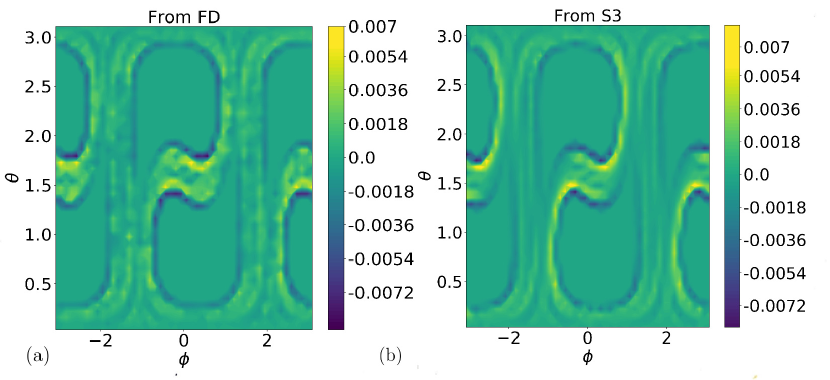
Figure 1: The sensitivity of the ensemble average of nodal basis functions to $s$ in the Kuznetsov-Plykin system. The results obtained from finite difference approximation and from S3 are shown on the left (a) and right (b) respectively.

In this section, we consider an example of a three-dimensional uniformly hyperbolic chaotic system. The reader is referred to Kuznetsov [29], wherein the dynamics is derived as that of a system of non-autonomous coupled oscillators and uniform hyperbolicity is numerically verified. Here we are interested in numerical results on this system, which we will refer to as the Kuznetsov-Plykin system, of the S3 algorithm derived in section 5. We consider the Kuznetsov-Plykin map on $u:=[x^{(1)},x^{(2)},x^{(3)}]^{T}\in\mathbb{R}^{3}$ written in Cartesian coordinates, given by,

$$u_{n+1}=F(u_{n},s)={\mathbf{f}}_{1,1}\circ\mathbf{f}_{-1,-1}(u_{n},s),$$ (24)

where the function ${\mathbf{f}_{\cdot,\cdot}}$ is specified in [29]. For completion, we repeat here the definition of ${\mathbf{f}}_{\cdot,\cdot}$, where the superscript $(k)$ indicates the Cartesian coordinate $k$,

$${\mathbf{f}}_{\sigma_{1},\sigma_{2}}^{(1)}(u,s)=\> \sigma_{2}\>x^{(3)}$$

$${\mathbf{f}}_{\sigma_{1},\sigma_{2}}^{(2)}(u,s)=\> \frac{\sqrt{x^{(1)^{2}}+x^{(2)^{2}}}}{\sqrt{x^{(1)^{2}}\>+\>x^{(2)^{2}}\exp{\left(2s(x^{(1)^{2}}\>+\>x^{(2)^{2}})\right)}}}\Big{[}\sigma_{1}\>x^{(1)}\>\>\sin{\left(\frac{\pi}{2}(\sqrt{2}x^{(3)}+1)\right)}$$

$$+\;x^{(2)}\exp{\left(s(x^{(1)^{2}}+x^{(2)^{2}})\right)}\>\cos{\left(\frac{\pi}{2}(\sqrt{2}x^{(3)}+1)\right)}\Big{]}$$

$${\mathbf{f}}_{\sigma_{1},\sigma_{2}}^{(3)}(u,s)= \frac{\sqrt{x^{(1)^{2}}+x^{(2)^{2}}}}{\sqrt{x^{(1)^{2}}\>+\>x^{(2)^{2}}\exp{\left(2s(x^{(1)^{2}}\>+\>x^{(2)^{2}})\right)}}}\Big{[}-\sigma_{2}\>x^{(1)}\>\>\cos{\left(\frac{\pi}{2}(\sqrt{2}x^{(3)}+1)\right)}$$

$$+\;\sigma_{1}\>\sigma_{2}\>x^{(2)}\exp{\left(s(x^{(1)^{2}}+x^{(2)^{2}})\right)}\>\sin{\left(\frac{\pi}{2}(\sqrt{2}x^{(3)}+1)\right)}\Big{]}.$$

We implement S3 for a set of objective functions. The chosen set consists of two-dimensional nodal basis functions along the $\theta$ and $\phi$ spherical coordinate axes. The goal is to compute the derivative with respect to $s$ of the long-time average of each of the nodal basis functions. The Kuznetsov-Plykin map has a one-dimensional unstable subspace justifying the use of the algorithm listed in section 6. In Fig.1(b), we show the sensitivities computed using the S3 algorithm in section 6, along a trajectory of length 100,000. In comparison, a second-order accurate finite difference approximation obtained on 10 billion samples on the attractor, is used to compute the sensitivities shown in Fig.1(a). From the figure, we observe that the S3 sensitivities agree closely with the finite difference sensitivities, thus validating our approach.

8 Conclusion

The problem of sensitivity computation in chaotic systems is under active investigation as of this writing. In particular, the problem is the determination of the derivative with respect to control or design inputs, of a long-time average or the ensemble mean of objective functions of interest in statistically stationary turbulent fluid flows. The current methods based on shadowing [4, 5] and those based on ensemble averaging of linearized sensitivities [1] suffer from lack of consistency and prohibitive computational cost, respectively. In this work, we propose the space split sensitivity (S3) algorithm as a potential solution to this problem that circumvents the pitfalls of these previous approaches.

In the S3 algorithm, the stable and unstable contributions in Ruelle’s [27] formula, are separated. A stable tangent equation is used to approximate the stable contribution as an ergodic average with Monte Carlo convergence. The unstable contribution is modified into a time-correlation which can again be computed efficiently through a Monte Carlo method. The algorithm requires splitting the tangent vector corresponding to the parameter perturbation into its stable and unstable components, at each phase point along a trajectory. This direct sum decomposition is achieved from the knowledge of the CLV basis for the tangent and adjoint unstable subspaces at each trajectory point. In this work, we develop the S3 algorithm under the simplifying assumption of a one-dimesional unstable subspace. We validate S3 on the Kuznetsov-Plykin attractor, an example of a uniformly hyperbolic system with a one-dimensional unstable subspace; comparison against a brute force finite difference approach shows close agreement.

Appendix

8.1 Tangent and adjoint CLV bases

We use $V^{1}(u),\cdots,V^{d}(u)$ to denote the tangent CLV basis and $W^{1}(u),\cdots,W^{d}(u)$ to denote the adjoint CLV basis. The indexing of the vectors is such that $V^{i},W^{i}$ correspond to the LE $\lambda^{i}$ and we have the order $\lambda^{1}>\lambda^{2}\cdots>\lambda^{d}$. Fixing an initial condition $u_{0}$, we denote these bases vectors along the trajectory $\left\{u_{n}\right\}_{n=0}^{\infty}$ using a subscript $n$. That is, $W^{i}_{n}:=W^{i}(u_{n})$ and $V^{i}_{n}:=V^{i}(u_{n})$. The bases are normalized in the $l^{2}$ norm on $\mathbb{R}^{d}$ – $\lVert V^{i}_{n}\rVert=\lVert W^{i}_{n}\rVert=1$, for all $i=1,\cdots,d$ and $n=0,1,\cdots$. From the covariance property of the CLVs, the following relationships hold – $F_{un}V_{n}^{i}=\lVert F_{un}V_{n}^{i}\rVert V_{n+1}^{i}$ and $F_{un}^{T}W_{n+1}^{i}=\lVert F_{un}^{T}W_{n+1}^{i}\rVert F_{un}^{T}W_{n}^{i}$.

We can decompose an arbitrary tangent vector $Y_{n}\in T_{u_{n}}{\cal M}$ into its stable and unstable components, with only the unstable tangent and adjoint CLVs. This is possible by making use of the TAO property (see section 4.4). To see that, suppose $Y_{n}=y_{n}V^{1}_{n}+Y_{n}^{\rm s}$, where $Y_{n}^{\rm s}\in E^{\rm s}(u_{n})$. The TAO property says that $Y_{n}^{\rm s}\cdot W^{1}_{n}=0$. Therefore, $y_{n}=Y_{n}\cdot W^{1}_{n}/c_{n}^{1}$, where $c_{n}^{1}:=V_{n}^{1}\cdot W_{n}^{1}$.

8.2 Computable formula for the unstable contribution

We are interested in computing the following summation

$$\sum_{n^{\prime}=0}^{\infty}\langle{\rm grad}_{0}\left(J_{n^{\prime}}\right)\cdot X_{0}^{\rm u},\mu^{s}\rangle,$$ (25)

which, for large $n^{\prime}$, leads to an inefficient computation through ergodic averaging. Denoting by $x_{n}$ the component of $X^{\rm u}_{n}$ along the unstable CLV at $u_{n}$, we can write the term we wish to compute as,

$$\sum_{n^{\prime}=0}^{\infty}\langle x_{0}{\rm grad}_{0}\left(J_{n^{\prime}}\right)\cdot V_{0}^{1},\mu^{s}\rangle=\sum_{n^{\prime}=0}^{\infty}\Big{(}\langle{\rm grad}_{0}\left(x_{0}J_{n^{\prime}}\right)\cdot V_{0}^{1},\mu^{s}\rangle-\langle J_{n^{\prime}}{\rm grad}_{0}\left(x_{0}\right)\cdot V_{0}^{1},\mu^{s}\rangle\Big{)}.$$

This amounts to doing integration by parts. The second term can be computed efficiently as an ergodic average. Using the measure-preserving property of $F$, we can write the first term as,

$$\sum_{n^{\prime}=0}^{\infty}\langle{\rm grad}_{0}\left(x_{0}J_{n^{\prime}}\right)\cdot V_{0}^{1},\mu^{s}\rangle=\sum_{n^{\prime}=0}^{\infty}\langle{\rm grad}_{1}\left(x_{1}J_{n^{\prime}+1}\right)\cdot V_{1}^{1},\mu^{s}\rangle=\sum_{n^{\prime}=0}^{\infty}\langle F_{u0}^{-T}{\rm grad}_{0}\left(x_{1}J_{n^{\prime}+1}\right)\cdot V_{1}^{1},\mu^{s}\rangle,$$

where we have used chain rule to rewrite the derivative term. Thus we have,

$$\sum_{n^{\prime}=0}^{\infty}\langle{\rm grad}_{0}\left(x_{0}J_{n^{\prime}}\right)\cdot V_{0}^{1},\mu^{s}\rangle =\sum_{n^{\prime}=0}^{\infty}\langle{\rm grad}_{0}\left(x_{1}J_{n^{\prime}+1}\right)\cdot F_{u0}^{-1}V_{1}^{1},\mu^{s}\rangle=\sum_{n^{\prime}=0}^{\infty}\langle{\rm grad}_{0}\left(x_{1}J_{n^{\prime}+1}\right)\cdot\frac{V_{0}^{1}}{\lVert F_{u0}V_{0}^{1}\rVert},\mu^{s}\rangle,$$

where to obtain the last equality, we have used the normalization relationships of CLVs from section 8.1. We can therefore express the quantity of interest as follows by rewriting the derivative,

$$\sum_{n^{\prime}=0}^{\infty}\langle{\rm grad}_{0}\left(x_{0}J_{n^{\prime}}\right)\cdot V_{0}^{1},\mu^{s}\rangle =\sum_{n^{\prime}=0}^{\infty}\Big{(}\langle{\rm grad}_{0}\left(\frac{x_{1}J_{n^{\prime}+1}}{\lVert F_{u0}V_{0}^{1}\rVert}\right)\cdot V_{0}^{1},\mu^{s}\rangle-\langle x_{1}J_{n^{\prime}+1}{\rm grad}_{0}\left(\frac{1}{\lVert F_{u0}V_{0}^{1}\rVert}\right)\cdot V_{0}^{1},\mu^{s}\rangle\Big{)}.$$ (26)

The above equation is also true if we replaced the objective function with a scaled form of itself. Let the scaled objective function be $\tilde{J}_{0}=J_{1}x_{-n^{\prime}+1}/(x_{-n^{\prime}}\lVert F_{u(-n^{\prime})}V_{-n^{\prime}}^{1}\rVert)$. Substituting $\tilde{J}$ in place of $J$ in Eq. 26,

$$\sum_{n^{\prime}=0}^{\infty}\langle{\rm grad}_{0}\left(\frac{x_{1}J_{n^{\prime}+1}}{\lVert F_{u0}V_{0}^{1}\rVert}\right)\cdot V_{0}^{1},\mu^{s}\rangle =\sum_{n^{\prime}=0}^{\infty}\Big{(}\langle{\rm grad}_{0}\left(\frac{x_{2}J_{n^{\prime}+2}}{\lVert F_{u1}V_{1}^{1}\rVert\lVert F_{u0}V_{0}^{1}\rVert}\right)\cdot V_{0}^{1},\mu^{s}\rangle-\langle\frac{x_{2}J_{n^{\prime}+2}}{\lVert F_{u1}V_{1}^{1}\rVert}{\rm grad}_{0}\left(\frac{1}{\lVert F_{u0}V_{0}^{1}\rVert}\right)\cdot V_{0}^{1},\mu^{s}\rangle\Big{)}.$$ (27)

Note that the LHS of Eq.27 is the same as the first term of the RHS of Eq.26. Thus, we can rewrite Eq.26 as,

$$\sum_{n^{\prime}=0}^{\infty}\langle{\rm grad}_{0}\left(x_{0}J_{n^{\prime}}\right)\cdot V_{0}^{1},\mu^{s}\rangle =\sum_{n^{\prime}=0}^{\infty}\Big{(}\langle{\rm grad}_{0}\left(\frac{x_{2}J_{n^{\prime}+2}}{\lVert F_{u1}V_{1}^{1}\rVert\lVert F_{u0}V_{0}^{1}\rVert}\right)\cdot V_{0}^{1},\mu^{s}\rangle-\langle\frac{x_{2}J_{n^{\prime}+2}}{\lVert F_{u1}V_{1}^{1}\rVert}{\rm grad}_{0}\left(\frac{1}{\lVert F_{u0}V_{0}^{1}\rVert}\right)\cdot V_{0}^{1},\mu^{s}\rangle$$ (28)

$$-\langle x_{1}J_{n^{\prime}+1}{\rm grad}_{0}\left(\frac{1}{\lVert F_{u0}V_{0}^{1}\rVert}\right)\cdot V_{0}^{1},\mu^{s}\rangle\Big{)}.$$ (29)

By replacing the objective function in Eq.26 with $\tilde{J}_{0}=J_{2}x_{-n^{\prime}+2}/(x_{-n^{\prime}}\lVert F_{u(-n^{\prime})}V_{-n^{\prime}}^{1}\rVert\lVert F_{u(-n^{\prime}+1)}V_{-n^{\prime}+1}^{1}\rVert)$, we can continue the recursion. With every step of the recursion, the objective function decreases by a factor > 1 and thus goes to 0, as the number of recursive steps tends to $\infty$. Hence, our desired term reduces to the following summation over $n$ (the number of such recursive steps),

$$\sum_{n^{\prime}=0}^{\infty}\langle{\rm grad}_{0}\left(x_{0}J_{n^{\prime}}\right)\cdot V_{0}^{1},\mu^{s}\rangle =-\sum_{n^{\prime}=0}^{\infty}\sum_{n=1}^{\infty}\langle\frac{x_{n}J_{n^{\prime}+n}}{\Pi_{i=1}^{n-1}\lVert F_{ui}V_{i}^{1}\rVert}{\rm grad}_{0}\left(\frac{1}{\lVert F_{u0}V_{0}^{1}\rVert}\right)\cdot V_{0}^{1},\mu^{s}\rangle.$$ (30)

For the sake of brevity, let us define $\phi_{n}:=-{\rm grad}_{n}\left(1/\lVert F_{un}V_{n}^{1}\rVert\right)\cdot V_{n}^{1}$. Applying measure preservation and using the more compact notation, we can rewrite Eq.30 as

$$\sum_{n^{\prime}=0}^{\infty}\langle{\rm grad}_{0}\left(x_{0}J_{n^{\prime}}\right)\cdot V_{0}^{1},\mu^{s}\rangle =\sum_{n^{\prime}=0}^{\infty}\sum_{n=1}^{\infty}\langle\frac{x_{0}J_{n^{\prime}}\phi_{-n}}{\Pi_{i=1-n}^{-1}\lVert F_{ui}V_{i}^{1}\rVert},\mu^{s}\rangle.$$ (31)

The integrand is bounded at all $n$ and the summation over $n$ is absolutely convergent. Thus the summation over $n$ and the ensemble average can be commuted to yield,

$$\sum_{n^{\prime}=0}^{\infty}\langle{\rm grad}_{0}\left(x_{0}J_{n^{\prime}}\right)\cdot V_{0}^{1},\mu^{s}\rangle =\sum_{n^{\prime}=0}^{\infty}\langle x_{0}J_{n^{\prime}}\sum_{n=1}^{\infty}\left(\frac{\phi_{-n}}{\Pi_{i=1-n}^{-1}\lVert F_{ui}V_{i}^{1}\rVert}\right),\mu^{s}\rangle.$$ (32)

Thus, we have essentially circumvented the computation of the derivative of $J_{n}^{\prime}$. This was made possible by writing,

$$\sum_{n^{\prime}=0}^{\infty}\langle{\rm grad}_{0}\left(x_{0}J_{n^{\prime}}\right)\cdot V_{0}^{1},\mu^{s}\rangle =\sum_{n^{\prime}=0}^{\infty}\langle J_{n^{\prime}}\alpha^{\rm u}_{0},\mu^{s}\rangle,$$ (33)

where $\alpha^{\rm u}_{0}:=x_{0}\sum_{n=-\infty}^{-1}\frac{\phi_{n}}{\Pi_{i=1+n}^{-1}\lVert F_{ui}V_{i}^{1}\rVert}$ is a scalar field that can be computed efficiently.

References

- Lea et al. [2000] Lea, D. J., Allen, M. R., and Haine, T. W., “Sensitivity analysis of the climate of a chaotic system,” Tellus A: Dynamic Meteorology and Oceanography, Vol. 52, 2000, pp. 523–532. 10.1034/j.1600-0870.2000.01137.x.
- Eyink et al. [2004] Eyink, G., Haine, T., and Lea, D., “Ruelle’s linear response formula, ensemble adjoint schemes and Lévy flights,” Nonlinearity, Vol. 17, 2004, p. 1867. 10.1088/0951-7715/17/5/016.
- Wang [2014] Wang, Q., “Convergence of the least squares shadowing method for computing derivative of ergodic averages,” SIAM Journal on Numerical Analysis, Vol. 52, 2014, pp. 156–170. 10.1137/130917065.
- Ni and Wang [2017] Ni, A., and Wang, Q., “Sensitivity analysis on chaotic dynamical systems by Non-Intrusive Least Squares Shadowing (NILSS),” Journal of Computational Physics, Vol. 347, 2017, pp. 56–77. 10.1016/j.jcp.2017.06.033.
- Blonigan [2017] Blonigan, P. J., “Adjoint sensitivity analysis of chaotic dynamical systems with non-intrusive least squares shadowing,” Journal of Computational Physics, Vol. 348, 2017, pp. 803–826. 10.1016/j.jcp.2017.08.002.
- Zauner et al. [2019] Zauner, M., De Tullio, N., and Sandham, N. D., “Direct Numerical Simulations of Transonic Flow Around an Airfoil at Moderate Reynolds Numbers,” AIAA Journal, Vol. 57, No. 2, 2019, pp. 597–607. 10.2514/1.J057335.
- Tyacke and Tucker [2015] Tyacke, J. C., and Tucker, P. G., “Future use of large eddy simulation in aero-engines,” Journal of Turbomachinery, Vol. 137, No. 8, 2015, p. 081005. 10.1115/1.4029363.
- Yang et al. [2018] Yang, X. I. A., Urzay, J., Bose, S., and Moin, P., “Aerodynamic Heating in Wall-Modeled Large-Eddy Simulation of High-Speed Flows,” AIAA Journal, Vol. 56, No. 2, 2018, pp. 731–742. 10.2514/1.J056240.
- Palacios et al. [2012] Palacios, F., Duraisamy, K., Alonso, J. J., and Zuazua, E., “Robust grid adaptation for efficient uncertainty quantification,” AIAA journal, Vol. 50, No. 7, 2012, pp. 1538–1546. 10.2514/1.J051379.
- Wang et al. [2012] Wang, Q., Duraisamy, K., Alonso, J. J., and Iaccarino, G., “Risk assessment of scramjet unstart using adjoint-based sampling methods,” AIAA journal, Vol. 50, No. 3, 2012, pp. 581–592. 10.2514/1.J051264.
- Fidkowski and Darmofal [2011] Fidkowski, K. J., and Darmofal, D. L., “Review of output-based error estimation and mesh adaptation in computational fluid dynamics,” AIAA journal, Vol. 49, No. 4, 2011, pp. 673–694. 10.2514/1.J050073.
- Rizzetta and Visbal [2003] Rizzetta, D. P., and Visbal, M. R., “Large-eddy simulation of supersonic cavity flowfields including flow control,” AIAA journal, Vol. 41, No. 8, 2003, pp. 1452–1462. 10.2514/2.2128.
- Bodony and Lele [2008] Bodony, D. J., and Lele, S. K., “Current status of jet noise predictions using large-eddy simulation,” AIAA journal, Vol. 46, No. 2, 2008, pp. 364–380. 10.2514/1.24475.
- Engblom et al. [2004] Engblom, W., Khavaran, A., and Bridges, J., “Numerical prediction of chevron nozzle noise reduction using WIND-MGBK methodology,” 10th AIAA/CEAS Aeroacoustics Conference, 2004, p. 2979. 10.2514/6.2004-2979.
- Tucker [2004] Tucker, P. G., “Novel MILES computations for jet flows and noise,” International Journal of Heat and Fluid Flow, Vol. 25, No. 4, 2004, pp. 625–635. 10.1016/j.ijheatfluidflow.2003.11.021.
- Peter and Dwight [2010] Peter, J. E., and Dwight, R. P., “Numerical sensitivity analysis for aerodynamic optimization: A survey of approaches,” Computers & Fluids, Vol. 39, 2010, pp. 373–391. 10.1016/j.compfluid.2009.09.013.
- Giles and Pierce [2000] Giles, M. B., and Pierce, N. A., “An introduction to the adjoint approach to design,” Flow, turbulence and combustion, Vol. 65, 2000, pp. 393–415. 10.1023/A:1011430410075.
- Giles et al. [2003] Giles, M. B., Duta, M. C., M-uacute, J.-D., ller, and Pierce, N. A., “Algorithm developments for discrete adjoint methods,” AIAA journal, Vol. 41, No. 2, 2003, pp. 198–205. 10.2514/2.1961.
- RA Martins et al. [2004] RA Martins, J. R., Alonso, J. J., and Reuther, J. J., “High-fidelity aerostructural design optimization of a supersonic business jet,” Journal of Aircraft, Vol. 41, No. 3, 2004, pp. 523–530. 10.2514/1.11478.
- Nielsen and Anderson [1999] Nielsen, E. J., and Anderson, W. K., “Aerodynamic design optimization on unstructured meshes using the Navier-Stokes equations,” AIAA journal, Vol. 37, No. 11, 1999, pp. 1411–1419. 10.2514/2.640.
- Chandramoorthy et al. [2018] Chandramoorthy, N., Fernandez, P., Talnikar, C., and Wang, Q., “Feasibility analysis of ensemble sensitivity computation in turbulent flows,” arXiv preprint arXiv:1811.08567, 2018.
- Ni [2018] Ni, A., “Sensitivity analysis on chaotic dynamical systems by Non-Intrusive Least Squares Adjoint Shadowing (NILSAS),” arXiv preprint arXiv:1801.08674, 2018.
- Ni [2019] Ni, A., “Hyperbolicity, shadowing directions and sensitivity analysis of a turbulent three-dimensional flow,” Journal of Fluid Mechanics, Vol. 863, 2019, pp. 644–669.
- Blonigan and Wang [2014] Blonigan, P. J., and Wang, Q., “Least squares shadowing sensitivity analysis of a modified Kuramoto–Sivashinsky equation,” Chaos, Solitons & Fractals, Vol. 64, 2014, pp. 16 – 25. 10.1016/j.chaos.2014.03.005.
- Katok and Hasselblatt [1997] Katok, A., and Hasselblatt, B., Introduction to the modern theory of dynamical systems, Vol. 54, Cambridge university press, 1997. 10.1017/CBO9780511809187.
- Young [1998] Young, L.-S., “Statistical properties of dynamical systems with some hyperbolicity,” Annals of Mathematics, Vol. 147, 1998, pp. 585–650. 10.2307/120960.
- Ruelle [1997] Ruelle, D., “Differentiation of SRB states,” Communications in Mathematical Physics, Vol. 187, 1997, pp. 227–241. 10.1007/s002200050134.
- Ruelle [2003] Ruelle, D., “Differentiation of SRB states: correction and complements,” Communications in mathematical physics, Vol. 234, 2003, pp. 185–190. 10.1007/s00220-002-0779-z.
- Kuznetsov [2009] Kuznetsov, S. P., “A non-autonomous flow system with Plykin type attractor,” Communications in Nonlinear Science and Numerical Simulation, Vol. 14, No. 9-10, 2009, pp. 3487–3491. 10.1016/j.cnsns.2009.02.002.
- Talnikar and Wang [2019] Talnikar, C., and Wang, Q., “A two-level computational graph method for the adjoint of a finite volume based compressible unsteady flow solver,” Parallel Computing, Vol. 81, 2019, pp. 68 – 84. 10.1016/j.parco.2018.12.001.
- Talnikar [2019] Talnikar, C., “adFVM - Adjoint capable unsteady compressible fluid dynamics simulation tool for CPUs and GPUs,” https://github.com/chaitan3/adFVM, 2019.
- Ginelli et al. [2007] Ginelli, F., Poggi, P., Turchi, A., Chaté, H., Livi, R., and Politi, A., “Characterizing Dynamics with Covariant Lyapunov Vectors,” Phys. Rev. Lett., Vol. 99, 2007, p. 130601. 10.1103/PhysRevLett.99.130601, URL https://link.aps.org/doi/10.1103/PhysRevLett.99.130601.
- Ginelli et al. [2013] Ginelli, F., Chaté, H., Livi, R., and Politi, A., “Covariant Lyapunov vectors,” Journal of Physics A: Mathematical and Theoretical, Vol. 46, No. 25, 2013, p. 254005. 10.1088/1751-8113/46/25/254005, URL https://doi.org/10.1088%2F1751-8113%2F46%2F25%2F254005.
- Kuptsov and Parlitz [2012] Kuptsov, P. V., and Parlitz, U., “Theory and Computation of Covariant Lyapunov Vectors,” Journal of Nonlinear Science, Vol. 22, No. 5, 2012, pp. 727–762. 10.1007/s00332-012-9126-5, URL https://doi.org/10.1007/s00332-012-9126-5.
- Wang [2019] Wang, Q., “Finite Difference Shadowing,” https://github.com/qiqi/fds, 2019.