optimal extensions of conformal mappings from the unit disk to cardioid-type domains

Abstract.

The conformal mapping $f(z)=(z+1)^{2}$ from $\mathbb{D}$ onto the standard cardioid has a homeomorphic extension of finite distortion to entire $\mathbb{R}^{2}.$ We study the optimal regularity of such extensions, in terms of the integrability degree of the distortion and of the derivatives, and these for the inverse. We generalize all outcomes to the case of conformal mappings from $\mathbb{D}$ onto cardioid-type domains.

1. Introduction

The standard cardioid domain

(1.0.1) $$\Delta=\{(x,y)\in\mathbb{R}^{2}:(x^{2}+y^{2})^{2}-4x(x^{2}+y^{2})-4y^{2}<0\}$$

is the image of the unit disk $\mathbb{D}$ under the conformal mapping $g(z)=(z+1)^{2}.$ Since the origin is an inner-cusp point of $\partial\Delta,$ the Ahlfors’ three-point property fails, and hence $\partial\Delta$ is not a quasicircle. Therefore the preceding conformal mapping does not possess a quasiconformal extension to the entire plane. However, there is a homeomorphic extension $f:{\mathbb{R}}^{2}\rightarrow{\mathbb{R}}^{2}$ by the Schoenflies theorem, see [10, Theorem 10.4]. Recall that homeomorphisms of finite distortion form a much larger class of homeomorphisms than quasiconformal mappings. A natural question arises: can we extend $g$ as a homeomorphism of finite distortion? If we can, how good an extension can we find? Our first result gives a rather complete answer.

Theorem 1.1.

Let $\mathcal{F}$ be the collection of homeomorphisms $f:\mathbb{R}^{2}\rightarrow\mathbb{R}^{2}$ of finite distortion such that $f(z)=(z+1)^{2}$ for all $z\in\mathbb{D}.$ Then $\mathcal{F}\neq\emptyset.$ Moreover

(1.0.2) $$\sup\{p\in[1,+\infty):f\in\mathcal{F}\cap W^{1,p}_{\text{loc}}({\mathbb{R}}^{2},{\mathbb{R}}^{2})\}=+\infty,$$

(1.0.3) $$\sup\{q\in(0,+\infty):f\in\mathcal{F},\ K_{f}\in L^{q}_{\text{loc}}(\mathbb{R}^{2})\}=2,$$

$$\sup\{q\in(0,+\infty):f\in\mathcal{F}\cap W^{1,p}_{\text{loc}}(\mathbb{R}^{2},{\mathbb{R}}^{2})\mbox{ for some }p>1\mbox{ and }K_{f}\in L^{q}_{\text{loc}}(\mathbb{R}^{2})\}$$

(1.0.4) $$=1,$$

(1.0.5) $$\sup\{p\in[1,+\infty):f\in\mathcal{F},\ f^{-1}\in W^{1,p}_{\text{loc}}(\mathbb{R}^{2},{\mathbb{R}}^{2})\}=\frac{5}{2}$$

and

(1.0.6) $$\sup\{q\in(0,+\infty):f\in\mathcal{F},\ K_{f^{-1}}\in L^{q}_{\text{loc}}(\mathbb{R}^{2})\}=5.$$

The cardioid curve $\partial\Delta$ contains an inner-cusp point of asymptotic polynomial degree $3/2.$ Motivated by this, we introduce a family of cardioid-type domains $\Delta_{s}$ with degree $s>1,$ see (2.3.2). Our second result is an analog of Theorem 1.1.

Theorem 1.2.

Let $g$ be a conformal map from $\mathbb{D}$ onto $\Delta_{s},$ where $\Delta_{s}$ is defined in (2.3.2) and $s>1.$ Suppose that $\mathcal{F}_{s}(g)$ is the collection of homeomorphisms $f:\mathbb{R}^{2}\rightarrow\mathbb{R}^{2}$ of finite distortion such that $f|_{\mathbb{D}}=g.$ Then $\mathcal{F}_{s}(g)\neq\emptyset.$ Moreover

(1.0.7) $$\sup\{p\in[1,+\infty):f\in\mathcal{F}_{s}(g)\cap W^{1,p}_{\text{loc}}({\mathbb{R}}^{2},{\mathbb{R}}^{2})\}=+\infty,$$

(1.0.8) $$\sup\{q\in(0,+\infty):f\in\mathcal{F}_{s}(g),\ K_{f}\in L^{q}_{\text{loc}}(\mathbb{R}^{2})\}=\max\left\{\frac{1}{s-1},1\right\},$$

$$\sup\{q\in(0,+\infty):f\in\mathcal{F}_{s}(g)\cap W^{1,p}_{\text{loc}}(\mathbb{R}^{2},{\mathbb{R}}^{2})\mbox{ for some }p>1\mbox{ and }K_{f}\in L^{q}_{\text{loc}}(\mathbb{R}^{2})\}$$

(1.0.9) $$= \max\left\{\frac{1}{s-1},\frac{3p}{(2s-1)p+4-2s}\right\},$$

(1.0.10) $$\sup\{p\in[1,+\infty):f\in\mathcal{F}_{s}(g),\ f^{-1}\in W^{1,p}_{\text{loc}}(\mathbb{R}^{2},{\mathbb{R}}^{2})\}=\frac{2(s+1)}{2s-1}$$

and

(1.0.11) $$\sup\{q\in(0,+\infty):f\in\mathcal{F}_{s}(g),\ K_{f^{-1}}\in L^{q}_{\text{loc}}(\mathbb{R}^{2})\}=\frac{s+1}{s-1}.$$

Extendability questions similar to Theorem 1.2 have also been studied in [3, 4, 8].

In Section $2$, we recall some basic definitions and facts. We also introduce auxiliary mappings and domains. In Section $3$, we give upper bounds for integrability degrees of potential extensions. Section $4$ is devoted to the proof of Theorem 1.2. In Section $5,$ we prove Theorem 1.1.

2. Preliminaries

2.1. Notation

By $s\gg 1$ and $t\ll 1$ we mean that $s$ is sufficiently large and $t$ is sufficiently small, respectively. By $f\lesssim g$ we mean that there exists a constant $M>0$ such that $f(x)\leq Mg(x)$ for every $x$. We write $f\approx g$ if both $f\lesssim g$ and $g\lesssim f$ hold. By $\mathcal{L}^{2}$ (respectively $\mathcal{L}^{1}$) we mean the $2$-dimensional ($1$-dimensional) Lebesgue measure. Furthermore we refer to the disk with center $P$ and radius $r$ by $B(P,r),$ and $S(P,r)=\partial B(P,r).$ For a set $E\subset\mathbb{R}^{2}$ we denote by $\overline{E}$ the closure of $E.$ If $A\in\mathbb{R}^{2\times 2}$ is a matrix, $adjA$ is the adjoint matrix of $A.$

2.2. Basic definitions and facts

Definition 2.1.

Let $\Omega\subset\mathbb{R}^{2}$ and $\Omega^{\prime}\subset\mathbb{R}^{2}$ be domains. A homeomorphism $f:\Omega\rightarrow\Omega^{\prime}$ is called $K$-quasiconformal if $f\in W^{1,2}_{\text{loc}}(\Omega,{\mathbb{R}}^{2})$ and if there is a constant $K\geq 1$ such that

$$|Df(z)|^{2}\leq KJ_{f}(z)$$

holds for $\mathcal{L}^{2}$-a.e. $z\in\Omega.$

Definition 2.2.

Let $\Omega\subset\mathbb{R}^{2}$ be a domain. We say that a mapping $f:\Omega\rightarrow\mathbb{R}^{2}$ has finite distortion if $f\in W^{1,1}_{\text{loc}}(\Omega,\mathbb{R}^{2}),$ $J_{f}\in L^{1}_{\text{loc}}(\Omega)$ and

(2.2.1) $$|Df(z)|^{2}\leq K_{f}(z)J_{f}(z)\qquad{\mathcal{L}}^{2}\mbox{-a.e. }z\in\Omega,$$

where

$$K_{f}(z)=\begin{cases}\frac{|Df(z)|^{2}}{J_{f}(z)}&\mbox{for all }z\in\{J_{f}>0\},\\ 1&\mbox{for all }z\in\{J_{f}=0\}.\end{cases}$$

Definition 2.3.

Given $A\subset\mathbb{R}^{2},$ a map $f:A\rightarrow\mathbb{R}^{2}$ is called an $(l,L)$-bi-Lipschitz mapping if $0<l\leq L<\infty$ and

$$l|x-y|\leq|f(x)-f(y)|\leq L|x-y|$$

for all $x,y\in A.$

If $\Omega\subset{\mathbb{R}}^{2}$ is a domain and $f:\Omega\rightarrow{\mathbb{R}}^{2}$ is an orientation-preserving bi-Lipschiz mapping, then $f$ is quasiconformal.

Definition 2.4.

Given a function $\varphi$ defined on set $A\subset\mathbb{R}^{2},$ its modulus of continuity is defined as

$$\omega(\delta)\equiv\omega(\delta,\varphi,A)=\sup\{|\varphi(z_{1})-\varphi(z_{2})|:z_{1},z_{2}\in A,\ |z_{1}-z_{2}|\leq\delta\}$$

for $\delta\geq 0.$ Then $\varphi$ is called Dini-continuous if

$$\int_{0}^{\pi}\frac{\omega(t)}{t}\,dt<\infty,$$

where the integration bound $\pi$ can be replaced by any positive constant.

We say that a curve $C$ is $\mathit{Dini}$-$\mathit{smooth}$ if it has a parametrization $\alpha(t)$ for $t\in[0,2\pi]$ so that $\alpha^{\prime}(t)\neq 0$ for all $t\in[0,2\pi]$ and $\alpha^{\prime}$ is Dini-continuous.

Definition 2.5.

Let $\Omega\subset\mathbb{R}^{2}$ be open and $f:\Omega\rightarrow\mathbb{R}^{2}$ be a mapping. We say that $f$ satisfies the Lusin ($N$) condition if $\mathcal{L}^{2}(f(E))=0$ for any $E\subset\Omega$ with $\mathcal{L}^{2}(E)=0.$ Similarly, $f$ satisfies the Lusin ($N^{-1}$) condition if $\mathcal{L}^{2}(f^{-1}(E))=0$ for any $E\subset\Omega$ with $\mathcal{L}^{2}(E)=0.$

Lemma 2.1.

([6, Theorem A.35]) Let $\Omega\subset\mathbb{R}^{2}$ be open and $f\in W^{1,1}_{\text{loc}}(\Omega,\mathbb{R}^{2}).$ Suppose that $\eta$ is a nonnegative Borel measurable function on $\mathbb{R}^{2}.$ Then

(2.2.2) $$\int_{\Omega}\eta(f(x))|J_{f}(x)|\,dx\leq\int_{f(\Omega)}\eta(y)N(f,\Omega,y)\,dy,$$

where the multiplicity function $N(f,\Omega,y)$ of $f$ is defined as the number of preimages of $y$ under $f$ in $\Omega.$ Moreover (2.2.2) is an equality if we assume in addition that $f$ satisfies the Lusin ($N$) condition.

Lemma 2.2.

([6, Lemma A.28]) Suppose that $f:\mathbb{R}^{2}\rightarrow\mathbb{R}^{2}$ is a homeomorphism which belongs to $W^{1,1}_{\text{loc}}(\mathbb{R}^{2},\mathbb{R}^{2}).$ Then $f$ is differentiable $\mathcal{L}^{2}$-a.e. on $\mathbb{R}^{2}$.

Lemma 2.2 and a simple computation show that

(2.2.3) $$\max_{\theta\in[0,2\pi]}|\partial_{\theta}f(z)|=K_{f}(z)\min_{\theta\in[0,2\pi]}|\partial_{\theta}f(z)|\qquad{\mathcal{L}}^{2}\mbox{-a.e. }z\in{\mathbb{R}}^{2}$$

when $f:{\mathbb{R}}^{2}\rightarrow{\mathbb{R}}^{2}$ is a homeomorphism of finite distortion. Here $\partial_{\theta}f(z)=\cos(\theta)f_{x}(z)+\sin(\theta)f_{y}(z)$ for $\theta\in[0,2\pi].$

Lemma 2.3.

([5, Theorem 1.2], [6, Theorem 1.6]) Let $\Omega\subset\mathbb{R}^{2}$ be a domain and $f:\Omega\rightarrow{\mathbb{R}}^{2}$ be a homeomorphism of finite distortion. Then $f^{-1}:f(\Omega)\rightarrow\Omega$ is also a homeomorphism of finite distortion. Moreover

(2.2.4) $$|Df^{-1}(y)|^{2}\leq K_{f^{-1}}(y)J_{f^{-1}}(y)\qquad{\mathcal{L}}^{2}\mbox{-a.e. }y\in f(\Omega).$$

Lemma 2.4.

([14, Theorem 2.1.11]) Let all $\Omega\subset\mathbb{R}^{2},\ \Omega_{1}\subset\mathbb{R}^{2}$ and $\Omega_{2}\subset\mathbb{R}^{2}$ be open, and $T\in Lip(\Omega_{1},\Omega_{2}).$ Suppose that both $f\in W^{1,p}_{\text{loc}}(\Omega,\Omega_{1})$ and $T\circ f\in L^{p}_{\text{loc}}(\Omega,\Omega_{2})$ hold for some $p$ with $1\leq p\leq\infty.$ Then $T\circ f\in W^{1,p}_{\text{loc}}(\Omega,\Omega_{2})$ and

$$D(T\circ f)(z)=DT(f(z))Df(z)\qquad\mathcal{L}^{2}\mbox{-a.e. }z\in\Omega.$$

Definition 2.6.

A rectifiable Jordan curve $\Gamma$ in the plane is a chord-arc curve if there is a constant $C>0$ such that

$$\ell_{\Gamma}(z_{1},z_{2})\leq C|z_{1}-z_{2}|$$

for all $z_{1},z_{2}\in\Gamma,$ where $\ell_{\Gamma}(z_{1},z_{2})$ is the length of the shorter arc of $\Gamma$ joining $z_{1}$ and $z_{2}.$

It is a well-known fact that a chord-arc curve is the image of the unit circle under a bi-Lipschitz mappings of the plane, see [7]. Thus chord-arc curves form a special class of quasicircles. The connections between chord-arc curves and quasiconformal theory can be found in [1, 12].

2.3. Definition of cardioid-type domains

Let $s>1.$ We introduce a class of cardioid-type domains $\Delta_{s}$ whose boundaries contain internal polynomial cusps of order $s$, see FIGURE 1. For technical reasons we do this in the following manner. Denote

$$\ell_{1}(s)=\{(u,v)\in\mathbb{R}^{2}:u\in[-1,0],\ v=(-u)^{s}\}$$

and

$$\ell_{2}(s)=\{(u,v)\in\mathbb{R}^{2}:u\in[-1,0],\ v=-(-u)^{s}\}.$$

Write $\ell_{1}(s)$ and $\ell_{2}(s)$ in the polar coordinate system as

$$\ell_{1}(s)=\{Re^{i\Theta}:\ R=(-u)(1+(-u)^{2(s-1)})^{\frac{1}{2}}$$

$$\mbox{ and }\Theta=\pi-\arctan((-u)^{s-1})\mbox{ for }u\in[-1,0]\}$$

and

$$\ell_{2}(s)=\{Re^{i\Theta}:\ R=(-u)(1+(-u)^{2(s-1)})^{\frac{1}{2}}$$

$$\mbox{ and }\Theta=-\pi+\arctan((-u)^{s-1})\mbox{ for }u\in[-1,0]\}.$$

Take the branch of complex-valued function $z=w^{1/2}$ with $1^{1/2}=1.$ Denote by $\ell^{m}_{1}(s)$ and $\ell^{m}_{2}(s)$ the images of $\ell_{1}(s)$ and $\ell_{2}(s)$ under the preceding $z=w^{1/2},$ respectively. Then we can write $\ell^{m}_{1}(s)$ and $\ell^{m}_{2}(s)$ in the polar coordinate system as

$$\ell^{m}_{1}(s)=\{re^{i\theta}:\ r=\sqrt{-u}(1+(-u)^{2(s-1)})^{\frac{1}{4}}$$

(2.3.1) $$\mbox{ and }\theta=\frac{\pi-\arctan((-u)^{s-1})}{2}\mbox{ for }u\in[-1,0]\}$$

and

$$\ell^{m}_{2}(s)=\{re^{i\theta}:\ r=\sqrt{-u}(1+(-u)^{2(s-1)})^{\frac{1}{4}}$$

$$\mbox{ and }\theta=\frac{-\pi+\arctan((-u)^{s-1})}{2}\mbox{ for }u\in[-1,0]\}.$$

Denote by $z_{1}$ and $z_{2}$ the end points of $\ell^{m}_{1}(s)\cup\ell^{m}_{2}(s).$ Notice that there is a unique circle sharing both the tangent of $\ell^{m}_{1}(s)$ at $z_{1}$ and the one of $\ell^{m}_{2}(s)$ at $z_{2}.$ This circle is divided into two arcs by $z_{1}$ and $z_{2}.$ Concatenating $\ell^{m}_{1}(s)\cup\ell^{m}_{2}(s)$ with the arc located on the right-hand side of the line through $z_{1}$ and $z_{2}$, we then obtain a Jordan curve $\ell^{m}(s).$ Denote by $\ell(s)$ the image of $\ell^{m}(s)$ under $z^{2}.$ Let

(2.3.2) $$M_{s}\mbox{ and }\Delta_{s}\mbox{ be the interior domains of }\ell^{m}(s)\mbox{ and }\ell(s),\ \mbox{respectively.}$$

Then $\Delta_{s}$ is the desired cardioid-type domain with degree $s$. Moreover $\ell^{m}(s),\ \ell(s),\ M_{s}$ and $\Delta_{s}$ are symmetric with respect to the real axis.

Figure 1. $M_{s}$ and $\Delta_{s}$

By the Riemann mapping theorem, there is a conformal mapping from $\mathbb{D}\cap\mathbb{R}^{2}_{+}$ onto $M_{s}\cap\mathbb{R}^{2}_{+}$ such that $\mathbb{D}\cap\mathbb{R}$ is mapped onto $M_{s}\cap\mathbb{R}.$ It follows from the Schwarz reflection principle that there is a conformal mapping

(2.3.3) $$g_{s}:\mathbb{D}\rightarrow M_{s}.$$

such that $g_{s}(\bar{z})=\overline{g_{s}(z)}$ for all $z\in{\mathbb{D}}.$ Moreover by the Osgood-Carathéodory theorem $g_{s}$ has a homeomorphic extension from $\overline{\mathbb{D}}$ onto $\overline{M_{s}},$ still denoted $g_{s}.$

Lemma 2.5.

Let $M_{s}$ and $g_{s}$ be as in (2.3.2) and (2.3.3) with $s>1.$ Then $g_{s}$ is a bi-Lipschitz mapping on $\overline{\mathbb{D}}.$

Proof.

If $\partial M_{s}$ were a Dini-smooth Jordan curve, from [11, Theorem 3.3.5] it would follow that $g^{\prime}_{s}$ is continuous on $\overline{\mathbb{D}}$ and $g^{\prime}_{s}(z)\neq 0$ for all $z\in\overline{\mathbb{D}}.$ Since $M_{s}$ is convex, the mean value theorem would then yield that $g_{s}$ is a bi-Lipschitz map from $\overline{\mathbb{D}}$ onto $\overline{M_{s}}.$

In order to prove that $\partial M_{s}$ is a Dini-smooth Jordan curve, we first analyze $\partial M_{s}$ in a neighborhood of the origin. For any point in $\ell^{m}_{1}$ with Euclidean coordinate $(x,y),$ we have

(2.3.4) $$x=r\cos\theta\mbox{ and }y=r\sin\theta.$$

where both $r$ and $\theta$ share the expression in (2.3). We then obtain that

(2.3.5) $$r\approx\sqrt{-u},\ \theta\approx\frac{\pi}{2},\ \frac{\partial r}{\partial u}\approx\frac{-1}{\sqrt{-u}}\mbox{ and }\frac{\partial\theta}{\partial u}\approx(-u)^{s-2}$$

whenever $|u|\ll 1.$ Therefore from (2.3.4) and (2.3.5), it follows that

$$x\approx(-u)^{s-\frac{1}{2}},\ y\approx(-u)^{\frac{1}{2}},\ \frac{\partial x}{\partial u}\approx-(-u)^{s-\frac{3}{2}}\mbox{ and }\frac{\partial y}{\partial u}\approx-(-u)^{-\frac{1}{2}}.$$

Together with symmetry of $\partial M_{s},$ we conclude that $\frac{\partial x}{\partial y}\approx|y|^{2(s-1)}$ whenever $|y|\ll 1.$ Next, notice that the part of $\partial M_{s}$ away from the origin is piecewise smooth. By parametrizing $\partial M_{s}$ as $\alpha(y)=(x(y),y),$ we then obtain that the modulus of continuity of $\alpha^{\prime}$ satisfies

$$\omega(\delta,\alpha^{\prime},\partial M_{s})\leq\max\{\delta^{2(s-1)},\delta\}\qquad\forall\delta\ll 1.$$

Consequently $\alpha^{\prime}$ is Dini-continuous. Therefore $\partial M_{s}$ is a Dini-smooth Jordan curve. ∎

Remark 2.1.

Since $g_{s}:\mathbb{S}^{1}\rightarrow\partial M_{s}$ is a bi-Lipschitz map by Lemma 2.5, via [13, Theorem A] there is a bi-Lipschitz mapping $g^{c}_{s}:\mathbb{D}^{c}\rightarrow M_{s}^{c}$ such that $g^{c}_{s}|_{\mathbb{S}^{1}}=g_{s}.$ Let

(2.3.6) $$G_{s}(z)=\begin{cases}g_{s}(z)&\forall z\in\overline{\mathbb{D}},\\ g^{c}_{s}(z)&\forall z\in\mathbb{D}^{c}.\end{cases}$$

Then $G_{s}$ is an orientation-preserving bi-Lipschitz mapping.

Lemma 2.6.

Let $h_{1}:\mathbb{R}^{2}\rightarrow\mathbb{R}^{2}$ be a homeomorphism of finite distortion, and $h_{2}:\mathbb{R}^{2}\rightarrow\mathbb{R}^{2}$ be an $(l,L)$-bi-Lipschitz, orientation-preserving mapping. Then $h_{1}\circ h_{2}$ is a homeomorphism of finite distortion.

Proof.

Since $h_{2}$ is an orientation-preserving bi-Lipschitz mapping, we have that $h_{2}$ is quasiconformal. From [2, Corollary 3.7.6] it then follows that

(2.3.7) $$h_{2}\mbox{ satisfies Lusin }(N)\mbox{ and }(N^{-1})\mbox{ condition,}$$

(2.3.8) $$J_{h_{2}}>0\quad\mathcal{L}^{2}\mbox{-a.e. on }\mathbb{R}^{2}.$$

By Lemma 2.2 we have

(2.3.9) $$\mbox{both }h_{1}\mbox{ and }h_{2}\mbox{ are differentiable }\mathcal{L}^{2}\mbox{-a.e. on }\mathbb{R}^{2}.$$

From (2.3.9) and (2.3.7) it therefore follows that $h_{1}\circ h_{2}$ is differentiable $\mathcal{L}^{2}$-a.e. on $\mathbb{R}^{2},$ and

(2.3.10) $$D(h_{1}\circ h_{2})(z)=Dh_{1}(h_{2}(z))Dh_{2}(z)\qquad\mathcal{L}^{2}\mbox{-a.e. }z\in\mathbb{R}^{2}.$$

By (2.3.10), Lemma 2.1 and (2.3.7), we then have that

(2.3.11) $$\int_{M}|J_{h_{1}\circ h_{2}}(z)|\,dz=\int_{M}|J_{h_{1}}(h_{2}(z))||J_{h_{2}}(z)|\,dz=\int_{h_{2}(M)}|J_{h_{1}}(w)|\,dw<\infty$$

for any compact set $M\subset\mathbb{R}^{2},$ where the last inequality is from $J_{h_{1}}\in L^{1}_{\text{loc}}.$ Moreover, from (2.3.10) and the distortion inequalities for $h_{1}$ and $h_{2}$ it follows that

$$|D(h_{1}\circ h_{2})(z)|^{2}\leq |Dh_{1}(h_{2}(z))|^{2}|Dh_{2}(z)|^{2}\leq K_{h_{1}}(h_{2}(z))K_{h_{2}}(z)J_{h_{1}}(h_{2}(z))J_{h_{2}}(z)$$

(2.3.12) $$= K_{h_{1}}(h_{2}(z))K_{h_{2}}(z)J_{h_{1}\circ h_{2}}(z)$$

for $\mathcal{L}^{2}$-a.e. $z\in\mathbb{R}^{2}.$

To prove that $h_{1}\circ h_{2}$ is a homeomorphism of finite distortion, via (2.3.11) and (2.3) it is sufficient to prove that $h_{1}\circ h_{2}\in W^{1,1}_{\text{loc}}.$ Since $h_{2}$ is an $(l,L)$-bi-Lipschitz orientation-preserving mapping, by (2.3.9) and (2.2.3) we then have that

(2.3.13) $$l\leq|Dh_{2}(z)|\leq L\mbox{ and }1\leq K_{h_{2}}(z)\leq\frac{L}{l}\qquad\mathcal{L}^{2}\mbox{-a.e. }z\in\mathbb{R}^{2}.$$

From(2.3.8), (2.3.13) and (2.2.1) it then follows that

(2.3.14) $$\frac{l^{3}}{L}\leq J_{h_{2}}(z)\leq L^{2}\qquad\mathcal{L}^{2}\mbox{-a.e. }z\in\mathbb{R}^{2}.$$

By (2.3.10), (2.3.13), (2.3.14) and Lemma 2.1, we therefore have

$$\int_{M}|D(h_{1}\circ h_{2})(z)|\,dz\leq \int_{M}|Dh_{1}(h_{2}(z))|\frac{|Dh_{2}(z)|}{J_{h_{2}}(z)}J_{h_{2}}(z)\,dz$$

$$\approx \int_{M}|Dh_{1}(h_{2}(z))|J_{h_{2}}(z)\,dz$$

$$= \int_{h_{2}(M)}|Dh_{1}(w)|\,dw<\infty$$

for any compact set $M\subset\mathbb{R}^{2},$ where the last inequality is from $h_{1}\in W^{1,1}_{\text{loc}}.$ ∎

3. Bounds for integrability degrees

For a given $s>1,$ let $M_{s}$ as in (2.3.2). Define

$$\mathcal{E}_{s}=\{f:\ f:\mathbb{R}^{2}\rightarrow\mathbb{R}^{2}\mbox{ is a homeomorphism of finite distortion}$$

(3.0.1) $$\mbox{and }f(z)=z^{2}\mbox{ for all }z\in\overline{M_{s}}\}.$$

Lemma 3.1.

Let $\mathcal{E}_{s}$ be as in (3) with $s>1,$ and $f\in\mathcal{E}_{s}.$ Suppose that $f^{-1}\in W^{1,p}_{\text{loc}}(\mathbb{R}^{2},{\mathbb{R}}^{2})$ for some $p\geq 1.$ Then necessarily $p<2(s+1)/(2s-1).$

Proof.

Given $x\in(-1,0),$ denote by $I_{x}$ the line segment connecting the points $(x,|x|^{s})$ and $(x,-|x|^{s}).$ Since $f^{-1}\in W^{1,p}_{\text{loc}}$ for some $p\geq 1,$ by the ACL-property of Sobolev functions it follows that

(3.0.2) $$\mbox{osc}_{I_{x}}f^{-1}\leq\int_{I_{x}}|Df^{-1}(x,y)|\,dy$$

holds for $\mathcal{L}^{1}$-a.e. $x\in(-1,0).$ Applying Jensen’s inequality to (3.0.2), we have

(3.0.3) $$\frac{(\mbox{osc}_{I_{x}}f^{-1})^{p}}{(-x)^{s(p-1)}}\leq\int_{I_{x}}|Df^{-1}(x,y)|^{p}\,dy.$$

Since $f(z)=z^{2}$ for all $z\in\partial M_{s},$ we have

(3.0.4) $$(-x)^{1/2}\lesssim\mbox{osc}_{I_{x}}f^{-1}\qquad\forall x\in(-1,0).$$

Combining (3.0.3) with (3.0.4), we hence obtain

(3.0.5) $$(-x)^{\frac{p}{2}-s(p-1)}\lesssim\int_{I_{x}}|Df^{-1}(x,y)|^{p}\,dy\qquad\mathcal{L}^{1}\mbox{-a.e. }x\in(-1,0).$$

Integrating (3.0.5) with respect to $x\in(-1,0)$ therefore implies

(3.0.6) $$\int_{-1}^{0}(-x)^{\frac{p}{2}-s(p-1)}\,dx\lesssim\int_{B(0,\sqrt{2})}|Df^{-1}(x,y)|^{p}\,dx\,dy.$$

Since $f^{-1}\in W^{1,p}_{\text{loc}},$ from (3.0.6) we necessarily obtain $\frac{p}{2}-s(p-1)>-1,$ which is equivalent to $p<2(s+1)/(2s-1).$ ∎

Our next proof borrows some ideas from [9, Theorem 1].

Lemma 3.2.

Let $\mathcal{E}_{s}$ be as in (3) with $s>1.$ Let $f\in\mathcal{E}_{s}$ and suppose that $K_{f^{-1}}\in L^{q}_{loc}(\mathbb{R}^{2})$ for a given $q\geq 1.$ Then $q<(s+1)/(s-1).$

Proof.

For a given $t\ll 1,$ we denote

$$E_{t}=\{(x,y)\in\mathbb{R}^{2}:x\in(-t^{2},-(\frac{t}{2})^{2})\mbox{ and }y=-|x|^{s}\}$$

and

$$F_{t}=\{(x,y)\in\mathbb{R}^{2}:x\in(-t^{2},-(\frac{t}{2})^{2})\mbox{ and }y=|x|^{s}\}.$$

Let $\tilde{E}_{t}=f^{-1}(E_{t})\mbox{ and }\tilde{F}_{t}=f^{-1}(F_{t}).$ Set

$$L^{1}_{t}=\min\{|z|:z\in\tilde{F}_{t}\},\ L^{2}_{t}=\max\{|z|:z\in\tilde{F}_{t}\},$$

$$L_{t}=\text{dist}(\tilde{E}_{t},\tilde{F}_{t}),\ L_{0}=\max\{|f^{-1}(z)|:\text{Re}z=-1,\text{Im}z\in[-1,1]\}.$$

Since $f(z)=z^{2}$ for all $z\in\partial M_{s},$ we have $L^{1}_{t}\approx t/2,\ L^{2}_{t}\approx t$ and $L_{t}\approx t$ whenever $t\ll 1.$ Given $w\in A_{t}:=\{w\in\mathbb{R}^{2}:L^{1}_{t}\leq|w|\leq L^{2}_{t}\},$ set $\rho(w)=L^{2}_{t}/(L_{t}|w|).$ Define

(3.0.7) $$v(z)=\begin{cases}1&\mbox{ for all }z\in B(0,L_{0})\setminus A_{t},\\ \inf_{\gamma_{z}}\int_{\gamma_{z}}\rho\,ds&\mbox{ for all }z\in A_{t},\end{cases}$$

where the infimum is taken over all curves $\gamma_{z}\subset A_{t}$ joining $z$ and $\tilde{E}_{t}.$ From (3.0.7) it follows that for any $z_{1},\ z_{2}\in A_{t}$ and any curve $\gamma_{z_{1}z_{2}}\subset A_{t}$ connecting $z_{1}$ and $z_{2}$ we have

(3.0.8) $$|v(z_{1})-v(z_{2})|\leq\int_{\gamma_{z_{1}z_{2}}}\rho\,ds.$$

Therefore $v$ is a Lipschitz function on $A_{t}.$ By Rademacher’s theorem, $v$ is differentiable $\mathcal{L}^{2}$-a.e. on $A_{t}.$ Hence (3.0.8) together with the continuity of $\rho$ gives

(3.0.9) $$|Dv(z)|\leq\rho(z)\qquad\mathcal{L}^{2}\mbox{-a.e. }z\in A_{t}.$$

Integrating (3.0.9) over $\tilde{Q}_{t}=A_{t}\setminus M_{s}$ then yields

(3.0.10) $$\int_{\tilde{Q}_{t}}|Dv|^{2}\leq\int_{\tilde{Q}_{t}}\rho^{2}\approx\int_{L^{1}_{t}}^{L^{2}_{t}}\frac{1}{r}\,dr\approx\log 2.$$

By Lemma 2.3 we have $f^{-1}\in W^{1,1}_{\text{loc}}.$ Let $u=v\circ f^{-1}.$ From Lemma 2.4 we then have $u\in W^{1,1}_{\text{loc}}(f(B(0,L_{0})))$ and

(3.0.11) $$|Du(z)|\leq|Dv(f^{-1}(z))||Df^{-1}(z)|\qquad\mathcal{L}^{2}\mbox{-a.e. in }f(A_{t}).$$

By (3.0.7), $v(z)=0$ for all $z\in\tilde{E}_{t}.$ Hence $u(z)=0$ for all $z\in E_{t}.$ Whenever $z\in\tilde{F}_{t},$ we have ${\mathcal{L}}^{1}(\gamma_{z})\geq L_{t}$ for any curve $\gamma_{z}\subset A_{t}$ joining $z$ and $\tilde{E}_{t}.$ Therefore $v(z)\geq 1$ for all $z\in\tilde{F}_{t}.$ Hence $u(z)\geq 1$ for all $z\in F_{t}.$ By the ACL-property of Sobolev functions and Hölder’s inequality, we therefore have that

(3.0.12) $$1\leq\int_{-x^{s}}^{x^{s}}|Du(x,y)|\,dy\leq\left(\int_{-x^{s}}^{x^{s}}|Du(x,y)|^{p}\,dy\right)^{\frac{1}{p}}(2x^{s})^{\frac{p-1}{p}}$$

for any $p>1$ and ${\mathcal{L}}^{1}$-a.e. $x\in[-t^{2},-(t/2)^{2}].$ Define

$$R_{t}=\{(x,y)\in\mathbb{R}^{2}:x\in(-t^{2},-(t/2)^{2}),\ y\in(-|x|^{s},|x|^{s})\}.$$

Fubini’s theorem and (3.0.12) then give

$$\int_{R_{t}}|Du(x,y)|^{p}\,dx\,dy= \int_{-t^{2}}^{-(t/2)^{2}}\int_{-x^{s}}^{x^{s}}|Du(x,y)|^{p}\,dy\,dx$$

(3.0.13) $$\gtrsim \int_{-t^{2}}^{-(t/2)^{2}}x^{s(1-p)}\,dx\approx t^{2(1+s(1-p))}.$$

Set $Q_{t}=f(\tilde{Q}_{t}).$ Then for any $z\in R_{t}\setminus Q_{t}$ there is an open disk $B_{z}\subset R_{t}\setminus Q_{t}$ such that $z\in B_{z}$ and $u|_{B_{z}}\equiv 1.$ Therefore

(3.0.14) $$\int_{Q_{t}}|Du|^{p}\geq\int_{Q_{t}\cap R_{t}}|Du|^{p}=\int_{R_{t}}|Du|^{p}.$$

Combining (3) with (3.0.14) gives that

(3.0.15) $$t^{2(1+s(1-p))}\lesssim\int_{Q_{t}}|Du|^{p}$$

for all $p\geq 1.$

For any $p\in(0,2),$ by (3.0.11), (2.2.4) and Hölder’s inequality we have

$$\int_{Q_{t}}|Du|^{p}\leq \int_{Q_{t}}|Dv\circ f^{-1}|^{p}|Df^{-1}|^{p}$$

$$\leq \int_{Q_{t}}|Dv\circ f^{-1}|^{p}J^{\frac{p}{2}}_{f^{-1}}K^{\frac{p}{2}}_{f^{-1}}$$

$$\leq \left(\int_{Q_{t}}|Dv\circ f^{-1}|^{2}J_{f^{-1}}\right)^{\frac{p}{2}}\left(\int_{Q_{t}}K^{\frac{p}{2-p}}_{f^{-1}}\right)^{\frac{2-p}{2}}$$

(3.0.16) $$\leq \left(\int_{\tilde{Q}_{t}}|Dv|^{2}\right)^{\frac{p}{2}}\left(\int_{Q_{t}}K^{\frac{p}{2-p}}_{f^{-1}}\right)^{\frac{2-p}{2}}$$

where the last inequality comes from Lemma 2.1. Let $q=p/(2-p).$ Via (3.0.10) and (3.0.15), we conclude from (3) that

(3.0.17) $$t^{2(1+q+s(1-q))}\lesssim\int_{Q_{t}}K^{q}_{f^{-1}}$$

for all $q\geq 1.$ We now consider the set $Q_{t}$ for $t=2^{-j}$ with $j\geq j_{0}$ for a fixed large $j_{0}.$ Since

$$\sum_{j=j_{0}}^{\infty}\chi_{Q_{2^{-j}}}(x)\leq 2\chi_{\mathbb{D}}(x)\qquad\forall x\in{\mathbb{R}}^{2},$$

by (3.0.17) we have that

(3.0.18) $$\sum_{j=j_{0}}^{+\infty}2^{j2(s(q-1)-q-1)}\lesssim\sum_{j=j_{0}}^{+\infty}\int_{Q_{2^{-j}}}K^{q}_{f^{-1}}\leq 2\int_{\mathbb{D}}K^{q}_{f^{-1}}.$$

The series in (3.0.18) diverges when $q\geq\frac{s+1}{s-1}$ and hence $K_{f^{-1}}\in L^{q}_{\text{loc}}(\mathbb{R}^{2})$ can only hold when $q<(s+1)/(s-1).$ ∎

We continue with properties of our homeomorphism $f.$ The following lemma is a version of [3, Theorem 4.4].

Lemma 3.3.

Let $\mathcal{E}_{s}$ be as in (3) with $s>1.$ If $f\in\mathcal{E}_{s}$ and $K_{f}\in L^{q}_{loc}(\mathbb{R}^{2})$ for some $q\geq 1,$ then $q<\max\{1,1/(s-1)\}.$

Proof.

Denote

$$\Omega=\{(x_{1},x_{2})\in\mathbb{R}^{2}:x_{1}\in(-1,0),\ x_{2}\in(-|x_{1}|^{s},|x_{1}|^{s})\}.$$

For a given $t\ll 1,$ set

$$\Omega^{1}_{t}=\{(x_{1},x_{2})\in\Omega:x_{1}\in(-1,-t^{2})\},$$

$$\tilde{Q}_{t}=\{(x_{1},x_{2})\in\Omega:x_{1}\in[-t^{2},-(\frac{t}{2})^{2}]\}\mbox{ and }\Omega^{2}_{t}=\Omega\setminus(\Omega^{1}_{t}\cup\tilde{Q}_{t}).$$

Define

(3.0.19) $$v(x_{1},x_{2})=\begin{cases}1&\forall(x_{1},x_{2})\in\Omega^{1}_{t},\\ 1-\left(\int_{-t^{2}}^{-(t/2)^{2}}\frac{dx}{(-x)^{s}}\right)^{-1}\int_{-t^{2}}^{x_{1}}\frac{dx}{(-x)^{s}}&\forall(x_{1},x_{2})\in\tilde{Q}_{t},\\ 0&\forall(x_{1},x_{2})\in\Omega^{2}_{t}.\end{cases}$$

Then $v$ is a Lipschitz function on $\Omega.$ Let $u=v\circ f.$ By Lemma 2.4, we have $u\in W^{1,1}_{\text{loc}}(f^{-1}(\Omega))$ and

(3.0.20) $$Du(z)=Dv(f(z))Df(z)\qquad\mathcal{L}^{2}\mbox{-a.e. }z\in f^{-1}(\Omega).$$

Let $P_{1}=f^{-1}((-t^{2},t^{2s})),\ P_{2}=f^{-1}((-(t/2)^{2},(t/2)^{2s}))$ and $O$ be the origin. Denote by $L^{1}_{t}$ and $L^{2}_{t}$ the length of line segment $P_{1}P_{2}$ and of $P_{1}O,$ respectively. Then $L^{1}_{t}<L^{2}_{t}.$ Since $f(z)=z^{2}$ for all $z\in\partial M_{s},$ we have

(3.0.21) $$L^{1}_{t}\approx\frac{t}{2}\mbox{ and }L^{2}_{t}\approx t\qquad\mbox{whenever }t\ll 1.$$

Let $\hat{S}(P_{1},r)=S(P_{1},r)\cap f^{-1}(\Omega).$ From the ACL-property of Sobolev functions and Hölder’s inequality, we have that

(3.0.22) $$\text{osc}_{\hat{S}(P_{1},r)}u\leq\int_{\hat{S}(P_{1},r)}|Du|\,ds\leq(2\pi r)^{\frac{p-1}{p}}\left(\int_{\hat{S}(P_{1},r)}|Du|^{p}\,ds\right)^{\frac{1}{p}}$$

for any $p>1$ and $\mathcal{L}^{1}$-a.e. $r\in(L^{1}_{t},L^{2}_{t}).$ Since $\text{osc}_{\hat{S}(P_{1},r)}u=1$ for all $r\in(L^{1}_{t},L^{2}_{t}),$ we conclude from (3.0.22) that

(3.0.23) $$\int_{\hat{S}(P_{1},r)}|Du|^{p}\,ds\gtrsim r^{1-p}\qquad\mathcal{L}^{1}\mbox{-a.e. }r\in(L^{1}_{t},L^{2}_{t}).$$

Let $A_{t}=f^{-1}(\Omega)\cap B(P_{1},L^{2}_{t})\setminus\overline{B(P_{1},L^{1}_{t})}.$ By Fubini’s theorem and (3.0.21), we deduce from (3.0.23) that

(3.0.24) $$\int_{A_{t}}|Du|^{p}=\int_{L^{1}_{t}}^{L^{2}_{t}}\int_{\hat{S}(P_{1},r)}|Du|^{p}\,ds\,dr\gtrsim\int_{L^{1}_{t}}^{L^{2}_{t}}r^{1-p}\,dr\approx t^{2-p}.$$

Let $Q_{t}=f^{-1}(\tilde{Q}_{t}).$ From (3.0.19), we have $|Du(z)|=0$ for all $z\in A_{t}\setminus Q_{t}.$ We hence conclude from (3.0.24) that

(3.0.25) $$\int_{Q_{t}}|Du|^{p}\geq\int_{Q_{t}\cap A_{t}}|Du|^{p}=\int_{A_{t}}|Du|^{p}\gtrsim t^{2-p}$$

for any $p\geq 1.$

From (3.0.20), (2.2.1) and Hölder’s inequality, it follows that for any $p\in(0,2)$

$$\int_{Q_{t}}|Du|^{p}\leq \int_{Q_{t}}|Dv\circ f|^{p}|Df|^{p}\leq\int_{Q_{t}}|Dv\circ f|^{p}J^{\frac{p}{2}}_{f}K^{\frac{p}{2}}_{f}$$

$$\leq \left(\int_{Q_{t}}|Dv\circ f|^{2}J_{f}\right)^{\frac{p}{2}}\left(\int_{Q_{t}}K^{\frac{p}{2-p}}_{f}\right)^{\frac{2-p}{2}}$$

(3.0.26) $$\leq \left(\int_{\tilde{Q}_{t}}|Dv|^{2}\right)^{\frac{p}{2}}\left(\int_{Q_{t}}K^{\frac{p}{2-p}}_{f}\right)^{\frac{2-p}{2}},$$

where the last inequality is from Lemma 2.1. From (3.0.19), we have that

$$\int_{\tilde{Q}_{t}}|Dv(x_{1},x_{2})|^{2}\,dx_{1}\,dx_{2}= \left(\int_{-t^{2}}^{-(t/2)^{2}}\frac{dx}{(-x)^{s}}\right)^{-2}\int_{-t^{2}}^{-(t/2)^{2}}\int_{-|x_{1}|^{s}}^{|x_{1}|^{s}}\frac{1}{(-x_{1})^{2s}}\,dx_{2}\,dx_{1}$$

(3.0.27) $$\approx \left(\int_{-t^{2}}^{-(t/2)^{2}}\frac{dx}{(-x)^{s}}\right)^{-1}\approx t^{2(s-1)}.$$

Let $q=p/(2-p).$ Then $q\in[1,+\infty)$ whenever $p\in[1,2).$ Combining (3), (3.0.25) with (3) yields

(3.0.28) $$t^{2+2(1-s)q}\lesssim\int_{Q_{t}}K^{q}_{f}$$

for all $q\geq 1.$ We now consider the set $Q_{t}$ for $t=2^{-j}$ with $j\geq j_{0}$ for a fixed large $j_{0}.$ Analogously to (3.0.18), it follows from (3.0.28) that

(3.0.29) $$\sum_{j=j_{0}}^{+\infty}2^{2j((s-1)q-1)}\lesssim\sum_{j=j_{0}}^{+\infty}\int_{Q_{2^{-j}}}K^{q}_{f}\leq 2\int_{B(0,1)}K^{q}_{f}.$$

Whenever $s\geq 2,$ the sum in (3.0.29) diverges if $q\geq 1.$ Whenever $s\in(1,2),$ the sum in (3.0.29) also diverges if $q\geq 1/(s-1).$ Hence $K_{f}\in L^{q}_{loc}(\mathbb{R}^{2})$ is possible only when $q<\max\{1,1/(s-1)\}.$ ∎

In Lemma 3.3, we obtained an estimate for those $q$ for which $K_{f}\in L^{q}_{\text{loc}}.$ We continue with the additional assumption that $f\in W^{1,p}_{\text{loc}}$ for some $p>1.$

Lemma 3.4.

Let $\mathcal{E}_{s}$ be as in (3) with $s>2.$ If $f\in\mathcal{E}_{s}$, $f\in W^{1,p}_{\text{loc}}({\mathbb{R}}^{2},{\mathbb{R}}^{2})$ for some $p>1$ and $K_{f}\in L^{q}_{\text{loc}}({\mathbb{R}}^{2})$ for some $q\in(0,1),$ then $q<3p/((2s-1)p+4-2s).$

Proof.

Let $f$ be a homeomorphism with the above properties. By [5, Theorem 4.1] we have $f^{-1}\in W^{1,r}_{\text{loc}}(\mathbb{R}^{2})$ where

$$r=\frac{(q+1)p-2q}{p-q}.$$

Moreover

$$r<\frac{2(s+1)}{2s-1}\Leftrightarrow q<\frac{3p}{(2s-1)p+4-2s}.$$

Hence the claim follows from Lemma 3.1. ∎

Remark 3.1.

Notice that in the proof of Lemma 3.3 we only care about the property of $f$ in a small neighborhood of the origin. Let $t\ll 1.$ By modifying $\partial M_{s}\cap B(0,t),$ we may generalize Lemma 3.3. For example, we modify $\partial M_{3/2}\cap B(0,t)$ such that its image under $f(z)=z^{2}$ is

$$\{(x,y)\in{\mathbb{R}}^{2}:x\in[-2^{-j_{0}},0],\ y^{2}=c|x|^{3}\}$$

where $c$ is a positive constant. If $K_{f}\in L^{q}_{\text{loc}}({\mathbb{R}}^{2})$ for some $q\geq 1,$ by the analogous arguments as for Lemma 3.3 we have $q<2.$ Similarly, one may extend Lemma 3.1, Lemma 3.2 and Lemma 3.4 to the above setting.

Lemma 3.5.

Let $\Delta_{s}$ be as in (2.3.2) with $s>1.$ Suppose that $f:\mathbb{R}^{2}\rightarrow\mathbb{R}^{2}$ is a homeomorphism of finite distortion such that $f$ maps $\mathbb{D}$ conformally onto $\Delta_{s}.$ We have that

1. if $f^{-1}\in W^{1,p}_{\text{loc}}(\mathbb{R}^{2},{\mathbb{R}}^{2})$ for some $p\geq 1$ then $p<2(s+1)/(2s-1),$

2. if $K_{f^{-1}}\in L^{q}_{loc}(\mathbb{R}^{2})$ for some $q\geq 1$ then $q<(s+1)/(s-1),$

3. if $K_{f}\in L^{q}_{loc}(\mathbb{R}^{2})$ for some $q\geq 1$ then $q<\max\{1,1/(s-1)\},$

4. if $s>2$, $f\in W^{1,p}_{\text{loc}}({\mathbb{R}}^{2},{\mathbb{R}}^{2})$ for some $p>1$ and $K_{f}\in L^{q}_{\text{loc}}$ for some $q\in(0,1),$ then $q<3p/((2s-1)p+4-2s).$

Proof.

Let $g_{s}$ be as in (2.3.3), and $h_{s}=z^{2}\circ g_{s}.$ Since $h_{s}:\mathbb{D}\rightarrow\Delta_{s}$ is conformal, there is a Möbius transformation

$$m_{s}(z)=e^{i\theta}\frac{z-a}{1-\bar{a}z}\qquad\mbox{where }\theta\in[0,2\pi]\mbox{ and }|a|<1$$

such that $f(z)=h_{s}\circ m_{s}(z)$ for all $z\in{\mathbb{D}}.$ Since $m_{s}:{\mathbb{S}}^{1}\rightarrow{\mathbb{S}}^{1}$ is a bi-Lipschitz mapping, by [13, Theorem A] there is a bi-Lipschitz mapping $m^{c}_{s}:\mathbb{D}^{c}\rightarrow\Delta^{c}_{s}$ such that $m^{c}_{s}|_{\mathbb{S}^{1}}=m_{s}.$ Define

(3.0.30) $$\mathfrak{M}_{s}(z)=\begin{cases}m_{s}(z)&z\in\overline{\mathbb{D}},\\ m^{c}_{s}(z)&z\in\mathbb{D}^{c}.\end{cases}$$

Then $\mathfrak{M}_{s}:\mathbb{R}^{2}\rightarrow\mathbb{R}^{2}$ is a bi-Lipschitz, orientation-preserving mapping. Let $G_{s}$ be as in (2.3.6). Define

$$F=f\circ\mathfrak{M}^{-1}_{s}\circ G^{-1}_{s}:{\mathbb{R}}^{2}\rightarrow{\mathbb{R}}^{2}.$$

Lemma 2.6 implies that $F\in\mathcal{E}_{s},$ where $\mathcal{E}_{s}$ is from (3). From Lemma 2.3 and Lemma 2.2, it follows that

(3.0.31) $$\mbox{both }f^{-1}\mbox{ and }F^{-1}\mbox{ are differentiable }\mathcal{L}^{2}\mbox{-a.e. on }\mathbb{R}^{2}.$$

Since

$$\frac{|f^{-1}(z_{1})-f^{-1}(z_{2})|}{|z_{1}-z_{2}|}= \frac{|F^{-1}(z_{1})-F^{-1}(z_{2})|}{|z_{1}-z_{2}|}\frac{|(G^{-1}_{s}(F^{-1}(z_{1}))-(G^{-1}_{s}(F^{-1}(z_{2}))|}{|F^{-1}(z_{1})-F^{-1}(z_{2})|}\times$$

$$\times\frac{|\mathfrak{M}^{-1}_{s}(G^{-1}_{s}\circ F^{-1}(z_{1}))-\mathfrak{M}^{-1}_{s}(G^{-1}_{s}\circ F^{-1}(z_{2}))|}{|G^{-1}_{s}\circ F^{-1}(z_{1})-G^{-1}_{s}\circ F^{-1}(z_{2})|}$$

for all $z_{1},z_{2}\in\mathbb{R}^{2}$ with $z_{1}\neq z_{2},$ by (3.0.31) and the bi-Lipschitz properties of $G^{-1}_{s}$ and $\mathfrak{M}^{-1}_{s}$ we have that

(3.0.32) $$|Df^{-1}(z)|\approx|DF^{-1}(z)|,$$

(3.0.33) $$\max_{\theta\in[0,2\pi]}|\partial_{\theta}f^{-1}(z)|\approx\max_{\theta\in[0,2\pi]}|\partial_{\theta}F^{-1}(z)|,\ \min_{\theta\in[0,2\pi]}|\partial_{\theta}f^{-1}(z)|\approx\min_{\theta\in[0,2\pi]}|\partial_{\theta}F^{-1}(z)|$$

for $\mathcal{L}^{2}$-a.e. $z\in\mathbb{R}^{2}.$ If $f^{-1}\in W^{1,p}_{\text{loc}}$ for some $p\geq 1,$ Lemma 3.2 together with (3.0.34) gives $p<2(s+1)/(2s-1).$ By (3.0.33) and (2.2.3) we have that

(3.0.34) $$K_{f^{-1}}(z)\approx K_{F^{-1}}(z)\qquad\mathcal{L}^{2}\mbox{-a.e. }z\in\mathbb{R}^{2}.$$

If $K_{f^{-1}}\in L^{q}_{loc}(\mathbb{R}^{2})$ for some $q\geq 1,$ combining (3.0.32) and Lemma 3.1 then yields $q<(s+1)/(s-1).$

By Lemma 2.6 and and Lemma 2.2, we have that

(3.0.35) $$\mbox{both }f\mbox{ and }F\mbox{ are differentiable }\mathcal{L}^{2}\mbox{-a.e. on }\mathbb{R}^{2}.$$

From [2, Corollary 3.7.6], $G_{s}\circ\mathfrak{M}_{s}$ satisfies Lusin ($N$) and $(N^{-1})$ conditions. Since

$$\frac{|f(z_{1})-f(z_{2})|}{|z_{1}-z_{2}|}= \frac{|F(G_{s}\circ\mathfrak{M}_{s}(z_{1}))-F(G_{s}\circ\mathfrak{M}_{s}(z_{2}))|}{|G_{s}\circ\mathfrak{M}_{s}(z_{1})-G_{s}\circ\mathfrak{M}_{s}(z_{2})|}\frac{|G_{s}(\mathfrak{M}_{s}(z_{1}))-G_{s}(\mathfrak{M}_{s}(z_{2}))|}{|\mathfrak{M}_{s}(z_{1})-\mathfrak{M}_{s}(z_{2})|}\times$$

$$\times\frac{|\mathfrak{M}_{s}(z_{1})-\mathfrak{M}_{s}(z_{2})|}{|z_{1}-z_{2}|}$$

for all $z_{1},z_{2}\in\mathbb{R}^{2}$ with $z_{1}\neq z_{2},$ from (3.0.35) and the bi-Lipschitz properties of $G_{s}$ and $\mathfrak{M}_{s}$ we have that

(3.0.36) $$|Df(z)|\approx|DF(G_{s}\circ\mathfrak{M}_{s}(z))|,$$

(3.0.37) $$\max_{\theta\in[0,2\pi]}|\partial_{\theta}f(z)|\approx\max_{\theta\in[0,2\pi]}|\partial_{\theta}F(G_{s}\circ\mathfrak{M}_{s}(z))|,$$

(3.0.38) $$\min_{\theta\in[0,2\pi]}|\partial_{\theta}f(z)|\approx\min_{\theta\in[0,2\pi]}|\partial_{\theta}F(G_{s}\circ\mathfrak{M}_{s}(z))|$$

for $\mathcal{L}^{2}$-a.e. $z\in\mathbb{R}^{2}.$ By (2.2.3), (3.0.37) and (3.0.38) we have that

(3.0.39) $$K_{f}(z)\approx K_{F}(G_{s}\circ\mathfrak{M}_{s}(z))\qquad\mathcal{L}^{2}\mbox{-a.e. }z\in\mathbb{R}^{2}.$$

Via the same reasons as for (2.3.14), we have that

(3.0.40) $$J_{G_{s}\circ\mathfrak{M}_{s}}(z)\approx 1\qquad\mathcal{L}^{2}\mbox{-a.e. }z\in\mathbb{R}^{2}.$$

By (3.0.40) and Lemma 2.1, we derive from (3.0.39) that

$$\int_{A}K^{q}_{f}(z)\,dz= \int_{A}K^{q}_{F}(G_{s}\circ\mathfrak{M}_{s}(z))\frac{J_{G_{s}\circ\mathfrak{M}_{s}}(z)}{J_{G_{s}\circ\mathfrak{M}_{s}(z)}}\,dz$$

(3.0.41) $$\approx \int_{A}K^{q}_{F}(G_{s}\circ\mathfrak{M}_{s}(z))J_{G_{s}\circ\mathfrak{M}_{s}}(z)\,dz=\int_{G_{s}\circ\mathfrak{M}_{s}(A)}K^{q}_{F}(w)\,dw$$

for any $q\geq 0$ and any compact set $A\subset\mathbb{R}^{2}.$ By (3.0.36) and Lemma 2.1, we obtain that

$$\int_{A}|Df(z)|^{p}= \int_{A}|DF(G_{s}\circ\mathfrak{M}_{s}(z))|^{p}\frac{J_{G_{s}\circ\mathfrak{M}_{s}}(z)}{J_{G_{s}\circ\mathfrak{M}_{s}}(z)}\,dz$$

(3.0.42) $$\approx \int_{A}|DF(G_{s}\circ\mathfrak{M}_{s}(z))|^{p}J_{G_{s}\circ\mathfrak{M}_{s}}(z)\,dz=\int_{G_{s}\circ\mathfrak{M}_{s}(A)}|DF|^{p}(w)\,dw$$

for any $p\geq 0.$ If $K_{f}\in L^{q}_{loc}(\mathbb{R}^{2})$ for some $q\geq 1,$ Lemma 3.3 together with (3) gives that $q<\max\{1,1/(s-1)\}.$ If $f\in W^{1,p}_{\text{loc}}$ and $K_{f}\in L^{q}_{\text{loc}}$ for some $p>1$ and some $q\in(0,1),$ combining Lemma 3.4 with (3) then implies $q<3p/((2s-1)p+4-2s).$ ∎

A result related to Lemma 3.5 ($3$) appeared in [3, Theorem 4.4].

4. Proof of Theorem 1.2

4.1. $\mathcal{F}_{s}(f)\neq\emptyset$

Proof.

Let $g:\mathbb{D}\rightarrow\Delta_{s}$ be a conformal mapping with $s>1.$ Analogously to (3.0.30), there is a bi-Lipschitz mapping $\mathfrak{M}_{s}:\mathbb{R}^{2}\rightarrow{\mathbb{R}}^{2}.$ Let $G_{s}$ be as in (2.3.6) and $\mathcal{E}_{s}$ be defined in (3). If $E\in\mathcal{E}_{s},$ by Lemma 2.6 we have $E\circ G_{s}\circ\mathfrak{M}_{s}\in\mathcal{F}_{s}(g).$ We now divide the construction of $E$ into two steps: Step $1$ deals with the construction in a neighborhood of the cusp point, see FIGURE 2; Step $2$ gives the construction on the domain away from the cusp point.

Fix $s>1,$ and define

(4.1.1) $$\eta(x)=\sqrt{x}(1+x^{2(s-1)})^{\frac{1}{4}}\qquad\mbox{ for all }x>0.$$

Then

(4.1.2) $$\eta^{\prime}(x)=\frac{(1+x^{2(s-1)})^{\frac{1}{4}}}{2\sqrt{x}}\left(1+\frac{(s-1)x^{2s-2}}{1+x^{2(s-1)}}\right).$$

For a given $t\ll 1,$ let

(4.1.3) $$L^{1}_{t}=\eta((t/2)^{2}),\ L^{2}_{t}=\eta(t^{2})\mbox{ and }\sigma_{t}=L^{2}_{t}-L^{1}_{t}.$$

Then $L^{1}_{t}\approx t/2,\ L^{2}_{t}\approx t$ and $\sigma_{t}\approx t/2$ whenever $t\ll 1.$ Set

(4.1.4) $$Q_{t}=\overline{B(0,L^{2}_{t})}\setminus(B(0,L^{1}_{t})\cup M_{s})\mbox{, and }f_{1}(x,y)=xe^{iy}\quad\forall x\geq 0\mbox{ and }y\in[0,2\pi].$$

Let $\ell(r)$ be the length of $f^{-1}_{1}(Q_{t})\cap\{(x,y)\in\mathbb{R}^{2}:x=r\}.$ Define

(4.1.5) $$f_{2}(r,\theta)=\left(r,\frac{\sigma_{t}}{\ell(r)}(\pi-\theta)\right)\qquad\forall(r,\theta)\in f^{-1}_{1}(Q_{t}).$$

Since $\partial M_{s}$ is mapped onto $\partial\Delta_{s}$ by $z^{2},$ we have that

(4.1.6) $$\ell(r)=\pi+\arctan\tau^{2(s-1)}\mbox{ and }r=\eta(\tau^{2})$$

for all $\tau\in(t/2,t).$ Then $\ell(r)\approx\pi$ and $r\approx\tau$ whenever $\tau\ll 1.$ From (4.1.2), it follows that $\frac{\partial r}{\partial\tau}\approx 1.$ Together with $\frac{\partial\ell}{\partial\tau}\approx\tau^{2s-3},$ we have that

(4.1.7) $$\frac{\partial\ell(r)}{\partial r}\approx r^{2s-3}\qquad\mbox{ for all }r\ll 1.$$

Denote $R_{t}=f_{2}\circ f^{-1}_{1}(Q_{t}).$ Then $R_{t}=[L^{1}_{t},L^{2}_{t}]\times[-\sigma_{t}/2,\sigma_{t}/2].$ Combining (4.1.4) with (4.1.5) implies

$$f_{1}\circ f^{-1}_{2}(x,y)=\left(-x\cos\frac{\ell(x)y}{\sigma_{t}},x\sin\frac{\ell(x)y}{\sigma_{t}}\right)\quad\forall(x,y)\in R_{t}.$$

Therefore

(4.1.8) $$Df_{1}\circ f^{-1}_{2}(x,y)=\begin{bmatrix}-\cos\frac{\ell(x)y}{\sigma_{t}}+\frac{xy\ell^{\prime}(x)}{\sigma_{t}}\sin\frac{\ell(x)y}{\sigma_{t}}&\frac{x\ell(x)}{\sigma_{t}}\sin\frac{\ell(x)y}{\sigma_{t}}\\ \sin\frac{\ell(x)y}{\sigma_{t}}+\frac{xy\ell^{\prime}(x)}{\sigma_{t}}\cos\frac{\ell(x)y}{\sigma_{t}}&\frac{x\ell(x)}{\sigma_{t}}\cos\frac{\ell(x)y}{\sigma_{t}}\end{bmatrix}.$$

By (4.1.3), (4.1.6) and (4.1.7), we deduce from (4.1.8) that

(4.1.9) $$|Df_{1}\circ f^{-1}_{2}(x,y)|\lesssim 1\mbox{ and }J_{f_{1}\circ f^{-1}_{2}}(x,y)=-\frac{x\ell(x)}{\sigma}\approx-1$$

for all $t\ll 1$ and each $(x,y)\in R_{t}.$ Since $K_{f_{1}\circ f^{-1}_{2}}\geq 1,$ from (4.1.9) we have

(4.1.10) $$K_{f_{1}\circ f^{-1}_{2}}\approx 1.$$

By (4.1.9) again we have that

(4.1.11) $$|Df_{2}\circ f^{-1}_{1}|=\frac{|adjDf_{1}\circ f^{-1}_{2}|}{|J_{f_{1}\circ f^{-1}_{2}}|}\approx|Df_{1}\circ f^{-1}_{2}|\lesssim 1\mbox{ and }J_{f_{2}\circ f^{-1}_{1}}=\frac{1}{J_{f_{1}\circ f^{-1}_{2}}}\approx-1.$$

Analogously to (4.1.10), we have that

(4.1.12) $$K_{f_{2}\circ f^{-1}_{1}}(x,y)\approx 1\qquad\forall t\ll 1\mbox{ and }\forall(x,y)\in Q_{t}.$$

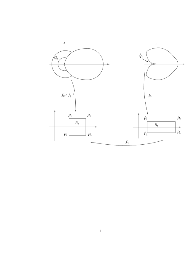
Figure 2. The construction $f^{-1}_{3}\circ f^{-1}_{4}\circ f_{2}\circ f^{-1}_{1}:Q_{t}\rightarrow\tilde{Q}_{t}$

Let

$$\tilde{Q}_{t}=\{(x,y)\in\mathbb{R}^{2}:x\in[-t^{2},-(t/2)^{2}],\ |y|\leq|x|^{s}\}.$$

Define

$$f_{3}(u,v)=\left(-u,\frac{t^{2s}}{(-u)^{s}}v\right)\qquad\forall(u,v)\in\tilde{Q}_{t}.$$

Then $f_{3}$ is diffeomorphic and

(4.1.13) $$Df_{3}(u,v)=\begin{bmatrix}-1&0\\ \frac{st^{2s}}{(-u)^{s+1}}v&\frac{t^{2s}}{(-u)^{s}}\end{bmatrix}.$$

From (4.1.13) we have that

(4.1.14) $$|Df_{3}|\lesssim 1\mbox{ and }J_{f_{3}}\approx-1\qquad\forall(u,v)\in\tilde{Q}_{t}.$$

Analogously to (4.1.10), we have that

(4.1.15) $$K_{f_{3}}(u,v)\approx 1\qquad\forall t\ll 1\mbox{ and }\forall(u,v)\in\tilde{Q}_{t}.$$

Let $\tilde{R}_{t}=f_{3}(\tilde{Q}_{t}).$ Then $\tilde{R}_{t}=[(t/2)^{2},t^{2}]\times[-t^{2s},t^{2s}].$ The same reasons as for (4.1.11) and (4.1.12) imply that

(4.1.16) $$|Df^{-1}_{3}(x,y)|\lesssim 1,\ J_{f^{-1}_{3}}(x,y)\approx-1\mbox{ and }K_{f^{-1}_{3}}(x,y)\approx 1$$

for all $t\ll 1$ and $(x,y)\in\tilde{R}_{t}.$

Denote by $P_{1},P_{2},P_{3},P_{4}$ and $\tilde{P}_{1},\tilde{P}_{2},\tilde{P}_{3},\tilde{P}_{4}$ the four vertices of $\tilde{R}_{t}$ and $R_{t},$ respectively. Then

$$P_{1}=(L^{1}_{t},\frac{\sigma_{t}}{2}),\ P_{2}=(L^{2}_{t},\frac{\sigma_{t}}{2}),\ P_{3}=(L^{2}_{t},-\frac{\sigma_{t}}{2}),\ P_{4}=(L^{1}_{t},-\frac{\sigma_{t}}{2})$$

and

$$\tilde{P}_{1}=((t/2)^{2},t^{2s}),\ \tilde{P}_{2}=(t^{2},t^{2s}),\ \tilde{P}_{3}=(t^{2},-t^{2s}),\ \tilde{P}_{4}=((t/2)^{2},-t^{2s}).$$

Since $\partial M_{s}$ is mapped onto $\partial\Delta_{s}$ by $z^{2},$ the line segment $\tilde{P}_{1}\tilde{P}_{2}$ is mapped onto $P_{1}P_{2}$ by

$$(u,t^{2s})\mapsto\left(\eta(u),\frac{\sigma_{t}}{2}\right)\qquad\forall u\in[(t/2)^{2},t^{2}],$$

and the line segment $\tilde{P}_{4}\tilde{P}_{3}$ is mapped onto $P_{4}P_{3}$ by

$$(u,-t^{2s})\mapsto\left(\eta(u),-\frac{\sigma_{t}}{2}\right)\qquad\forall u\in[(t/2)^{2},t^{2}].$$

Define

(4.1.17) $$f_{4}(u,v)=\left(\eta(u),\frac{\sigma_{t}}{2t^{2s}}v\right)\qquad\forall(u,v)\in\tilde{R}_{t}.$$

Then $f_{4}$ is a diffeomorphism from $\tilde{R}_{t}$ onto $R_{t}$ and

(4.1.18) $$Df_{4}(u,v)=\begin{bmatrix}\eta^{\prime}(u)&0\\ 0&\frac{\sigma_{t}}{2t^{2s}}\end{bmatrix}.$$

By (4.1.2) and (4.1.3) we have that $\eta^{\prime}(u)\approx t^{-1}$ and $\frac{\sigma_{t}}{2t^{2s}}\approx t^{1-2s}$ whenever $t\ll 1$ and $(u,v)\in\tilde{R}_{t}.$ It follows from (4.1.18) that

(4.1.19) $$|Df_{4}(u,v)|\approx t^{1-2s}\mbox{ and }J_{f_{4}}(u,v)\approx t^{-2s}$$

for all $t\ll 1$ and all $(u,v)\in\tilde{R}_{t}.$ Then

(4.1.20) $$K_{f_{4}}(u,v)=\frac{|Df_{4}(u,v)|^{2}}{J_{f_{4}}(u,v)}\approx t^{2-2s}\qquad\forall t\ll 1\mbox{ and }(u,v)\in\tilde{R}_{t}.$$

The same reasons as for (4.1.11) and (4.1.12) imply that

(4.1.21) $$|Df^{-1}_{4}(x,y)|\approx t,\ J_{f^{-1}_{4}}(x,y)\approx t^{2s}\mbox{ and }K_{f^{-1}_{4}}(x,y)\approx t^{2-2s}$$

for all $t\ll 1$ and all $(x,y)\in R_{t}.$

Define

$$F_{t}=f^{-1}_{3}\circ f^{-1}_{4}\circ f_{2}\circ f^{-1}_{1}.$$

Then $F_{t}$ is a diffeomorphism from $Q_{t}$ onto $\tilde{Q}_{t}.$ Therefore

$$DF_{t}(z)=Df^{-1}_{3}(f^{-1}_{4}\circ f_{2}\circ f^{-1}_{1}(z))Df^{-1}_{4}(f_{2}\circ f^{-1}_{1}(z))D(f_{2}\circ f^{-1}_{1})(z)$$

for all $z\in Q_{t}.$ From (4.1.16), (4.1.21) and (4.1.11) it then follows that

$$\int_{Q_{t}}|DF_{t}|^{p}\,dz\leq \int_{Q_{t}}|Df^{-1}_{3}(f^{-1}_{4}\circ f_{2}\circ f^{-1}_{1})|^{p}|Df^{-1}_{4}(f_{2}\circ f^{-1}_{1})|^{p}|Df_{2}\circ f^{-1}_{1}|^{p}\,dz$$

(4.1.22) $$\lesssim t^{p}\mathcal{L}^{2}(Q_{t})\approx t^{2+p}$$

for any $p\geq 0.$ By Lemma 2.1 we have that

$$\int_{Q_{t}}|J_{F_{t}}(z)|\,dz= \int_{Q_{t}}|J_{f^{-1}_{3}}(f^{-1}_{4}\circ f_{2}\circ f^{-1}_{1}(z))||J_{f^{-1}_{4}}(f_{2}\circ f^{-1}_{1}(z))||J_{f_{2}\circ f^{-1}_{1}}(z)|\,dz$$

$$\leq \int_{f_{2}\circ f^{-1}_{1}(Q_{t})}|J_{f^{-1}_{3}}(f^{-1}_{4})||J_{f^{-1}_{4}}|$$

(4.1.23) $$\leq \int_{f^{-1}_{4}\circ f_{2}\circ f^{-1}_{1}(Q_{t})}|J_{f^{-1}_{3}}|\leq\mathcal{L}^{2}(\tilde{Q}_{t}).$$

For a fixed large $j_{0},$ we now consider the set $Q_{t}$ with $t=2^{-j}$ for all $j\geq j_{0}.$ Define

(4.1.24) $$E_{1}=\sum_{j=j_{0}}^{+\infty}F_{2^{-j}}\chi_{Q_{2^{-j}}}.$$

Denote $\Omega_{1}=\cup_{j=j_{0}}^{+\infty}Q_{2^{-j}}\mbox{ and }\tilde{\Omega}_{1}=\cup_{j=j_{0}}^{+\infty}\tilde{Q}_{2^{-j}}.$ Then $E_{1}$ is a homeomorphism from $\Omega_{1}$ onto $\tilde{\Omega}_{1},$ and satisfies (2.2.1) for $E_{1}$ on $\mathcal{L}^{2}$-a.e. $\Omega_{1}.$ In order to prove that $E_{1}$ has finite distortion on $\Omega_{1},$ it thus suffices to prove that $E_{1}\in W^{1,1}_{\text{loc}}(\Omega_{1})$ and $J_{E_{1}}\in L^{1}_{\text{loc}}(\Omega_{1}).$ Actually, from (4.1) and (4.1) we have that

(4.1.25) $$\int_{\Omega_{1}}|DE_{1}|^{p}=\sum_{j=j_{0}}^{+\infty}\int_{Q_{2^{-j}}}|DF_{2^{-j}}(z)|^{p}\,dz\lesssim\sum_{j=j_{0}}^{+\infty}2^{-j(2+p)}<\infty$$

and

(4.1.26) $$\int_{\Omega_{1}}|J_{E_{1}}|=\sum_{j=j_{0}}^{\infty}\int_{Q_{2^{-j}}}|J_{F_{2^{-j}}}|\leq\sum_{j=j_{0}}^{\infty}\mathcal{L}^{2}(\tilde{Q}_{2^{-j}})=\mathcal{L}^{2}(\tilde{\Omega}_{1})<\infty$$

for all $p\geq 1.$

Denote

$$\Omega_{2}=M_{s}^{c}\setminus\Omega_{1}\mbox{ and }\tilde{\Omega}_{2}=\Delta_{s}^{c}\setminus\tilde{\Omega}_{1}.$$

Notice that both $\partial\Omega_{2}$ and $\partial\tilde{\Omega}_{2}$ are piecewise smooth Jordan curves with non-zero angles at the two corners. Therefore both $\partial\Omega_{2}$ and $\partial\tilde{\Omega}_{2}$ are chord-arc curves. By [7] there are bi-Lipschitz mappings

(4.1.27) $$H_{1}:\mathbb{R}^{2}\rightarrow\mathbb{R}^{2}\mbox{ and }H_{2}:\mathbb{R}^{2}\rightarrow\mathbb{R}^{2}$$

such that $H_{1}(\mathbb{S}^{1})=\partial\Omega_{2}$ and $H_{2}(\mathbb{S}^{1})=\partial\tilde{\Omega}_{2}.$ Define

$$h(z)=\begin{cases}E_{1}(z)&\forall z\in\partial\Omega_{2}\cap\partial\Omega_{1},\\ z^{2}&\forall z\in\partial\Omega_{2}\cap\partial M_{s}.\end{cases}$$

Then $h$ is a bi-Lipschitz mapping in terms of the arc lengths. By the chord-arc properties of both $\partial\Omega_{2}$ and $\partial\tilde{\Omega}_{2},$ we have that $h$ is also a bi-Lipschitz mapping with respect to the Euclidean distances. Taking (4.1.27) into account, we conclude that $H^{-1}_{2}\circ h\circ H_{1}:\mathbb{S}^{1}\rightarrow\mathbb{S}^{1}$ is a bi-Lipschitz mapping. By [13, Theorem A] there is then a bi-Lipschitz mapping

(4.1.28) $$H:\mathbb{R}^{2}\rightarrow\mathbb{R}^{2}$$

such that $H|_{\mathbb{S}^{1}}=H^{-1}_{2}\circ h\circ H_{1}.$ Define

(4.1.29) $$E_{2}=H_{2}\circ H\circ H^{-1}_{1}.$$

By (4.1.27) and (4.1.28), we have that $E_{2}$ is a bi-Lipschitz extension of $h.$ Furthermore since $\deg_{M_{s}}(h,w)=1,$ we obtain that $E_{2}$ is orientation-preserving. Hence $E_{2}$ is a quasiconformal mapping. The same reasons as for (2.3.13) and (2.3.14) imply

(4.1.30) $$|DE_{2}(z)|,\ K_{E_{2}}(z)\mbox{ and }J_{E_{2}}(z)\mbox{ are bounded from both above and below}$$

for $\mathcal{L}^{2}$-a.e. $z\in\mathbb{R}^{2},$ and

(4.1.31) $$|DE^{-1}_{2}(w)|,\ K^{-1}_{E_{2}}(w)\mbox{ and }J^{-1}_{E_{2}}(w)\mbox{ are bounded from both above and below}$$

for $\mathcal{L}^{2}$-a.e. $w\in\mathbb{R}^{2}.$

Via (4.1.24) and (4.1.29), we define

(4.1.32) $$E(x,y)=\begin{cases}E_{1}(x,y)&\mbox{ for all }(x,y)\in\Omega_{1},\\ E_{2}(x,y)&\mbox{ for all }(x,y)\in\Omega_{2},\\ (x^{2}-y^{2},2xy)&\mbox{ for all }(x,y)\in\overline{M_{s}}.\end{cases}$$

By the properties of $E_{1}$ and $E_{2},$ we conclude that $E\in\mathcal{E}_{s}.$ ∎

4.2. (1.0.7), (1.0.10) and (1.0.11)

Proof of (1.0.7).

Let $g:\mathbb{D}\rightarrow\Delta_{s}$ be conformal, where $\Delta_{s}$ is defined in (2.3.2) with $s>1.$ In order to prove (1.0.7), it is enough to construct $f\in\mathcal{F}_{s}(g)$ such that $f\in W^{1,p}_{\text{loc}}(\mathbb{R}^{2},{\mathbb{R}}^{2})$ for all $p\geq 1.$ let $E$ be as in (4.1.32). Then $E\in\mathcal{E}_{s}.$ By (4.1.25), (4.1.30) and the fact that $E(z)=z^{2}$ for all $z\in M_{s},$ we obtain that $E\in W^{1,p}_{\text{loc}}(\mathbb{R}^{2},{\mathbb{R}}^{2})$ for all $p\geq 1.$ Let $G_{s}$ be as in (2.3.6) and $\mathfrak{M}_{s}$ be as in (3.0.30). By Lemma 2.6 and the analogous arguments as for (3), we can define $f=E\circ G_{s}\circ\mathfrak{M}_{s}.$ ∎

Proof of (1.0.10).

Let $g:\mathbb{D}\rightarrow\Delta_{s}$ be conformal, where $\Delta_{s}$ is defined in (2.3.2) with $s>1.$ In order to prove (1.0.10), by Lemma 3.5 ($1$) it is enough to construct a mapping $f\in\mathcal{F}_{s}(g)$ such that $f^{-1}\in W^{1,p}_{\text{loc}}(\mathbb{R}^{2},{\mathbb{R}}^{2})$ for all $p<2(s+1)/(2s-1).$ Let $G_{s}$ be as in (2.3.6) and $\mathfrak{M}_{s}$ be defined in (3.0.30). If there is a mapping $E\in\mathcal{E}_{s}$ such that $E^{-1}\in W^{1,p}_{\text{loc}}(\mathbb{R}^{2},{\mathbb{R}}^{2})$ for all $p<2(s+1)/(2s-1),$ by Lemma 2.6 and analogous arguments as for (3.0.32) we can define $f=E\circ G_{s}\circ\mathfrak{M}_{s}.$

Let $E$ be as in (4.1.32). Then $E\in\mathcal{E}_{s}.$ By (4.1.14), (4.1.19) and (4.1.9) we have that

$$|DF^{-1}_{2^{-j}}(w)|\leq|Df_{1}\circ f^{-1}_{2}(f_{4}\circ f_{3}(w))||Df_{4}(f_{3}(w))||Df_{3}(w)|\lesssim 2^{j(2s-1)}$$

for all $j\geq j_{0}$ and $\mathcal{L}^{2}$-a.e. $w\in\tilde{Q}_{2^{-j}}.$ Together with $\mathcal{L}^{2}(\tilde{Q}_{2^{-j}})\approx 2^{-2j(s+1)},$ we hence obtain that

(4.2.1) $$\int_{\tilde{\Omega}_{1}}|DE^{-1}_{1}|^{p}=\sum_{j=j_{0}}^{+\infty}\int_{\tilde{Q}_{2^{-j}}}|DF^{-1}_{2^{-j}}|^{p}\lesssim\sum_{j=j_{0}}^{+\infty}2^{-j(2(s+1)+p(1-2s))}<\infty$$

for all $p<2(s+1)/(2s-1).$ Since

(4.2.2) $$|DE^{-1}(u,v)|\lesssim(u^{2}+v^{2})^{-1/4}\qquad\forall(u,v)\in\Delta_{s},$$

by a change of variables we have that

(4.2.3) $$\int_{\Delta_{s}}|DE^{-1}(w)|^{p}\,dw\lesssim\int_{0}^{2\pi}\int_{0}^{1}r^{1-\frac{p}{2}}\,dr\,d\theta\approx\int_{0}^{1}r^{1-\frac{p}{2}}\,dr<\infty$$

for all $p<2(s+1)/(2s-1).$ By (4.1.31), (4.2.1) and (4.2.3), we conclude that $E^{-1}\in W^{1,p}_{\text{loc}}(\mathbb{R}^{2},{\mathbb{R}}^{2})$ for all $p<2(s+1)/(2s-1).$ ∎

Proof of (1.0.11).

Let $g:\mathbb{D}\rightarrow\Delta_{s}$ be conformal, where $\Delta_{s}$ is defined in (2.3.2) with $s>1.$ In order to prove (1.0.11), by Lemma 3.5 ($2$) it is enough to construct a mapping $f\in\mathcal{F}_{s}(g)$ such that $K_{f^{-1}}\in L^{q}_{\text{loc}}(\mathbb{R}^{2})$ for all $q<(s+1)/(s-1).$ Let $G_{s}$ be as in (2.3.6) and $\mathfrak{M}_{s}$ be as in (3.0.30). If there is a mapping $E\in\mathcal{E}_{s}$ such that $K_{E^{-1}}\in L^{q}_{\text{loc}}(\mathbb{R}^{2})$ for all $q<(s+1)/(s-1),$ by Lemma 2.6 and analogous argument as for (3.0.34) we can define $f=E\circ G_{s}\circ\mathfrak{M}_{s}.$

Let $E$ be as in (4.1.32). Then $E\in\mathcal{E}_{s}.$ From (4.1.10), (4.1.20) and (4.1.15), we have that

$$K_{F^{-1}_{2^{-j}}}(w)=K_{f_{1}\circ f^{-1}_{2}}(f_{4}\circ f_{3}(w))K_{f_{4}}(f_{3}(w))K_{f_{3}}(w)\approx 2^{j(2s-2)}$$

for all $j\geq j_{0}$ and $\mathcal{L}^{2}$-a.e. $w\in\tilde{Q}_{2^{-j}}.$ Together with $\mathcal{L}^{2}(\tilde{Q}_{2^{-j}})\approx 2^{-j2(s+1)},$ we then obtain that

(4.2.4) $$\int_{\tilde{\Omega}_{1}}K^{q}_{E^{-1}}=\sum_{j=j_{0}}^{+\infty}\int_{\tilde{Q}_{2^{-j}}}K^{q}_{F^{-1}_{2^{-j}}}\lesssim\sum_{j=j_{0}}^{+\infty}2^{2j[(s-1)q-(s+1)]}<\infty$$

for all $q<(s+1)/(s-1).$ By (4.1.31), (4.2.4) and the fact that $E$ is conformal on $M_{s},$ we conclude that $K_{E^{-1}}\in L^{q}_{\text{loc}}(\mathbb{R}^{2})$ for all $q<(s+1)/(s-1).$

∎

4.3. (1.0.8)

Proof.

Let $g:\mathbb{D}\rightarrow\Delta_{s}$ be conformal, where $\Delta_{s}$ is defined as (2.3.2) with $s>1.$ In order to prove (1.0.8), via Lemma 3.5 ($3$) it is enough to construct a mapping $f\in\mathcal{F}_{s}(g)$ such that $K_{f}\in L^{q}_{\text{loc}}$ for all $q<\max\{1,1/(s-1)\}.$ Let $G_{s}$ be as in (2.3.6) and $\mathfrak{M}_{s}$ be as in (3.0.30). If $E\in\mathcal{E}_{s}$ such that $K_{E}\in L^{q}_{\text{loc}}$ for all $q<\max\{1,1/(s-1)\},$ by Lemma 2.6 and analogous arguments as for (3) we can define $f=E\circ G_{s}\circ\mathfrak{M}_{s}.$

Let $E$ be as in (4.1.32). Then $E\in\mathcal{E}_{s}.$ From (4.1.16), (4.1.21) and (4.1.12), it follows that

$$K_{F_{2^{-j}}}(z)=K_{f^{-1}_{3}}(f^{-1}_{4}\circ f_{2}\circ f^{-1}_{1}(z))K_{f^{-1}_{4}}(f_{2}\circ f^{-1}_{1}(z))K_{f_{2}\circ f^{-1}_{1}}(z)\approx 2^{2j(s-1)}$$

for all $j\geq j_{0}$ and $\mathcal{L}^{2}$-a.e. $z\in Q_{2^{-j}}.$ Together with $\mathcal{L}^{2}(Q_{2^{-j}})\approx 2^{-2j}$ we then have that

(4.3.1) $$\int_{\Omega_{1}}K^{q}_{E}=\sum_{j=j_{0}}^{+\infty}\int_{Q_{2^{-j}}}K^{q}_{F_{2^{-j}}}\approx\sum_{j=j_{0}}^{+\infty}2^{2j(q(s-1)-1)}<\infty$$

for all $q<1/(s-1).$ By (4.3.1), (4.1.30) and the fact that $E$ is conformal on $M_{s},$ we conclude that $K_{E}\in L^{q}_{\text{loc}}(\mathbb{R}^{2})$ for all $q<1/(s-1).$ Therefore we have proved (1.0.8) whenever $s\in(1,2).$

We next consider the case $s\in[2,\infty).$ It is enough to construct a mapping $E\in\mathcal{E}_{s}$ such that $K_{E}\in L^{q}_{\text{loc}}$ for all $q<1.$ Except for redefining $f^{-1}_{4}:R_{t}\rightarrow\tilde{R}_{t}$ as in (4.1.17), we follow all processes in Section 4.1 to define a new $E,$ see FIGURE 3. Let $\alpha_{t}$ and $\beta_{t}$ be the length of sides of $\tilde{R}_{t},$ and $\gamma_{t}$ be the length of a side of $R_{t}.$ Whenever $t\ll 1,$ we have that

(4.3.2) $$\alpha_{t}=t^{2}-(t/2)^{2}\approx t^{2},\ \beta_{t}=2t^{2s}\mbox{ and }\gamma_{t}=\eta(t^{2})-\eta((t/2)^{2})\approx t.$$

Let $\tilde{T}_{0}=\tilde{Q}_{1}\tilde{Q}_{2}\tilde{Q}_{3}\tilde{Q}_{4}$ be the concentric square of $\tilde{R}_{t}$ with side length $\beta_{t}/2.$ Set

(4.3.3) $$\delta_{t}=\exp(-t^{-1})\qquad\mbox{for }t>0$$

and let $T_{0}=Q_{1}Q_{2}Q_{3}Q_{4}$ be the concentric square of $R_{t}$ with side length $\gamma_{t}(1-2\delta_{t}).$ We divide $R_{t}\setminus T_{0}$ into four isosceles trapezoids $T_{1},\ T_{2},\ T_{3}$ and $T_{4}.$ Similarly, we obtain isosceles trapezoids $\tilde{T}_{1},\ \tilde{T}_{2},\ \tilde{T}_{3},\ \tilde{T}_{4}$ from $\tilde{R}_{t}\setminus\tilde{T}_{0},$ see FIGURE 3.

Figure 3. The redefined $f^{-1}_{4}:R_{t}\rightarrow\tilde{R}_{t}$

We first define a diffeomorphism from $T_{1}$ onto $\tilde{T}_{1}.$ Define

(4.3.4) $$A_{2}(x,y)=\frac{\beta_{t}}{4\delta_{t}\gamma_{t}}\left(y-\gamma_{t}\big{(}\frac{1}{2}-\delta_{t}\big{)}\right)+\frac{\beta_{t}}{4}\qquad\forall(x,y)\in T_{1}.$$

For a given $(x,y)\in T_{1},$ let $(x_{p},y)=P_{1}Q_{1}\cap\{(X,Y)\in\mathbb{R}^{2}:Y=y\}$, $(\tilde{x}_{p},A_{2})=\tilde{P}_{1}\tilde{Q}_{1}\cap\{(X,Y)\in\mathbb{R}^{2}:Y=A_{2}(x,y)\}$, $\ell(y)$ be the length of $T_{1}\cap\{(X,Y):Y=y\},$ and $\tilde{\ell}(y)$ be the length of $\tilde{T}_{1}\cap\{(X,Y):Y=A_{2}\}.$ Denote $(P_{1})_{1}$ by the first coordinate of $P_{1}.$ Then

(4.3.5) $$x_{p}=-y+\frac{\gamma_{t}}{2}+(P_{1})_{1}\mbox{ and }\tilde{x}_{p}=\frac{2\alpha_{t}-\beta_{t}}{\beta_{t}}\left(\frac{\beta_{t}}{2}-A_{2}\right)+(\tilde{P}_{1})_{1},$$

(4.3.6) $$\ell(y)=2y\approx\gamma_{t}\mbox{ and }\tilde{\ell}(y)=\frac{4\alpha_{t}-2\beta_{t}}{\beta_{t}}A_{2}(x,y)+\beta_{t}-\alpha_{t}\geq\frac{\beta_{t}}{2}.$$

Let $u=\frac{\gamma_{t}}{\ell(y)}(x-x_{p})+(P_{1})_{1}$ for $(x,y)\in T_{1},$ and $\eta$ be as in (4.1.1). Define

(4.3.7) $$A_{1}(x,y)=\frac{\tilde{\ell}(y)}{\alpha_{t}}\left(\eta^{-1}(u)-(\tilde{P}_{1})_{1}\right)+\tilde{x}_{p}\qquad\forall(x,y)\in T_{1}.$$

By (4.3.7) and (4.3.4), we have that

(4.3.8) $$A=(A_{1},A_{2})$$

is a diffeomorphism from $T_{1}$ onto $\tilde{T}_{1}.$ We next give some estimates for $A.$ By (4.3.2) we have that

(4.3.9) $$\frac{\partial A_{2}(x,y)}{\partial y}=\frac{\beta_{t}}{4\delta_{t}\gamma_{t}}\approx\frac{t^{2s-1}}{\delta_{t}}\qquad\forall(x,y)\in T_{1}.$$

From (4.1.2), (4.3.6) and (4.3.2) it follows that

(4.3.10) $$\frac{\partial A_{1}(x,y)}{\partial x}=\frac{\tilde{\ell}(y)}{\alpha_{t}}(\eta^{-1})^{\prime}(u)\frac{\partial u}{\partial x}\approx\frac{\tilde{\ell}(y)}{t}\qquad\forall(x,y)\in T_{1}.$$

Moreover, by (4.3.5) and (4.3.6) we have that

(4.3.11) $$\frac{\partial x_{p}}{\partial y}=-1,\ \frac{\partial\tilde{x}_{p}}{\partial y}=\frac{\beta_{t}-2\alpha_{t}}{\beta_{t}}\frac{\partial A_{2}}{\partial y},\ \frac{\partial\ell(y)}{\partial y}=2\mbox{ and }\frac{\partial\tilde{\ell}(y)}{\partial y}=\frac{4\alpha_{t}-2\beta_{t}}{\beta_{t}}\frac{\partial A_{2}}{\partial y}.$$

It follows from (4.3.11) that

$$\frac{\partial A_{1}}{\partial y}= \frac{\partial\tilde{x}_{p}}{\partial y}+\frac{\partial\tilde{\ell}(y)}{\alpha_{t}\partial y}\left(\eta^{-1}(u)-(\tilde{P}_{1})_{1}\right)+\frac{\tilde{\ell}(y)}{\alpha_{t}}(\eta^{-1})^{\prime}(u)\frac{\partial u}{\partial y}$$

$$= \frac{2\alpha_{t}-\beta_{t}}{\beta_{t}}\frac{\partial A_{2}}{\partial y}\left[-1+\frac{2}{\alpha_{t}}(\eta^{-1}(u)-(\tilde{P}_{1})_{1})\right]$$

(4.3.12) $$+\frac{\gamma_{t}\tilde{\ell}(y)}{\alpha_{t}\ell(y)}(\eta^{-1})^{\prime}(u)\left[1-\frac{2}{\ell(y)}(x-x_{p})\right].$$

Notice that $0\leq\eta^{-1}(u)-(\tilde{P}_{1})_{1}\leq\alpha_{t}$ and $0\leq x-x_{p}\leq\ell(y)$ for all $(x,y)\in T_{1}.$ Therefore (4.3) together with (4.3.2) and (4.3.9) implies

(4.3.13) $$\left|\frac{\partial A_{1}(x,y)}{\partial y}\right|\lesssim\frac{2\alpha_{t}-\beta_{t}}{\beta_{t}}\frac{\partial A_{2}(x,y)}{\partial y}\approx\frac{t}{\delta_{t}}\qquad\forall(x,y)\in T_{1}.$$

We conclude from (4.3.9), (4.3.10) and (4.3.13) that

(4.3.14) $$|DA(x,y)|\lesssim\max\left\{\left|\frac{\partial A_{1}}{\partial x}\right|,\ \left|\frac{\partial A_{1}}{\partial y}\right|,\ \left|\frac{\partial A_{2}}{\partial x}\right|,\ \left|\frac{\partial A_{2}}{\partial y}\right|\right\}\lesssim\frac{t}{\delta_{t}}$$

and

(4.3.15) $$J_{A}(x,y)=\frac{\partial A_{1}}{\partial x}\frac{\partial A_{2}}{\partial y}\approx\frac{t^{2s-2}\tilde{\ell}(y)}{\delta_{t}}$$

for all $t\ll 1$ and all $(x,y)\in T_{1}.$ Moreover by (4.3.14), (4.3.15) and (4.3.6) we have that

(4.3.16) $$K_{A}(x,y)=\frac{|DA(x,y)|^{2}}{J_{A}(x,y)}\lesssim\frac{t^{4-2s}}{\delta_{t}\tilde{\ell}(y)}\lesssim\frac{t^{4(1-s)}}{\delta_{t}}$$

holds for all $t\ll 1$ and all $(x,y)\in T_{1}.$

We next define a diffeomorphism from $T_{2}$ onto $\tilde{T}_{2}.$ Denote by $P_{c}$ and $\tilde{P}_{c}$ be the center of $R_{t}$ and $\tilde{R}_{t},$ respectively. Given $(x,y)\in T_{2},$ we define

$$B_{1}(x,y)=\frac{2\alpha_{t}-\beta_{t}}{4\delta_{t}\gamma_{t}}\left(x-(P_{c})_{1}-\frac{\gamma_{t}}{2}\right)+(\tilde{P}_{c})_{1}+\frac{\alpha_{t}}{2},\ B_{2}(x,y)=y\frac{a(x-(P_{c})_{1})+b}{c(x-(P_{c})_{1})+d},$$

where $a,\ b,\ c,\ d$ satisfy

(4.3.17) $$a\gamma_{t}(\frac{1}{2}-\delta_{t})+b=\frac{\beta_{t}}{4},\ a\frac{\gamma_{t}}{2}+b=\frac{\beta_{t}}{2},\ c\gamma_{t}(\frac{1}{2}-\delta_{t})+d=\gamma_{t}(\frac{1}{2}-\delta_{t}),\ c\frac{\gamma_{t}}{2}+d=\frac{\gamma_{t}}{2}.$$

Then

(4.3.18) $$B=(B_{1},B_{2})$$

is a diffeomorphism from $T_{2}$ onto $\tilde{T}_{2}.$ By (4.3.2) we have that

(4.3.19) $$\frac{\partial B_{1}(x,y)}{\partial x}=\frac{2\alpha_{t}-\beta_{t}}{4\delta_{t}\gamma_{t}}\approx\frac{t}{\delta_{t}}\qquad\forall(x,y)\in T_{2}.$$

Moreover, from (4.3.17) and (4.3.2) we have that

(4.3.20) $$\frac{\partial B_{2}(x,y)}{\partial y}=\frac{a(x-(P_{c})_{1})+b}{c(x-(P_{c})_{1})+d}\approx\frac{\beta_{t}}{\gamma_{t}}\approx t^{2s-1}$$

and

(4.3.21) $$\left|\frac{\partial B_{2}(x,y)}{\partial x}\right|=\frac{|y(ad-bc)|}{[c(x-(P_{c})_{1})+d]^{2}}\lesssim\frac{\gamma_{t}b}{\gamma^{2}_{t}}\approx t^{2s-1}$$

for all $(x,y)\in T_{2}.$ We then conclude from (4.3.19), (4.3.20) and (4.3.21) that

(4.3.22) $$|DB(x,y)|\lesssim\max\left\{\left|\frac{\partial B_{1}}{\partial x}\right|,\ \left|\frac{\partial B_{1}}{\partial y}\right|,\ \left|\frac{\partial B_{2}}{\partial x}\right|,\ \left|\frac{\partial B_{2}}{\partial y}\right|\right\}\lesssim\frac{t}{\delta_{t}}$$

and

(4.3.23) $$J_{B}(x,y)=\frac{\partial B_{1}}{\partial x}\frac{\partial B_{2}}{\partial y}\approx\frac{t^{2s}}{\delta_{t}}.$$

for all $t\ll 1$ and all $(x,y)\in T_{2}.$ Moreover by (4.3.22) and (4.3.23) we have that

(4.3.24) $$K_{B}(x,y)=\frac{|DB(x,y)|^{2}}{J_{B}(x,y)}\lesssim\frac{t^{2(1-s)}}{\delta_{t}}$$

for all $t\ll 1$ and all $(x,y)\in T_{2}.$

We next construct a diffeomorphism $C:T_{0}\rightarrow\tilde{T}_{0}.$ By (4.3.8) and (4.3.18) we have that $Q_{1}Q_{2}$ is mapped onto $\tilde{Q}_{1}\tilde{Q}_{2}$ by $A_{1}(\cdot,\gamma_{t}(1/2-\delta_{t}),$ and $Q_{2}Q_{3}$ is mapped onto $\tilde{Q}_{2}\tilde{Q}_{3}$ by $B_{2}((P_{c})_{1}+\gamma_{t}(1/2-\delta_{t}),\cdot).$ For a given $(x,y)\in T_{0},$ define

(4.3.25) $$C(x,y)=\left(A_{1}\big{(}x,\gamma_{t}(\frac{1}{2}-\delta_{t})\big{)},B_{2}\big{(}(P_{c})_{1}+\gamma_{t}(\frac{1}{2}-\delta_{t}),y\big{)}\right).$$

Then $C:T_{0}\rightarrow\tilde{T}_{0}$ is diffeomorphic. By (4.3.10) and (4.3.20), we have that

$$\frac{\partial}{\partial x}A_{1}(x,\gamma_{t}(1/2-\delta_{t})\approx t^{2s-1},\ \frac{\partial}{y}B_{2}((P_{c})_{1}+\gamma_{t}(1/2-\delta_{t}),y)\approx t^{2s-1}$$

for all $(x,y)\in T_{0}.$ Therefore

(4.3.26) $$|DC(x,y)|\lesssim t^{2s-1}\mbox{ and }K_{C}(x,y)\approx 1$$

for all $t\ll 1$ and all $(x,y)\in T_{0}.$

Via (4.3.8), (4.3.18) and (4.3.25), we redefine $f^{-1}_{4}:R_{t}\rightarrow\tilde{R}_{t}$ in (4.1.17) as

(4.3.27) $$f^{-1}_{4}(x,y)=\begin{cases}A(x,y)&\forall(x,y)\in T_{1},\\ B(x,y)&\forall(x,y)\in T_{2},\\ \left(A_{1}(x,-y),-A_{2}(x,-y)\right),&\forall(x,y)\in T_{3},\\ (2(\tilde{P}_{c})_{1}-B_{1}(2(P_{c})_{1}-x,y),B_{2}(2(P_{c})_{1}-x,y))&\forall(x,y)\in T_{4},\\ C(x,y)&\forall(x,y)\in T_{0}.\end{cases}$$

Like in Section 4.1, by taking a fixed $j_{0}\gg 1$ we then define $F_{2^{-j}}:Q_{2^{-j}}\rightarrow\tilde{Q}_{2^{-j}}$ for all $j\geq j_{0}$, $E_{1}:\Omega_{1}\rightarrow\tilde{\Omega}_{1}$, $E_{2}:\Omega_{2}\rightarrow\tilde{\Omega}_{2}$ and $E:{\mathbb{R}}^{2}\rightarrow{\mathbb{R}}^{2}.$ It is not difficult to see that the new-defined $E$ is a homeomorphism such that $E(z)=z^{2}$ for all $z\in\overline{M_{s}}$ and satisfies (2.2.1) for $E$ on $\mathcal{L}^{2}$-a.e. $\mathbb{R}^{2}.$ To show $E\in\mathcal{E}_{s},$ it is then enough to prove that $E\in W^{1,1}_{\text{loc}}({\mathbb{R}}^{2},{\mathbb{R}}^{2})$ and $J_{E}\in L^{1}_{\text{loc}}({\mathbb{R}}^{2}).$ By (4.1.11), (4.1.16), (4.3.14), (4.3.22) and (4.3.26), we have that

$$DF_{2^{-j}}(z)= Df^{-1}_{3}(f^{-1}_{4}\circ f_{2}\circ f^{-1}_{1}(z))Df^{-1}_{4}(f_{2}\circ f^{-1}_{1}(z))D(f_{2}\circ f^{-1}_{1})(z)$$

(4.3.28) $$\lesssim \begin{cases}\frac{2^{-j}}{\delta_{2^{-j}}}&\mathcal{L}^{2}\mbox{-a.e. }z\in f_{1}\circ f^{-1}_{2}(\cup_{k=1}^{4}T_{k}),\\ 2^{j(1-2s)}&\mathcal{L}^{2}\mbox{-a.e. }z\in f_{1}\circ f^{-1}_{2}(T_{0}),\end{cases}$$

for all $j\geq j_{0}.$ Notice that

$$\mathcal{L}^{2}(T_{0})=(\gamma_{2^{-j}}(1-2\delta_{2^{-j}}))^{2}\approx 2^{-2j},\ \mathcal{L}^{2}(T_{k})=\delta_{2^{-j}}\gamma^{2}_{2^{-j}}(1-\delta_{2^{-j}})\approx\delta_{2^{-j}}2^{-2j}$$

for all $k=1,2,3,4$ and all $j\geq j_{0}.$ It hence follows from (4.1.9) that

(4.3.29) $$\mathcal{L}^{2}(f_{1}\circ f^{-1}_{2}(T_{0}))\approx 2^{-2j},\ \mathcal{L}^{2}(f_{1}\circ f^{-1}_{2}(T_{k}))\approx\delta_{2^{-j}}2^{-2j}\quad\mbox{for all }k=1,2,3,4.$$

By (4.3) and (4.3.29) we then have that

$$\int_{Q_{2^{-j}}}|DF_{2^{-j}}|=\sum_{k=0}^{4}\int_{f_{1}\circ f^{-1}_{2}(T_{k})}|DF_{2^{-j}}|\lesssim 2^{-3j}+2^{-j(2s+1)}\lesssim 2^{-3j}\qquad\forall j\geq j_{0}.$$

Therefore

(4.3.30) $$\int_{\Omega_{1}}|DE_{1}|=\sum_{j=j_{0}}^{\infty}\int_{Q_{2^{-j}}}|DF_{2^{-j}}|\lesssim\sum_{j=j_{0}}^{\infty}2^{-3j}<\infty.$$

By (4.1.30), (4.3.30) and the fact that $E(z)=z^{2}$ for all $z\in M_{s},$ we have that $E\in W^{1,1}_{\text{loc}}(\mathbb{R}^{2},{\mathbb{R}}^{2}).$ Analogously to (4.1.26), we have that

(4.3.31) $$\int_{\Omega_{1}}|J_{E_{1}}|\leq\mathcal{L}^{2}(\tilde{\Omega}_{1})<\infty.$$

From (4.1.30), (4.3.31) and the fact that $E(z)=z^{2}$ for all $z\in M_{s},$ we have that $J_{E}\in L^{1}_{\text{loc}}(\mathbb{R}^{2}).$

We next show $K_{E}\in L^{q}_{\text{loc}}(\mathbb{R}^{2})$ for all $q<1.$ By (4.1.12), (4.1.16), (4.3.16), (4.3.24) and (4.3.26), we have that

(4.3.32) $$K_{F_{2^{-j}}}(z)\lesssim\begin{cases}\frac{2^{4j(s-1)}}{\delta_{2^{-j}}}&\forall\ z\in f_{1}\circ f^{-1}_{2}(T_{1}\cup T_{3}),\\ \frac{2^{2j(s-1)}}{\delta_{2^{-j}}}&\forall\ z\in f_{1}\circ f^{-1}_{2}(T_{2}\cup T_{4}),\\ 1&\forall\ z\in f_{1}\circ f^{-1}_{2}(T_{0}).\end{cases}$$

for all $j\geq j_{0}.$ For any $q\geq 0,$ via (4.3.29) and (4.3.32) we obtain that

$$\int_{Q_{2^{-j}}}K^{q}_{F_{2^{-j}}}=\sum_{k=0}^{4}\int_{f_{1}\circ f^{-1}_{2}(T_{k})}K^{q}_{F_{2^{-j}}}\lesssim\delta^{1-q}_{2^{-j}}2^{j(4q(s-1)-2)}(1+2^{2qj(1-s)})+2^{-2j}$$

for all $j\geq j_{0}.$ Therefore

$$\int_{\Omega_{1}}K^{q}_{E}= \sum_{j=j_{0}}^{+\infty}\int_{Q_{2^{-j}}}K^{q}_{F_{2^{-j}}}$$

(4.3.33) $$\lesssim \sum_{j=j_{0}}^{+\infty}\exp((q-1)2^{j})2^{j(4q(s-1)-2)}(1+2^{j2q(1-s)})+\sum_{j=j_{0}}^{+\infty}2^{-2j}<+\infty$$

for all $q\in(0,1)$ and each $s>1.$ By (4.1.30), (4.3) and the fact that $E$ is conformal on $M_{s},$ we conclude that $K_{E}\in L^{q}_{\text{loc}}({\mathbb{R}}^{2})$ for all $q\in(0,1).$ ∎

4.4. (1.2)

Proof of (1.2).

Let $g:\mathbb{D}\rightarrow\Delta_{s}$ be conformal, where $\Delta_{s}$ is defined in (2.3.2) with $s>1.$ In order to prove (1.2), via Lemma 3.5 ($4$) it is enough to construct $f\in\mathcal{F}_{s}(g)$ such that $f\in W^{1,p}_{\text{loc}}(\mathbb{R}^{2},{\mathbb{R}}^{2})$ for some $p>1$ and $K_{f}\in L^{q}_{\text{loc}}$ for all $q<\max\{1/(s-1),3p/((2s-1)p+4-2s)\}.$

We consider the case $s\in(1,2]$ first. Let $G_{s}$ be as in (2.3.6) and $\mathfrak{M}_{s}$ be as in (3.0.30). If $E\in\mathcal{E}_{s}$ satisfying that $E\in W^{1,p}_{\text{loc}}(\mathbb{R}^{2},{\mathbb{R}}^{2})$ for some $p>1$ and $K_{E}\in L^{q}_{\text{loc}}$ for all $q<1/(s-1),$ by Lemma 2.6 and the analogous arguments as for (3) and (3), we can define $f=E\circ G_{s}\circ\mathfrak{M}_{s}.$ We now let $E$ be as in (4.1.32). Then $E\in\mathcal{E}_{s}.$ By (4.1.25), (4.1.30) and the fact that $E(z)=z^{2}$ for all $z\in M_{s},$ we obtain that $E\in W^{1,p}_{\text{loc}}(\mathbb{R}^{2},{\mathbb{R}}^{2})$ for all $p\geq 1.$ From (4.1.16), (4.1.21) and (4.1.12), it follows that

$$K_{F_{2^{-j}}}(z)=K_{f^{-1}_{3}}(f^{-1}_{4}\circ f_{2}\circ f^{-1}_{1}(z))K_{f^{-1}_{4}}(f_{2}\circ f^{-1}_{1}(z))K_{f_{2}\circ f^{-1}_{1}}(z)\approx 2^{(2s-2)j}$$

for all $j\geq j_{0}$ and $\mathcal{L}^{2}$-a.e. $z\in Q_{2^{-j}}.$ Together with $\mathcal{L}^{2}(Q_{2^{-j}})\approx 2^{-2j},$ we then obtain

(4.4.1) $$\int_{\Omega_{1}}K^{q}_{E}=\sum_{j=j_{0}}^{+\infty}\int_{Q_{2^{-j}}}K^{q}_{F_{2^{-j}}}\approx\sum_{j=j_{0}}^{+\infty}2^{-j2(1+q(1-s))}<\infty$$

for all $q<1/(s-1).$ By (4.4.1), (4.1.30) and the fact that $E$ is conformal on $M_{s},$ we have that $K_{E}\in L^{q}_{\text{loc}}(\mathbb{R}^{2})$ for all $q<1/(s-1).$

We turn to the case $s>2.$ Let $M(p,s)=3p/((2s-1)p+4-2s)$ with $p>1.$ Analogously to the case $s\in(1,2],$ it is enough to construct $E\in\mathcal{E}_{s}$ such that $E\in W^{1,p}_{\text{loc}}(\mathbb{R}^{2},{\mathbb{R}}^{2})$ and $K_{E}\in L^{q}_{\text{loc}}(\mathbb{R}^{2})$ for all $q\in(0,M(p,s)).$ Redefining $\delta_{t}$ in (4.3.3) as $\delta_{t}=t^{\frac{p+2}{p-1}}\log^{\frac{p}{p-1}}(t^{-1}).$ We follow the methods in Section 4.3 to define a new $f^{-1}_{4}.$ Set $j_{0}\gg 1.$ There are then new $F_{2^{-j}}:Q_{2^{-j}}\rightarrow\tilde{Q}_{2^{-j}}$ for all $j\geq j_{0}$, $E_{1}:\Omega_{1}\rightarrow\tilde{\Omega}_{1}$, $E_{2}:\Omega_{2}\rightarrow\tilde{\Omega}_{2}$ and $E:{\mathbb{R}}^{2}\rightarrow{\mathbb{R}}^{2}.$ It is not difficult to see that the new $E$ is homeomorphic, satisfies (2.2.1) for $E$ on $\mathcal{L}^{2}$-a.e. $\mathbb{R}^{2}$ and $J_{E}\in L^{1}_{\text{loc}}(\mathbb{R}^{2}).$ To show that $E$ satisfies all requirements, it is enough to check that $E\in W^{1,p}_{\text{loc}}(\mathbb{R}^{2},{\mathbb{R}}^{2})$ and $K_{E}\in L^{q}_{\text{loc}}(\mathbb{R}^{2})$ for all $q\in(0,M(p,s)).$

From (4.1.11), (4.1.16), (4.3.14), (4.3.22) and (4.3.26) we have that

(4.4.2) $$|DF_{2^{-j}}(z)|\lesssim\begin{cases}\frac{2^{-j}}{\delta_{2^{-j}}}&\forall z\in f_{1}\circ f^{-1}_{2}(\cup_{k=1}^{4}T_{k}),\\ 2^{j(1-2s)}&\forall z\in f_{1}\circ f^{-1}_{2}(T_{0}),\end{cases}$$

for all $j\geq j_{0}.$ It follows from (4.4.2) and (4.3.29) that

$$\int_{Q_{2^{-j}}}|DF_{2^{-j}}|^{p}=\sum_{k=0}^{4}\int_{f_{1}\circ f^{-1}_{2}(T_{k})}|DF_{2^{-j}}|^{p}\lesssim\delta^{1-p}_{2^{-j}}2^{-j(2+p)}+2^{j(p(1-2s)-2)}.$$

Therefore

(4.4.3) $$\int_{\Omega_{1}}|DE|^{p}=\sum_{j=j_{0}}^{+\infty}\int_{Q_{2^{-j}}}|DF_{2^{-j}}|^{p}\lesssim\sum_{j=j_{0}}^{+\infty}\frac{1}{j^{p}}+\sum_{j=j_{0}}^{+\infty}2^{-j(p(2s-1)+2)}<\infty.$$

By (4.4.3), (4.1.30) and the fact that $E(z)=z^{2}$ for all $z\in M_{s},$ we conclude that $E\in W^{1,p}_{\text{loc}}(\mathbb{R}^{2},{\mathbb{R}}^{2}).$ By (4.1.11), (4.1.12), Lemma 2.1 and (4.1.16), we have

$$\int_{f_{1}\circ f^{-1}_{2}(T_{1})}K^{q}_{F_{2^{-j}}}\approx \int_{f_{1}\circ f^{-1}_{2}(T_{1})}K^{q}_{f^{-1}_{3}}(f^{-1}_{4}\circ f_{2}\circ f^{-1}_{1})K^{q}_{f^{-1}_{4}}(f_{2}\circ f^{-1}_{1})K^{q}_{f_{2}\circ f^{-1}_{1}}\big{|}J_{f_{2}\circ f^{-1}_{1}}\big{|}$$

$$\leq \int_{T_{1}}K^{q}_{f^{-1}_{3}}(f^{-1}_{4})K^{q}_{f^{-1}_{4}}$$

(4.4.4) $$\lesssim \int_{T_{1}}K^{q}_{f^{-1}_{4}}$$

for all $q\geq 0$ and all $j\geq j_{0}.$ Notice $\tilde{\ell}(\gamma_{2^{-j}}/2)=\alpha_{2^{-j}}$ and $\tilde{\ell}(\gamma_{2^{-j}}(\frac{1}{2}-\delta_{2^{-j}}))=\beta_{2^{-j}}/2$ for all $j\geq 1.$ By Fubini’s theorem, (4.3.16), (4.3.6) and (4.3.2) we then have

$$\int_{T_{1}}K^{q}_{f^{-1}_{4}}\lesssim \int_{\gamma_{2^{-j}}(\frac{1}{2}-\delta_{2^{-j}})}^{\frac{\gamma_{2^{-j}}}{2}}\int_{x_{p}}^{x_{p}+\ell(y)}\left(\frac{2^{j(2s-4)}}{\delta_{2^{-j}}\tilde{\ell}(y)}\right)^{q}\,dx\,dy$$

$$\approx \frac{2^{jq(2s-4)}\gamma_{2^{-j}}}{\delta^{q}_{2^{-j}}}\int_{\gamma_{2^{-j}}(\frac{1}{2}-\delta_{2^{-j}})}^{\frac{\gamma_{2^{-j}}}{2}}\frac{1}{\tilde{\ell}^{q}(y)}\,dy$$

$$= \frac{2^{jq(2s-4)}\gamma_{2^{-j}}}{(1-q)\delta^{q}_{2^{-j}}}\frac{2\delta_{2^{-j}}\gamma_{2^{-j}}}{2\alpha_{2^{-j}}-\beta_{2^{-j}}}\left(\tilde{\ell}^{1-q}(\frac{\gamma_{2^{-j}}}{2})-\tilde{\ell}^{1-q}(\gamma_{2^{-j}}(\frac{1}{2}-\delta_{2^{-j}}))\right)$$

(4.4.5) $$\lesssim \frac{\delta^{1-q}_{2^{-j}}2^{-2j[1+q(1-s)]}}{1-M(p,s)}$$

for any fixed $q\in(0,M(p,s)).$ Combining (4.4) with (4.4) implies that

(4.4.6) $$\int_{f_{1}\circ f^{-1}_{2}(T_{1})}K^{q}_{F_{2^{-j}}}\lesssim\delta^{1-q}_{2^{-j}}2^{-2j[1+q(1-s)]}\qquad\forall j\geq j_{0}.$$

By symmetry of $f^{-1}_{4}$ between $T_{1}$ and $T_{3},$ it follows from (4.4.6) that

(4.4.7) $$\int_{f_{1}\circ f^{-1}_{2}(T_{3})}K^{q}_{F_{2^{-j}}}=\int_{f_{1}\circ f^{-1}_{2}(T_{1})}K^{q}_{F_{2^{-j}}}\lesssim\delta^{1-q}_{2^{-j}}2^{-2j[1+q(1-s)]}$$

for all $j\geq j_{0}.$ By (4.3.32) and (4.3.29), we have that

(4.4.8) $$\int_{f_{1}\circ f^{-1}_{2}(T_{0})}K^{q}_{F_{2^{-j}}}\lesssim 2^{-2j}$$

and

(4.4.9) $$\int_{f_{1}\circ f^{-1}_{2}(T_{2}\cup T_{4})}K^{q}_{F_{2^{-j}}}\lesssim\delta_{2^{-j}}2^{-2j}\left(\frac{2^{2j(s-1)}}{\delta_{2^{-j}}}\right)^{q}=\delta^{1-q}_{2^{-j}}2^{2j[q(s-1)-1]}$$

for all $j\geq j_{0}.$ From (4.4.6), (4.4.7), (4.4.8) and (4.4.9), we conclude that

$$\int_{\Omega_{1}}K^{q}_{E}= \sum_{j=j_{0}}^{+\infty}\int_{Q_{2^{-j}}}K^{q}_{F_{2^{-j}}}=\sum_{j=j_{0}}^{+\infty}\sum_{k=0}^{4}\int_{f_{1}\circ f^{-1}_{2}(T_{k})}K^{q}_{F_{2^{-j}}}$$

(4.4.10) $$\lesssim \sum_{j=j_{0}}^{+\infty}2^{-2j}+2^{-j\left(\frac{(p+2)(1-q)}{p-1}+2[1+q(1-s)]\right)}\log^{\frac{p(1-q)}{p-1}}\left(2^{j}\right).$$

Note that

$$\frac{(p+2)(1-q)}{p-1}+2[1+q(1-s)]>0\Leftrightarrow q<M(p,s).$$

It from (4.4) follows that $\int_{\Omega_{1}}K^{q}_{E}<\infty$ for all $q\in(0,M(p,s)).$ Together with (4.1.30) and the fact that $E$ is conformal on $M_{s},$ we conclude that $K_{E}\in L^{q}_{\text{loc}}(\mathbb{R}^{2})$ for all $q\in(0,M(p,s)).$ ∎

5. Proof of Theorem 1.1

Proof.

Let $\Delta$ be as in (1.0.1). The representation of $\partial\Delta$ in Cartesian coordinates is

$$(x^{2}+y^{2})^{2}-4x(x^{2}+y^{2})-4y^{2}=0.$$

Hence we can parametrize $\partial\Delta$ in a neighborhood of the origin as

$$\tilde{\Gamma}_{0}=\{(x,y)\in\mathbb{R}^{2}:x\in[-2^{-j_{0}},0],y^{2}=d(x)\},$$

where $j_{0}\gg 1$ and $d(x)=\frac{-x^{3}(4-x)}{2-x^{2}+2x+\sqrt{1+2x}}.$ Since $d(x)\approx|x|^{3}$ for all $|x|\ll 1,$ there are $c_{1}>0,\ c_{2}>0$ such that

$$-c_{1}x^{3}\leq d(x)\leq-c_{2}x^{3}\qquad\forall x\in[-2^{-j_{0}},0].$$

Denote

$$\tilde{\Gamma}_{1}=\{(x,y)\in\mathbb{R}^{2}:x\in[-2^{-j_{0}},0],y^{2}=-c_{1}x^{3}\},$$

$$\tilde{\Gamma}_{2}=\{(x,y)\in\mathbb{R}^{2}:x\in[-2^{-j_{0}},0],y^{2}=-c_{2}x^{3}\},$$

$$\tilde{\Gamma}_{3}=\{(x,y)\in\mathbb{R}^{2}:x=-2^{-j_{0}},y^{2}\in[c_{1}(2^{-j_{0}})^{3},d(-2^{-j_{0}})\},$$

$$\tilde{\Gamma}_{4}=\{(x,y)\in\mathbb{R}^{2}:x=-2^{-j_{0}},y^{2}\in[d(-2^{-j_{0}}),c_{2}(2^{-j_{0}})^{3}]\}.$$

Let $\tilde{\Omega}_{u}$ and $\tilde{\Omega}_{d}$ be the domains bounded by $\tilde{\Gamma}_{0}\cup\tilde{\Gamma}_{2}\cup\tilde{\Gamma}_{4}$ and $\tilde{\Gamma}_{0}\cup\tilde{\Gamma}_{1}\cup\tilde{\Gamma}_{3},$ respectively. Denote by $\Omega_{u},\Omega_{d}$ and $\Gamma_{k}$ for $k=0,...,4$ the images of $\tilde{\Omega}_{u},\tilde{\Omega}_{d}$ and $\tilde{\Gamma}_{k}$ under the branch of complex-valued function $z^{1/2}$ with $1^{1/2}=1,$ respectively.

We first prove the existence of an extension, see FIGURE 4.

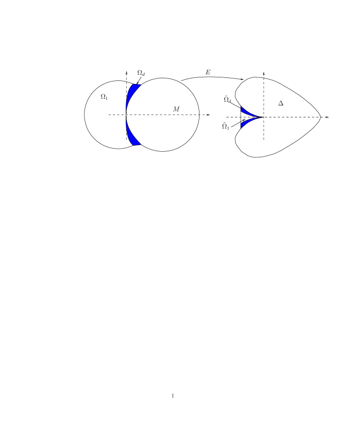
Figure 4. The existence of an extension

Let $r=(2^{-2j_{0}}+c_{1}2^{-3j_{0}})^{1/4}.$ Denote

$$M=\{(x+1,y)\in\mathbb{R}^{2}:(x,y)\in\mathbb{D}\},$$

$$\Omega_{1}=\overline{B(0,r)}\setminus(M\cup\Omega_{d}),\ \Omega_{2}=\mathbb{R}^{2}\setminus(\Omega_{1}\cup\Omega_{d}\cup M),$$

$$\tilde{\Omega}_{1}=\{(x,y)\in\mathbb{R}^{2}:x\in[-2^{-j_{0}},0],y^{2}\leq c_{1}|x|^{3}\}\mbox{ and }\tilde{\Omega}_{2}=\mathbb{R}^{2}\setminus(\tilde{\Omega}_{1}\cup\tilde{\Omega}_{d}\cup\Delta).$$

Analogously to the arguments in Section 4.1, we define $E_{1}:\Omega_{1}\rightarrow\tilde{\Omega}_{1}$ and $E_{2}:\Omega_{2}\rightarrow\tilde{\Omega}_{2}.$ Here $\eta(x)=\sqrt{x}(1+c_{1}x)^{1/4}$ and $s=3/2.$ Define

(5.0.1) $$E(x,y)=\begin{cases}E_{1}(x,y)&\forall\ (x,y)\in\Omega_{1},\\ E_{2}(x,y)&\forall\ (x,y)\in\Omega_{2},\\ (x^{2}-y^{2},2xy)&\forall\ (x,y)\in M\cup\Omega_{d},\end{cases}$$

and $f_{0}(x,y)=E(x+1,y).$ By the analogous arguments as in Section 4.1, we have that $f_{0}\in\mathcal{F}.$

We next prove (1.0.3). Suppose $f\in\mathcal{F}.$ Then $\hat{f}(u,v)=f(u-1,v)$ is a homeomorphism of finite distortion on $\mathbb{R}^{2}$ and $\hat{f}(M\setminus\Omega_{u})=\Delta\setminus\tilde{\Omega}_{u}.$ By Remark 3.1, we have that if $K_{\hat{f}}\in L^{q}_{\text{loc}}(\mathbb{R}^{2})$ then $q<2.$ Therefore if $K_{f}\in L^{q}_{\text{loc}}(\mathbb{R}^{2})$ then $q<2.$ In order to prove (1.0.3), it then suffices to construct a mapping $f_{0}\in\mathcal{F}$ such that $K_{f_{0}}\in L^{q}_{\text{loc}}(\mathbb{R}^{2})$ for all $q<2.$ Let $E$ be as in (5.0.1) and $f_{0}(x,y)=E(x+1,y).$ Then $f_{0}\in\mathcal{F}.$ The same arguments as for the case $s\in(1,2)$ in Section 4.3 show that $K_{E}\in L^{q}_{\text{loc}}(\mathbb{R}^{2})$ for all $q<2.$ Therefore $K_{f_{0}}\in L^{q}_{\text{loc}}(\mathbb{R}^{2})$ for all $q<2.$

The strategies to prove (1.0.2), (1.1), (1.0.5) and (1.0.6) are same as the one to prove (1.0.3). We leave the details to the interested reader. ∎

Haiqing Xu

Department of Mathematics and Statistics, University of Jyväskylä, PO BOX 35, FI-40014 Jyväskylä, Finland

School of Mathematical Sciences, University of Science and Technology of China, Hefei 230026, P. R. China

E-mail address: hqxu@mail.ustc.edu.cn

References

- [1] K. Astala, and M. González : Chord-arc curves and the Beurling transform. Invent. Math. 205 (2016), no. 1, 57-81.
- [2] K. Astala, T. Iwaniec, and G. J. Martin: Elliptic partial differential equations and quasiconformal mappings in the plane. Princeton Mathematical Series, 48. Princeton University Press, Princeton, NJ, 2009. xviii+677 pp.
- [3] C.-Y. Guo, P. Koskela, and J. Takkinen: Generalized quasidisks and conformality. Publ. Mat. 58 (2014), no. 1, 193-212.
- [4] C.-Y. Guo: Generalized quasidisks and conformality II. Proc. Amer. Math. Soc. 143 (2015), no. 8, 3505-3517.
- [5] S. Hencl, and P. Koskela: Regularity of the inverse of a planar Sobolev homeomorphism. Arch. Ration. Mech. Anal. 180 (2006), no. 1, 75-95.
- [6] S. Hencl, and P. Koskela: Lectures on mappings of finite distortion. Lecture Notes in Mathematics, 2096. Springer, Cham, 2014. xii+176 pp.
- [7] D. Jerison, and C. Kenig: Hardy spaces, , and singular integrals on chord-arc domains. Math. Scand. 50 (1982), no. 2, 221-247.
- [8] P. Koskela, and J. Takkinen: Mappings of finite distortion: formation of cusps. Publ. Mat. 51 (2007), no. 1, 223-242.
- [9] P. Koskela, and J. Takkinen: Mappings of finite distortion: formation of cusps. III. Acta Math. Sin. 26 (2010), no. 5, 817-824.
- [10] E. Moise: Geometric topology in dimensions and . Graduate Texts in Mathematics, Vol. 47. Springer-Verlag, New York-Heidelberg, 1977. x+262 pp
- [11] Ch. Pommerenke: Boundary behaviour of conformal maps. Grundlehren der Mathematischen Wissenschaften [Fundamental Principles of Mathematical Sciences], 299. Springer-Verlag, Berlin, 1992. x+300 pp.
- [12] S. Semmes: Quasiconformal mappings and chord-arc curves. Trans. Amer. Math. Soc. 306 (1988), no. 1, 233-263.
- [13] P. Tukia: The planar Schönflies theorem for Lipschitz maps. Ann. Acad. Sci. Fenn. Ser. A I Math. 5 (1980), no. 1, 49-72.
- [14] W. Ziemer: Weakly differentiable functions. Sobolev spaces and functions of bounded variation. Graduate Texts in Mathematics, 120. Springer-Verlag, New York, 1989. xvi+308 pp.