Reachable Space Characterization of Markov Decision Processes with Time Variability

Abstract

We propose a solution to a time-varying variant of Markov Decision Processes which can be used to address decision-theoretic planning problems for autonomous systems operating in unstructured outdoor environments. We explore the time variability property of the planning stochasticity and investigate the state reachability, based on which we then develop an efficient iterative method that offers a good trade-off between solution optimality and time complexity. The reachability space is constructed by analyzing the means and variances of states’ reaching time in the future. We validate our algorithm through extensive simulations using ocean data, and the results show that our method achieves a great performance in terms of both solution quality and computing time.

I INTRODUCTION

Autonomous vehicles that operate in the air and water are easily disturbed by stochastic environmental forces such as turbulence and currents. The motion planning in such uncertain environments can be modeled using a decision-theoretic planning framework where the substrate is the Markov Decision Processes (MDPs) [sutton2018reinforcement] and its partially observable variants [jaakkola1995reinforcement].

To cope with various sources of uncertainty, the prevalent methodology for addressing the decision-making of autonomous systems typically takes advantage of the known characterization such as probability distributions for vehicle motion uncertainties. However, the characterization of the uncertainty can vary in time with some extrinsic factors related to environments such as the time-varying disturbances in oceans as shown in Fig. 1. Despite many successful achievements [van2012motion, luo2016importance, he2010puma, martinez2007active, huang2018learning], existing work typically does not synthetically integrate environmental variability with respect to time into the decision-theoretic planning model.

Although it can be easily recognized that the time-varying stochastic properties represent a more general description of the uncertainty [QMSM2018], addressing the related planning problems is not an incremental extension to the basic time-invariant counterpart methods. This is because many components in the basic time-invariant model become time-varying terms simultaneously, requiring substantial re-modeling work and a completely new solution design. Therefore, in this work we explore the time variability of the planning stochasticity and investigate the state reachability, and these important properties allow us to gain insights for devising an efficient approach with a good trade-off between the solution optimality and the time complexity. The reachability space is constructed essentially by analyzing the first and second moments of expected future states’ reaching time. Finally, we validate our method in the scenario of navigating a marine vehicle in the ocean, and our simulation results show that the proposed approach produces results close to the optimal solution but requires much smaller computational time comparing to other baseline methods.

Figure 1: A motivating scenario: the ocean environment is highly dynamic. Autonomous vehicle planning needs to consider the strong time-varying disturbances caused by ocean currents. (Source: NASA Scientific Visualization Studio.)

II RELATED WORK

Most existing methods that solve MDPs in the literature assume time-invariant transition models [sutton2018reinforcement]. Such an assumption has also been used in most literature on reinforcement learning (RL) [Sutton1998, DayanRL08, Bagnell_2013_7451], where an agent tries to maximize accumulated rewards by interacting with its environment. A technique related to temporal analysis is temporal difference (TD) learning [Sutton88learningto, Tesauro1995TDL]. RL extends the TD technique by constantly correcting previous predictions based on the availability of new observations [Sutton1998, Boyan99least-squarestemporal]. Unfortunately, existing TD techniques are typically built on time-invariant models. Research on time variability has also been conducted in multi-agent co-learning scenarios where multiple agents learn in the environment simultaneously and enable the transition of the environment to evolve over time [he2016opponent, zheng2018deep, everett2018learning]. To tackle the environmental uncertainty, multiple stationary MDPs have been utilized to obtain better environmental representations [banerjee2017quickest, hadoux2014sequential, da2006dealing]. Policies are learned for each MDP and then switched if a context change is detected. In general, these approaches use a piece-wise stationary approximation, i.e., a time-invariant MDP is applied in each time period of a multi-period horizon.

Instead of directly modeling time-varying transition functions, exogenous variables outside of MPDs may be leveraged to characterize the variation of transition functions  [li2018faster]. Some relevant work employs partially observable MDPs to deal with non-stationary environments [choi2000environment, doshi2015bayesian], or uses Semi-Markov Decision Processes (SMDPs) to incorporate continuous action duration time in the model [Sutton99betweenmdps, puterman2014markov, jianyong2004average, beutler1986time]. However, these frameworks still essentially assume time-invariant transition models.

Recently, the time-dependent MDP has been analyzed where the space-time states are directly employed [boyan2001exact]. It has been shown that even under strong assumptions and restrictions, the computation is still prohibitive [RachelsonFG09]. Relevant but different from this model, the time-varying MDP is formulated by directly incorporating time-varying transitions whose distribution can be approximated or learned from environments [liu2018solution]. This method is compared with our proposed algorithm in the experiment section.

Reachability analysis has been vastly researched in the control community where the majority of work falls in non-stochastic domains. For example, an important framework utilizes Hamilton-Jacobi reachability analysis to guarantee control policies to drive the dynamical systems within some pre-defined safe set of states under bounded disturbances [mitchell2005time, bansal2017hamilton]. Control policies can also be learned through machine learning approaches to keep the system outside of unsafe states [gillula2012guaranteed, gillula2013reducing]. In addition, convex optimization procedures are carried out to compute reachable funnels within which the states must remain under some control policy [majumdar2017funnel]. These funnels are then used to compute robot motions online with a safety guarantee.

III Problem Formulation

We are motivated by problems that autonomous vehicles (or manipulators) move toward defined goal states under exogenous time-varying disturbances. These problems can be modeled as a time-varying Markov Decision Process.

III-A Time-Varying Markov Decision Process

We represent a time-varying Markov Decision Process (TVMDP) as a 5-tuple $(\mathbb{S},\mathbb{T},\mathbb{A},\mathcal{T},R)$. The spatial state space $\mathbb{S}$ and the action space $\mathbb{A}$ are finite. We also need an extra discrete temporal space $\mathbb{T}$ in our discussions, though our framework supports continuous time models. Because the MDP now is time-varying, an action must depend on both state and time; that is, for each state $s\in\mathbb{S}$ and each time $t\in\mathbb{T}$, we have a feasible action set $A(s,t)\subset\mathbb{A}$. The entire set of feasible state-time-action triples is $\mathbb{F}:=\{(s,t,a)\in\mathbb{S}\times\mathbb{T}\times\mathbb{A}\}$. There is a probability transition law $\mathcal{T}(s,t,a;\cdot,\cdot)$ on $\mathbb{S}\times\mathbb{T}$ for all $(s,t,a)\in\mathbb{F}$. Thus, $\mathcal{T}(s,t,a;s^{\prime},t^{\prime})$ specifies the probability of transitioning to state $s^{\prime}$ at a future time $t^{\prime}$ given the current state $s$ and time $t$ ($t\leq t^{\prime}$) under action $a$. The final element $R:\mathbb{F}\rightarrow\mathbb{R}^{1}$ is a real-valued reward function that depends on the state-time-action triple.

Comparing with the classic MDP representation, TVMDP contains an additional time space $\mathbb{T}$; the transition law $\mathcal{T}$ and the reward function depend on the state, action, and time. Therefore, the major difference between TVMDPs and classic MDPs is that the transition probability and reward function are time-dependent.

We consider the class of deterministic Markov policies [puterman2014markov], denoted by $\Pi$; that is, the mapping $\pi\in\Pi:\mathbb{S}\times\mathbb{T}\rightarrow\mathbb{A}$ depends on the current state and the current time, and $\pi(s,t)\in A(s,t)$ for a given state-time pair. The initial state $s_{0}\in\mathbb{S}$ at time $t=0$ and policy $\pi\in\Pi$ determine a stochastic trajectory (path) process $\tau:=\{(s_{t},a_{t})\}_{t\geq 0}$. The two terms, path and trajectory, will be used interchangeably. For a given initial state $s_{0}$ and starting time $t_{0}$, the expected discounted total reward is represented as:

$$v^{\pi}(s_{0},t_{0})=\mathbb{E}^{\pi}_{s_{0},t_{0}}\left[\sum_{k=0}^{\infty}\gamma^{k}R(s_{k},t_{k},a_{k})\right],$$ (1)

where $\gamma\in[0,1)$ is the discount factor that discounts the reward at a geometric decaying rate. Our aim is to find a policy $\pi^{*}$ to maximize the total reward from the starting time $t_{0}$ at the initial state $s_{0}$, i.e.,

$$\pi^{*}(s_{0},t_{0})=\operatorname*{arg\,max}_{\pi\in\Pi}v^{\pi}(s_{0},t_{0}).$$ (2)

Accordingly, the optimal value is denoted by $v^{*}(s_{0},t_{0})$.

III-B Passage Percolation Time

The 2D plane in which the autonomous system operates is modeled as the spatial state space. The plane is discretized into grids, and the center of each grid represents a state. Two spatial states are connected if their corresponding grids are neighbors, i.e. a vehicle in one grid is able to transit to the other grid directly without passing through any other grids. Because the vehicle motion follows physical laws (e.g., motion kinematics and dynamics), travel time is required for the vehicle to transit between two different states. Let $h(s,t,s^{\prime})$ be the local transition time for a vehicle to travel from state $s$ at time $t$ to a connected state $s^{\prime}$. Such a local transition time is time-dependent and is assumed deterministic.

If, however, the two states $s$ and $s^{\prime}$ are not connected, then the transition time between them is a random variable and depends on the trajectory of the vehicle. For any finite path $\tau=\{(s,a_{0}),...,(s^{\prime},a_{n})\}_{n>0}$ starting from time $u$ at state $s$ and ending with state $s^{\prime}$, we define the Passage Percolation Time (PPT) between $s$ and $s^{\prime}$ to be

$$H_{s,s^{\prime}}^{u}=\sum_{(s_{k},a_{k})\in\tau}h(s_{k},t_{k},s_{k+1}),$$ (3)

where $t_{0}=u,t_{k}=t_{k-1}+h(s_{k-1},t_{k-1},s_{k})$ and $0<k<n$. In addition, we require $H_{s,s}^{u}=0$. By definition it is the transition time (travel time) on a path from the state $s$ at time $u$ until firstly reaching the state $s^{\prime}$ [auffinger201550, grimmett1999percolation]. If the local transition time $h$ does not depend on time, the definition of Eq.(3) is exactly the same as the conventional passage time for percolation [auffinger201550]. We would like to emphasize that $H^{u}_{s,s^{\prime}}$ is a random variable, which relies on the realized path between $s$ and $s^{\prime}$. Under the policy $\pi$, the mean and variance of the PPT are assumed to exist, and are denoted by $\mu^{\pi}_{s,u;s^{\prime}}:=\mathbb{E}^{\pi}[H^{u}_{s,s^{\prime}}]$ and $(\sigma^{\pi}_{s,u;s^{\prime}})^{2}=\mathbb{V}^{\pi}[H^{u}_{s,s^{\prime}}]$, respectively.

III-C Spatiotemporal State Space Representation

One can view a TVMDP as a classic MDP by defining the product of both spatial and temporal spaces $\mathbb{S}\times\mathbb{T}$ as a new state space $\mathbb{S}^{\prime}$. Namely, the state space now stands for the spatiotemporal space in our context. In this representation, one can imagine that the spatial state space $\mathbb{S}$ is duplicated on every discrete time “layer" to form a collection of spatial states along the temporal dimension as $\{\mathbb{S}_{1},\mathbb{S}_{2},...\}$, where each $\mathbb{S}_{k}$ is the same as $\mathbb{S}$. The state-time pair $(s,t)$ corresponds to a state in this spatiotemporal space. Transition links are added by concatenating states on different time layers, constrained by the local transition time $h$. Similar spatiotemporal representation is also adopted in many other fields [shang2019integrating, boyan2001exact, MAHMOUDI201619].

We emphasize here that the discrete time intervals and transition links between states in the spatiotemporal representation can be determined by the underlying motion kinematics of autonomous vehicles via the local transition time. This is a time discretization-free mechanism and is naturally supported by our proposed TVMDP framework. We will show an example in Section LABEL:sec:realistic.

III-D TVMDP Value Iteration in Spatiotemporal Space

The optimal policy $\pi^{*}$ for TVMDPs may be conceptually achieved by the conventional value iteration approach through sweeping the entire state space $\mathbb{S}$ and time space $\mathbb{T}$. The TVMDP value iteration (VI) amounts to iterating the following state-time value function until convergence,

$$v(s,t)=\max_{a\in A(s,t)}\left\{R(s,t,a)+\gamma\cdot\mathbb{E}[v(s^{\prime},t^{\prime})\mid s,a;t]\right\},$$ (4)

where $s^{\prime}$ is the next state to visit at time $t^{\prime}$ from the current state $s$ at time $t$, and

$$\mathbb{E}[v(s^{\prime},t^{\prime})\mid s,a;t]=\sum_{s^{\prime}\in\mathbb{S},t^{\prime}\in\mathbb{T}}\mathcal{T}(s,t,a;s^{\prime},t^{\prime})\cdot v(s^{\prime},t^{\prime})$$

is the weighted average of the value functions of all the next possible spatiotemporal states.

The value function Eq. (4) is a modification of the conventional Bellman equation as it includes a notion of time. In addition to propagating values spatially from next states, it also backs up the value temporally from a future time. Moreover, the benefits of the spatiotemporal representation in applications are readily seen, as the solution to Eq. (4) is equivalent to applying dynamic programming directly to the spatiotemporal state space.

A typical spatiotemporal state space is very large, especially when high state resolution is needed. The naive dynamic programming-based value iteration or policy iteration involves backing up state-values not only from the spatial dimension but also from the temporal dimension. It is generally intractable to solve for the exact optimal policy due to the so-called curse of dimensionality [liu2016mdp].

IV Methodology

In this section, we present tractable iterative algorithms for TVMDP by a reduction of the spatiotemporal state space in each iteration. Our approach is grounded in characterizing the most possibly reachable set of states through the first and second moments of the passage percolation time.

IV-A Overview

One of the major challenges to solving the Bellman equation (Eq. (4)) is the search in a large spatiotemporal state space. Once we are able to reduce the whole spatiotemporal space to a tractable size, it is then possible to obtain solutions by, for instance, the value iteration algorithm, within a reasonable time span. Given a policy, an initial state-time pair, and a probability transition law, for a fixed (spatial) state $s$, probabilities of visiting $s$ at different times are highly likely different. If we are able to quantify the reachability of spatiotemporal states by visiting probability, and trim the whole spatiotemporal space by removing those with small reachability, it is highly likely that the optimal total reward will not be affected much (under certain restrictions on the variability of the reward and transition functions), and we can gain significant benefits from reducing the computation.

The previously introduced variable Passage Percolation Time (PPT) $H^{u}_{s,s^{\prime}}$ sheds light on estimating the chances of reaching state $s^{\prime}$ by evaluating the transition time from a state $s$ at time $u$. Although the exact probability distribution of PPT is generally hard to obtain, its first and second moments are relatively easy to compute. Therefore, we use the expectation and variance of PPT between the initial spatial state $s_{0}$ and another arbitrary state $s$ to characterize the most possible time interval to reaching $s$. Following this way, we are able to find a most reachable set $\{(s,t)\}_{t\in\mathbb{T}}$ along the spatiotemporal dimensions. This reachable set is closed, allowing us to reduce the search by looking only within the enclosed spatiotemporal space.

The above procedure actually views all $H^{u}_{s_{0},s}$ independently, and does not compute the probability for every trajectory. If one state-action pair in a trajectory is removed, the associated trajectory will become invalid in the reduced space. Therefore, it may eliminate too many potential trajectories (paths) $\tau$ with relatively large probability. In order to remedy this problem, we reconstruct a TVMDP on the reduced spatiotemporal space to maintain a certain correlation between connected spatial states (recall the definition of connection in section III-B). In Section LABEL:sec:final-algorithm, we will see this procedure is equivalent to mapping a removed potential trajectory to another one in the reduced search space.

The final algorithm iterates the above procedures on the whole spatiotemporal space. In each iterative step, the first and second moments of the PPT are recomputed. Intuitively, the first moment is used to find the “backbone" that outlines the most reachable states, whereas the second moment determines the “thickness" (or volume) of the most reachable space. The policy is then updated on the reduced space, and the actions for states outside the reduced space are mapped to the updated actions on nearest states in the reduced space. Comparing with [liu2018solution] which only uses the first moment of PPT to characterize TVMDP, our method obtains a better approximation to the full spatiotemporal space of TVMDP.

IV-B Value Iteration with Expected Passage Percolation Time

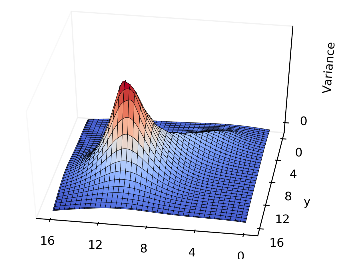
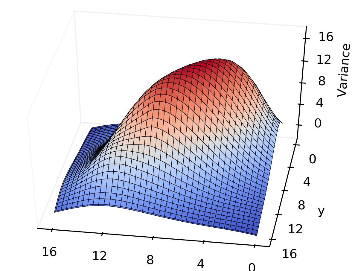
Figure 2: The change in the variance under different uncertainties in the environment. The state transition is modeled as a Gaussian distribution which is referred to Sec. LABEL:sec:experiment. (a)(b) 3D and top down views with the variance of the transition function set to $0.1$. (c)(d) A more uncertain environment with the variance set to $1$.

This section presents the first approximate algorithm, an expected PPT-based value iteration, for TVMDPs. It serves as a burn-in procedure for the algorithm in Section LABEL:sec:final-algorithm.

In this first approximate algorithm, we use the transition probabilities and the reward function at the expected PPTs to approximate their time-varying counterpart. Then we approximate the TVMDP by an MDP with a properly defined action set at $s$. Accordingly, we can conduct value iteration on the state space $\mathbb{S}$ rather than space $\mathbb{S}\times\mathbb{T}$, and use the resulting time-independent policy for the state at any time.

Suppose $\mu_{s}:=\mathbb{E}^{\pi}[H^{t_{0}}_{s_{0},s}]$ are already obtained for all $s\in\mathbb{S}$ given the initial state $s_{0}$ and the starting time $t_{0}$. Note that we always have $\mu_{s_{0}}=0$. With a new transition probability law defined as $\mathcal{T}^{\pi,\mu_{s}}_{s,s^{\prime}}:=\sum_{t^{\prime}}\mathcal{T}(s,\mu_{s},a;s^{\prime},t^{\prime})$ and a new reward function as $R^{\mu_{s}}(s,a):=R(s,a,\mu_{s})$, one can update the policy by solving the following Bellman equation

$$v(s)=\max_{a\in A(s)}\left\{R^{\mu_{s}}(s,a)+\gamma\cdot\mathbb{E}^{\pi}_{\mu_{s}}[v(s^{\prime})\mid s,a]\right\},$$ (5)

where $\mathbb{E}^{\pi}_{\mu_{s}}(\cdot)$ indicates the calculation under the new transition law $\mathcal{T}^{\pi,\mu_{s}}_{s,s^{\prime}}$ and $A(s)$ is the action set at $s$. The output policy does not depend on time anymore, and will be used for any state all the time. Usually we only have one $t^{\prime}\in\mathbb{T}$ such that $\mathcal{T}(s,u,a;s^{\prime},t^{\prime})>0$ for fixed $s,u,a$ and $s^{\prime}$ in the practical modeling framework. If $t^{\prime\prime}\neq t^{\prime}$, then $\mathcal{T}(s,u,a;s^{\prime},t^{\prime\prime})=0$. In this case, $\mathcal{T}^{\pi,\mu_{s}}_{s,s^{\prime}}=\mathcal{T}(s,\mu_{s},a;s^{\prime},t^{\prime})$. Now we show how to obtain the expected PPTs. By the conditional expectation formula $\mathbb{E}^{\pi}[H_{s,s^{\prime}}^{u}]=\mathbb{E}^{\pi}[H_{s^{\prime\prime},s^{\prime}}^{u}\mid s^{\prime\prime}]$, the expected PPTs satisfy the following linear system

$$\mathbb{E}^{\pi}[H_{s,s^{\prime}}^{u}] =\sum_{s^{\prime\prime},u^{\prime\prime}}\mathcal{T}(s,a,u;s^{\prime},u^{\prime\prime})\left(h(s,u,s^{\prime\prime})+\mathbb{E}^{\pi}[H_{s^{\prime\prime},s^{\prime}}^{u^{\prime\prime}}]\right)$$ (6a)

$$\mathbb{E}^{\pi}[H_{s,s}^{u}] =0,$$ (6b)

where $s\neq s^{\prime}$, $u^{\prime\prime}=u+h(s,u,s^{\prime\prime})$, and $s^{\prime\prime}$ in Eq. (6a) is the next visiting state from $s$. The above recursive relationship is similar to the equations for estimating the mean first passage time for a Markov Chain [Jeffrey2018, debnath2018solving], except that the mean first passage time from a state to itself is a positive value.

We do not solve Eq. (6) for all time $u$ altogether. Instead, we approximate the solutions in a recursive fashion with the aim of estimating $\mu_{s}$ for all $s$ in the space. In other words, we only carry the estimates of $\mu_{s}$ into the next iteration. In each iteration, we approximate Eq. (6a) by the following linear system

$$\mathbb{E}^{\pi}[H_{s,s^{\prime}}^{\tilde{\mu}_{s}}] =\sum_{s^{\prime\prime}}\mathcal{T}^{\pi,\tilde{\mu}_{s}}_{s,s^{\prime\prime}}\left(h(s,\tilde{\mu}_{s},s^{\prime\prime})+\mathbb{E}^{\pi}[H_{s^{\prime\prime},s^{\prime}}^{\tilde{\mu}_{s^{\prime\prime}}}]\right),$$ (7)

where $\tilde{\mu}_{s}=\mathbb{E}^{\tilde{\pi}}(H^{t_{0}}_{s_{0},s})$ are obtained from the latest iteration with the previous policy $\tilde{\pi}$. It should be noted that one only needs to solve a linear system which consists of $(N-1)$ linear equations with $N-1$ unknown variables for one $\mu_{s}$. Here, $N:=|\mathbb{S}|$ denote the total number of states. Therefore, we merely need to solve $(N-1)$ linear systems to obtain all $\mu_{s}$ in one iteration step.