Kernel Wasserstein Distance

Abstract

The Wasserstein distance is a powerful metric based on the theory of optimal transport. It gives a natural measure of the distance between two distributions with a wide range of applications. In contrast to a number of the common divergences on distributions such as Kullback-Leibler or Jensen-Shannon, it is (weakly) continuous, and thus ideal for analyzing corrupted data. To date, however, no kernel methods for dealing with nonlinear data have been proposed via the Wasserstein distance. In this work, we develop a novel method to compute the L²-Wasserstein distance in a kernel space implemented using the kernel trick. The latter is a general method in machine learning employed to handle data in a nonlinear manner. We evaluate the proposed approach in identifying computerized tomography (CT) slices with dental artifacts in head and neck cancer, performing unsupervised hierarchical clustering on the resulting Wasserstein distance matrix that is computed on imaging texture features extracted from each CT slice. Our experiments show that the kernel approach outperforms classical non-kernel approaches in identifying CT slices with artifacts.

1 Introduction

Optimal mass transport (OMT) theory is an old research area with its roots in civil engineering (Monge 1781) and economics (Kantorovich 1942) [1]. Recently there has been an ever increasing growth in OMT research both theoretically and practically, with impact on numerous fields including medical imaging analysis, statistical physics, machine learning, and genomics [2, 3, 4, 5]. The classical OMT problem formulated by Monge in 1781 concerns finding the optimal way via the minimization of a transportation cost required to move a pile of soil from one site to another [6, 7, 8, 9]. Let $X$ and $Y$ denote two probability spaces with measures $\mu$ and $\nu$, respectively, and let $c(x,y)$ denote the transportation cost for moving one unit of mass from $x\in X$ to $y\in Y$. Then the OMT problem seeks to find a (measurable) transport map $T:X\rightarrow Y$ that minimizes the total transportation cost $\int_{X}c(x,T(x)){\rm\mu}(dx)$. In 1942, Kantorovich proposed a relaxed formulation that transforms the Monge’s nonlinear problem to a linear programming problem [8]. Based on the Kantorovich’s formulation, the ${\it L^{p}}$- Wasserstein distance between $\mu$ and $\nu$ on $\mathcal{R}^{d}$ is defined as:

$$W_{p}^{p}\left({\bf\mu},{\bf\nu}\right)={\rm\inf}_{\pi\in\Pi(\mu,\nu)}\int_{{\rm R}^{d}\times{\rm R}^{d}}{\|{x}-{y}\|}^{p}d\pi(x,y),$$ (1)

where $\Pi(\mu,\nu)$ is the set of all joint probability measures $\pi$ on $X\times Y$ whose marginals are $\mu$ and $\nu$. In particular, in this study, we focus on $\it L^{\rm 2}$- Wasserstein distance in which the squared Euclidean distance $c(x,y)={\|{x}-{y}\|}^{2}$ is the cost function [10]. Before introducing our proposed kernel Wasserstein distance, we first review some background on the kernel method.

The kernel space method is based on the following idea. Suppose that we are given a data set of $n$ samples in a native space, denoted by ${\bf X}=[{\bf x}_{1},{\bf x}_{2},\cdots,{\bf x}_{\it n}]\in\mathcal{R}^{d}$. The input data can be mapped (transformed) into a higher dimensional feature space (called the kernel space) via a nonlinear mapping function $\phi$ [11, 12]. Let ${\bf\Phi}$ be ${\bf\Phi}_{l\times n}=[\phi({\bf x}_{1}),\phi({\bf x}_{2}),\cdots,\phi(\bf x_{\it n})]$, i.e., the transformed data, where $l$ is the number of features in the feature (kernel) space with $l>d$. To avoid complex data handling in the feature space, and to avoid the explicit computation of the mapping funciton $\phi$, typically one applies the kernel trick. More precisely, given any positive definite kernel function $k$, one can find an associated mapping function $\phi$ such that $k({\bf x},{\bf y})=<\phi{({\bf x})},\phi{({\bf y})}>$ with ${\bf x},{\bf y}\in\mathcal{R}^{d}$ [13, 14]. The resulting kernel Gram matrix ${\bf K}$ is defined as:

$${\bf K}={\bf\Phi}^{\rm T}{\bf\Phi},$$ (2)

where the $ij$th element, $\phi({\bf x}_{i})^{\rm T}\phi({\bf x}_{j})$, is computed using a kernel function $k({{\bf x}_{i},{\bf x}_{j}})=<\phi{({\bf x}_{i})},\phi{({\bf x}_{j})}>$. Common choices of kernel functions are the polynomial and radial basis function (RBF) kernels. In this study, the following RBF kernel will be employed:

$$k({{\bf x}_{i},{\bf x}_{j}})={\rm exp}\big{(}-\gamma||{{\bf x}_{i}-{\bf x}_{j}}||^{2}\big{)},$$ (3)

where $\gamma>0$ controls the kernel width. We will fix $\gamma=1$ in what follows. The mean and the covariance matrix in the feature space are estimated as:

$${\bf\mu}=\frac{1}{n}\sum_{i=1}^{n}\phi({\bf x}_{\it i})={\bf\Phi s},{~{}~{}~{}\rm and~{}~{}~{}}{\bf\Sigma}=\frac{1}{n}\sum_{i=1}^{n}(\phi({\bf x}_{\it i})-{\bf\mu})(\phi({\bf x}_{\it i})-{\bf\mu})^{\rm T}={\bf\Phi JJ^{\rm T}\Phi^{\rm T}},$$ (4)

where ${\bf s}_{n\times 1}=\frac{1}{n}{\bf\vec{1}}^{\rm T}$, $\bf{J}=\frac{\rm 1}{\sqrt{\it{n}}}(\bf I_{\it n}-s{\bf\vec{1}})$, and ${\bf\vec{1}}=[1,1,\cdots,1]$. Then in Eq. (4), denoting $\bf{\Phi J}$ by ${\bf W}$ we have

$$\bf{W=\Phi J}=\frac{\rm 1}{\sqrt{\it{n}}}[(\phi({\bf x}_{\rm 1})-{\bf\mu}),\cdots,(\phi({\bf x}_{\it n})-{\bf\mu})].$$ (5)

Of note, these equations are used to compute the kernel Wasserstein distance as described in the following section.

2 Methods

In this section, we introduce the classical L²-Wasserstein distance between Gaussian measures and then propose a novel approach to compute L²-Wasserstein distance in the kernel space (denoted as kernel L²-Wasserstein distance). For comparison, we also provide a brief review of the Kullback-Leibler distance in the kernel space that we proposed in [15]. The code was implemented using MATLAB R2018b.

2.1 L²-Wasserstein Distance

For two Gaussian measures, $\nu_{1}=N_{1}({\bf m}_{\rm 1},{\bf C}_{\rm 1})$ and $\nu_{2}=N_{2}({\bf m}_{\rm 2},{\bf C}_{\rm 2})$ on $\mathcal{R}^{d},$ the L²-Wasserstein distance between the two distributions may be computed as follows [16]:

$$W_{2}(\nu_{1},\nu_{2})^{2}=\|{\bf m}_{\rm 1}-{\bf m}_{\rm 2}\|^{2}+{\rm tr}({\bf C}_{\rm 1}+{\bf C}_{\rm 2}-2({\bf C}_{\rm 1}^{\frac{1}{2}}{\bf C}_{\rm 2}{\bf C}_{\rm 1}^{\frac{1}{2}})^{\frac{1}{2}}),$$ (6)

where ${\rm tr}$ is the trace. The term ${\rm tr}({\bf C}_{\rm 1}+{\bf C}_{\rm 2}-2({\bf C}_{\rm 1}^{\frac{1}{2}}{\bf C}_{\rm 2}{\bf C}_{\rm 1}^{\frac{1}{2}})^{\frac{1}{2}})$ can be expressed as follows [17, 18, 19]:

$${\rm tr}({\bf C}_{1}+{\bf C}_{2}-2({\bf C}_{2}{\bf C}_{1})^{\frac{1}{2}}).$$ (7)

For convenience, we sketch the proof of this fact.

Proof.

By the property of trace, ${\rm tr}({\bf C}_{1}+{\bf C}_{2}-2({\bf C}_{2}{\bf C}_{1})^{\frac{1}{2}})={\rm tr}({\bf C}_{1})+{\rm tr}({\bf C}_{2})-2{\rm tr}({\bf C}_{2}{\bf C}_{1})^{\frac{1}{2}}.$ Therefore, we need to prove that ${\rm tr}({\bf C}_{2}{\bf C}_{1})^{\frac{1}{2}}={\rm tr}({\bf C}_{\rm 1}^{\frac{1}{2}}{\bf C}_{\rm 2}{\bf C}_{\rm 1}^{\frac{1}{2}})^{\frac{1}{2}}$. Note that ${\bf C}_{\rm 1}$ and ${\bf C}_{\rm 2}$ are symmetric positive semidefinite, and ${\bf C}_{\rm 2}{\bf C}_{\rm 1}$ is diagonalizable and has nonnegative eigenvalues [20]. The eigenvalue decomposition of ${\bf C}_{2}{\bf C}_{1}$ can be computed as ${\bf C}_{2}{\bf C}_{1}{\bf P}={\bf P\Lambda}$ where ${\bf P}$ and $\Lambda$ are the estimated eigenvector and eigenvalue matrices, respectively. Multiplying both sides by ${\bf C}_{1}^{\frac{1}{2}}$, we have ${\bf C}_{1}^{\frac{1}{2}}{\bf C}_{2}{\bf C}_{1}^{\frac{1}{2}}{\bf C}_{1}^{\frac{1}{2}}{\bf P}={\bf C}_{1}^{\frac{1}{2}}{\bf P\Lambda}.$ That is, ${\bf C}_{1}^{\frac{1}{2}}{\bf C}_{2}{\bf C}_{1}^{\frac{1}{2}}$ has an eigenvector matrix ${\bf C}_{1}^{\frac{1}{2}}{\bf P}$ and an eigenvalue matrix ${\bf\Lambda}$ which is the same as that of ${\bf C}_{2}{\bf C}_{1}$ [21]. Let $\lambda_{1},\lambda_{2},...,\lambda_{k}$ be the distinct eigenvalues of ${\bf C}_{2}{\bf C}_{1}$. Then the eigenvalues of $({\bf C}_{2}{\bf C}_{1})^{\frac{1}{2}}$ are $\sqrt{\lambda_{1}},\sqrt{\lambda_{2}},...,\sqrt{\lambda_{k}}$. Therefore, ${\rm tr}({\bf C}_{2}{\bf C}_{1})^{\frac{1}{2}}={\rm tr}({\bf C}_{\rm 1}^{\frac{1}{2}}{\bf C}_{\rm 2}{\bf C}_{\rm 1}^{\frac{1}{2}})^{\frac{1}{2}}$. ∎

In particular, when ${\bf C}_{1}={\bf C}_{2}$, we have $W_{2}(\nu_{1},\nu_{2})^{2}=\|{\bf m}_{\rm 1}-{\bf m}_{\rm 2}\|^{2}.$

2.2 L²-Wasserstein Distance in Kernel Space

Suppose that we are given two Gaussian measures, $k\nu_{1}$ and $k\nu_{2}\in\mathcal{R}^{\it l}$, in the kernel space with mean ${\bf\mu}_{\it i}$ and covariance matrix ${\bf\Sigma}_{\it i}$, for ${\it i}$=1 and 2, and two sets of sample data in the native space, ${\bf X}=[{\bf x}_{1},{\bf x}_{2},\cdots,{\bf x}_{\it n}],\;{\bf Y}=[{\bf y}_{1},{\bf y}_{2},\cdots,{\bf y}_{\it m}]\in\mathcal{R}^{d}$ associated with $k\nu_{1}$ and $k\nu_{2}$, respectively. Then, as in Eq. (6), the L²-Wasserstein distance between the two distributions is given by:

$$W_{2}(k\nu_{1},k\nu_{2})^{2}=\|{\bf\mu}_{\rm 1}-{\bf\mu}_{\rm 2}\|^{2}+{\rm tr}({\bf\Sigma}_{\rm 1}+{\bf\Sigma}_{\rm 2}-2({\bf\Sigma}_{\rm 1}^{\frac{1}{2}}{\bf\Sigma}_{\rm 2}{\bf\Sigma}_{\rm 1}^{\frac{1}{2}})^{\frac{1}{2}}),$$ (8)

where the definitions of ${\bf\mu}_{\it i}$ and ${\bf\Sigma}_{\it i}$ are shown in Eq. (4). Note that ${\rm tr}({\bf\Sigma}_{\rm 1}^{\frac{1}{2}}{\bf\Sigma}_{\rm 2}{\bf\Sigma}_{\rm 1}^{\frac{1}{2}})^{\frac{1}{2}}={\rm tr}\left({\bf\Sigma}_{2}{\bf\Sigma}_{1}\right)^{\frac{1}{2}}$. The first term, $\|{\bf\mu}_{\rm 1}-{\bf\mu}_{\rm 2}\|^{2}$, in Eq. (8) can be obtained as follows [22]:

$$\|{\bf\mu}_{1}-{\bf\mu}_{2}\|^{2}=\|{\bf\mu}_{1}\|^{2}-2{\bf\mu}_{1}^{\rm T}{\bf\mu}_{2}+\|{\bf\mu}_{2}\|^{2}.$$ (9)

Via a simple computation, Eq. (9) can be expressed as:

$$\|{\bf\mu}_{1}-{\bf\mu}_{2}\|^{2}=\frac{1}{n^{2}}\sum_{i=1}^{n}\sum_{j=1}^{n}{\it k}\left({\bf x}_{i},{\bf x}_{j}\right)-\frac{2}{nm}\sum_{i=1}^{n}\sum_{j=1}^{m}{\it k}\left({\bf x}_{i},{\bf y}_{j}\right)+\frac{1}{m^{2}}\sum_{i=1}^{m}\sum_{j=1}^{m}{\it k}\left({\bf y}_{i},{\bf y}_{j}\right).$$ (10)

Now we simplify the last term in Eq. (8) by using Eq. (4) :
$~{}~{}~{}~{}~{}~{}~{}~{}~{}~{}~{}~{}~{}~{}~{}~{}~{}~{}~{}~{}{\rm tr}({\bf\Sigma}_{1}+{\bf\Sigma}_{2}-2({\bf\Sigma}_{2}{\bf\Sigma}_{1})^{\frac{1}{2}})={\rm tr}\left({\bf\Sigma}_{1}\right)+{\rm tr}\left({\bf\Sigma}_{2}\right)-2{\rm tr}\left({\bf\Sigma}_{2}{\bf\Sigma}_{1}\right)^{\frac{1}{2}}$

$$= {\rm tr}\left({\bf\Phi}_{1}{\bf J}_{1}{\bf J}_{1}^{\rm T}{\bf\Phi}_{1}^{\rm T}\right)+{\rm tr}\left({\bf\Phi}_{2}{\bf J}_{2}{\bf J}_{2}^{\rm T}{\bf\Phi}_{2}^{\rm T}\right)-2{\rm tr}\left({\bf\Phi}_{2}{\bf J}_{2}{\bf J}_{2}^{\rm T}{\bf\Phi}_{2}^{\rm T}{\bf\Phi}_{1}{\bf J}_{1}{\bf J}_{1}^{\rm T}{\bf\Phi}_{1}^{\rm T}\right)^{\frac{1}{2}}$$

$$= {\rm tr}\left({\bf J}_{1}{\bf J}_{1}^{\rm T}{\bf\Phi}_{1}^{\rm T}{\bf\Phi}_{1}\right)+{\rm tr}\left({\bf J}_{2}{\bf J}_{2}^{\rm T}{\bf\Phi}_{2}^{\rm T}{\bf\Phi}_{2}\right)-2{\rm tr}\left({\bf\Phi}_{2}{\bf J}_{2}{\bf J}_{2}^{\rm T}{\bf K}_{21}{\bf J}_{1}{\bf J}_{1}^{\rm T}{\bf\Phi}_{1}^{\rm T}\right)^{\frac{1}{2}}$$ (11)

$$= {\rm tr}\left({\bf J}_{1}{\bf J}_{1}^{\rm T}{\bf K}_{11}\right)+{\rm tr}\left({\bf J}_{2}{\bf J}_{2}^{\rm T}{{\bf K}_{22}}\right)-2{\rm tr}\left({\bf\Phi}_{2}{\bf R}{\bf\Phi}_{1}^{\rm T}\right)^{\frac{1}{2}},$$

where ${\bf R}={\bf J}_{2}{\bf J}_{2}^{\rm T}{\bf K}_{21}{\bf J}_{1}{\bf J}_{1}^{\rm T}$ and ${\bf K}_{\it ij}={\bf\Phi}_{i}^{\rm T}{\bf\Phi_{\it j}}$. Note that ${\bf\Sigma_{\rm 1}}$ and ${\bf\Sigma_{\rm 2}}$ are symmetric positive semidefinite. Therefore, ${\bf\Sigma_{\rm 2}}{\bf\Sigma_{\rm 1}}={\bf\Phi}_{2}{\bf R}{\bf\Phi}_{1}^{\rm T}$ is diagonalizable and has nonnegative eigenvalues. Suppose that the eigenvector and eigenvalue matrices of ${\bf\Phi}_{2}{\bf R}{\bf\Phi}_{1}^{\rm T}$ are $\bf\tilde{P}$ and ${\bf\tilde{\Lambda}}$:

$${\bf\Phi}_{2}{\bf R}{\bf\Phi}_{1}^{\rm T}{\bf\tilde{P}}={\bf\tilde{P}\tilde{\Lambda}}.$$ (12)

By multiplying both sides by ${\bf\Phi}_{1}^{\rm T}$, we have ${\bf\Phi}_{1}^{\rm T}{\bf\Phi}_{2}{\bf R}{\bf\Phi}_{1}^{\rm T}{\bf\tilde{P}}={\bf\Phi}_{1}^{\rm T}{\bf\tilde{P}\tilde{\Lambda}}$. That is, the eigenvalue matrix of ${\bf\Phi}_{1}^{\rm T}{\bf\Phi}_{2}{\bf R}$ is the same as that of ${\bf\Phi}_{2}{\bf R}{\bf\Phi}_{1}^{\rm T}$ with ${\bf\tilde{\Lambda}}$. Therefore, the following equations hold:

$${\rm tr}\left({\bf\Phi}_{2}{\bf R}{\bf\Phi}_{1}^{\rm T}\right)^{\frac{1}{2}}={\rm tr}\left({\bf\Phi}_{1}^{\rm T}{\bf\Phi}_{2}{\bf R}\right)^{\frac{1}{2}}={\rm tr}\left({\bf K}_{12}{\bf R}\right)^{\frac{1}{2}}={\rm tr}\left({\bf K}_{12}{\bf J}_{2}{\bf J}_{2}^{\rm T}{\bf K}_{21}{\bf J}_{1}{\bf J}_{1}^{\rm T}\right)^{\frac{1}{2}}.$$ (13)

Finally, using Eq. (10) and Eq. (13), the kernel L²-Wasserstein distance can be expressed as:
$W_{2}(k\nu_{1},k\nu_{2})^{2}$=$\|{\bf\mu}_{1}-{\bf\mu}_{2}\|^{2}+{\rm tr}({\bf\Sigma}_{1}+{\bf\Sigma}_{2}-2({\bf\Sigma}_{1}^{\frac{1}{2}}{\bf\Sigma}_{2}{\bf\Sigma}_{1}^{\frac{1}{2}})^{\frac{1}{2}})$

$${~{}~{}~{}~{}~{}~{}~{}~{}~{}~{}~{}~{}~{}~{}~{}~{}~{}~{}~{}~{}}=\frac{1}{n^{2}}\sum_{i=1}^{n}\sum_{j=1}^{n}{\it k}\left({\bf x}_{i},{\bf x}_{j}\right)-\frac{2}{nm}\sum_{i=1}^{n}\sum_{j=1}^{m}{\it k}\left({\bf x}_{i},{\bf y}_{j}\right)+\frac{1}{m^{2}}\sum_{i=1}^{m}\sum_{j=1}^{m}{\it k}\left({\bf y}_{i},{\bf y}_{j}\right)+$$ (14)

$${\rm tr}\left({\bf J}_{1}{\bf J}_{1}^{\rm T}{\bf K}_{11}\right)+{\rm tr}\left({\bf J}_{2}{\bf J}_{2}^{\rm T}{\bf K}_{22}\right)-2{\rm tr}\left({\bf K}_{12}{\bf J}_{2}{\bf J}_{2}^{\rm T}{\bf K}_{21}{\bf J}_{1}{\bf J}_{1}^{\rm T}\right)^{\frac{1}{2}}.$$

In a special case, when ${\bf\Sigma}_{1}={\bf\Sigma}_{2}$, we have $W_{2}(k\nu_{1},k\nu_{2})^{2}=\frac{1}{n^{2}}\sum_{i=1}^{n}\sum_{j=1}^{n}{\it k}\left({\bf x}_{i},{\bf x}_{j}\right)-\frac{2}{nm}\sum_{i=1}^{n}\sum_{j=1}^{m}{\it k}\left({\bf x}_{i},{\bf y}_{j}\right)+\frac{1}{m^{2}}\sum_{i=1}^{m}\sum_{j=1}^{m}{\it k}\left({\bf y}_{i},{\bf y}_{j}\right)$.

2.3 Kullback-Leibler Divergence in Kernel Space

Kullback-Leibler (KL) divergence is another type of method to compare two probability distributions [23]. It is not a distance measure due to its asymmetric nature. Let $P$ and $Q$ be two continuous probability distributions with the corresponding probability densities $p(x)$ and $q(x)$, respectively. Then the KL divergence or relative entropy of $P$ and $Q$ over the same variable $x$ is defined as:

$$D_{\mathrm{KL}}(P\|Q)=\int_{-\infty}^{\infty}p({x})\log\frac{p({x})}{q({x})}{dx},$$ (15)

where $D_{\mathrm{KL}}(P\|Q)$ equals zero if and only if $P=Q$. Given two Gaussian measures in the kernel space, ${N}_{1}({\bf\mu}_{1},{\bf\Sigma}_{1})$ and ${N}_{2}({\bf\mu}_{2},{\bf\Sigma}_{2})$ with both $\in\mathcal{R}^{\it l}$, the KL divergence may be computed to be:

$$D_{\rm KL}({N}_{1}||{N}_{2})=\frac{1}{2}\big{\{}({\bf\mu}_{1}-{\bf\mu}_{2})^{\bf{\rm T}}{\bf\Sigma}_{2}^{-1}({\bf\mu}_{1}-{\bf\mu}_{2})+{\rm log}\frac{|{\bf\Sigma}_{2}|}{|{\bf\Sigma}_{1}|}+{\rm tr}[{\bf\Sigma}_{1}{\bf\Sigma}_{2}^{-1}]-l\big{\}},$$ (16)

where $|{\bf\Sigma_{\it i}}|$ is the determinant of covariance matrix ${\bf\Sigma}_{\it i}$. Note that $l$ is the number of features in the kernel space and indeed this is unknown. Importantly, this variable is canceled out when Eq. (16) is completely solved, which will be explained later. In a special case, when ${\bf\Sigma}={\bf\Sigma}_{1}={\bf\Sigma}_{2},D_{\rm KL}({N}_{1}||{N}_{2})=\frac{1}{2}\big{\{}({\bf\mu}_{1}-{\bf\mu}_{2})^{\bf{\rm T}}{\bf\Sigma}^{-1}({\bf\mu}_{1}-{\bf\mu}_{2})\}$.

Singularity Problem

In many real problems, the number of samples is considerably smaller than the number of features, leading to the covariance matrix being singular, and therefore non-invertible. Typically, one deals with data in a higher dimensional space as in this study. To avoid the singularity problem, several methods have been proposed [24, 25]. In this work, we employ a simple method by adding some positive values to the diagonal elements of the covariance matrix [26]. Therefore, the modified covariance matrix is of full rank and invertible. Set

$$\bf{H}=\bf\Sigma+\rho{\bf I}_{\it l}=\bf{\Phi JJ^{\rm T}\Phi^{\rm T}}+\rho{\bf I}_{\it l}={\bf WW^{\rm T}}+\rho{\bf I}_{\it l}={\bf\Phi S\Phi^{\rm T}}+\rho{\bf I}_{\it l},$$ (17)

where $\bf W=\Phi J$ as in Eq. (5), $\bf S=JJ^{\rm T}$, $l$ is the number of features, and ${\bf I}_{\it l}$ is an $l\times l$ identity matrix. In this study, $\rho=0.1$ is used.

In the next computation, we will employ the Woodbury formula [27], which we now review. Let $\bf A$ be a square $r\times r$ invertible matrix, and let $\bf U$ and $\bf V$ be matrices of size $r\times k$ with $k\leq r$. Assume that the $k\times k$ matrix ${\bf\Sigma}={\bf I}_{k}+\beta{\bf V^{\rm T}A^{\rm-1}U}$ is invertible, where $\beta$ is an arbitrary scalar. Then the Woodbury formula states that

$$({\bf A}+\beta{\bf UV^{\rm T})}^{\rm-1}={\bf A^{\rm-1}}-\beta{\bf A^{\rm-1}U\Sigma^{\rm-1}V^{\rm T}A^{\rm-1}}.$$

Accordingly, utilizing this formula, we can compute the inverse of $\bf H$:

$$\bf{H^{\rm-1}} = (\rho{\bf I}_{l}+\bf{\Phi JJ^{\rm T}\Phi^{\rm T}})^{\rm-1}$$

$$= (\rho{\bf I}_{l}+{\bf WW^{\rm T}})^{-1}~{}~{}~{}\lhd{\rm apply~{}}Woodbury~{}formula$$

$$= (\rho{\bf I}_{l})^{-1}-(\rho{\bf I}_{l})^{-1}{\bf W}({\bf I}_{n}+{\bf W^{\rm T}}(\rho{\bf I}_{l})^{-1}{\bf W)^{\rm-1}W^{\rm T}}(\rho{\bf I}_{l})^{-1}$$

$$= \rho^{-1}({\bf I}_{l}-\rho^{-1}{\bf W}({\bf I}_{n}+\rho^{-1}{\bf W^{\rm T}W})^{-1}{\bf W^{\rm T}})$$

$$= \rho^{-1}({\bf I}_{l}-{\bf W}(\rho{\bf I}_{n}+{\bf W^{\rm T}W})^{-1}{\bf W^{\rm T}})$$

$$= \rho^{-1}({\bf I}_{l}-{\bf\Phi}{\bf JM^{\rm-1}J^{\rm T}\Phi^{\rm T}})$$

$$= \rho^{-1}({\bf I}_{l}-{\bf\Phi}{\bf B}{\bf\Phi}^{{\rm T}}),$$

where $\bf B=JM^{\rm-1}J^{\rm T}$, ${\bf M}=\rho{\bf I}_{n}+{\bf W^{\rm T}W}=\rho{\bf I}_{n}+{\bf J^{\rm T}}{\bf\Phi}^{\rm T}{\bf\Phi}{\bf J}=\rho{\bf I}_{n}+{\bf J^{\rm T}KJ}$, and $n$ is the number of samples. In ${\bf H^{\rm-1}}$, some mapping functions are still left. These will be replaced with kernel functions when kernel KL divergence is completely solved.

Calculation of Kernel KL Divergence

In the Experiments section below, we will compare Wasserstein and KL divergence based kernel methods. Accordingly, we sketch the necessary theory for the kernel KL divergence approach.

Suppose that we are given two Gaussian measures in the kernel space, ${N}_{1}({\bf\mu}_{1},{\bf\Sigma}_{1}),\;{N}_{2}({\bf\mu}_{2},{\bf\Sigma}_{2})\in\mathcal{R}^{\it l}$, consisting of $n$ and $m$ samples, respectively. Assume that ${\bf\Sigma}_{1}$ and ${\bf\Sigma}_{2}$ are singular in the higher dimensional space. Let ${\bf H}_{1}$ and ${\bf H}_{2}$ denote the approximate covariance matrices for the two distributions as in Eq. (17). Then, the kernel KL divergence is expressed as follows:

$$2D_{\rm{KL}}({N}_{1}||{N}_{2})=(\mu_{1}-\mu_{2})^{\bf{\rm T}}{\bf H}_{2}^{-1}(\mu_{1}-\mu_{2})+{\rm log}\frac{|{\bf H}_{2}|}{|{\bf H}_{1}|}+{\rm tr}[{\bf H}_{1}{\bf H}_{2}^{-1}]-{\it l}.$$ (19)

We now solve each term separately: (1) $(\mu_{1}-\mu_{2})^{\bf{\rm T}}{\bf H}_{2}^{-1}(\mu_{1}-\mu_{2})$, (2) ${\rm log}\frac{|{\bf H}_{2}|}{|{\bf H}_{1}|}$, and (3) ${\rm tr}[{\bf H}_{1}{\bf H}_{2}^{-1}]$. The first term consists of four sub-terms:

$$(\mu_{1}-\mu_{2})^{\bf{\rm T}}{\bf H}_{2}^{-1}(\mu_{1}-\mu_{2})=\mu_{1}^{\rm T}{\bf H}_{2}^{-1}\mu_{1}+\mu_{2}^{\rm T}{\bf H}_{2}^{-1}\mu_{2}-\mu_{1}^{\rm T}{\bf H}_{2}^{-1}\mu_{2}-\mu_{2}^{\rm T}{\bf H}_{2}^{-1}\mu_{1}.$$ (20)

Substituting Eq. (4) and Eq. (Singularity Problem) into each sub-term $\mu_{i}^{{\rm T}}{\bf H}_{j}^{-1}\mu_{k}$, we have

$$\mu_{i}^{{\rm T}}{\bf H}_{j}^{-1}\mu_{k} = {\bf s}_{i}^{\rm T}{\bf\Phi}_{i}^{\rm T}\rho^{-1}({\bf I}_{l}-{\bf\Phi}_{j}{\bf B}_{j}{\bf\Phi}_{j}^{\rm T}){\bf\Phi}_{k}{\bf s}_{k}$$

$$= \rho^{-1}({\bf s}_{i}^{\rm T}{\bf K}_{ik}{\bf s}_{k}-{\bf s}_{i}^{\rm T}{\bf K}_{ij}{\bf B}_{j}{\bf K}_{jk}{\bf s}_{k})$$

$$= \rho^{-1}\theta_{ijk},$$

where $\theta_{ijk}={\bf s}_{i}^{\rm T}{\bf K}_{ik}{\bf s}_{k}-{\bf s}_{i}^{\rm T}{\bf K}_{ij}{\bf B}_{j}{\bf K}_{jk}{\bf s}_{k}$. As a result, all the mapping functions in the first term can be replaced with kernel functions. For the second term, we should compute the determinant of ${\bf H}$. To accomplish this, we use a simple trick by computing the determinant of ${\bf H}^{-1}$ instead of ${\bf H}$.

$$|{\bf H{\rm{}_{1}}}^{-1}| = |\rho^{-1}({\bf I}_{l}-{\bf\Phi_{\rm 1}B_{\rm 1}\Phi_{\rm 1}^{\rm T}})|$$

$$= \rho^{-l}|{\bf I}_{l}-{\bf\Phi_{\rm 1}B_{\rm 1}\Phi_{\rm 1}^{\rm T}}|~{}~{}~{}\lhd{\rm by~{}}|d{\bf A|}={\it d^{r}}{\rm|{\bf A}|}{~{}~{}\rm for~{}}{\bf A}_{\it r\times r}$$

$$= \rho^{-l}|{\bf I}_{l}-{\bf Q_{\rm 1}\Phi_{\rm 1}^{\rm T}}|$$

$$= \rho^{-l}|{\bf I}_{n}-{\bf\Phi_{\rm 1}^{\rm T}Q_{\rm 1}}|~{}~{}~{}~{}~{}\lhd{\rm by~{}}|{\bf I}_{k}-{\bf AB^{\rm T}}|={\rm}|{\bf I}_{r}-{\bf B^{\rm T}A}|{\rm,~{}}{\bf A}{~{}\rm and~{}}{\bf B}{~{}\rm with~{}size~{}}{\it k\times r}$$

$$= \rho^{-l}|{\bf I}_{n}-{\bf\Phi_{\rm 1}^{\rm T}\Phi_{\rm 1}B_{\rm 1}}|$$

$$= \rho^{-l}|{\bf I}_{n}-{\bf K_{\rm 11}B_{\rm 1}}|,$$

where ${\bf Q_{\rm 1}}={\bf\Phi}_{1}{\bf B}_{1}$. Now we compute $|{\bf H}_{1}|$ as follows:

$${\bf|H_{\rm 1}|=\frac{\rm 1}{|H{{}_{\rm 1}}^{\rm-1}|}}=\frac{\rho^{l}}{|{\bf I}_{n}-{\bf K_{\rm 11}B_{\rm 1}}|}.$$ (23)

By taking $\mathrm{logarithm}$ of $|{\bf H}_{1}|$, we have

$${\rm log|{\bf H_{\rm 1}}|}={\rm log}\frac{\rho^{l}}{|{\bf I}_{n}-{\bf K_{\rm 11}B_{\rm 1}}|}=l{\rm log}\rho-{\rm log}|{\bf I}_{n}-{\bf K_{\rm 11}B_{\rm 1}}|.$$ (24)

Therefore, we have the second term composed of kernel functions:

$${\rm log}\frac{|{\bf H}_{2}|}{|{\bf H}_{1}|}={\rm log|{\bf H}_{2}|-log|{\bf H}_{1}|}={\rm log}|{\bf I}_{n}-{\bf K_{\rm 11}B_{\rm 1}}|-{\rm log}|{\bf I}_{\it m}-{\bf K}_{\rm 22}{\bf B}_{\rm 2}|.$$ (25)

The third term can be replaced with kernel functions using properties of trace:

$${\rm tr}[{\bf H}_{\rm 1}{\bf H}_{\rm 2}^{\rm-1}] = {\rm tr}[({\bf\Phi}_{1}{\bf S}_{1}{\bf\Phi}_{1}^{\rm T}+\rho{\bf I}_{\it l})\rho^{\rm-1}({\bf I}_{\it l}-{\bf\Phi}_{\rm 2}{\bf B}_{\rm 2}{\bf\Phi}_{\rm 2}^{\rm T})]~{}~{}~{}~{}~{}~{}~{}~{}~{}~{}$$

$$= \rho^{-1}{\rm tr}[{\bf\Phi}_{1}{\bf S}_{1}{\bf\Phi}_{1}^{\rm T}]-\rho^{-1}{\rm tr}[{\bf\Phi}_{1}{\bf S}_{1}{\bf\Phi}_{1}^{\rm T}{\bf\Phi}_{2}{\bf B}_{2}{\bf\Phi}_{2}^{\rm T}]+{\it l}-{\rm tr}[{\bf\Phi}_{\rm 2}{\bf B}_{\rm 2}{\bf\Phi}_{\rm 2}^{\rm T}]$$

$$= \rho^{-1}{\rm tr}[{\bf S}_{\rm 1}{\bf K}_{\rm 11}]-\rho^{-1}{\rm tr}[{\bf S}_{\rm 1}{\bf K}_{12}{\bf B}_{2}{\bf K}_{\rm 21}]+{\it l}-{\rm tr}[{\bf B}_{\rm 2}{\bf K}_{\rm 22}].$$

Consequently, we have solved kernel KL divergence by replacing all mapping functions with kernel functions and it is expressed as:
$2D_{\rm{KL}}({N}_{1}||{N}_{2})=(\mu_{1}-\mu_{2})^{\bf{\rm T}}{\bf H}_{2}^{-1}(\mu_{1}-\mu_{2})+{\rm log}\frac{|{\bf H}_{2}|}{|{\bf H}_{1}|}+{\rm tr}[{\bf H}_{1}{\bf H}_{2}^{-1}]-{\it l}$

$${~{}~{}~{}~{}~{}~{}~{}~{}~{}~{}~{}~{}~{}~{}~{}~{}~{}~{}~{}~{}~{}~{}~{}~{}~{}}=\rho^{-1}(\theta_{121}+\theta_{222}-\theta_{122}-\theta_{221})+{\rm log}|{\bf I}_{n}-{\bf K_{\rm 11}B_{\rm 1}}|-{\rm log}|{\bf I}_{\it m}-{\bf K}_{\rm 22}{\bf B}_{\rm 2}|$$ (27)

$$+\rho^{-1}{\rm tr}[{\bf S}_{\rm 1}{\bf K}_{\rm 11}]-\rho^{-1}{\rm tr}[{\bf S}_{\rm 1}{\bf K}_{12}{\bf B}_{2}{\bf K}_{\rm 21}]-{\rm tr}[{\bf B}_{\rm 2}{\bf K}_{\rm 22}].$$

Note that the $l$ is canceled out. Moreover, since $D_{\mathrm{KL}}(P\|Q)\neq D_{\mathrm{KL}}(Q\|P)$, in this study an average value of two KL measures is used: $J_{\mathrm{KL}}(P\|Q)=\frac{1}{2}\big{\{}D_{\mathrm{KL}}(P\|Q)+D_{\mathrm{KL}}(Q\|P)\big{\}}$ [28].

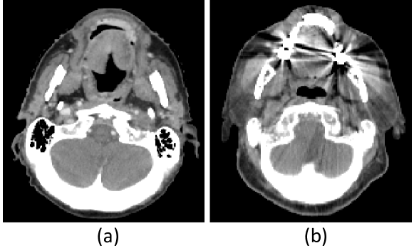
Figure 1: Representative clean (a) and noisy (b) slices.

3 Experiments

3.1 Data

We investigated the utility of kernel L²-Wasserstein distance to identify slices with dental artifacts in computerized tomography (CT) scans in head and neck cancer. Serious image degradation caused by metallic fillings or crowns in teeth is a common problem in CT images. We analyzed 1164 axial slices from 44 CT scans that were collected from 44 patients with head and cancer who were treated in our institution. This retrospective study was approved by the institutional review board and informed consent was obtained from all patients. Before the analysis, each CT slice was labeled as noisy or clean based on the presence of dental artifacts by a medical imaging expert, resulting in 276 noisy and 888 clean slices. Figure 1 shows representative noisy and clean CT slices from two different scans.

Table 1: GLCM-based 25 texture features used in this study.

No	Features	No	Features
1	Auto-correlation	14	Inverse Difference Moment
2	Joint Average	15	First Informal Correlation
3	Cluster Prominence	16	Second Informal Correlation
4	Cluster Shade	17	Inverse Difference Moment Normalized
5	Cluster Tendency	18	Inverse Difference Normalized
6	Contrast	19	Inverse Variance
7	Correlation	20	Sum Average
8	Difference Entropy	21	Sum Entropy
9	Dissimilarity	22	Sum Variance
10	Difference Variance	23	Haralick Correlation
11	Joint Energy	24	Joint Maximum
12	Joint Entropy	25	Joint Variance
13	Inverse Difference

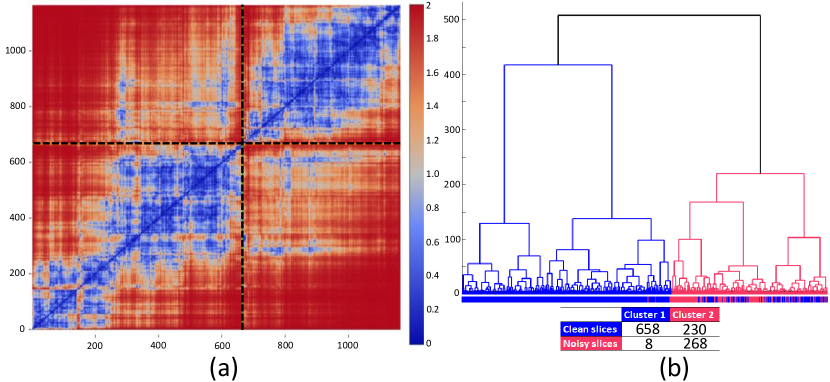
Figure 2: Results for kernel Wasserstein distance: (a) heatmap for the resulting distance matrix and (b) hierarchical clustering result conducted using the distance matrix.

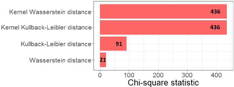
Figure 3: Chi-square statistics for four methods: Wasserstein, kernel Wasserstein, Kullback-Leibler, and kernel Kullback-Leibler distances.

3.2 Texture Features

Intensity thresholding (at the 5th percentile) was performed to exclude air voxels on each CT slice. The Computational Environment for Radiological Research (CERR) radiomics toolbox was then used to calculate the gray-level co-occurrence matrix (GLCM) from the remaining voxels using 64 gray levels and with a neighborhood of 8 voxels across all 4 directions in 2D [29, 30]. A total of 25 scalar features were then extracted from the GLCM (listed in Table 1). For further information on the GLCM features used, see https://github.com/cerr/CERR/wiki/Radiomics. Each feature was normalized between 0 and 1 for further analysis.

3.3 Experimental Results

For 1164 CT slices, we computed kernel Wasserstein distance between each pair of slices on 25 GLCM-based texture features. After that, we conducted unsupervised hierarchical clustering using the resulting distance matrix. Figure 2(a) shows a heatmap of the symmetric distance matrix for each pair of slices and Figure 2(b) presents the hierarchical clustering result. We identified two clusters: Cluster 1 with blue lines and Cluster 2 with red lines, consisting of 666 and 498 slices, respectively. In Figure (b), the bar under the hierarchical graph indicates the actual labels with blue for clean slices and red for noisy slices. As a result, Cluster 1 has 658 clean and 8 noisy slices whereas Cluster 2 has 230 clean and 268 noisy slices (table in Figure 2(b)). That is, Cluster 1 and 2 were significantly enriched for clean and noisy slices, respectively, with a Chi-square test p-value < 0.0001. Prediction rates were 97.10% and 74.10% for noisy and clean slices, respectively, and overall prediction rate was 79.6%. In Figure 2(a), the order of slices is the same as that shown in Figure 2(b) and the two clusters were divided by the black dot lines; the left bottom block represents Cluster 1 and the right top block for Cluster 2. The areas with blue color indicate close distance between slices whereas the areas with red color indicate far distance. Not surprisingly, the blue areas are mostly shown in the two blocks that represent the distances within each cluster. On the other hand, other two blocks (in the left top and right bottom) mostly have red areas, implying far distance between two clusters (between noisy and clean slices).

We compared performance of kernel Wasserstein distance with other methods, including Wasserstein, KL, and kernel KL distances, using Chi-square statistic. Note that for KL and kernel KL we computed the average value of two KL measures, i.e., $J_{\mathrm{KL}}(P\|Q)$. We repeated the analysis process noted above for alternative methods. Of note, kernel methods (kernel Wasserstein distance and kernel KL distance) had the same accuracy with a Chi-square statistic of 436 (Figure 3). By contrast, non-kernel methods (Wasserstein distance and KL distance) had substantially lower Chi-square statistics with 21 and 91, respectively, showing the superiority of kernel methods in this application.

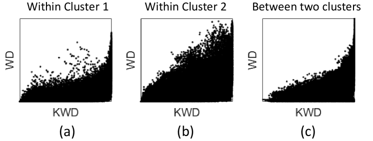
Figure 4 shows scatter plots for the correlation between kernel Wasserstein distance and Wasserstein distance in Cluster 1 (Figure 4(a)), Cluster 2 (Figure 4(b)), and between two clusters (Figure 4(c)). Compared to the correlation in Cluster 1 and between two clusters, the correlation in Cluster 2 that was enriched for noisy slices showed relatively more linear pattern. This may suggest that the impact of kernel Wasserstein distance in Cluster 1 and between two clusters is larger than classical Wasserstein distance, thereby leading to improved performance.

Figure 4: Scatter plots for the correlation between kernel Wasserstein distance and Wasserstein distance in (a) Cluster 1, (b) Cluster 2, and (c) between two clusters. KWD: kernel Wasserstein distance and WD: Wasserstein distance.

4 Conclusion

The Wasserstein distance is a powerful tool with a wide range of applications. Although extensively used, the method of computing this in the kernel space is lacking. In this paper, we proposed a computational method to solve L²-Wasserstein distance in the kernel space. We applied this method to a medical imaging problem in which CT scans are often degraded by artifacts arising from high-density materials. Our unsupervised method consisting of kernel L²-Wasserstein distance and hierarchical clustering showed a good level of performance in identifying noisy CT slices, outperforming conventional Wasserstein distance. Notably, kernel Kullback-Leibler distance also obtained comparable performance. This implies the nonlinearity of data and thus nonlinear analysis using kernel methods would be more likely to be essential. Future work will focus on further applications of kernel Wasserstein distance in imaging and biological data analysis.

Acknowledgments

This research was funded in part through National Institutes of Health/National Cancer Institute Cancer Center Support grant P30 CA008748.

References

• [1] Peyre G, Cuturi M: Computational Optimal Transport: With Applications to Data Science. Foundations and Trends(R) in Machine Learning 2019.
• [2] Chen Y, Cruz FD, Sandhu R, Kung AL, Mundi P, Deasy JO, Tannenbaum A: Pediatric sarcoma data forms a unique cluster measured via the earth mover’s distance. Scientific Reports 2017, 7:7035.
• [3] Chen Y, Georgiou TT, Tannenbaum A: Optimal transport for Gaussian mixture models. IEEE Access 2019, 7:6269–6278.
• [4] Luise G, Rudi A, Pontil M, Ciliberto C: Differential properties of sinkhorn approximation for learning with wasserstein distance. Advances in Neural Information Processing Systems 2018, :5864–5874.
• [5] Zhao X, Su Z, Gu X, Kaufman A, Sun J, Gao J, Luo F: Area-preservation mapping using optimal mass transport. IEEE Trans Vis Comput Graph. 2013, 19(12):2838–2847.
• [6] Evans LC: Partial Differential Equations and Monge-Kantorovich Mass Transfer. Current Developments in Mathematics 1999, 1997:65–126.
• [7] Villani C: Topics in optimal transportation. American Mathematical Soc. 2003.
• [8] Kantorovich L: On the translocation of masses, Dokl. Akad. Nauk SSSR 37 (1942) 227-229, English translation:. Journal of Mathematical Sciences 2006, 133:1381–1382.
• [9] Pouryahya M, Oh J, Javanmard P, Mathews J, Belkhatir Z, Deasy J, Tannenbaum AR: A Novel Integrative Multiomics Method Reveals a Hypoxia-Related Subgroup of Breast Cancer with Significantly Decreased Survival. bioRxiv 2019.
• [10] Mallasto A, Feragen A: Learning from uncertain curves: The 2-Wasserstein metric for Gaussian processes. Advances in Neural Information Processing Systems 2017, :5660–5670.
• [11] BAUDAT G, ANOUAR F: Generalized Discriminant Analysis Using a Kernel Approach. Neural Computation 2000, 12(10):2385–2404.
• [12] Oh J, Gao J: Fast kernel discriminant analysis for classification of liver cancer mass spectra. IEEE/ACM Trans Comput Biol Bioinform. 2009, 8(6):1522–1534.
• [13] Scholkopf B: The kernel trick for distances. Advances in Neural Information Processing Systems 2000, :301–307.
• [14] Rahimi A, Recht B: Random Features for Large-Scale Kernel Machines. Advances in Neural Information Processing Systems 2007, :1177–1184.
• [15] Oh J, Gao J: A kernel-based approach for detecting outliers of high-dimensional biological data. BMC Bioinformatics 2009, 10(Suppl 4):S7.
• [16] Masarotto V, Panaretos VM, Zemel Y: Procrustes Metrics on Covariance Operators and Optimal Transportation of Gaussian Processes. Sankhya A 2018, :1–42.
• [17] Dowson D, Landau B: The Frechet distance between multivariate normal distributions. Journal of Multivariate Analysis 1982, 12(3):450–455.
• [18] Olkin I, Pukelsheim F: The distance between two random vectors with given dispersion matrices. Linear Algebra and its Applications 1982, 48:257–263.
• [19] Malago L, Montrucchio L, Pistone G: Wasserstein Riemannian geometry of Gaussian densities. Information Geometry 2018, 1:137–179.
• [20] Hong Y, Horn RA: The Jordan cononical form of a product of a Hermitian and a positive semidefinite matrix. Linear Algebra and its Applications 1991, 147:373–386.
• [21] de Gosson M, Luef F: The Multi-Dimensional Hardy Uncertainty Principle and its Interpretation in Terms of the Wigner Distribution; Relation With the Notion of Symplectic Capacity. arXiv 2008.
• [22] Gretton A, Borgwardt KM, Rasch MJ, Scholkopf B, Smola A: A Kernel Two-Sample Test. Journal of Machine Learning Research 2012, 13:723–773.
• [23] Bauckhage C: Computing the Kullback-Leibler Divergence between two Weibull Distributions. arXiv 2013.
• [24] Ye J, Li T, Xiong T, Janardan R: Using uncorrelated discriminant analysis for tissue classification with gene expression data. IEEE/ACM Trans Comput Biol Bioinform. 2004, 1(4):181–190.
• [25] Li H, Zhang K, Jiang T: Robust and accurate cancer classification with gene expression profiling. IEEE Comput Syst Bioinform Conf. 2005, :310–321.
• [26] Ye J, Janardan R, Park C, Park H: An optimization criterion for generalized discriminant analysis on undersampled problems. IEEE Trans. Pattern Anal. Mach. Intell. 2004, 26(8):982–994.
• [27] Lai S, Vemuri B: Sherman-morrison-woodbury-formula-based algorithms for the surface smoothing problem. Linear Algebra and its Applications 1997, 265:203–229.
• [28] Rakocevic G, Djukic T, Filipovic N, Milutinovic V: Computational Medicine in Data Mining and Modeling. Springer New York 2013.
• [29] Apte A, Iyer A, Crispin-Ortuzar M, Pandya R, van Dijk L, Spezi E, Thor M, Um H, Veeraraghavan H, Oh J, Shukla-Dave A, Deasy J: Technical Note: Extension of CERR for computational radiomics: A comprehensive MATLAB platform for reproducible radiomics research. Med. Phys. 2018, 45(8):3713–3720.
• [30] Folkert M, Setton J, Apte A, Grkovski M, Young R, Schoder H, Thorstad W, Lee N, Deasy J, Oh J: Predictive modeling of outcomes following definitive chemoradiotherapy for oropharyngeal cancer based on FDG-PET image characteristics. Phys Med Biol. 2017, 62(13):5327–5343.