Detection of second-order topological superconductors by Josephson junctions

Abstract

We study Josephson junctions based on second-order topological superconductors (SOTSs) which can be realized in quantum spin Hall insulators with large inverted gap in proximity to unconventional superconductors. We find that tuning the chemical potential in the superconductor strongly modifies the induced pairing of the helical edge states, resulting in topological phase transitions. In a corresponding Josephson junction, a $0$-$\pi$ transition is realized by tuning the chemical potentials in the superconducting leads. This striking feature is stable in junctions with respect to different sizes, doping the normal region, and the presence of disorder. Our transport results can serve as novel experimental signatures of SOTSs. Moreover, the $0$-$\pi$ transition constitutes a fully electric way to create or annihilate Majorana bound states in the junction without any magnetic manipulation.

Introduction.–The second-order topological superconductor (SOTS) is a novel topological phase of matter and features Majorana zero-dimensional (0D) corner or 1D hinge states which are two spatial dimensions lower than the gapped bulk (Langbehn et al., 2017; Khalaf, 2018; Wang et al., 2018a; Yan et al., 2018; Liu et al., 2018; Geier et al., 2018; Zhu, 2018; Hsu et al., 2018; Wang et al., 2018; Zhang et al., 2019a; Qin et al., ; Bultinck et al., 2019; Peng et al., 2019). They may form stable qubits for topological quantum computation (Kitaev, 2001, 2003; Nayak et al., 2008; Alicea, 2012; Leijnse and Flensberg, 2012; Beenakker, 2013; Elliott and Franz, 2015; Sarma et al., 2015; Sato and Fujimoto, 2016). Recently, the SOTS has been discovered in a variety of realistic materials and triggered tremendous interest (Wang et al., 2018a; Yan et al., 2018; Liu et al., 2018; Geier et al., 2018; Qin et al., ; König and Coleman, ; Zhu, 2018; Hsu et al., 2018; Volpez et al., 2019; Wang et al., 2018; Zhang et al., 2019a; Shapourian et al., 2018; Pan et al., ; Kheirkhah et al., ; Ghorashi et al., ). One way to mimic SOTSs in 2D is given by quantum spin Hall insulators (QSHIs) in proximity to unconventional superconductors with $d_{x^{2}-y^{2}}$-wave or $s_{\pm}$-wave pairing order (Wang et al., 2018a; Yan et al., 2018; Liu et al., 2018). The proximity effect of unconventional superconductivity in 2D systems has been intensively explored in theory (Linder and Sudbø, 2008; Linder et al., 2010; Black-Schaffer and Balatsky, 2013; Zhang et al., 2013; Li et al., 2015; Zareapour et al., 2016; Li et al., 2016; Wu et al., 2016; Wang et al., 2015; Zhou et al., 2019) and experiment (Zareapour et al., 2012; Wang et al., 2013; Zhao et al., 2018; Perconte et al., 2018; Xu et al., 2014; Yilmaz et al., 2014). To date, however, the only way proposed to detect 2D SOTSs is a tunneling experiment without a concrete calculation of the observable signature. An alternative approach to probe SOTSs and manipulate the Majorana corner modes is thus needed. In QSHIs, a finite doping is typically present, and the chemical potential can be far away from the Dirac points. Therefore, it is certainly interesting and experimentally relevant to explore the influence of the chemical potential in SOTSs.

In this Letter, we investigate superconductor-normal metal-superconductor (SNS) junctions formed by a 2D SOTS. The SOTS can be realized in a QSHI with a large inverted gap in proximity to an unconventional superconductor. We introduce a minimal model which is able to capture the essential physics of the SOTS. We find that due to the nontrivial momentum-dependence of the pairing potential and mass, the chemical potential in the SOTS alters the pairing gap opened within the edge states significantly. It can even switch the sign of the pairing gap, leading to a topological phase transition. While the supercurrent across the SNS junction is insensitive to the chemical potential in the N region, it depends strongly on the filling in the superconductors. Strikingly, tuning the chemical potentials in the superconductors gives rise to a $0$-$\pi$ transition, which is absent in junctions based on conventional $s$-wave pairing. These features are robust against disorder in junctions with different sizes. They offer novel signatures to detect the SOTS with Majorana corner states. Furthermore, while Majorana bound states (MBSs) emerge in the $0$-junction when the phase difference across the junction is $\phi=\pm\pi$, they appear at vanishing $\phi$ in the $\pi$-junction. Thus, Josephson junctions with such a doping-induced $0$-$\pi$ transition provide an innovative platform to create or annihilate MBSs by electric gating in the absence of $\phi$. These predictions are applicable to a number of candidate systems including high-temperature QSHIs (Qian et al., 2014; Tang et al., 2017; Fei et al., 2017; Wu et al., 2018; Chen et al., 2018; Weng et al., 2015; Si et al., 2016; Reis et al., 2017; Hsu et al., 2015; Wrasse and Schmidt, 2014; Liu et al., 2015; Wan et al., 2017) in proximity to high-temperature cuprate or iron-based superconductors.

Minimal model for SOTSs.–We consider the minimal model for SOTSs realized in QSHIs in proximity to superconductors,

$$H({\bf k}) = H_{0}({\bf k})+\Delta({\bf k})\tau_{y}s_{y},$$

$$H_{0}({\bf k}) = m({\bf k})\tau_{z}\sigma_{z}+v_{x}k_{x}s_{z}\sigma_{x}+v_{y}k_{y}\tau_{z}\sigma_{y}-\mu\tau_{z}$$ (1)

written in the Nambu basis $(c_{a,\uparrow,{\bf k}},c_{b,\uparrow,{\bf k}},c_{a,\downarrow,{\bf k}},c_{b,\downarrow,{\bf k}},$ $c_{a,\uparrow,-{\bf k}}^{\dagger},c_{b,\uparrow,-{\bf k}}^{\dagger},c_{a,\downarrow,-{\bf k}}^{\dagger},c_{b,\downarrow,-{\bf k}}^{\dagger})$, where $c_{\sigma,s,{\bf k}}^{\dagger}$($c_{\sigma,s,{\bf k}}$) creates(annihilates) an electron with spin $s\in\{\uparrow,\downarrow\}$, orbital $\sigma\in\{a,b\}$ and the momentum ${\bf k}=(k_{x},k_{y})$ measured from the band inversion point of the QSHI. $\bm{\tau}$, $\bm{\sigma}$ and $\bm{s}$ are Pauli matrices acting on Nambu, orbital and spin spaces, respectively. $m({\bf k})=m_{0}-m_{x}k_{x}^{2}-m_{y}k_{y}^{2}$ is the mass term of the QSHI and $\mu$ is the chemical potential. The band inversion implies the conditions $m_{0}m_{x}>0$ and $m_{0}m_{y}>0$ (Bernevig et al., 2006). The pairing potential is written in general as $\Delta({\bf k})=\Delta_{0}+\Delta_{2}\left(k_{x}^{2}-k_{y}^{2}\right)$. When $\Delta_{0}\neq 0$ and $\Delta_{2}=0$, it refers to conventional $s$-wave pairing. When $\Delta_{0}=0$ and $\Delta_{2}\neq 0$, the pairing is formally $d_{x^{2}-y^{2}}$-wave. It can be induced in a QSHI with band inversion at the $\Gamma$ point via the proximity to a cuprate superconductor (Yan et al., 2018). When $0\leqslant|\Delta_{0}|<m_{0}|\Delta_{2}|/2m_{x(y)}$, the system possesses a mixture of $s$-wave and $d_{x^{2}-y^{2}}$-wave pairing. It can also describe effectively a QSHI with band inversion at the $X$ point (Wan et al., 2017; Wrasse and Schmidt, 2014; Liu et al., 2015) and $s_{\pm}$-wave pairing induced from an iron-based superconductor (Stewart, 2011; Hirschfeld et al., 2011; Zhang et al., 2018; Wang et al., 2018b; Zhang et al., 2019b).

In the absence of $\Delta({\bf k})$, the system hosts gapless helical edge states across the bulk gap, which are protected by time-reversal symmetry. The pairing term with $\Delta_{2}\neq 0$ induces a pairing gap of the edge states. The gap may switch sign at the corners, resulting in Majorana corner modes (Yan et al., 2018; Wang et al., 2018a; Liu et al., 2018). We note that although the model (1) is a low-energy effective model, it captures the essential physics of the SOTS. Based on this model, we can understand the second-order topology more intuitively from the picture of edge states and show that it can be strongly altered by changing $\mu$.

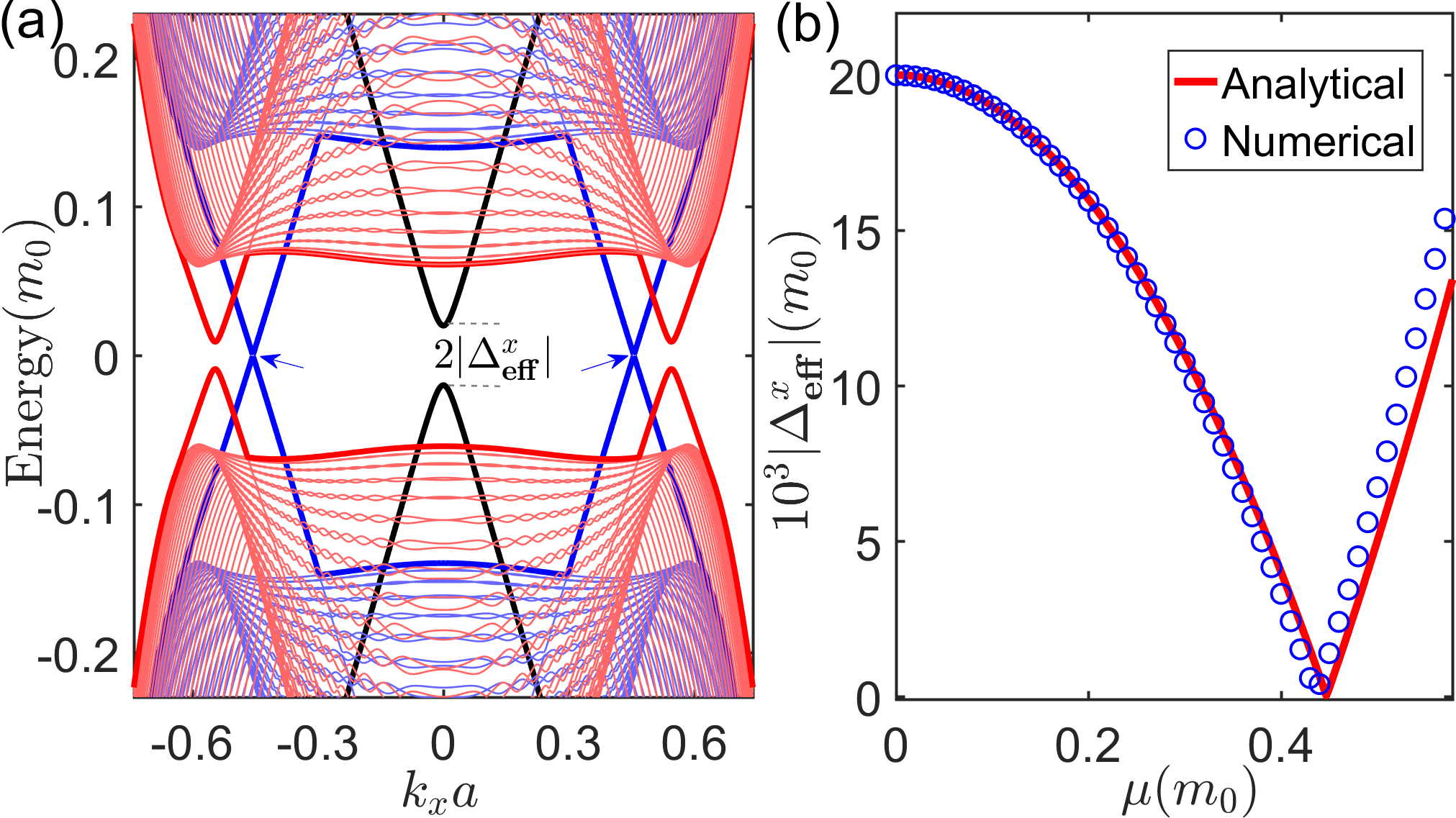
Fig. 1: (a) Energy spectra of the model (1) in a ribbon along $x$ direction for chemical potential $\mu=0$ (black), $0.44m_{0}$ (blue), and $0.52m_{0}$ (red), respectively. The thick curves close to zero energy are edge bands. The pairing gap $\Delta_{\text{eff}}^{x}$ vanishes at around $\mu=0.44m_{0}$, as pointed by the blue arrows. (b) $|\Delta_{\text{eff}}^{x}|$ as a function of $\mu$. The blue circles are numerical results from tight-binding calculation while the red curve is the plot of Eq. (5). Other parameters are $m_{x(y)}=2.5,$ $v_{x(y)}=1,$ $\Delta_{0}=0,$ $\Delta_{2}=0.05$ and $200$ lattice layers in $y$ direction. The units for energy and wavenumber are $m_{0}$ and $a^{-1}$, respectively.

Pairing gaps of edge states and topological phase transitions.–To analyze the Majorana corner states and the influence of $\mu$ on the SOTS, we analytically derive the effective model for edge states. For illustration, we consider the edge along $x$ direction of the SOTS in the half-plane $y\leqslant 0$ and assume hard-wall boundary conditions (Note, 5). As in realistic systems, we assume weak pairing. We first calculate the edge states of $H_{0}$, following the approach of Ref. (Zhang et al., 2016). In this model, $k_{x}$ is a good quantum number. The helical electron and hole edge bands are found explicitly as

$$E_{e(h),\uparrow/\downarrow}(k_{x})=\pm\text{sgn}(m_{y}v_{y})v_{x}k_{x}-(+)\mu.$$ (2)

The wavefunctions in the orbital basis $\{a,b\}$ read

$$\Psi_{e,\uparrow,k_{x}}({\bf r})=\mathcal{N}e^{ik_{x}x}(e^{\lambda_{1}y}-e^{\lambda_{2}y})\left(\text{sgn}(m_{y}v_{y}),1\right)^{T}.$$ (3)

They fulfill $\Psi_{e,\downarrow,k_{x}}({\bf r})=\Psi_{e,\uparrow,-k_{x}}^{*}({\bf r})$ and $\Psi_{h,\downarrow/\uparrow,k_{x}}({\bf r})=\Psi_{e,\downarrow/\uparrow,-k_{x}}^{*}({\bf r})$, due to time-reversal and particle-hole symmetries; $\lambda_{1(2)}=|v_{y}/2m_{y}|-(+)(v_{y}^{2}/4m_{y}^{2}-m_{0}/m_{y}+m_{x}k_{x}^{2}/m_{y})^{1/2}$ and $\mathcal{N}$ is the normalization factor. The decaying length of edge states is given by $\xi_{\text{edge}}=\text{max}[1/\text{Re}(\lambda_{1}),1/\text{Re}(\lambda_{2})]$. At zero energy, the electron and hole bands touch at $k_{x}=\pm k_{c}$ with $k_{c}=\text{sgn}(m_{y}v_{y})$ $\mu/v_{x}$. For $\mu=0$, $k_{c}=0$. However, for $\mu\neq 0$, the touching points shift to finite $\pm k_{c}$. Projecting the pairing term onto the edge states, the resulting Bogoliubov de-Gennes (BdG) Hamiltonian for edge states is obtained as

$$h_{\text{BdG}}^{x}=\text{sgn}(m_{y}v_{y})v_{x}k_{x}\tau_{z}s_{z}-\mu\tau_{z}+\Delta_{\text{eff}}^{x}\tau_{x}s_{z}$$ (4)

in the basis $(\Psi_{e,\uparrow},\Psi_{e,\downarrow},\Psi_{h,\downarrow},\Psi_{h,\uparrow})$, and the pairing gap is given by

$$\Delta_{\text{eff}}^{x}=-\Delta_{0}+\Delta_{2}\left[m_{0}/m_{y}-(1+m_{x}/m_{y})\mu^{2}/v_{x}^{2}\right].$$ (5)

Without loss of generality, a real $\Delta({\bf k})$ has been assumed (Note, 1). We provide the derivation in detail in the Supplemental Material (Sup, ). Similarly, for an edge along $y$ direction, we find the BdG Hamiltonian of the same form but with a different pairing gap

$$\Delta_{\text{eff}}^{y}=-\Delta_{0}-\Delta_{2}\left[m_{0}/m_{x}-(1+m_{y}/m_{x})\mu^{2}/v_{y}^{2}\right].$$ (6)

The combination of $\Delta_{\text{eff}}^{x}$ and $\Delta_{\text{eff}}^{y}$ (with opposite signs) in Eq. (4) mimics the Jackiw-Rebbi model (Jackiw and Rebbi, 1976) at corners of $x$ and $y$ axes. Thus, Majorana corner states at zero energy appear if $\Delta_{\text{eff}}^{x}\Delta_{\text{eff}}^{y}<0$.

For $s$-wave pairing, $\Delta_{\text{eff}}^{x}$ and $\Delta_{\text{eff}}^{y}$ are identical and constant. Thus, no corner state emerge. In contrast, for unconventional pairings with $|\Delta_{0}|<m_{0}|\Delta_{2}|/2m_{x(y)}$, we obtain corner states at small $\mu$. When $\mu=0$, the SOTS has two reflection symmetries. When $m_{x}=m_{y}$, $v_{x}=v_{y}$ and $\Delta_{0}=0$, it possesses a fourfold rotation symmetry. In these particular cases, the system can be characterized by a topological invariant calculated from the bulk Hamiltonian (Benalcazar et al., 2017a, b; Song et al., 2017; Sup, ). However, the corner states in our model are not restricted to any crystalline symmetries. Interestingly, $\Delta_{\text{eff}}^{x(y)}$ depends strongly on $\mu$. The $\mu$ dependence stems from the quadratic terms in the model (1), which are crucial for the topological properties of the SOTS. Moreover, $\Delta_{\text{eff}}^{x(y)}$ vanishes at $\mu=\pm\mu_{x(y)}^{c}$, where

$$\mu_{x(y)}^{c}=|v_{x(y)}|\sqrt{[m_{0}/m_{y(x)}\mp\Delta_{0}/\Delta_{2}]/(1+m_{x(y)}/m_{y(x)})}.$$ (7)

This behavior indicates that we can switch the sign of $\Delta_{\text{eff}}^{x(y)}$ by varying $\mu$. Without loss of generality, we suppose $\mu_{x}^{c}\leqslant\mu_{y}^{c}$. The system is in a SOTS phase in the parameter regions $0\leqslant|\mu|<\mu_{x}^{c}$ and $\mu_{y}^{c}<|\mu|<m_{\text{g}}$ with $m_{\text{g}}$ being the bulk gap Note (2), whereas if $\mu_{x}^{c}<|\mu|<\mu_{y}^{c}$, it becomes a trivial superconductor with no corner state. For the particular case with $v_{x(y)}=v$, $m_{x(y)}=m$, and $\Delta_{0}=0$, $\Delta_{\text{eff}}^{x}$ and $\Delta_{\text{eff}}^{y}$ are always opposite. They both close at $\mu=\pm v\sqrt{m_{0}/2m}$. Thus, there is no parameter space for the trivial phase. Nevertheless, the sign of $\Delta_{\text{eff}}^{x(y)}$ can still be changed by a finite $\mu$ inside the bulk gap (Note, 3) if

$$2m_{0}m>v^{2}.$$ (8)

This condition indeed corresponds to a QSHI phase with a large inverted gap or equivalently an indirect bulk gap. It is likely realized in the inverted InAs/GaSb bilayer (Liu et al., 2008; Knez et al., 2011; Krishtopenko and Teppe, 2018), WTe₂ monolayer (Qian et al., 2014; Tang et al., 2017; Fei et al., 2017; Wu et al., 2018; Chen et al., 2018), functionalized MXene (Weng et al., 2015; Si et al., 2016), Bismuthene on SiC (Reis et al., 2017; Hsu et al., 2015), and PbS monolayer (Wan et al., 2017; Wrasse and Schmidt, 2014; Liu et al., 2015).

To test our analytical results, we discretize the model (1), put it on a square lattice, choose a proper set of parameters (satisfying the inequality (8)) and calculate the energy spectrum in a ribbon geometry (Note, 6). For concreteness, we consider $\Delta_{0}=0$ and set the lattice constant $a$ to unity. As shown in Fig. 1(a), the edge states for $\mu=0$ open a gap at $k_{x}=0$. As $\mu$ is increased, the gap splits to two points away from $k_{x}=0$. The magnitude of the gap first decreases, vanishes at a critical $\mu$ and then reopens, which explicitly demonstrates a topological phase transition. This behavior is in perfect agreement with Eq. (5), cf. Fig. 1(b).

0-$\pi$ transition and its robustness.–We now consider an SNS junction in which two SOTSs (also called S leads below) are connected by a QSHI with length $L$ in $x$ direction, as sketched in Fig. 2(a). The width of the junction ribbon is $W$. For simplicity, we assume the chemical and pairing potentials in step-like forms. $\mu_{L(R)}$ and $\mu_{N}$ denote the chemical potentials in the left(right) S lead and N (QSHI) region, respectively. $\phi$ is the phase difference across the junction. We calculate the supercurrent $J_{s}$ by the lattice Green’s function technique (Asano, 2001; Martín-Rodero et al., 1994; Furusaki, 1994) and provide the details in the Supplemental Material (Sup, ).

At low temperatures, the transport in the junction is conducted dominantly by helical edge channels. Perfect Andreev reflection occurs at the NS interfaces. Thus, the current-phase relation (CPR) takes a sawtooth shape with a sudden jump, see Fig. 2(b). The sawtooth-like CPR is insensitive to $\mu_{N}$ and stays stable in junctions of different sizes ($L$ and $W$), provided that the two edges at $y=\pm W/2$ are well separated, $W\gg\xi_{\text{edge}}$. The sudden jump can be related to the fermion parity anomaly at each edge (Fu and Kane, 2009; Crépin and Trauzettel, 2014). It indicates the formation of degenerate MBSs in the junction discussed below. $J_{s}$ decreases monotonically with increasing $L$, see Fig. 2(b). The critical current $J_{c}$ (maximal value of $J_{s}$) decays as $\text{$\sim$}1/L$ in long junctions, similar to junctions based on conventional s-wave pairing. In short junctions, $J_{c}$ is of the same order of magnitude but always smaller than $e\sqrt{|\Delta_{L}\Delta_{R}|}/\hbar$, in contrast to the case of $s$-wave pairing. In this estimate, $\Delta_{L(R)}$ is the induced pairing gap of edge states in the left(right) S lead and determined by Eq. (5). We attribute this difference to the inhomogeneity of the superconducting pairing at the boundaries of our setup.

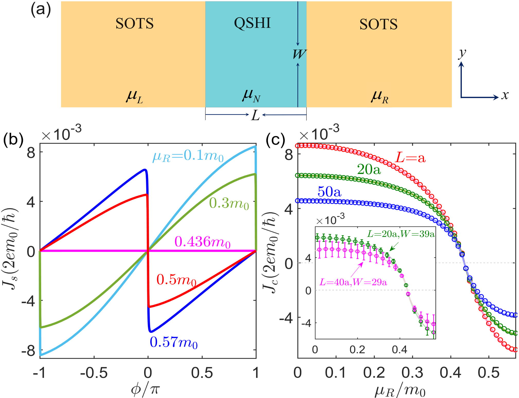
Fig. 2: (a) Schematic for the SNS setup; (b) Current-phase relations for $L=a$ and $\mu_{R}=0.1m_{0}$, $0.3m_{0},$ $0.436m_{0},$ $0.5m_{0}$ and $0.57m_{0}$, respectively. (b) Critical current $J_{c}$ as a function of $\mu_{R}$ for $L=a$ (red), $20a$ (green) and $50a$ (blue), respectively. The inset displays the results in the presence of disorder of strength $V_{\text{dis}}=m_{0}$ for $W=39a$ and $L=20a$ (green), $W=29a$ and $L=40a$ (purple), respectively. The error bars are $500$ times enlarged for visibility. For all solid curves, $\mu_{L}=\mu_{N}=0.1m_{0}$, $W=39a$, $k_{B}T=10^{-3}\Delta_{L}$ and other parameters are the same as those in Fig. 1. The circled dots in (c) are the same as the solid curves but for $\mu_{N}=-0.3m_{0}$.

The CPRs for a fixed $\mu_{L}$ and various values of $\mu_{R}$ are displayed in Fig. 2(a). Since $J_{s}$ is even in $\mu_{L(R)}$, we present only the results for $\mu_{L(R)}>0$. While $J_{s}$ is insensitive to $\mu_{N}$, it decreases significantly when we increase $\mu_{R}$. This behavior can be understood as a result of the reduction of $|\Delta_{R}|$ by $\mu_{R}$, see Eq. (5). Strikingly, increasing $\mu_{R}$ further, we observe a clear $0$-$\pi$ transition for the parameters satisfying the inequality (8). While $J_{s}(\phi)$ in the region $0<\phi<\pi$ is positive for $\mu_{R}<\mu^{c}$, it becomes negative for $\mu_{R}>\mu^{c}$. We coin the former case a $0$-junction and the latter one a $\pi$-junction. Meanwhile, the sudden jump of the CPR is switched to $\phi=0$ in the $\pi$-junction, which is in strong contrast to the $0$-junction where the jump is at $\phi=\pm\pi$. In Fig. 2(c), we plot $J_{c}$ as a function of $\mu_{R}$. The critical value $\mu^{c}$ for the transition is approximately given by $v\sqrt{m_{0}/2m}$, in accord with our analytical result. Close to $\mu^{c}$, $J_{c}$ drops quickly and switches sign. These features are generic and apply to junctions of different lengths and widths. They are also robust with respect to nonmagnetic disorder in the N region. To illustrate this, we model the disorder as random on-site potentials in the range $[-V_{\text{dis}}/2,V_{\text{dis}}/2]$ (Li et al., 2018; Sup, ) and calculate 200 random disorder configurations in the inset of Fig. 2(c). There is no qualitative difference in the features compared to those in clean junctions. This can be expected since the helical edge channels which mediate the transport are less sensitive to backscattering. Similar effects can be observed by tuning $\mu_{L}$ and fixing $\mu_{R}$. Finally, it is important to note that the variation of $J_{s}$ and the $0$-$\pi$ transition by tuning $\mu_{L(R)}$ are directly related to the strong $\mu_{L(R)}$-dependence in $\Delta_{L(R)}$ in the SOTS, and absent in conventional junctions based on $s$-wave pairing.

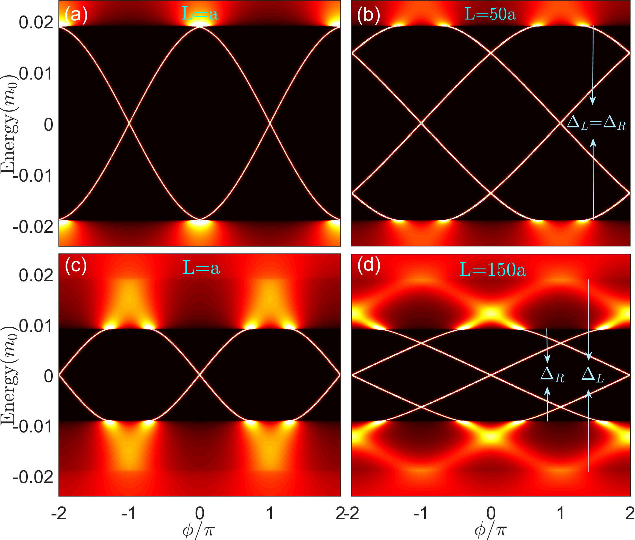
Fig. 3: Andreev bound states for $\mu_{R}=0.1m_{0}$ (a,b) and $\mu_{R}=0.52m_{0}$ (c,d), respectively. (a,c) are for short junctions with $L=a$, while (b,d) for long junctions with $L=50a$ and $150a$, respectively. For all plots, $W=39a$ and other parameters are the same as those in Fig. 1.

Majorana bound states.–Next, we discuss the Andreev bound states (ABSs) formed in the junction, which can be obtained from the lattice Green’s function. In short junctions, there are two bands of ABSs with opposite energies, see Fig. 3(a,c). When the sudden jump of the CPR occurs, the positive and negative bands touch at zero energy. This degeneracy is robust and protected by time-reversal and particle-hole symmetries. It resembles Kramers pairs of MBSs. This can be best understood from the effective Hamiltonian (4) for edge states. In the short junction limit, two ABS bands at a given edge can be described by

$$E_{\pm}(\phi)=\pm\dfrac{\Delta_{L}\Delta_{R}\sin\phi}{\sqrt{\Delta_{L}^{2}+\Delta_{R}^{2}-2\Delta_{L}\Delta_{R}\cos\phi}}.$$ (9)

Notably, the ABSs are confined in the pairing gaps for $\phi$ satisfying $(\cos\phi$$-$$\Delta_{L}/\Delta_{R})(\cos\phi$$-$$\Delta_{R}/\Delta_{L})>0$, as verified in Fig. 3(a,c). Noticing $\Delta_{L}\Delta_{R}>0$ in the $0$-junction for $\mu_{R}<\mu^{c}$, whereas $\Delta_{L}\Delta_{R}<0$ in the $\pi$-junction for $\mu_{R}>\mu^{c}$, we can see that $E_{\pm}(\phi)$ touch at $\phi=\pm\pi$ and $0$, respectively. Using the valid formula at zero temperature, $J_{s}(\phi)=\partial|E_{+}(\phi)|/\partial\phi$ (Beenakker, 1991), we also reproduce the sudden jump in the CPR. The wavefunctions of the zero modes can be written as

$$\gamma_{+}(x) = \Psi_{+}\eta(x)+\Psi_{-}\eta^{*}(x)$$

$$\gamma_{-}(x) = i\Psi_{+}\eta(x)-i\Psi_{-}\eta^{*}(x),$$ (10)

where $\Psi_{\pm}=\text{sgn}(\Delta_{L})\Psi_{h/e,\downarrow}\mp i\Psi_{e/h,\uparrow}$ and the spatial dependence is $\eta(x)=\exp\{[\theta(x)(i\mu_{R}$$-$$|\Delta_{R}|)+\theta(-x)(i\mu_{L}+|\Delta_{L}|)]x/v\}$ (Sup, ). Since $\Psi_{h,\downarrow/\uparrow}=\Psi_{e,\downarrow/\uparrow}^{*}$, the zero modes have self-adjoint wavefunctions, $\gamma_{\pm}(x)=\gamma_{\pm}^{*}(x)$. They are Majorana fermions. Under the time-reversal operation $\mathcal{T}$, $\mathcal{T}\Psi_{e,\downarrow/\uparrow}=\pm\Psi_{e\uparrow/\downarrow}^{*}$ and $\mathcal{T}\Psi_{h,\downarrow/\uparrow}=\pm\Psi_{h,\uparrow/\downarrow}^{*}$. Therefore, $\gamma_{\pm}$ are related by time-reversal symmetry, $\mathcal{T}\gamma_{+}=\gamma_{-}$. A similar analysis can be applied to the other edge where another Kramers pair of MBSs are located. In long junctions, all the features persist but with more pairs of discrete ABS bands emerging from the continuum spectrum, see Fig. 3(b,d).

At $\phi=0$, the MBSs emerge for $\mu>\mu^{c}$, whereas they disappear for $\mu<\mu^{c}$. In this sense, we are able to switch between the presence and absence of MBSs by gating the S leads in the absence of $\phi$. Our setup indeed realizes fully electrically controllable MBSs without fine tuning of magnetic field or threaded flux. This is an important advantage compared to previous proposals based on conventional $s$-wave superconductivity (Fu and Kane, 2008, 2009; Lutchyn et al., 2010; Sau et al., 2010; Oreg et al., 2010; Volpez et al., 2019). Moreover, since the localization lengths of the MBSs in the S leads are determined by $\xi_{L(R)}=|v/\Delta_{L(R)}|$, we are also able to control the spatial profiles of the MBSs by $\mu_{L(R)}$.

Experimental relevance and summary.–Now we briefly discuss the experimental relevance of our proposal. QSHIs with large inverted gaps (Qian et al., 2014; Tang et al., 2017; Fei et al., 2017; Wu et al., 2018; Chen et al., 2018; Weng et al., 2015; Si et al., 2016; Reis et al., 2017; Hsu et al., 2015; Wrasse and Schmidt, 2014; Liu et al., 2015; Wan et al., 2017; Liu et al., 2008; Knez et al., 2011; Krishtopenko and Teppe, 2018) in proximity to cuprate or iron-based superconductors (Stewart, 2011; Hirschfeld et al., 2011; Zhang et al., 2018; Wang et al., 2018b; Zhao et al., 2018; Zareapour et al., 2012; Wang et al., 2013; Zhang et al., 2019b) could provide promising platforms to verify our predictions. For concreteness, we take the inverted InAs/GaSb bilayer and WTe₂ monolayer to estimate $\mu_{x(y)}^{c}$. For simplicity, we consider $\Delta_{0}=0$ such that $\mu^{c}_{x}(y)$ is independent of the magnitude of the pairing potential. For the inverted InAs/GaSb bilayer, $m_{0}=0.0055$ eV, $m_{x(y)}=81.9$ eV$\cdot\mathring{\text{A}}$², $v_{x(y)}=0.72$ eV$\cdot\mathring{\text{A}}$ (Liu and Zhang, 2013). To realize the $0$-$\pi$ transition, one can fabricate the Josephson junction in any direction and find that $\mu_{x(y)}^{c}=0.0042$ eV which is smaller than the bulk gap $m_{\text{gap}}=0.005$ eV. For the WTe₂ monolayer with $m_{0}=0.33$ eV, $m_{x}=4.6$ eV$\cdot\mathring{\text{A}}{}^{2}$, $m_{y}=16.9$ eV$\cdot\mathring{\text{A}}$², $v_{x}=2.55$ eV$\cdot\mathring{\text{A}}$ and $v_{y}=0.3$ eV$\cdot\mathring{\text{A}}$ (Qian et al., 2014), we have $\mu_{x}^{c}=0.252$ eV, $\mu_{y}^{c}=0.057$ eV and $m_{\text{gap}}=0.08$ eV. Thus, it is better to design the junction in $y$ direction in our model (Note, 7). According to Eq. (7), the inclusion of a small $\Delta_{0}$ would suppress $\mu_{x}^{c}$ or $\mu_{y}^{c}$ and hence make it more feasible to observe the $0$-$\pi$ transition. A particle-hole symmetry breaking term, which is neglected here, breaks the symmetry with respect to $\mu$ but does not qualitatively change our main results.

We note in passing that there have been experimental efforts trying to incorporate unconventional superconductivity in topological systems (Zareapour et al., 2012; Wang et al., 2013; Zhao et al., 2018; Zhang et al., 2018; Wang et al., 2018b; Zhang et al., 2019b). Moreover, large proximity-induced pairing gaps in 2D systems from unconventional superconductors have been probed (Zareapour et al., 2012; Wang et al., 2013; Zhao et al., 2018; Perconte et al., 2018).

In summary, we have found that the chemical potentials in superconductors can be used to modulate the supercurrent and realize a $0$-$\pi$ transition in Josephson junctions based on SOTSs. These features are attributed to the dependence of the pairing gap of edge states on the chemical potential. They could serve as novel experimental signatures of the SOTS. We have predicted the $0$-$\pi$ transition as a fully electric way to create or annihilate MBSs at elevated temperatures.

Appendix A Derivation of the effective BdG model for edge states

A.1 Edges in $x$ or $y$ direction

In the absence of the pairing potential, the Bogoliubov-de Gennes (BdG) Hamiltonian [Eq. (1) in the main text] decouples into four blocks. Each block can be analyzed separately. Let us take the block for spin-up electrons for illustration, following the approach of Ref. (Zhang et al., 2016). The block for spin-up electrons reads

$$h_{e,\uparrow}({\bf k}) = \begin{pmatrix}m({\bf k})-\mu&v_{x}k_{x}-iv_{y}k_{y}\\ v_{x}k_{x}+iv_{y}k_{y}&-m({\bf k})-\mu\end{pmatrix}$$ (11)

in the basis $(c_{a,\uparrow},c_{b,\uparrow})$, where $m({\bf k})=m_{0}-m_{x}k_{x}^{2}-m_{y}k_{y}^{2}$.

Consider the edge in $x$ direction of a semi-infinite SOTS in the half-plane $y\leqslant 0$ and impose hard-wall boundary conditions. Then, $k_{x}$ is a good quantum number. We assume the trial wavefunction of the form,

$$\Psi_{\lambda}({\bf r}) = e^{ik_{x}x}e^{\lambda y}\psi_{\lambda},$$ (12)

where $\psi_{\lambda}$ is a two-component spinor. Plugging Eq. (12) in $h_{e,\uparrow}(-i\nabla_{{\bf r}})\Psi_{\lambda}=E\Psi_{\lambda}$, we obtain the secular equation

$$\det|h_{e,\uparrow}(k_{x},-i\lambda)-E-\mu| = 0$$ (13)

for a nontrivial solution of $\psi_{\lambda}$. Solving Eq. (13) gives four $\lambda$, denoted as $\beta\lambda_{\alpha}$ with $\beta=\pm$ and $\alpha=1,2$,

$$\lambda_{\alpha}^{2} = (-1)^{\alpha}\sqrt{v_{y}^{4}-4m_{y}^{2}[v_{y}^{2}m_{k}+v_{x}^{2}k_{x}^{2}+(E+\mu)^{2}]}/2m_{y}^{2}$$ (14)

$$+v_{y}^{2}/2m_{y}^{2}-m_{k},$$

where $m_{k}=(m_{0}-m_{x}k_{x}^{2})/m_{y}.$ Each $\beta\lambda_{\alpha}$ corresponds to a spinor state written as

$$\psi_{\alpha\beta} = \begin{pmatrix}m_{y}(m_{k}+\lambda_{\alpha}^{2})+E+\mu\\ v_{x}k_{x}+v_{y}\beta\lambda_{\alpha}\end{pmatrix},$$ (15)

or alternatively,

$$\psi_{\alpha\beta} = \begin{pmatrix}-v_{x}k_{x}+v_{y}\beta\lambda_{\alpha}\\ m_{y}(m_{k}+\lambda_{\alpha}^{2})-E-\mu\end{pmatrix}.$$ (16)

Then, a general wavefunction is given by

$$\Psi_{e,\uparrow,k_{x}}(E,{\bf r}) = e^{ik_{x}x}\sum_{\alpha=1,2}\sum_{\beta=\pm}C_{\alpha\beta}\psi_{\alpha\beta}e^{\beta\lambda_{\alpha}y},$$ (17)

where the energy $E$ and coefficients $C_{\alpha\beta}$ are found from the boundary conditions. The hard-wall boundary conditions read

$$\Psi_{e,\uparrow,k_{x}}(y = -\infty)=\Psi_{e,\uparrow,k_{x}}(y=0)=0.$$ (18)

The condition $\Psi_{e,\uparrow,k_{x}}(y=-\infty)=0$ requires that $\Psi_{e,\uparrow,k_{x}}$ contains only the terms with $\beta=+$ and $\mathrm{Re}(\lambda_{\alpha})>0$, i.e, $C_{1-}=C_{2,-}=0$. The other condition $\Psi_{e,\uparrow,k_{x}}(y=0)=0$ then leads to

$$\begin{vmatrix}(\psi_{1+}&\psi_{2+})\end{vmatrix} = 0.$$ (19)

Plugging Eqs. (15) and (16) into Eq. (19), respectively, and considering $\lambda_{1}\neq\lambda_{2}$, we obtain

$$E+\mu= v_{x} m_{y}k_{x}\left(\lambda_{1}+\lambda_{2}\right)/v_{y}-m_{y}\left(m_{k}-\lambda_{1}\lambda_{2}\right),$$

$$E+\mu= v_{x} m_{y}k_{x}\left(\lambda_{1}+\lambda_{2}\right)/v_{y}+m_{y}\left(m_{k}-\lambda_{1}\lambda_{2}\right).$$ (20)

By comparing these two equations, we identify

$$\lambda_{1}\lambda_{2} = m_{k}.$$ (21)

According to Eq. (14), there are two cases of $\lambda_{1,2}$, one is $\lambda_{1(2)}>0$ and the other $\lambda_{1}=\lambda_{2}^{*}$. In both cases, $\lambda_{1}\lambda_{2}>0.$ This determines the region for well-localized edge states:

$$k_{x}^{2} < m_{0}/m_{x}.$$ (22)

From Eq. (14), we derive

$$\lambda_{1}^{2}+\lambda_{2}^{2} = v_{y}^{2}/m_{y}^{2}-2m_{k}.$$ (23)

By exploiting Eqs. (21) and (23) and $\lambda_{1}+\lambda_{2}>0$, we obtain $\lambda_{1}+\lambda_{2}=|v_{y}/m_{y}|$. With this result in Eq. (20), we find the dispersion as

$$E_{e,\uparrow}(k_{x}) \equiv E=\mathrm{sgn}(m_{y}v_{y})v_{x}k_{x}-\mu,$$ (24)

and consequently the wavefunction as

$$\Psi_{e,\uparrow,k_{x}}({\bf r}) = \mathcal{N}e^{ik_{x}x}\begin{pmatrix}\text{sgn}(m_{y}v_{y})\\ 1\end{pmatrix}(e^{\lambda_{1}y}-e^{\lambda_{2}y}),$$ (25)

where the two penetration depths $\lambda_{1,2}$ and the normalization factor are given, respectively, by

$$\lambda_{1(2)} = |v_{y}/2m_{y}|\mp\sqrt{v_{y}^{2}/4m_{y}^{2}-(m_{0}-m_{x}k_{x}^{2})/m_{y}},$$

$$\dfrac{1}{2\mathcal{N}^{2}} = \dfrac{1}{\lambda_{1}+\lambda_{1}^{*}}+\dfrac{1}{\lambda_{2}+\lambda_{2}^{*}}-\dfrac{1}{\lambda_{1}+\lambda_{2}^{*}}-\dfrac{1}{\lambda_{2}+\lambda_{1}^{*}}.$$ (26)

The decaying length of the edge states is determined by

$$\xi_{\text{edge}} = \text{max}\left(1/\text{Re}(\lambda_{1}),1/\text{Re}(\lambda_{2})\right).$$ (27)

Note that in contrast to previous studies (Yan et al., 2018; Liu et al., 2018), we neither neglect nor treat the quadratic terms as perturbations.

Similarly, the edge states for the other three blocks are found as

$$E_{e,\downarrow}(k_{x}) = -\text{sgn}(m_{y}v_{y})v_{x}k_{x}-\mu,$$

$$E_{h,\uparrow/\downarrow}(k_{x}) = \pm\text{sgn}(m_{y}v_{y})v_{x}k_{x}+\mu.$$ (28)

Their wavefunctions in the orbital basis $\{a,b\}$ can be related to Eq. (25) by exploiting time-reversal and particle-hole symmetries, i.e.,

$$\Psi_{e,\downarrow,k_{x}}({\bf r}) = \Psi_{e,\uparrow,-k_{x}}^{*}({\bf r}),$$

$$\Psi_{h,\uparrow/\downarrow,k_{x}}({\bf r}) = \Psi_{e,\uparrow/\downarrow,-k_{x}}^{*}({\bf r}),$$ (29)

Next, we calculate the pairing gap $\Delta_{\text{eff}}^{x}$ of edge states. At the Fermi energy ($E=0$), $E_{e,\uparrow}$ crosses $E_{h,\downarrow}$ at $k_{c}$, while $E_{e,\uparrow}$ crosses $E_{h,\downarrow}$ at $-k_{c}$, where

$$k_{c} = \text{sgn}(m_{y}v_{y})\mu/v_{x}.$$ (30)

At the crossing point $k_{c}$, $\Delta_{\text{eff}}^{x}$ is given by

$$\Delta_{\text{eff}}^{x} = -\int_{-\infty}^{0}dy\Psi_{e,\uparrow,k_{c}}^{\dagger}({\bf r})\Delta(-i\partial_{{\bf r}})\Psi_{h,\downarrow,k_{c}}({\bf r}).$$ (31)

Using Eqs. (25) and (29), it is found explicitly as

$$\Delta_{\text{eff}}^{x}= - \Delta_{0}-\Delta_{2}\Big{(}1+\dfrac{m_{x}}{m_{y}}\Big{)}\dfrac{\mu^{2}}{v_{x}^{2}}+\dfrac{\Delta_{2}m_{0}}{m_{y}}.$$ (32)

Similarly, the pairing gap between $E_{e,-}$ and $E_{h,-}$ at $-k_{c}$ is found as $-\Delta_{\text{eff}}^{x}$. Therefore, the full BdG Hamiltonian for the edge states in $x$ direction can be written as

$$h_{\text{edge}}^{x} = \text{\text{sgn}($m_{y}v_{y}$)$v_{x}k_{x}$}\tau_{z}s_{z}-\mu\tau_{z}+\Delta_{\text{eff}}^{x}\tau_{x}s_{z}$$ (33)

in the basis $(\Psi_{e,\uparrow},\Psi_{e,\downarrow},\Psi_{h,\downarrow},\Psi_{h,\uparrow})$, where $\bm{\tau}$ and ${\bf s}$ are Pauli matrices acting on Nambu and spin spaces, respectively. Notably, this BdG Hamiltonian is only effective for the excitation near the crossing points $k_{x}=\pm k_{c}$.

A.2 Edges in an arbitrary direction

In this subsection, we will show that the corner states are more generic and not restricted to a specific choice of directions (i.e., $x$ or $y$ direction) of the edges. To this end, we consider the edge in an arbitrary direction $x_{1}$ which has the angle $\theta$ relative to $x$ direction. For simplicity, we consider the isotropic QSHI case, $m_{x}=m_{y}=m$ and $v_{x}=v_{y}=v$. We note that the main conclusion persists in the general anisotropic case. To derive the edge states, it is convenient to use the $x_{1}$ and $x_{2}$ (normal to $x_{1}$) coordinates. The $x_{1}\text{-}x_{2}$ and $x\text{-}y$ coordinates are related by the rotations

$$\begin{pmatrix}k_{x}\\ k_{y}\end{pmatrix} = \begin{pmatrix}\cos\theta&-\sin\theta\\ \sin\theta&\cos\theta\end{pmatrix}\begin{pmatrix}q_{1}\\ q_{2}\end{pmatrix},$$

$$\begin{pmatrix}s_{x}\\ s_{y}\\ s_{z}\end{pmatrix} = \begin{pmatrix}\cos\theta&-\sin\theta&0\\ \sin\theta&\cos\theta&0\\ 0&0&1\end{pmatrix}\begin{pmatrix}\rho_{1}\\ \rho_{2}\\ \rho_{3}\end{pmatrix}.$$ (34)

In the $x_{1}\text{-}x_{2}$ coordinates, the BdG Hamiltonian becomes

$$H_{\text{BdG}}({\bf q}) = m({\bf q})\tau_{z}\sigma_{z}+v\left(q_{1}\cos\theta-q_{2}\sin\theta\right)\rho_{3}\sigma_{x}$$ (35)

$$+v\left(q_{1}\sin\theta+q_{2}\cos\theta\right)\tau_{z}\sigma_{y}-\mu\tau_{z}$$

$$+\Delta({\bf q})\tau_{y}(\rho_{1}\sin\theta+\rho_{2}\cos\theta)$$

in the new basis $(c_{a,\uparrow^{\prime}},c_{b,\uparrow^{\prime}},c_{a,\downarrow^{\prime}},c_{b,\downarrow^{\prime}},c_{a,\uparrow^{\prime}}^{\dagger},c_{b,\uparrow^{\prime}}^{\dagger},c_{a,\downarrow^{\prime}}^{\dagger},c_{b,\downarrow^{\prime}}^{\dagger})$, where the subscript $\prime$ implies that the direction of spin polarization is also rotated, and

$$m({\bf q}) = m_{0}-m(q_{1}^{2}+q_{2}^{2})$$

$$\Delta({\bf q}) = \Delta_{0}+\Delta_{2}\cos 2\theta(q_{1}^{2}-q_{2}^{2})$$ (36)

$$-2\Delta_{2}\sin 2\theta q_{1}q_{2}.$$

The full BdG Hamiltonian (35) always decouples into two blocks, $H_{0}$ and its time-reversal counterpart, similar to that before the rotation.

In the absence of the pairing potential, each BdG block further decouples into two sub-blocks, one for electrons and one for holes. The sub-blocks take exactly the same form as those without rotation. Following the same approach, the dispersion of spin-up electrons and spin-down holes are given, respectively, by

$$E_{e,\uparrow}(q_{1}) = -E_{h,\downarrow}(q_{1})=\text{sgn}(mv)q_{1}-\mu,$$ (37)

Accordingly, the wavefunctions are

$$\Psi_{e,\uparrow,q_{1}}({\bf x}) = \mathcal{N}e^{iq_{1}x_{1}}(e^{\lambda_{1}x_{2}}-e^{\lambda_{2}x_{2}})(\text{sgn}(mv),e^{i\theta})^{T},$$

$$\Psi_{h,\downarrow,q_{1}}({\bf x}) = \Psi_{e,\uparrow,q_{1}}({\bf x})$$ (38)

in the orbital basis $(a,b)$, where

$$\lambda_{1(2)} = |v/2m|\mp\sqrt{v^{2}/4m^{2}-m_{0}/m+q_{1}^{2}},$$ (39)

$$\dfrac{1}{2\mathcal{N}^{2}} = \dfrac{1}{\lambda_{1}+\lambda_{1}^{*}}+\dfrac{1}{\lambda_{2}+\lambda_{2}^{*}}-\dfrac{1}{\lambda_{1}+\lambda_{2}^{*}}-\dfrac{1}{\lambda_{2}+\lambda_{1}^{*}}.$$ (40)

With the wavefunctions in Eqs. (38), the pairing interaction between the edge electrons and holes is calculated as

$$\Delta_{\text{edge}}^{X_{1}} = -e^{i\theta}\int_{-\infty}^{0}dx_{2}\Psi_{e,\uparrow,q_{1}}^{\dagger}({\bf x})\Delta(-i\partial_{{\bf x}})\Psi_{h,\downarrow,q_{1}}({\bf x})$$ (41)

$$= -e^{i\theta}[\Delta_{0}+\Delta_{2}\cos 2\theta(q_{1}^{2}+F_{1})$$

$$-2iq_{1}\sin 2\theta\Delta_{2}F_{2}],$$

where

$$F_{1} = 2\mathcal{N}^{2}\Big{(}\dfrac{\lambda_{1}^{2}}{\lambda_{1}+\lambda_{1}^{*}}+\dfrac{\lambda_{2}^{2}}{\lambda_{2}+\lambda_{2}^{*}}-\dfrac{\lambda_{1}^{2}}{\lambda_{1}+\lambda_{2}^{*}}-\dfrac{\lambda_{2}^{2}}{\lambda_{2}+\lambda_{1}^{*}}\Big{)},$$

$$F_{2} = 2\mathcal{N}^{2}\Big{(}\dfrac{\lambda_{1}}{\lambda_{1}+\lambda_{1}^{*}}+\dfrac{\lambda_{2}}{\lambda_{2}+\lambda_{2}^{*}}-\dfrac{\lambda_{1}}{\lambda_{1}+\lambda_{2}^{*}}-\dfrac{\lambda_{2}}{\lambda_{2}+\lambda_{1}^{*}}\Big{)}.$$ (42)

Using the expressions (39) of $\lambda_{1}$ and $\lambda_{2}$, we derive

$$F_{1} = -\lambda_{1}\lambda_{2}=q_{1}^{2}-m_{0}/m,\ \ F_{2}=0.$$ (43)

Therefore, the pairing interaction is given by

$$\Delta_{\text{edge}}^{X_{1}}= - e^{i\theta}[\Delta_{0}+\Delta_{2}\cos 2\theta(2q_{1}^{2}-m_{0}/m)].$$ (44)

According to Eqs. (37), the crossing point between the electron and hole bands is

$$q_{c} = \text{sgn}(mv)\mu/v.$$ (45)

Thus, the pairing gap at $q_{1}=q_{c}$ is

$$\Delta_{\text{gap}}^{X_{1}} = -e^{i\theta}[\Delta_{0}+\Delta_{2}\cos 2\theta(2\mu^{2}/v^{2}-m_{0}/m)].$$ (46)

Here, the phase factor $e^{i\theta}$ stems from the rotation of spin, while the $\theta$ dependence in the brackets comes from the rotation of coordinates. Note that in this derivation, the SOTS is on the right hand side while the vacuum is on the left hand side. In the spin basis for $\theta=0$, the phase factor $e^{i\theta}$ is discarded. Thus, in this basis, the pairing gap reads

$$\widetilde{\Delta}_{\text{gap}}^{X_{1}} = -[\Delta_{0}+\Delta_{2}\cos 2\theta(2\mu^{2}/v^{2}-m_{0}/m)].$$ (47)

When $\theta=0$ and $\pi/2$, we recover the results for the edge in $x$ and $y$ directions, respectively:

$$\widetilde{\Delta}_{\text{gap}}^{x} = -(\Delta_{0}-\Delta_{2}m_{0}/m+2\Delta_{2}\mu^{2}/v^{2}),$$

$$\widetilde{\Delta}_{\text{gap}}^{y} = -(\Delta_{0}+\Delta_{2}m_{0}/m-2\Delta_{2}\mu^{2}/v^{2}).$$ (48)

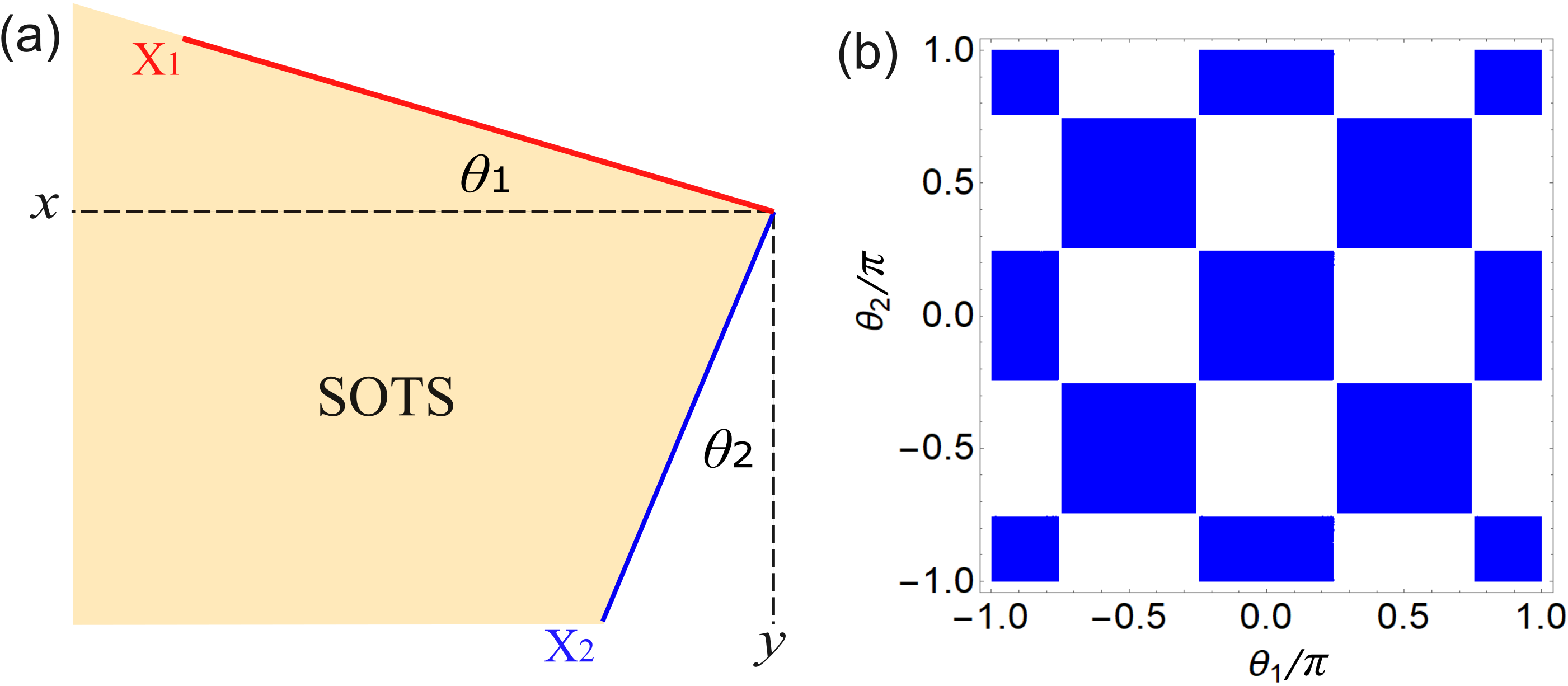
Fig. 4: (a) schematic of two edges with a common corner. (b) The phase diagram for the presence (blue region) and absence (white region) as functions of the two edge directions, $\theta_{1}$ and $\theta_{2}$ (with respect to the $x$ and $y$ axies, respectively).

To form corner states, we need another edge. Let us consider the other edge in $x_{2}$ direction and the SOTS in the $x_{1}<0$ half plane. Along the lines of that we did for the $x_{1}$ edge, we can find analytically the electron and hole edge bands as

$$E_{e,\uparrow}(q_{2}) = -E_{h,\downarrow}(q_{2})=\text{sgn}(mv)q_{2}-\mu,$$ (49)

and their wavefunctions as

$$\Psi_{e,\uparrow,q_{2}}({\bf x}) = \mathcal{N}e^{iq_{2}x_{2}}(e^{\lambda_{1}x_{1}}-e^{\lambda_{1}x_{1}})(\text{sgn}(mv),e^{i\theta})^{T},$$

$$\Psi_{h,\downarrow,q_{2}}({\bf x}) = \Psi_{e,\uparrow,q_{2}}({\bf x}),$$ (50)

where $\lambda_{1(2)}$ and $\mathcal{N}$ are given by Eqs. (39) and (40), respectively. The pairing interaction between the electron and hole bands is found as

$$\Delta_{\text{edge}}^{X_{2}} = -e^{-i\theta}[\Delta_{0}+\Delta_{2}\cos 2\theta(m_{0}/m-2q_{2}^{2})].$$ (51)

At the crossing point $q_{2}=q_{c}=\text{sgn}(mv)\mu/v$ and in the spin basis for $\theta=0$, the pairing gap is given by

$$\widetilde{\Delta}_{\text{gap}}^{X_{2}} = -[\Delta_{0}+\Delta_{2}\cos 2\theta(m_{0}/m-2\mu^{2}/v^{2})].$$ (52)

When $\theta=-\pi/2$ and $0$, we recover again the results for the edges in $y$ and $x$ direction, respectively.

Denote the angle between $x_{1}$ and $x$ direction by $\theta_{1}$, and the angle between $x_{2}$ and $y$ direction by $\theta_{2}$. The pairing gap of the edge states in $x_{1}$ and $x_{2}$ directions are

$$\widetilde{\Delta}_{\text{gap}}^{X_{1}}(\theta_{1})= - [\Delta_{0}-\Delta_{2}\cos 2\theta_{1}(m_{0}/m-2\mu^{2}/v^{2})],$$

$$\widetilde{\Delta}_{\text{gap}}^{X_{2}}(\theta_{2})= - [\Delta_{0}+\Delta_{2}\cos 2\theta_{2}(m_{0}/m-2\mu^{2}/v^{2})].$$ (53)

Note that the spin basis is the same for all edge states (i.e., the spin basis in the particular $x$-$y$ coordinates). The existence of corner states yields that $\widetilde{\Delta}_{\text{gap}}^{X_{1}}(\theta_{1})$ and $\widetilde{\Delta}_{\text{gap}}^{X_{2}}(\theta_{2})$ have different signs,

$$[\Delta_{0}-\Delta_{2}\cos 2\theta_{1}(m_{0}/m-2\mu^{2}/v^{2})]$$

$$\times[\Delta_{0}+\Delta_{2}\cos 2\theta_{2}(m_{0}/m-2\mu^{2}/v^{2})] <0.$$ (54)

For $\Delta_{0}=0$ and considering, in general, $m_{0}/m-2\mu^{2}/v^{2}\neq 0$, Eq. (54) simplifies to

$$\cos 2\theta_{1}\cos 2\theta_{2} > 0.$$ (55)

The phase diagram for corner states is displayed in Fig. 4. One can see that the corner states exist in a wide range of the angles $\theta_{1}$ and $\theta_{2}$ (see the blue areas). This indicates that the corner states, in general, do not require a crystalline symmetry.

Appendix B Calculations of Josephson current

There are different tight-binding lattice models having the low-energy minimal Hamiltonian we consider. In the customary regularization, we can obtain a tight-binding model by replacing $k_{x(y)}\rightarrow\sin k_{x(y)}$ and $k_{x(y)}^{2}\rightarrow 2[1-\cos k_{x(y)}]$. For convenience, the lattice constant is set to unity. Then, Fourier transforming into lattice space, the BdG Hamiltonian is given by

$$\mathcal{H}= \dfrac{1}{2} \sum_{l,l^{\prime}}\sum_{j,j^{\prime}}C_{l,j}^{\dagger}\{(M_{0}\tau_{z}\sigma_{z}-\mu)\delta_{l,l^{\prime}}\delta_{j,j^{\prime}}+\tau_{z}\sigma_{z}$$ (56)

$$\times [m_{x}\delta_{j,j^{\prime}}(\delta_{l,l^{\prime}-1}+\delta_{l,l^{\prime}+1})+m_{y}\delta_{l,l^{\prime}}\left(\delta_{j,j^{\prime}-1}+\delta_{j,j^{\prime}+1}\right)]$$

$$+ i\delta_{j,j^{\prime}}(\delta_{l,l^{\prime}-1}-\delta_{l,l^{\prime}+1})v_{x}\sigma_{x}s_{z}/2+i\delta_{l,l^{\prime}}(\delta_{j,j^{\prime}-1}$$

$$- \delta_{j,j^{\prime}+1})v_{y}\tau_{z}\sigma_{y}/2+\hat{d}_{0}\delta_{l,l^{\prime}}\delta_{j,j^{\prime}}+\hat{d}_{2}\delta_{j,j^{\prime}}(\delta_{l,l^{\prime}-1}$$

$$+ \delta_{l,l^{\prime}+1})-\hat{d}_{2}\delta_{l,l^{\prime}}(\delta_{j,j^{\prime}-1}+\delta_{j,j^{\prime}+1})\}C_{l^{\prime},j^{\prime}}$$

with

$$\hat{d}_{t} = \begin{pmatrix}0&-i\Delta_{t}s_{y}\\ i\Delta_{t}^{*}s_{y}&0\end{pmatrix},\ t\in\{0,2\},$$ (57)

where the spinor operators are $C_{l,j}^{\dagger}=(c_{a,\uparrow;l,j}^{\dagger},c_{b,\uparrow;l,j}^{\dagger},$ $c_{a,\downarrow;l,j}^{\dagger},c_{b,\downarrow;l,j}^{\dagger},c_{a,\uparrow;l,j},c_{b,\uparrow;l,j},c_{a,\downarrow;l,j},c_{b,\downarrow;l,j})$; $M_{0}=m_{0}-2m_{x}-2m_{y}$; $\{l,l^{\prime}\}$ and $\{j,j^{\prime}\}$ denote the lattice sites in $x$ and $y$ directions, respectively. The identity matrices for spin, Nambu and orbital spaces are omitted for ease of notation.

For an SNS junction, the BdG Hamiltonian can be written as

$$\mathcal{H}= \dfrac{1}{2} \sum_{l,l^{\prime}=-\infty}^{\infty}\sum_{j,j^{\prime}=1}^{W}C_{l,j}^{\dagger}\{(M_{0}\tau_{z}\sigma_{z}-\mu_{l})\delta_{l,l^{\prime}}\delta_{j,j^{\prime}}+\tau_{z}\sigma_{z}$$ (58)

$$\times [m_{x}\delta_{j,j^{\prime}}(\delta_{l,l^{\prime}-1}+\delta_{l,l^{\prime}+1})+m_{y}\delta_{l,l^{\prime}}\left(\delta_{j,j^{\prime}-1}+\delta_{j,j^{\prime}+1}\right)]$$

$$+ i\delta_{j,j^{\prime}}(\delta_{l,l^{\prime}-1}-\delta_{l,l^{\prime}+1})v_{x}\sigma_{x}s_{z}/2+i\delta_{l,l^{\prime}}(\delta_{j,j^{\prime}-1}$$

$$- \delta_{j,j^{\prime}+1})v_{y}\tau_{z}\sigma_{y}/2+[\hat{d}_{0,l}\delta_{l,l^{\prime}}\delta_{j,j^{\prime}}+\hat{d}_{2,l}\delta_{j,j^{\prime}}(\delta_{l,l^{\prime}-1}$$

$$+ \delta_{l,l^{\prime}+1})-\hat{d}_{2,l}\delta_{l,l^{\prime}}(\delta_{j,j^{\prime}-1}+\delta_{j,j^{\prime}+1})]$$

$$\times \left[\Theta(1/2-l^{\prime})+\Theta(l^{\prime}+1/2-L)\right]\}C_{l^{\prime},j^{\prime}},$$

where

$$\hat{d}_{t,l} = \begin{pmatrix}0&-i\Delta_{t,l}s_{y}\\ i\Delta_{t,l}^{*}s_{y}&0\end{pmatrix},\ t\in\{0,2\},$$ (59)

and $\Theta(x)$ is the Heaviside step function; $L$ and $W$ (in units of the lattice constant $a$) are the length and width of the junction, respectively. The chemical and pairing potentials are modeled as

$$\mu_{l} =\begin{cases}\mu_{L},&l\leqslant 0\\ \mu_{N},&1\leqslant l\leqslant L,\\ \mu_{R},&l\geqslant L+1\end{cases}\ \Delta_{t,l}=\begin{cases}\Delta_{t},&l\leqslant 0\\ 0,&1\leqslant l\leqslant L.\\ \Delta_{t}e^{i\phi},&l\geqslant L+1\end{cases}$$ (60)

The dc Josephson current can be calculated as (Furusaki, 1994; Martín-Rodero et al., 1994; Asano, 2001)

$$J_{s} =\dfrac{ie}{\hbar}\Big{\langle}\Big{[}\sum_{j}c_{\sigma,s,l,j}^{\dagger}c_{\sigma,s,l,j}^{\dagger},\mathcal{H}\Big{]}\Big{\rangle}$$ (61)

$$=\dfrac{ieT}{2\hbar}\sum_{\omega_{\nu}}\text{Tr}\{\check{\tau}_{3}[\check{H}_{t}\check{\mathcal{G}}(l,l+1,i\omega_{\nu})-\check{H}_{t}^{\dagger}\check{\mathcal{G}}(l+1,i\omega_{\nu})]\},$$

where the over-script $\check{...}$ indicates $8W\text{\text{$\times$}}8W$ matrices expanded in Nambu, spin, orbital, and lattice ($j=1,...,W$) spaces,

$$\check{H}_{t} = (m_{x}\tau_{z}\sigma_{z}-iv_{x}\sigma_{x}s_{z}/2)\text{$\mathbb{I}_{W\times W},$}$$

$$\check{\tau}_{3} = \tau_{3}\text{$\mathbb{I}_{W\times W}.$}$$ (62)

$\check{\mathcal{G}}(l,l^{\prime},i\omega_{\nu})$ is the Matsubara Green’s function, $\omega_{\nu}=(2\nu+1)\pi k_{B}T$ with $\nu=0,\pm 1,...$, is the Matsubara frequency and $T$ is the temperature. $\mathbb{I}_{W\times W}$ denotes the $W\text{\text{$\times$}}W$ identity matrix. We find $\check{\mathcal{G}}(l,l^{\prime},i\omega_{\nu})$ numerically by the recursive Green’s function technique (Lee et al., 1981). The trace is taken over Nambu, spin, orbital, and lattice degrees of freedom. The supercurrent $J_{s}$ is independent of $l$ (Asano, 2001). Thus, it is convenient to calculate $J_{s}$ at $l=L$.

By performing the analytical continuation $i\omega_{\nu}\rightarrow E+i\Gamma$ with a positive infinitesimal $\Gamma$, we obtain the retarded Green’s function $\check{G}^{R}(l,l,E+i\Gamma)$. The density of states is then calculated as

$$\rho(E) = -\dfrac{1}{\pi}\text{Im}[\text{Tr}\check{G}^{R}(l,l,E+i\Gamma)],$$ (63)

where $1\leqslant l\leqslant L$. The energy of Andreev bound states (ABSs) can be found as the peaks of $\rho(E)$. Note that $\rho(E)$ is the same for $l\in\{1,...,L\}$. A small but finite bandwidth $\Gamma$ is employed for the calculation of $\rho(E)$. In this work, we use $\Gamma=10^{-5}m_{0}$ throughout.

To show the $L$-dependence in the supercurrent $J_{s}(\phi)$, we plot in Fig. 5 the current-phase relation for different values of $L$, and $J_{c}$ and $J_{c}L$ as functions of $L$ in the insets (I) and (II), respectively. We can observe that $J_{s}(\phi)$ decays monotonically as we increase $L$. For long junctions $L\gg\text{max}\{v_{x}/|\Delta_{L}|,v_{x}/|\Delta_{R}|\}$, $J_{c}L$ saturates to a constant. This indicates that $J_{c}$ scales as $\sim 1/L$. Moreover, $J_{s}(\phi)$ is insensitive to the width $W$ as long as $W\gg\xi_{\text{edge}}$.

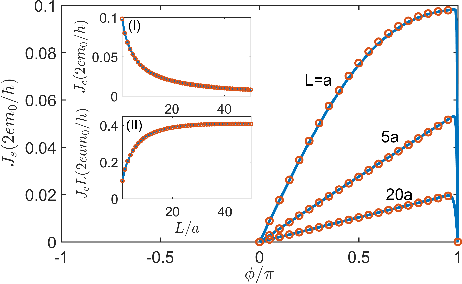
Fig. 5: Current-phase relations $J_{s}(\phi)$ for different lengths $L$ and widths $W$. Here, $L=a,$ 5a, and $20a$ as indicated in the figure. The blue solid curves are for $W=19a$, and the orange circled dots are for $W=9a$. The insets (I) and (II) show the critical current $J_{c}$ and $J_{c}L$ as functions of $L$, respectively. They imply that $J_{c}\sim 1/L$ for long junctions. To quickly converge to the long junction regime, we choose the parameters: $v_{x}=v_{y}=2$, $m_{x}=m_{y}=1$, $\mu_{N}=\mu_{L}=\mu_{R}=0$, $\Delta_{0}=0$ and $\Delta_{2}=0.2$. The units for energy and length(wavenumber) are $m_{0}$ and $a$($a^{-1}$), respectively.

Appendix C Supercurrent from the edge BdG model

In this section, we look at the edge BdG Hamiltonian (33) and derive analytically the ABSs and Majorana bound states (MBSs). Without loss of generality, we assume $m_{y}v_{y}>0$. Then, one edge of the Josephson junction, say the upper one, is described by

$$h_{\text{edge}}^{x} = v_{x}k_{x}\tau_{z}s_{z}-\mu(x)\tau_{z}$$ (64)

$$+\begin{pmatrix}0&0&\Delta(x)&0\\ 0&0&0&-\Delta(x)\\ \Delta^{*}(x)&0&0&0\\ 0&-\Delta^{*}(x)&0&0\end{pmatrix}.$$

where the spatially dependent chemical and pairing potentials are

$$\mu(x) = \mu_{N}\Theta(L/2-|x|)+\mu_{L}\Theta(-x-L/2)$$

$$+\mu_{R}\Theta(x-L/2),$$

$$\Delta(x) = \Delta_{L}\Theta(-x-L/2)+\Delta_{R}e^{i\phi}\Theta(x-L/2).$$ (65)

In the N region, the basis functions can be written as

$$\varphi_{e,+}(x) =(1,0,0,0)^{T}e^{ik_{e}x},$$

$$\varphi_{e,-}(x) =(0,1,0,0)^{T}e^{-ik_{e}x},$$

$$\varphi_{e,+}(x) =(0,0,1,0)^{T}e^{ik_{h}x},$$

$$\varphi_{e,-}(x) =(0,0,0,1)^{T}e^{-ik_{h}x},$$ (66)

where $k_{e(h)}=(\mu_{N}\pm E)/v_{x}.$ Thus, the wavefunction in the N region is expanded as

$$\Psi_{\text{N}}(x) = \sum_{\eta=\pm}\left[A_{e,\eta}\varphi_{e,\eta}(x)+A_{h,\eta}\varphi_{h,\eta}(x)\right],\ |x|<L/2.$$ (67)

In the S leads, the basis functions are

$$\varphi_{qe,+}^{s}(x) = (E+\Omega_{s},0,\Delta_{s}e^{-i\phi_{s}},0)^{T}e^{ik_{eq}^{s}x},$$

$$\varphi_{qh,-}^{s}(x) = (\Delta_{s}e^{i\phi_{s}},0,E+\Omega_{s},0)^{T}e^{ik_{hq}^{s}x},$$

$$\varphi_{qe,-}^{s}(x) = (0,-E-\Omega_{s},0,\Delta_{s}e^{-i\phi_{s}})^{T}e^{-ik_{eq}^{s}x},$$

$$\varphi_{qh,+}^{s}(x) = (0,\Delta_{s}e^{i\phi_{s}},0,-E-\Omega_{s})^{T}e^{-ik_{hq}^{s}x},$$ (68)

where $k_{qe(qh)}^{s}=\mu_{s}\pm\Omega_{s}$ and

$$\Omega_{s} = \begin{cases}\text{sgn}(E)\sqrt{E^{2}-\Delta_{s}^{2}},&E\geqslant\Delta_{s}\\ i\sqrt{\Delta_{s}^{2}-E^{2}},&E<\Delta_{s}\end{cases}$$

with $s\in\{L,R\}$ distinguishing the left and right S leads. $\phi_{L}=0$ and $\phi_{R}=\phi$. We are most interested in the ABSs whose energies satisfy $|E|<\Delta_{s}$. Thus, the wavefunction in the S leads is given by

$$\Psi_{\text{S}}(x) = \begin{cases}B_{eL}\varphi_{e,-}^{L}(x)+B_{hL}\varphi_{qh,-}^{L}(x),&x<-L/2\\ B_{eR}\varphi_{qe,+}^{R}(x)+B_{hR}\varphi_{qh,+}^{R}(x),&x>L/2\end{cases}$$ (69)

The energies $E$ of ABSs and the coefficients $A_{e(h),\pm}$, $B_{e(h)L}$ and $B_{e(h)R}$ are found from the continuity of the wavefunction, i.e.,

$$\Psi_{\text{N}}(-L/2) = \Psi_{\text{S}}(-L/2),\ \Psi_{\text{N}}(L/2)=\Psi_{\text{S}}(L/2).$$ (70)

A nontrivial solution of these equations yields

$$0= [ e^{i(\phi-2EL/v_{x})}\Delta_{L}\Delta_{R}-(E+\Omega_{L})(E+\Omega_{R})]$$ (71)

$$\times [e^{i(\phi+2EL/v_{x})}\Delta_{L}\Delta_{R}-(E+\Omega_{L})(E+\Omega_{R})].$$

This can be recast to the transcendental equations

$$E = \pm\dfrac{\Delta_{L}\Delta_{R}\sin(\phi\pm 2EL/v_{x})}{\sqrt{\Delta_{L}^{2}+\Delta_{R}^{2}-2\Delta_{L}\Delta_{R}\cos(\phi\pm 2EL/v_{x}})}$$ (72)

with $\phi$ satisfying

$$[\cos\left(\phi\pm 2EL/v_{x}\right)-\Delta_{L}/\Delta_{R}]$$

$$\times[\cos\left(\phi\pm 2EL/v_{x}\right)-\Delta_{R}/\Delta_{L}] = 0.$$ (73)

The solutions of $E$ can be found self-consistently from Eq. (72). With the obtained $E$, the coefficients are also obtained. Several salient features of ABSs are obvious: (i) ABSs appear in pairs with opposite energies; (ii) the ABS spectrum is independent $\mu_{N}$; (iii) more ABS branches appear for a longer $L$.

In the short junction limit $L=0$, the ABS spectrum can be found analytically as

$$E_{\pm}(\phi) = \pm\dfrac{\Delta_{L}\Delta_{R}\sin\phi}{\sqrt{\Delta_{L}^{2}+\Delta_{R}^{2}-2\Delta_{L}\Delta_{R}\cos\phi}}.$$ (74)

Correspondingly, equation (73) defines the parameter range for the existence of ABSs

$$\left(\cos\phi-\Delta_{L}/\Delta_{R}\right)\left(\cos\phi-\Delta_{R}/\Delta_{L}\right) = 0.$$ (75)

Note that for the 0-junction, $\Delta_{L}\Delta_{R}>0$, while for the $\pi$-junction, $\Delta_{L}\Delta_{R}<0$. From Eqs. (74) and (75), it is easy to see that the zero-energy modes are at $\phi=\pm\pi$ in the 0-junction, while they switched to be at $\phi=0$ in the $\pi$-junction. Note that this result holds also in longer junctions. In both junctions, the wavefunctions of two zero-energy modes can be written in a compact form

$$\Psi_{+}(x) = \eta(x)(-i,0,\text{sgn}(\Delta_{L}),0)^{T},$$

$$\Psi_{-}(x) = \eta^{*}(x)(0,\text{sgn}(\Delta_{L}),0,i)^{T},$$ (76)

where

$$\eta(x) = e^{(i\mu_{L}+|\Delta_{L}|)x\Theta(-x)+(i\mu_{R}-|\Delta_{R}|)x\Theta(x)}.$$ (77)

Restoring the basis $(\Psi_{e,\uparrow},\Psi_{e,\downarrow},\Psi_{h,\downarrow},\Psi_{h,\uparrow}),$ we can write

$$\Psi_{+}(x) = -i\eta(x)\Psi_{e,\uparrow}+\text{sgn}(\Delta_{L})\eta(x)\Psi_{h,\downarrow},$$

$$\Psi_{-}(x) = \text{sgn}(\Delta_{L})\eta^{*}(x)\Psi_{e,\downarrow}+i\eta^{*}(x)\Psi_{h,\uparrow},$$ (78)

Recall Eqs. (29), $\Psi_{h,\uparrow/\downarrow}=\Psi_{e,\uparrow/\downarrow}^{*}.$ Hence, the two zero-energy modes obey

$$\Psi_{+}(x) = \Psi_{-}^{*}(x).$$ (79)

This indicates that they are related by particle-hole symmetry. We can recombine them and obtain

$$\gamma_{+}(x) = \Psi_{+}(x)+\Psi_{-}(x),$$

$$\gamma_{-}(x) = i[\Psi_{+}(x)-\Psi_{-}(x)].$$ (80)

The new zero-energy modes have self-adjoint wavefunctions

$$\gamma_{\pm}(x) = \gamma_{\pm}^{*}(x),$$ (81)

and behave like MBSs. Under time-reversal operation $\mathcal{T}$,

$$\mathcal{T}\Psi_{e,\downarrow} = \Psi_{e,\uparrow}^{*},\ \mathcal{T}\Psi_{e,\uparrow}=-\Psi_{e,\downarrow}^{*},$$

$$\mathcal{T}\Psi_{h,\downarrow} = \Psi_{h\uparrow}^{*},\ \mathcal{T}\Psi_{h,\uparrow}=-\Psi_{h,\downarrow}^{*}.$$ (82)

This shows that the two MBSs are connected by time-reversal symmetry,

$$\mathcal{T}\gamma_{+}(x) = \gamma_{-}(x).$$ (83)

Hence, they are Kramers partners.

Appendix D Symmetries and quadrupole moment

In this section, we analyze the symmetries and calculate the quadrupole moment of the SOTS.

D.1 Symmetries

The BdG Hamiltonian Eq. (1) in the main text

$$H_{\text{BdG}}({\bf k}) = m({\bf k})\tau_{z}\sigma_{z}+v_{x}k_{x}s_{z}\sigma_{x}+v_{y}k_{y}\tau_{z}\sigma_{y}$$ (84)

$$+\Delta({\bf k})\tau_{y}s_{y}-\mu\tau_{z}$$

satisfies the following symmetries:
$\bullet$ time-reversal symmetry, $\mathcal{T}=is_{y}\mathcal{K}$ with $\mathcal{K}$ the complex conjugation:

$$\mathcal{T}H_{\text{BdG}}({\bf k})\mathcal{T}^{-1}=H_{\text{BdG}}({\bf-k});$$ (85)

$\bullet$ particle-hole symmetry, $\Xi=\tau_{x}\mathcal{K}$:

$$\Xi H_{\text{BdG}}({\bf k})\Xi^{-1}=-H_{\text{BdG}}({\bf-k});$$ (86)

$\bullet$ inversion symmetry, $\mathcal{P}=\sigma_{z}$:

$$\mathcal{P}H_{\text{BdG}}({\bf k})\mathcal{P}^{-1} =H_{\text{BdG}}({\bf-k});$$ (87)

$\bullet$ if $\mu=0$, combined reflection symmetries, $\mathcal{M}_{x}=\tau_{x}s_{x}\sigma_{x}$ and $\mathcal{\mathcal{M}}_{y}=\tau_{x}s_{x}\sigma_{y}$:

$$\mathcal{M}_{x}H_{\text{BdG}}({\bf k})\mathcal{\mathcal{M}}_{x}^{-1} =H_{\text{BdG}}(-k_{x},k_{y}),$$

$$\mathcal{\mathcal{M}}_{y}H_{\text{BdG}}({\bf k})\mathcal{\mathcal{M}}_{y}^{-1} =H_{\text{BdG}}(k_{x},-k_{y});$$ (88)

$\bullet$ if $m_{x}=m_{y}$, $v_{x}=v_{y}=v$ and $\Delta_{0}=0$, combined four-fold rotation symmetry, $\mathcal{C}_{4}=\tau_{z}e^{i\pi\sigma_{z}/4}$:

$$\mathcal{C}_{4}H_{\text{BdG}}({\bf k})\mathcal{C}_{4}^{-1}=H_{\text{BdG}}(k_{y},-k_{x}).$$ (89)

D.2 Quadrupole moment

To find the quadrupole moment by the Wilson-loop approach of Benalcazar et al. (2017a, b), we need to consider a periodic lattice model. As the previous numerical calculations, we consider the lattice model by replacing $k_{x(y)}\rightarrow\sin k_{x(y)}$ and $k_{x(y)}^{2}\rightarrow 2[1-\cos k_{x(y)}]$ in Eq. (84)

The projected position operator $P^{\text{occ}}\hat{x}P^{\text{occ}}$ into the occupied bands can define a Wilson line. In $x$ direction, the Wilson line operator is given by

$$\mathcal{W}_{k_{f}\leftarrow k_{i}}=F_{k_{f}-\delta_{k}}F_{k_{f}-2\delta_{k}}\cdots F_{k_{i}+\delta_{k}}F_{k_{i}},$$ (90)

where $[F_{k}]^{nn^{\prime}}=\langle u_{k+\delta_{k_{x}}}^{n}|u_{k}^{n^{\prime}}\rangle$, $\delta_{k_{x}}=2\pi/N_{x}$ and $|u_{k}^{n}\rangle$ are the eigenstates of the lattice Hamiltonian. $N_{x}$ is the number of lattice sites in $x$ direction. For the limit $N_{x}\rightarrow\infty$, $[F_{k}]^{nn^{\prime}}\approx e^{-iA_{nn^{\prime}}\delta_{k}}$ with $A_{nn^{\prime}}=i\langle u_{k}^{n}|\partial_{k_{x}}u_{k}^{n^{\prime}}\rangle$ the non-Abelian gauge field.

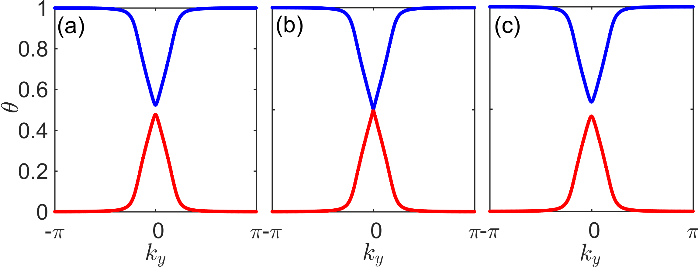
Fig. 6: Wannier bands $\theta_{x}^{+}$ (blue) and $\theta_{x}^{-}$ (red) of occupied states in $x$ direction for $\Delta_{0}=0$ (a), $0.04m_{0}$ (b) and $0.1m_{0}$ (c). The Wannier bands do not touch at any point over $k_{y}\in(-\pi,\pi]$ except for the special case with $\Delta_{0}=2\Delta_{2}m_{0}/m$. Other parameters are $\mu=0$, $m=2.5$, $m_{0}=1$, $A=1$ and $\Delta_{2}=0.2$ (we choose a larger $\Delta_{2}$ in order to make the Wannier gap more visible).

A Wilson loop $\mathcal{W}_{k_{x}+2\pi\leftarrow k_{x}}$ is defined as a Wilson line that goes across the entire Brillouin zone. It is unitary and its eigenvalues take the form

$$E_{j,R}=e^{i\delta_{k}(\theta_{x}^{j}+R)},$$ (91)

where $R\in\{0,1,...,N-1\}$. The phases $\theta_{x}^{j}$ of the eigenvalues are called the Wannier centers. They correspond to the position of the electrons relative to the center of the unit cell (Yu et al., 2010). The Wilson loop can be connected to the Wannier Hamiltonian $H_{\mathcal{W}}(k)$ of the edge, $\mathcal{W}_{x,k}\equiv e^{iH_{\mathcal{W}}(k)}.$ It can be adiabatically related to the physical Hamiltonian of the $x$ edge (Fidkowski et al., 2010). Correspondingly, $\theta_{x}^{j}(k_{y})$ with $j\in\{1,...,N_{\text{occ}}\}$ are refereed to the Wannier spectrum (or bands). It depends on the $k_{y}$ coordinate. Given the normalized Wilson-loop eigenstate, the eigenstates of $\mathcal{W}_{k_{x}+2\pi\leftarrow k_{x}}$ are written as

$$|w_{k}^{j}\rangle =\sum_{n=1}^{N_{\text{occ}}}[v_{k}^{j}]^{n}\gamma_{n,k}^{\dagger}|0\rangle,$$ (92)

where $[v_{k}^{j}]^{n}$ is the $n$th component of the $j$th Wilson-loop eigenstate $|v_{k}^{j}\rangle$. Note that while the Wilson-loop eigenvalues $\theta_{x}^{j}$ do not depend on the base point $k_{x}$, their eigenstates $|v^{j}\rangle$ do. The electronic contribution to the dipole moment, called polarization, is proportional to

$$p_{x}(k_{y})=\sum_{j}\theta_{x}^{j}(k_{y})\ \text{mod\ }1.$$ (93)

Consider the SOTS with $\mu=0$ and vary $\Delta_{0}$. There are $N_{\text{occ}}=2$ Wannier bands $\theta_{x}^{\pm}(k_{y})$ corresponding to the two occupied bands, as shown in Fig. 6. These two Wannier bands, in general, do not touch at any point over $k_{y}$ except for $\Delta_{0}=2\Delta_{2}m_{0}/m$. They obey $\theta_{x}^{+}(k_{y})+\theta_{x}^{-}(k_{y})=0$ mod 1. Thus, the total polarization is always zero. We can define the two Wannier bands as $\theta_{x}^{+}\in[0,1/2)$ and $\theta_{x}^{-}\in(1/2,1]$.

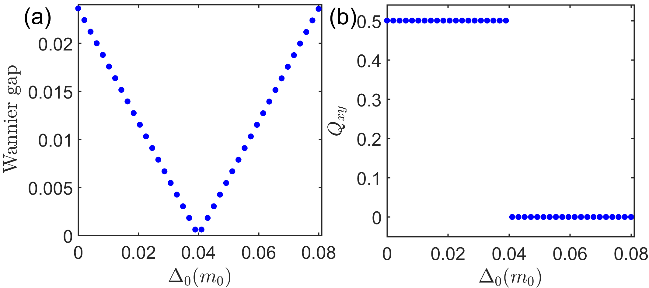
Fig. 7: (a) Wannier gap, $\text{min}(|\theta_{x}^{+}-\theta_{x}^{-}|)$, as a function of $\Delta_{0}$; (b) quadrupole moment as a function of $\Delta_{0}$. Other parameters are the same as those in Fig. 6.

Following a similar approach as that for the lattice model, we can define a nested Wilson loop $\mathcal{\widetilde{W}}_{k_{y}+2\pi\leftarrow k_{y}}$ for the Wannier bands with the Wannier functions given by Eq. (92) and calculate the associated polarization $p_{y}^{\theta_{x}^{\pm}}$. Under reflections $\mathcal{M}_{x}$, $\mathcal{M}_{y}$, and inversion $\mathcal{I}$, the Wannier sector polarization obey

$$p_{y}^{\theta_{x}^{+}} \overset{\mathcal{I}}{=} -p_{y}^{\theta_{x}^{-}},\ p_{y}^{\theta_{x}^{+}}\overset{\mathcal{M}_{x}}{=}p_{y}^{\theta_{x}^{-}},\ p_{y}^{\theta_{x}^{\pm}}\overset{\mathcal{M}_{y}}{=}-p_{y}^{\theta_{x}^{\pm}}$$ (94)

mod 1. Thus, $p_{y}^{\theta_{x}^{\pm}}$ must quantize (at 0 or $1/2$) in the presence of the symmetries $\mathcal{M}_{x}$, $\mathcal{M}_{y}$ and $\mathcal{I}$. The relations and result for the other Wannier polarization $p_{x}^{\theta_{y}^{\pm}}$ are the same as above but with exchanging $x\leftrightarrow y$. In reflection symmetric insulators, the Wannier polarization can be alternatively computed from the eigenvalues of symmetry operators at the reflection-invariant momenta (Benalcazar et al., 2017b). The existence of corner states can be associated with the quantized polarization $p_{y}^{\theta_{x}^{\pm}},p_{x}^{\theta_{y}^{\pm}}=1/2$.

The quadrupole moment $Q_{xy}$ can be written as

$$Q_{xy}=2p_{y}^{\theta_{x}^{\pm}}p_{x}^{\theta_{y}^{\pm}}.$$ (95)

The SOTS at $\mu=0$ preserves $\mathcal{M}_{x}$ and $\mathcal{M}_{y}$ symmetries. Thus, $Q_{xy}$ is always quantized and can be identified as the topological invariant for the SOTS. When increasing $\Delta_{0}$, the quadrupole moment changes from 1/2 to 0 at $\Delta_{0}=2\Delta_{2}m_{0}/m$ where the Wannier gap closes, as shown in Fig. 7. However, when $\mu\neq 0$, both $\mathcal{M}_{x}$ and $\mathcal{M}_{y}$ symmetries are broken. Then, $Q_{xy}$ is no longer quantized. Nevertheless, since we can smoothly vary $\mu$ to the particular limit (with $\mathcal{M}_{x}$ and $\mathcal{M}_{y}$ symmetries) without closing either the bulk or edge gap, the general SOTS phase is topologically equivalent to the SOTSs that preserve these reflection symmetries.

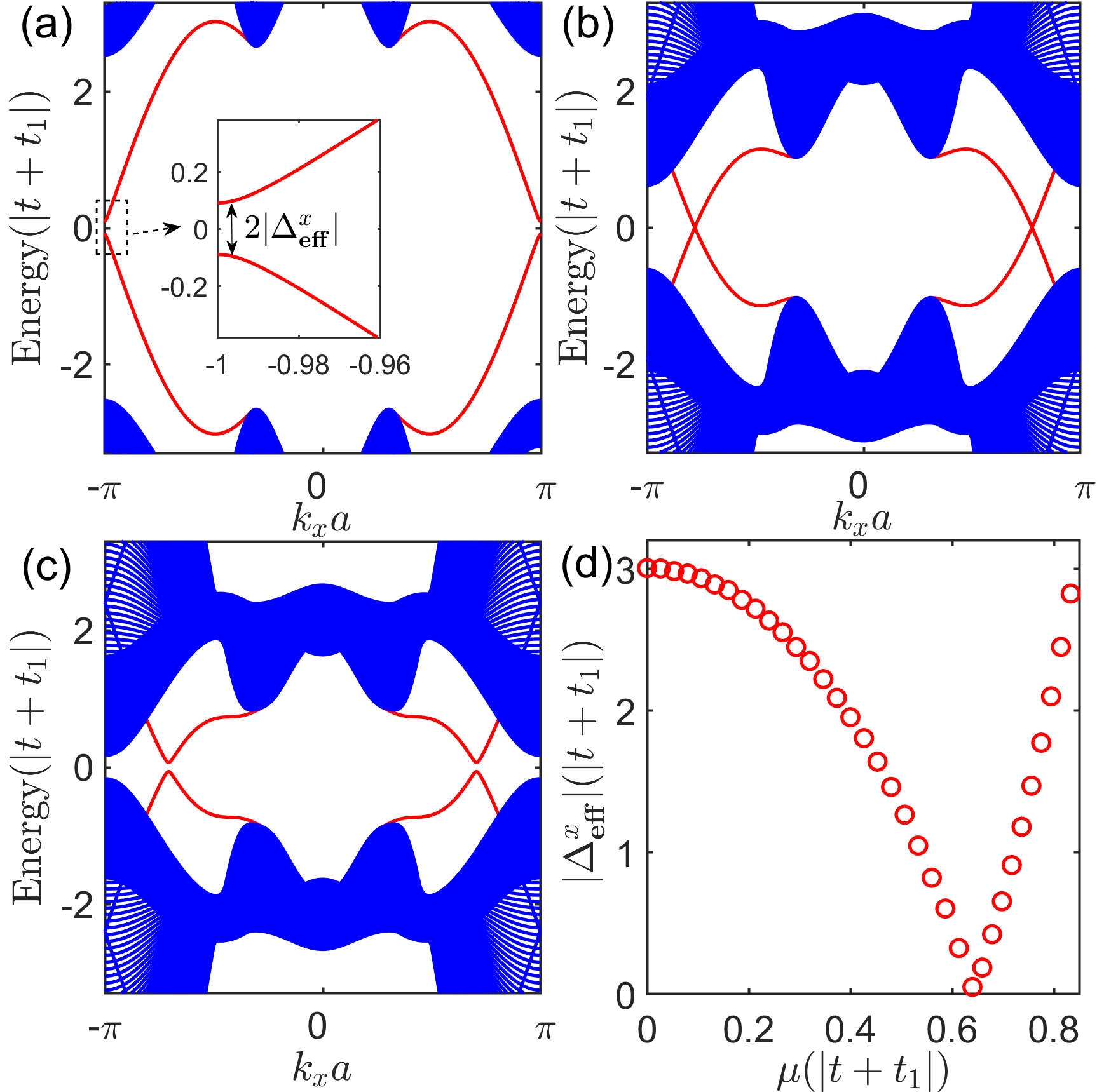
Fig. 8: (a-c) Energy spectra of the lattice model (96) in a ribbon geometry along $x$ direction for the chemical potential $\mu=0$, $0.64|t+t_{1}|$ and $0.8|t+t_{1}|$, respectively. The red curves corresponds to the edge bands while the blue ones are the bulk bands. (d) Edge pairing gap $|\Delta_{\text{eff}}^{x}|$ as a function of $\mu$. One can observe a gap closing of $\Delta_{\text{eff}}^{x}$ as increasing $\mu$. Other parameters are $t=2$, $t_{1}=1$, $\lambda=1.5$, $a=1$, $\Delta_{0}=0.12|t+t_{1}|$ and $\Delta_{2}=0.05|t+t_{1}|$. The number of lattice sites in $y$ direction is $L_{y}=200$.

Appendix E Results from another typical lattice model

In this section, we will show that the minimal model can be derived from different lattice models for SOTSs at low energies. For instance, we consider another typical lattice model for SOTSs given by (Wang et al., 2018a)

$$H_{\text{BdG}} = M({\bf k})\tau_{z}\sigma_{z}+2\lambda(\sin k_{x}s_{y}-\sin k_{y}s_{x})\tau_{z}\sigma_{x}$$ (96)

$$-\mu\tau_{z}+\Delta({\bf k})\tau_{x}$$

in the basis $(c_{a,\uparrow},c_{a,\downarrow},c_{b,\uparrow},c_{b,\downarrow},c_{a,\uparrow}^{\dagger},c_{a,\downarrow}^{\dagger},c_{b,\uparrow}^{\dagger},c_{b,\downarrow}^{\dagger})$, where $M({\bf k})=2t(\cos k_{x}-\cos k_{y})+4t_{1}\cos k_{x}\cos k_{y}$ and $\Delta({\bf k})=\Delta_{0}+2\Delta_{2}(\cos k_{x}+\cos k_{y})$ with $|\Delta_{0}|<2|\Delta_{2}|$. The Pauli matrices $\bm{\tau}$, $\bm{\sigma}$ and ${\bf s}$ act on Nambu, orbital and spin spaces, respectively. This lattice model describes a QSHI with $s_{\pm}$-wave pairing potential but with band inversion at the $X=(\pi,0)$ point.

Around the $X$ point, we expand all terms up to quadratic order in momentum ${\bf k}$:

$$M({\bf k}) \rightarrow m({\bf k})=-4(t+t_{1})+(t+2t_{1})|{\bf k}|^{2},$$

$$\sin k_{x} \rightarrow -k_{x},\ \ \sin k_{y}\rightarrow k_{y},$$

$$\Delta({\bf k}) \rightarrow \Delta_{0}+\Delta_{2}(k_{x}^{2}-k_{y}^{2}).$$ (97)

Here, ${\bf k}$ is measured from the $X$ point. Rearranging the basis to $(c_{a,\uparrow},-c_{b,\downarrow},c_{a,\downarrow},c_{b,\uparrow},c_{a,\downarrow}^{\dagger},c_{b,\uparrow}^{\dagger},-c_{a,\uparrow}^{\dagger},c_{b,\downarrow}^{\dagger})$, we then obtain the low-energy effective model as

$$H_{\text{BdG}} \rightarrow \begin{pmatrix}m({\bf k})-\mu&2\lambda k_{-}&0&0&0&0&-\Delta({\bf k})&0\\ 2\lambda k_{+}&-m({\bf k})-\mu&0&0&0&0&0&-\Delta({\bf k})\\ 0&0&m({\bf k})-\mu&-2\lambda k_{+}&\Delta({\bf k})&0&0&0\\ 0&0&-2\lambda k_{-}&-m({\bf k})-\mu&0&\Delta({\bf k})&0&0\\ 0&0&\Delta({\bf k})&0&-m({\bf k})+\mu&2\lambda k_{+}&0&0\\ 0&0&0&\Delta({\bf k})&2\lambda k_{-}&m({\bf k})+\mu&0&0\\ -\Delta({\bf k})&0&0&0&0&0&-m({\bf k})+\mu&-2\lambda k_{-}\\ 0&-\Delta({\bf k})&0&0&0&0&-2\lambda k_{+}&m({\bf k})+\mu\end{pmatrix},$$ (98)

where $k_{\pm}=k_{y}\pm ik_{x}$. It takes the some form of the minimal model (1) in the main text.

Taking a set of parameters that satisfy the large inverted gap condition, the energy spectra of the lattice model (96) of a ribbon geometry in $x$ direction are presented in Fig. 8. At $k_{x}=\pm\pi$, band inversion happens and edge states appear nearby. More importantly, with increasing the chemical potential from zero, we can again observe a gap closing and reopening at the edge states without closing the bulk gap.

References

Langbehn et al. (2017)J. Langbehn, Y. Peng,
L. Trifunovic, F. von Oppen, and P. W. Brouwer, “Reflection-Symmetric Second-Order
Topological Insulators and Superconductors,” Phys. Rev. Lett. 119, 246401 (2017).
Khalaf (2018)E. Khalaf, “Higher-order
topological insulators and superconductors protected by inversion
symmetry,” Phys. Rev. B 97, 205136 (2018).
Liu et al. (2018)T. Liu, J. J. He, and F. Nori, “Majorana corner states in a
two-dimensional magnetic topological insulator on a high-temperature
superconductor,” Phys. Rev. B 98, 245413 (2018).
Geier et al. (2018)M. Geier, L. Trifunovic,
M. Hoskam, and P. W. Brouwer, “Second-order topological insulators and
superconductors with an order-two crystalline symmetry,” Phys.
Rev. B 97, 205135
(2018).
Zhu (2018)X. Zhu, “Tunable Majorana
corner states in a two-dimensional second-order topological superconductor
induced by magnetic fields,” Phys. Rev. B 97, 205134 (2018).
Wang et al. (2018)Y. Wang, M. Lin, and T. L. Hughes, “Weak-pairing higher order topological superconductors,” Phys. Rev. B 98, 165144 (2018).
Hsu et al. (2018)C.-H. Hsu, P. Stano, J. Klinovaja, and D. Loss, “Majorana Kramers Pairs in Higher-Order
Topological Insulators,” Phys. Rev. Lett. 121, 196801 (2018).
Zhang et al. (2019a)R.-X. Zhang, W. S. Cole, and S. Das Sarma, “Helical Hinge Majorana
Modes in Iron-Based Superconductors,” Phys. Rev. Lett. 122, 187001 (2019a).
(11)S. Qin, L. Hu,
C. Le, J. Zeng, F.-C. Zhang, C. Fang, and J. Hu, “Quasi 1D topological nodal vortex line phase in doped superconducting 3D
Dirac Semimetals,” arXiv:1901.04932 .
Bultinck et al. (2019)N. Bultinck, B. A. Bernevig, and M. P. Zaletel, “Three-dimensional superconductors with hybrid higher-order topology,” Phys. Rev. B 99, 125149 (2019).
Peng et al. (2019)Y. Peng and Y. Xu, “Proximity-induced Majorana hinge modes in antiferromagnetic topological insulators,” Phys. Rev. B 99, 195431 (2019).
Kitaev (2001)A. Y. Kitaev, “Unpaired
Majorana fermions in quantum wires,” Phys. Usp. 44, 131 (2001).
Kitaev (2003)A Y. Kitaev, “Fault-tolerant
quantum computation by anyons,” Ann. Phys. 303, 2
(2003).
Nayak et al. (2008)C. Nayak, S. H. Simon,
A. Stern, M. Freedman, and S. Das Sarma, “Non-Abelian anyons and topological quantum
computation,” Rev. Mod. Phys. 80, 1083 (2008).
Alicea (2012)J. Alicea, “New directions
in the pursuit of Majorana fermions in solid state systems,” Rep. Prog. Phys. 75, 076501 (2012).
Leijnse and Flensberg (2012)M. Leijnse and K. Flensberg, “Introduction
to topological superconductivity and Majorana fermions,” Semicond. Sci. Technol. 27, 124003 (2012).
Elliott and Franz (2015)S. R. Elliott and M. Franz, “Colloquium:
Majorana fermions in nuclear, particle, and solid-state physics,” Rev. Mod. Phys. 87, 137 (2015).
Sarma et al. (2015)S. Das Sarma, M. Freedman, and C. Nayak, “Majorana zero modes and topological
quantum computation,” npj Quantum Inf. 1, 15001 (2015).
(23)E. J. König and P. Coleman, “Helical
Majorana modes in iron based Dirac superconductors,” arXiv:1901.03692 .
Volpez et al. (2019)Y. Volpez, D. Loss, and J. Klinovaja, “Second-Order Topological
Superconductivity in -Junction Rashba Layers,” Phys. Rev. Lett. 122, 126402 (2019).
Shapourian et al. (2018)H. Shapourian, Y. Wang, and S. Ryu, “Topological crystalline
superconductivity and second-order topological superconductivity in
nodal-loop materials,” Phys. Rev. B 97, 094508 (2018).
(26)X.-H. Pan, K.-J. Yang,
L. Chen, G. Xu, C.-X. Liu, and X. Liu, “Lattice symmetry assisted second order topological
superconductors and Majorana patterns,” arXiv:1812.10989 .
(27)M. Kheirkhah, Y. Nagai, C. Chen, and F. Marsiglio, “Majorana corner flat bands
in two-dimensional second-order topological superconductors,” arXiv:1904.00990
.
(28)S. A. A. Ghorashi, X. Hu, T. L. Hughes, and E. Rossi, “Second-order Dirac superconductors and magnetic field induced
Majorana hinge modes,” arXiv:1901.07579 .
Linder and Sudbø (2008)J. Linder and A. Sudbø, “Tunneling
conductance in - and -wave superconductor-graphene junctions: Extended
Blonder-Tinkham-Klapwijk formalism,” Phys.
Rev. B 77, 064507
(2008).
Linder et al. (2010)J. Linder, Y. Tanaka,
T. Yokoyama, A. Sudbø, and N. Nagaosa, “Unconventional Superconductivity on a
Topological Insulator,” Phys. Rev. Lett. 104, 067001 (2010).
Black-Schaffer and Balatsky (2013)A. M. Black-Schaffer and A. V. Balatsky, “Proximity-induced unconventional superconductivity in topological
insulators,” Phys. Rev. B 87, 220506(R) (2013).
Zhang et al. (2013)F. Zhang, C. L. Kane, and E. J. Mele, “Time-Reversal-Invariant
Topological Superconductivity and Majorana Kramers Pairs,” Phys. Rev. Lett. 111, 056402 (2013).
Li et al. (2015)Z.-X. Li, C. Chan, and H. Yao, “Realizing majorana zero modes by
proximity effect between topological insulators and -wave high-temperature
superconductors,” Phys. Rev. B 91, 235143 (2015).
Zareapour et al. (2016)P. Zareapour, J. Xu,
S. Yang F. Zhao, A. Jain, Z. Xu, T. S. Liu, G. D. Gu, and K. S. Burch, “Modeling tunneling for the unconventional superconducting proximity
effect,” Supercond. Sci. Tech. 29, 125006 (2016).
Li et al. (2016)W.-J. Li, S.-P. Chao, and T.-K. Lee, “Theoretical study of large
proximity-induced -wave-like pairing from a -wave superconductor,” Phys. Rev. B 93, 035140 (2016).
Wu et al. (2016)X. Wu, S. Qin, Y. Liang, H. Fan, and J. Hu, “Topological characters in
thin
films,” Phys. Rev. B 93, 115129 (2016).
Wang et al. (2015)Z. Wang, P. Zhang,
G. Xu, L. K. Zeng, H. Miao, X. Xu, T. Qian, H. Weng, P. Richard, A. V. Fedorov, H. Ding, X. Dai, and Z. Fang, “Topological nature of the
superconductor,” Phys. Rev. B 92, 115119 (2015).
Zhou et al. (2019)T. Zhou, Y. Gao, and Z. D. Wang, “Detecting competing orders through the
edge states in the heterostructures with high- superconductors,” Phys. Rev. B 99, 104517 (2019).
Zareapour et al. (2012)P. Zareapour, A. Hayat,
S. Y. F. Zhao, M. Kreshchuk, A. Jain, D. C. Kwok, N. Lee, S.-W. Cheong, Z. Xu, A. Yang, et al., “Proximity-induced high-temperature superconductivity in the topological
insulators Bi2Se3 and Bi2Te3,” Nat.
Commun. 3, 1056
(2012).
Wang et al. (2013)E. Wang, H. Ding, A. V. Fedorov, W. Yao, Z. Li, Y.-F. Lv, K. Zhao, L.-G. Zhang,
Z. Xu, J. Schneeloch, et al., “Fully gapped topological surface states
in Bi2Se3 films induced by a d-wave high-temperature
superconductor,” Nat. Phys. 9, 621 (2013).
Zhao et al. (2018)H. Zhao, B. Rachmilowitz,
Z. Ren, R. Han, J. Schneeloch, R. Zhong, G. Gu, Z. Wang, and I. Zeljkovic, “Superconducting proximity effect in a topological insulator using Fe(Te,
Se),” Phys. Rev. B 97, 224504 (2018).
Perconte et al. (2018)D. Perconte, F. A. Cuellar, C. Moreau-Luchaire, M. Piquemal-Banci, R. Galceran, P. R Kidambi, M.-B. Martin,
S. Hofmann, R. Bernard, B. Dlubak, et al., “Tunable Klein-like tunnelling of
high-temperature superconducting pairs into graphene,” Nat. Phys. 14, 25 (2018).
Xu et al. (2014)S.-Y. Xu, C. Liu, A. Richardella, I. Belopolski, N. Alidoust, M. Neupane, G. Bian, N. Samarth, and M. Z. Hasan, “Fermi-level
electronic structure of a topological-insulator/cuprate-superconductor based
heterostructure in the superconducting proximity effect regime,” Phys. Rev. B 90, 085128 (2014).
Yilmaz et al. (2014)T. Yilmaz, I. Pletikosić, A. P. Weber, J. T. Sadowski, G. D. Gu, A. N. Caruso, B. Sinkovic, and T. Valla, “Absence of a Proximity Effect for a Thin-Films of a
Topological Insulator Grown on Top of a
Cuprate Superconductor,” Phys. Rev. Lett. 113, 067003 (2014).
Qian et al. (2014)X. Qian, J. Liu, L. Fu, and J. Li, “Quantum spin hall effect in two-dimensional transition
metal dichalcogenides,” Science 346, 1344 (2014).
Tang et al. (2017)S. Tang, C. Zhang,
D. Wong, Z. Pedramrazi, H.-Z. Tsai, C. Jia, B. Moritz, M. Claassen, H. Ryu, S. Kahn, et al., “Quantum spin Hall state in monolayer 1T’-WTe2,” Nat. Phys. 13, 683 (2017).
Fei et al. (2017)Z. Fei, T. Palomaki,
S. Wu, W. Zhao, X. Cai, B. Sun, P. Nguyen,
J. Finney, X. Xu, and D. H. Cobden, “Edge conduction in monolayer WTe2,” Nat. Phys. 13, 677 (2017).
Wu et al. (2018)S. Wu, V. Fatemi, Q. D. Gibson, K. Watanabe, T. Taniguchi, R. J. Cava, and P. Jarillo-Herrero, “Observation of the quantum spin Hall effect up
to 100 kelvin in a monolayer crystal,” Science 359, 76 (2018).
Chen et al. (2018)P Chen, W. W. Pai,
Y.-H. Chan, W.-L. Sun, C.-Z. Xu, D.-S. Lin, M. Y. Chou, A.-V. Fedorov, and T.-C. Chiang, “Large
quantum-spin-Hall gap in single-layer 1T’-WSe2,” Nat.
Commun. 9, 2003
(2018).
Weng et al. (2015)H. Weng, A. Ranjbar,
Y. Liang, Z. Song, M. Khazaei, S. Yunoki, M. Arai, Y. Kawazoe, Z. Fang, and X. Dai, “Large-gap two-dimensional topological
insulator in oxygen functionalized MXene,” Phys.
Rev. B 92, 075436
(2015).
Si et al. (2016)C. Si, K.-H. Jin,
J. Zhou, Z. Sun, and F. Liu, “Large-Gap Quantum Spin Hall State in MXenes: d-Band
Topological Order in a Triangular Lattice,” Nano Lett. 16, 6584
(2016).
Reis et al. (2017)F. Reis, G. Li, L. Dudy, M. Bauernfeind, S. Glass, W. Hanke, R. Thomale, J. Schäfer, and R. Claessen, “Bismuthene on a SiC substrate: A candidate for a high-temperature
quantum spin Hall material,” Science 357, 287 (2017).
Hsu et al. (2015)C.-H. Hsu, Z.-Q. Huang,
F.-C. Chuang, C.-C. Kuo, Y.-T. Liu, H. Lin, and A. Bansil, “The nontrivial electronic structure of Bi/Sb honeycombs on SiC(0001),” New J. Phys. 17, 025005 (2015).
Wrasse and Schmidt (2014)E. O. Wrasse and T. M. Schmidt, “Prediction of
Two-Dimensional Topological Crystalline Insulator in PbSe Monolayer,” Nano Lett. 14, 5717 (2014).
Liu et al. (2015)J. Liu, X. Qian, and L. Fu, “Crystal Field Effect Induced
Topological Crystalline Insulators In Monolayer IVšCVI Semiconductors,” Nano Lett. 15, 2657 (2015).
Wan et al. (2017)W. Wan, Y. Yao, L. Sun, C.-C. Liu, and F. Zhang, “Topological, valleytronic, and optical properties of
monolayer PbS,” Adv. Mater. 29, 1604788 (2017).
Bernevig et al. (2006)B. A. Bernevig, T. L. Hughes, and S.-C. Zhang, “Quantum Spin
Hall Effect and Topological Phase Transition in HgTe Quantum Wells,” Science 314, 1757 (2006).
Hirschfeld et al. (2011)P. J. Hirschfeld, M. M. Korshunov, and I. I. Mazin, “Gap symmetry and
structure of Fe-based superconductors,” Rep. Prog. Phys. 74, 124508 (2011).
Zhang et al. (2018)P. Zhang, K. Yaji,
T. Hashimoto, Y. Ota, T. Kondo, K. Okazaki, Z. Wang, J. Wen, G. D. Gu,
H. Ding, and S. Shin, “Observation of topological superconductivity on
the surface of an iron-based superconductor,” Science 360, 182
(2018).
Wang et al. (2018b)D. Wang, L. Kong, P. Fan, H. Chen, S. Zhu, W. Liu, L. Cao, Y. Sun, S. Du, J. Schneeloch, R. Zhong, G. Gu, L. Fu, H. Ding, and H.-J. Gao, “Evidence for Majorana bound states in
an iron-based superconductor,” Science 362, 333 (2018b).
Zhang et al. (2019b)P. Zhang, Z. Wang,
X. Wu, K. Yaji, Y. Ishida, Y. Kohama, G. Dai, Y. Sun, C. Bareille,
K. Kuroda, et al., “Multiple
topological states in iron-based superconductors,” Nat.
Phys. 15, 41 (2019b).
Note (5)Hard-wall boundary conditions are applicable because of the quadratic terms in our low-energy model.
Zhang et al. (2016)S.-B. Zhang, H.-Z. Lu, and S.-Q. Shen, “Linear magnetoconductivity
in an intrinsic topological Weyl semimetal,” New J. Phys. 18, 053039 (2016).
Note (1)For convenience, we assume the pairing potential independent of chemical potential . This should be
justified since is induced via the proximity
effect.
(66)See the Supplemental Material for the
details .
Jackiw and Rebbi (1976) R. Jackiw and C. Rebbi, “Solitons with fermion number 1/2,” Phys.
Rev. D 13, 3398
(1976).
Benalcazar et al. (2017a)W. A. Benalcazar, B. A. Bernevig, and T. L. Hughes, “Quantized
electric multipole insulators,” Science 357, 61 (2017a).
Benalcazar et al. (2017b)W. A. Benalcazar, B. A. Bernevig, and T. L. Hughes, “Electric
multipole moments, topological multipole moment pumping, and chiral hinge
states in crystalline insulators,” Phys.
Rev. B 96, 245115
(2017b).
Song et al. (2017)Z. Song, Z. Fang, and C. Fang, “-Dimensional Edge
States of Rotation Symmetry Protected Topological States,” Phys. Rev. Lett. 119, 246402 (2017).
Note (2)The bulk gap is given by if
and otherwise.
Note (3) can also switch sign
at a larger than the bulk gap, which happens in the case of QSHI with
small inverted gaps . In this case, the edge states coexist
with bulk states, and Majorana corner states persist even the bulk is not
insulating.
Liu et al. (2008)C. Liu, T. L. Hughes,
X.-L. Qi, K. Wang, and S.-C. Zhang, “Quantum Spin Hall Effect in Inverted Type-II
Semiconductors,” Phys. Rev. Lett. 100, 236601 (2008).
Knez et al. (2011)I. Knez, R. R. Du, and G. Sullivan, “Evidence for Helical Edge Modes in
Inverted Quantum Wells,” Phys. Rev. Lett. 107, 136603 (2011).
Krishtopenko and Teppe (2018)S. S. Krishtopenko and F. Teppe, “Quantum spin
Hall insulator with a large bandgap, Dirac fermions, and bilayer graphene
analog,” Sci. Adv. 4, eaap7529 (2018).
Note (6)In the customary regularization, we replace and in the model (1) and obtain a tight-binding lattice model. We also perform the calculation for a different lattice model and obtain the same features, see the Supplemental Material.
Asano (2001)Y. Asano, “Numerical method
for dc Josephson current between d-wave superconductors,” Phys.
Rev. B 63, 052512
(2001).
Martín-Rodero et al. (1994)A. Martín-Rodero, F. J. García-Vidal, and A. Levy Yeyati, “Microscopic theory of Josephson mesoscopic constrictions,” Phys. Rev. Lett. 72, 554 (1994).
Furusaki (1994)A. Furusaki, “DC Josephson
effect in dirty SNS junctions: numerical study,” Phys. B 203, 214
(1994).
Fu and Kane (2009)L. Fu and C. L. Kane, “Josephson current and noise
at a superconductor/quantum-spin-Hall-insulator/ superconductor junction,” Phys. Rev. B 79, 161408(R) (2009).
Crépin and Trauzettel (2014)F. Crépin and B. Trauzettel, “Parity
Measurement in Topological Josephson Junctions,” Phys. Rev. Lett. 112, 077002 (2014).
Li et al. (2018)C.-A. Li, S.-B. Zhang, and S.-Q. Shen, “Hidden edge Dirac point and
robust quantum edge transport in InAs/GaSb quantum wells,” Phys. Rev. B 97, 045420 (2018).
Beenakker (1991)C. W. J. Beenakker, “Universal Limit of Critical-Current Fluctuations in Mesoscopic Josephson
Junctions,” Phys. Rev. Lett. 67, 3836 (1991).
Fu and Kane (2008)L. Fu and C. L. Kane, “Superconducting Proximity
Effect and Majorana Fermions at the Surface of a Topological Insulator,” Phys. Rev. Lett. 100, 096407 (2008).
Lutchyn et al. (2010)R. M. Lutchyn, J. D. Sau, and S. Das Sarma, “Majorana Fermions and a
Topological Phase Transition in Semiconductor-Superconductor
Heterostructures,” Phys. Rev. Lett. 105, 077001 (2010).
Sau et al. (2010)Jay D. Sau, Roman M. Lutchyn,
Sumanta Tewari, and S. Das Sarma, “Generic New Platform for Topological
Quantum Computation Using Semiconductor Heterostructures,” Phys. Rev. Lett. 104, 040502 (2010).
Oreg et al. (2010)Y. Oreg, G. Refael, and F. von Oppen, “Helical Liquids and Majorana Bound
States in Quantum Wires,” Phys. Rev. Lett. 105, 177002 (2010).
Yu et al. (2010)R. Yu, X. L. Qi, A. Benervig, Z. Fang, and X. Dai, “Equivalent expression of topological invariant for band insulators using the non-Abelian Berry connection,” Phys. Rev. B 84, 075119 (2011).
Fidkowski et al. (2010)L. Fidkowski, T. S. Jackson, and I. Klich, “Model Characterization of Gapless Edge Modes of Topological Insulators Using Intermediate Brillouin-Zone Functions,” Phys. Rev. Lett. 107, 036601 (2011).