Establishing a New Technique for Discovering Large-Scale Structure Using the ORELSE Survey

Abstract

The Observations of Redshift Evolution in Large-Scale Environments (ORELSE) survey is an ongoing imaging and spectroscopic campaign initially designed to study the effects of environment on galaxy evolution in high-redshift ($z\sim 1$) large-scale structures. We use its rich data in combination with a powerful new technique, Voronoi tessellation Monte-Carlo (VMC) mapping, to search for serendipitous galaxy overdensities at $0.55<z<1.37$ within 15 ORELSE fields, a combined spectroscopic footprint of $\sim$1.4 square degrees. Through extensive tests with both observational data and our own mock galaxy catalogs, we optimize the method’s many free parameters to maximize its efficacy for general overdensity searches. Our overdensity search yielded 402 new overdensity candidates with precisely measured redshifts and an unprecedented sensitivity down to low total overdensity masses ($\mathcal{M}_{tot}\ga 5\times 10^{13}$ $M_{\odot}$). Using the mock catalogs, we estimated the purity and completeness of our overdensity catalog as a function of redshift, total mass, and spectroscopic redshift fraction, finding impressive levels of both 0.92/0.83 and 0.60/0.49 for purity/completeness at $z=0.8$ and $z=1.2$, respectively, for all overdensity masses at spectroscopic fractions of $\sim$20%. With VMC mapping, we are able to measure precise systemic redshifts, provide an estimate of the total gravitating mass, and maintain high levels of purity and completeness at $z\sim 1$ even with only moderate levels of spectroscopy. Other methods (e.g., red-sequence overdensities and hot medium reliant detections) begin to fail at similar redshifts, which attests to VMC mapping’s potential to be a powerful tool for current and future wide-field galaxy evolution surveys at $z\sim 1$ and beyond.

1 Introduction

Galaxy groups and clusters define the extreme high-mass end of the large-scale structure in the Universe, and the study of such overdensities provides valuable clues to a variety of open questions in astrophysics. From a galaxy evolution perspective, it is thought that the environment in which a galaxy resides, both on kpc and Mpc scales, plays a significant role in shaping its physical characteristics and evolution (e.g., Muzzin et al., 2012, 2014; Balogh et al., 2016; Owers et al., 2017; Tomczak et al., 2017, 2019; Lemaux et al., 2017; Lemaux et al., 2019). Such effects are likely to be a function both of the dynamic range of group/cluster masses observed and cosmic epoch. As such, the overarching environment a galaxy experiences can change dramatically during the assembly of the overdensity. Large-scale structures present around high redshift ($z\sim 1$) clusters allow us to observe the full range of environments and their effects on galaxies as they collect into the denser regions of already established clusters. In parallel, a census of a large number of overdensities over a large baseline in cosmic time allows to decrease the noise associated with assembly bias and dynamical maturity. From a cosmological perspective, the physical properties, characteristics, and number counts of overdensities at both low and especially high redshift are useful for providing constraints on cosmological models (e.g., Clerc et al., 2012; Arnaud, 2017; Planck Collaboration et al., 2016; Ridl et al., 2017). Such a sample is, however, challenging to assemble as structures become increasingly difficult to detect at lower total masses and higher redshifts, and most detection methods are biased for or against certain types of overdensities.

Four broad classes of methods have been used to detect mass overdensities: two methods which rely on the presence of a hot medium, surveys in the X-ray focused on photons emitted via bremsstrahlung emission (e.g., Voges et al., 1999; Ebeling et al., 2001; Piffaretti et al., 2011) and radio/sub-mm surveys searching for signatures of thermal Sunyaev-Zel’dovich (SZ; Sunyaev & Zeldovich, 1972) effect (e.g., Staniszewski et al., 2009; Menanteau et al., 2010; Planck Collaboration et al., 2016), strong and weak gravitational lensing techniques (e.g., Tyson et al., 1990; Kubo et al., 2009b; Kubo et al., 2009a; Ford et al., 2014), and those employing optical/near-infrared (NIR) imaging/spectroscopy that use galaxies themselves as tracers of such overdensities (e.g., Abell, 1958; Oke et al., 1998; Gladders & Yee, 2000; Gilbank et al., 2011; Milkeraitis et al., 2010; Sousbie, 2011; Ascaso et al., 2012; Rykoff et al., 2014, 2016). The former three methods, while overwhelmingly successful at finding at least some types of galaxy overdensities at $z\la 1.5$, quickly begin to fail at higher redshifts due to a variety of effects. At such redshifts the time since formation of overdensities necessarily decreases, meaning the processes with the hot intracluster or intragroup medium (ICM/IGM) become less effective due to the limited time they have had to act on member galaxies. As such, X-ray and SZ surveys become increasingly ineffectual when exploring the high-redshift Universe as well as increasingly biased towards the most massive overdensities with the earliest formation times. Further, the increasing fraction of active galactic nuclei (AGN) activity (e.g., Martini et al., 2013) and more prevalent and severe deviations from hydrostatic equilibrium at higher redshift (e.g., Burns et al., 2008) mean that uncertainties and biases associated with mass estimates from such methods necessarily grow with redshift. Practical concerns also enter, such as X-ray surface brightness dimming ($\propto(1+z)^{4}$) and resolution effects, which constrain the highest redshift detections to $z\sim 2$ in both types of surveys at least with current technology (e.g., Gobat et al., 2011; Wang et al., 2016; Strazzullo et al., 2019). While strong and weak lensing surveys do not suffer similar astrophysical concerns, as they are ostensibly only sensitive to the total mass projected along the line of sight, practical concerns such as projection effects and the necessity of extremely deep imaging to effectively probe and measure the shapes of source populations at $z\ga 2$ become increasingly overwhelming when attempting to detect overdensities at $z>1$ with current technologies. As such, the only broad class of method that is likely feasible for future large-scale structure surveys over a large redshift baseline (i.e., $0\leq z\la 8$) involves optical/NIR imaging and spectroscopy of the galaxies themselves (or, alternatively, at least for $2\la z\la 5$, HI gas, e.g., Lee et al., 2016) to trace matter overdensities.

However, this class of methodology carries with it a plethora of effects that have plagued searches since their inception more than 50 years ago. In the absence of well-measured photometric redshifts and/or extensive spectroscopy, finding overdensities typically requires one to focus on overdensities of a particular galaxy class. As it was found that local clusters contain both a fractional and absolute excess of quiescent, redder galaxies per comoving volume, searching for overdensities of such galaxies quickly became popular among cluster searches (as was done, e.g., in the Red-Sequence Cluster Survey; Gladders & Yee, 2000). These searches were extremely successful and searches based on this methodology have recently culminated in the detection of statistically significant samples of clusters over large sky areas by looking for overdensities of red galaxies in the projected on-sky galaxy distribution (e.g., Gilbank et al., 2011; Rykoff et al., 2016). Despite their success, determining systemic redshifts and other properties such as total mass can be extremely challenging with such methods and require considerable effort to calibrate (e.g., McClintock et al., 2019). The inclusion of high-quality photometric redshifts leads to improved cluster detection and allows detection to extend to higher redshifts where the number of red galaxies populating overdensities begins to decrease (Butcher & Oemler, 1984), though spectroscopy is still required for confirmation. The use of high-quality photometric redshifts for finding high-redshift cluster candidates was established by Stanford et al. (2005). In this study, a version of this technique was used to select candidate clusters over a 8.5 square degree Boötes field (Brodwin et al., 2006; Elston et al., 2006), one of which was spectroscopically confirmed to be what was then the highest redshift galaxy cluster to date at $z$ = 1.41. Eisenhardt et al. (2008) reported the full candidate cluster sample from these data using this technique, which included 335 overdensity candidates, with 106 candidates at $z>1$, twelve of which were spectroscopically confirmed at these redshifts. With photometric redshifts based on similar but deeper data, Stanford et al. (2012); Zeimann et al. (2013) were able to identify and eventually spectroscopically confirm clusters at even higher redshifts of $z$ = 1.75 and 1.89. In recent years, photometric redshift searches have expanded to covering greater breadths of the sky at similar redshifts, such as Radovich et al. (2017); Bellagamba et al. (2018), who found nearly 2000 cluster candidates over an area of 114 square degrees, and the Massive and Distant Clusters of WISE Survey (MaDCoWS; Gonzalez et al., 2019), the first cluster survey capable of discovering massive clusters over the full extragalactic sky at $z\sim 1$.

Detections using such methods are also complicated by the presence of background and foreground objects which can quickly overpower the density peaks at higher redshift if extreme care is not taken. This is especially true at higher redshift when the colors of galaxies populating overdensities begins to approach those galaxies in the field. In an attempt to mitigate such noise, photometric large-scale structure detection algorithms often use filters which make some assumptions about the properties of clusters they search for including, e.g., the shape or size of the overdensity profile or the extent of the overdensity in redshift space (e.g., Banerjee et al., 2018). Other searches, such as those mentioned in the above paragraph, generally focus on finding the most massive systems, and thus often see relatively low number densities over the search area. Including spectroscopic redshifts, with their greater than order of magnitude higher precision and accuracy, can also help mitigate such projection effects, but spectroscopy must be unbiased with respect to the underlying galaxy population in order to avoid biasing the overdensity search. To date only a few surveys at moderately high redshift ($z\sim 1$) have achieved extensive, representative, wide-field spectroscopy including the Deep Extragalactic Evolutionary Probe 2 (DEEP2; Davis et al., 2003; Newman et al., 2013), the VIMOS Very Deep Survey (VVDS; Le Fèvre et al., 2005, 2013), zCOSMOS (Lilly et al., 2007, 2009), and the VIMOS Public Extragalactic Redshift Survey (VIPERS; Garilli et al., 2014; Guzzo et al., 2014). Such surveys are typically limited to fields which are broadly devoid of massive groups, clusters, and other large-scale structures (e.g., Gerke et al., 2012; Owers et al., 2017). Conversely, studies of large-scale structures (LSS) at these redshifts are typically limited to the cores of clusters and groups, have limited or severely biased spectroscopy, and/or are limited to the study of one or a few LSSs.

Unlike many past LSS surveys, the Observations of Redshift Evolution in Large-Scale Environments (ORELSE; Lubin et al., 2009) survey has the advantage of having both unprecedentedly deep, representative spectroscopy, with hundreds to thousands of spectra per field, as well as deep imaging over a broad baseline in wavelength across a large number of fields. Multi-wavelength observations are able to probe the properties of overdensities from a variety of perspectives and allow for the measurements of a wide range of spectroscopic features. In this paper we use the rich ORELSE dataset, which provides high-quality spectroscopic and photometric redshifts across 15 LSS fields, to develop and test a new method of overdensity finding which makes limited assumptions on the underlying galaxy populations and the overdensities which house them. Though this method, known as Voronoi tessellation Monte Carlo (VMC) mapping, has already been used in a variety of studies that probe overdensities over the broad redshift range $0.6<z<4.6$ (e.g., Tomczak et al., 2017, 2019; Lemaux et al., 2017; Lemaux et al., 2018, 2019; Shen et al., 2017, 2019; Rumbaugh et al., 2017; Cucciati et al., 2018; Pelliccia et al., 2019), here we expand and fully establish the methodology, as well as extensively test, both observationally and through mock catalogs, the precision of the method in recovering the properties of overdensities (e.g., systemic redshift, redshift extent, total mass). Additionally, we quantify through the use of mock galaxy catalogs the purity and completeness of our VMC overdensity search with ORELSE-like data properties as a function of systemtic redshift, fraction of objects with spectroscopic redshifts, and total mass, finding, e.g., purity/completeness values of $\geq$0.5/0.8 for all overdensities ($\mathcal{M}_{tot}\ga 5\times 10^{13}M_{\odot}$) at $z\sim 0.8$ for spectroscopic redshift fractions $\geq$5%. This high level of completeness allows us to blindly recover essentially all of the known ORELSE clusters and groups and detect $\sim$400 new overdensity candidates across the 1.4 square degrees searched, as well as to assign precise redshifts and total masses to each candidate.

This paper is organized as follows: In §2, we discuss the photometric and spectroscopic data used as input to our overdensity candidate detection. We also describe tests used to establish the minimum requirements for photometric data to be useful in our overdensity candidate detection method. In §3, we outline the VMC method for overdensity candidate detection, and its application here using redshift slices. We then describe in general the overdensity candidate detection using SExtractor to detect overdensity peaks in each redshift slice, followed by a linking algorithm to identify unique overdensities and estimate their redshifts. In §4, we describe extensive testing of various parameters in the overdensity candidate detection process. In §5, we examine the purity and completeness of our catalog as a function of total mass and redshift. We present the overdensity candidate catalog in §6. We adopt a flat $\Lambda$CDM cosmology throughout this paper, with $H_{0}$ = 70 km s^-1 Mpc^-1, $\Omega_{m}$ = 0.27, and $\Omega_{\Lambda}$ = 0.73. All distances reported are in proper units.

2 Data

2.1 The ORELSE Survey

This study makes use of data taken from the Observations of Redshift Evolution in Large-Scale Environments (ORELSE; Lubin et al., 2009) survey. ORELSE is a large multi-wavelength photometric and spectroscopic campaign designed to map out large-scale structures in 15 fields over the redshift range of $0.6<z<1.3$. Imaging covers an area of $\sim 5$ square degrees across a wide range of wavelengths, from optical ($BVriz$) to near-infrared ($JK$, Spitzer/IRAC). The spectroscopic footprint, defined by first assigning circles of 0.5 Mpc radii to all spectroscopic objects in each field at all redshifts of our interest and then summing the total projected area all those circles, has an area of $\sim 1.4$ square degrees. In this work, we restrict our study to the spectroscopic footprint only (see §2.3) of all the 15 ORELSE fields (Table 1). ORELSE distinguishes itself from similar competing studies thanks to its unprecedented spectroscopic coverage (Lubin et al., 2009), which includes $\sim 11,000$ high quality spectroscopic objects, with 100-500 confirmed members per structures. This extensive dataset has already been shown to contain many possible high-redshift structures beyond those initially targeted (e.g., Gal et al., 2008; Lemaux et al., 2019).

In this study, we use the fully-processed photometric and spectroscopic catalogs available for all the 15 ORELSE fields to detect overdensity candidates and to determine the detection efficiency as a function of spectroscopic completeness, redshift, mass, and other properties. For known structures, those which have been identified in the ORELSE fields through other overdensity detection methods, the spectroscopic completeness ranges from 25% to 80%. Moreover, for all analysis presented in this paper, we cut the catalogs at 18 mag $\leq i\leq$ 24.5 mag (or the equivalent 18 mag $\leq z\leq$ 24.5 mag when the redshift of the targeted large-scale structure was greater than 0.95), a magnitude range that encompasses nearly all high-quality ORELSE objects. Every field’s detection limit is fainter than 24.5, so our magnitude cut homogenizes the completeness statistics for all fields. This magnitude cut essentially produces a stellar mass-limited sample at $10^{9}-10^{10}M_{\odot}$, depending on the redshift and field (see Tomczak et al. (2017) for further details on the galaxy stellar mass function of our sample).

Table 1: ORELSE Fields

Name	RA (J2000)	Dec (J2000)	Redshift	Areaa
SG0023	00 23 52.2	+04 23 07	0.845	0.077
RCS0224	02 24 34.0	+00 02 30	0.772	0.058
XLSS005	02 27 09.7	–04 18 05	1.000	0.422
SC0849	08 48 56.3	+44 52 16	1.261	0.049
RXJ0910	09 10 44.9	+54 22 09	1.110	0.061
RXJ1053	10 53 39.8	+57 35 18	1.140	0.063
Cl1137	11 37 33.4	+30 07 36	0.959	0.066
RXJ1221	12 21 24.5	+49 18 13	0.700	0.067
SC1324	13 24 52.0	+30 35 43	0.756	0.142
Cl1350	13 50 48.5	+60 07 07	0.804	0.054
Cl1429	14 29 06.4	+42 41 10	0.920	0.084
SC1604	16 04 25.5	+43 13 25	0.910	0.089
RXJ1716	17 16 49.6	+67 08 30	0.813	0.057
RXJ1757	17 57 19.4	+66 31 31	0.691	0.063
RXJ1821	18 21 32.9	+68 27 55	0.811	0.048

$a$: Effective area of the spectroscopic footprint of each field, where the overdensity search is performed, in square degrees. This is estimated with assigning 0.5 Mpc radii circles to all spectroscopic objects in the redshift range $0.55<z<1.37$ and summing their total projected area.

ORELSE fields with complete photometric redshift and spectroscopic catalogs used in this cluster search study, adapted from Lubin et al. (2009). The redshift for each field is that of the targeted known structures in the field. The original two Cl1604 and two Cl1324 fields were combined to the single SC1604 and SC1324 supercluster fields, respectively.

2.2 Optical/Near-infrared Imaging and Photometry

Initial optical $riz$ imaging for most ORELSE fields was obtained with Suprime-Cam (Miyazaki et al., 2002) on Subaru and the Large Format Camera (LFC; Simcoe et al., 2000) on the Palomar 200-inch Hale telescope. For XLSS005, the initial optical imaging was instead acquired with MegaCam (Boulade et al., 2003) on the Canada France Hawaii Telescope (CFHT) as part of the “Deep” portion of the CFHT Legacy Survey (CFHTLS). Additional $B$- and $V$-band imaging was taken for all ORELSE fields with Suprime-Cam with the exception of XLSS005 which had $u^{*}$- and $g^{\prime}$-band imaging available. The optical imaging has typical depths ranging from $m_{AB}$ = 26.4 in the $B$-band to $m_{AB}$ = 24.6 in the $z$-bands using the estimation methods described in Tomczak et al. (2017). Table 13 shows the available photometry with depth estimates for every ORELSE field and the facilities and telescopes used to acquire the data.

All LFC data were reduced with a suite of image processing scripts written in Image Reduction and Analysis Facility (IRAF; Tody, 1993) and following the methods of Gal et al. (2008). Suprime-Cam data were reduced using the SDFRED pipeline (Ouchi et al., 2004) and several Traitement Élémentaire Réduction et Analyse des PIXels (TERAPIX) software packages. We performed photometric calibration from same-night observations of standard star fields from the Landolt (1992) catalogs. The optical CFHTLS observations were reduced and photometrically calibrated using TERAPIX routines following the methods described in Ilbert et al. (2006) and the T0006 CFHTLS handbook. For further details on the reduction of these data, see Tomczak et al. (2017).

Near-infrared (NIR) $J$ and $K$/$K_{s}$ imaging was taken for every ORELSE field but Cl1350. These observations were conducted with the Wide-field InfraRed Camera (WIRCam; Puget et al., 2004) on the CFHT and the Wide Field Camera (WFCAM; Casali et al., 2007) on the United Kingdom InfraRed Telescope (UKIRT). The $J$ and $K$/$K_{s}$ bands reached a typical depth of $m_{AB}$ = 21.9 and 21.7 respectively. Both facilities implement automated data reduction pipelines that output fully-reduced mosaics and weight maps. The UKIRT data were reduced through the standard UKIRT processing pipeline provided courtesy of the Cambridge Astronomy Survey Unit. The CFHT data were ran through the I’iwi pre-processing routines and TERAPIX. We photometrically calibrate these mosaics using bright ($<$15 mag), non-saturated objects with existing photometry from the Two Micron All Sky Survey (2MASS; Skrutskie et al., 2006) in each field.

Additional imaging in the NIR was taken with the Spitzer (Werner et al., 2004) Space Observatory using the InfraRed Array Camera (IRAC; Fazio et al., 2004). All 15 ORELSE fields were observed in the two non-cryogenic channels ([3.6]/[4.5]). Four fields (SC1604, RXJ1716, RXJ1053, and XLSS005) were additionally observed in the two cryogenic channels ([5.8]/[8.0]) to an average respective depths of 24.0, 23.8, 22.4 and 22.3 magnitudes. These data were provided by the Spitzer Heritage Archive in the form of basic calibrated data (cBCD) images and were reduced using the MOsaicker and Point source EXtractor (MOPEX; Makovoz & Marleau, 2005) package and several custom Interactive Data Language (IDL) scripts written by J. Surace. Further details on these data reduction can be found in Tomczak et al. (2017).

For each field, all optical and non-Spitzer images were registered to a common grid of plate scale 0.2$\arcsec$ pixel^-1 and then convolved to the field’s worst point spread function (PSF) using the methods described in Tomczak et al. (2017). The worst PSF for each field was between $\sim$1.00$\arcsec$-1.96$\arcsec$, with Cl1350 being the only field with an image that had a PSF greater than 1.4$\arcsec$. Source detection and photometry for each field were obtained by running Source Extractor (SExtractor; Bertin & Arnouts, 1996) in dual-image mode using either a stacked $\chi^{2}$ optical image or a single-band image as a detection image. For details on the specific image used for each field, see Tomczak et al. (2017); Rumbaugh et al. (2018); Lemaux et al. (2019). Photometry is extracted from PSF-matched images with SExtractor using fixed circular apertures with diameters 1.3 times the full-width half-maximum (FWHM) of the largest PSF. The total magnitudes are obtained through using the ratio of aperture and SExtractor AUTO flux densities as measured in the detection image. Magnitude uncertainties were calculated by adding the SExtractor uncertainties and background noise in quadrature. The background noise was estimated by 1$\sigma$ root mean square (RMS) scatter of measurements in hundreds of blank sky regions for each band. We incorporated Spitzer/IRAC magnitudes by running the software T-PHOT (Merlin et al., 2015) on the fully reduced mosaic images. This took the segmentation maps from the ground-based detection images as the input, where flux density uncertainties were estimated from the scaled best fit model for each object. For more details on the reduction and measurements of ORELSE imaging data, see Tomczak et al. (2017).

2.3 Spectroscopy

The majority of spectroscopic data were obtained as part of a 300 hour Keck II/DEep Imaging Multi-Object Spectrograph (DEIMOS; Faber et al., 2003) campaign. The number of slitmasks per field varied between 4 (for RCS0224) and 18 (for SC1604), as more extensive coverage was given to the larger and more complex large-scale structures, as well as those at higher redshift. These observations were taken using the 1200 line mm^-1 grating with 1$\arcsec$ slit widths. Central wavelengths were chosen to be between 7200Å to 8700Å depending on the redshift of the field. Average exposure times were between $\sim$7000s to $\sim$10500s, chosen to roughly obtain an identical distribution in continuum S/N across all masks independent of conditions and the median faintness of the target population. This configuration produced spectra with a pixel scale of 0.33Å pix^-1, a resolution of R $\sim$ 5000 ($\lambda$/$\theta_{\textrm{FWHM}}$, where $\theta_{\textrm{FWHM}}$ is the full-width half-maximum spectral resolution), and a wavelength range of $\Delta\lambda\sim$ 2600Å.

The selection for the DEIMOS targets was based on color and magnitude cuts to maximize the number of objects with a high likelihood of being on the cluster/group red sequence at the presumed redshift of the large-scale structure in each field using methods described in Lubin et al. (2009). These targets were the highest priority (priority 1), and we assigned progressively lower priority to progressively bluer objects. Though our selection scheme heavily favored redder objects, the majority of our spectroscopic targets had colors bluer than the highest priority objects, due to the relative rarity of objects at these red colors and the strictness of our cuts, as discussed in depth in Tomczak et al. (2017). The fraction of priority 1 targets in our final sample ranged from $\sim$1% to $\sim$45% across all ORELSE fields. This fraction generally varied strongly with the density of spectroscopic sampling in each field. We also assigned additional priority to a very small number of special interest targets such as X-ray or radio detected objects for use in other ORELSE studies that primarily focused on AGN activity (e.g., Rumbaugh et al., 2012, 2017; Shen et al., 2017, 2019). We generally restricted targets to a magnitude limit of $i<24.5$, though we also had 2-5% targets per field fainter than this limit. As shown in Shen et al. (2017) and Lemaux et al. (2019), the resultant ORELSE spectral sample is found to be broadly representative of the underlying galaxy population at $i/z<24.5$ for all but the bluest galaxy types.

Spectroscopic data were reduced using the Deep Evolutionary Extragalactic Probe 2 (DEEP2; Davis et al., 2003; Newman et al., 2013) spec2d pipeline, which generates processed two-dimensional and one-dimensional spectra for each slit. The version used to reduce our data additionally had several modifications to improve the response correction precision, perform absolute spectrophotometic flux calibration, and improve the method of joining the blue and red ends of the spectra over the $\sim$5Å gap separating the two CCD arrays. See Lemaux et al. (2019) for greater discussion on the reduction of our spectroscopic data. Additionally, every two-dimensional spectrum was inspected to identify serendipitous detections (see Lemaux et al. 2009 for details on these types of detections and the method used for finding them).

2.4 Spectroscopic and Photometric Redshifts

The DEEP2 spec1d pipeline is run on all the one-dimensional DEIMOS spectra to find 10 first-guess redshifts, by cross-correlating a suite of galactic and stellar templates. These redshifts are then used to inform a visual inspection process performed using the publicly available DEEP2 redshift measurement program, zspec (Newman et al., 2013) to determine, if possible, the redshift of each target. All targeted and serendipitously observed objects were visually inspected and assigned a spectroscopic redshift $z_{spec}$ and a redshift quality code $Q$ according to the DEEP2 convention, with secure stellar ($Q$ = -1) and extragalactic ($Q$ = 3, 4) redshifts scientifically usable at the $\geq$95% confidence level (Newman et al., 2013). $Q$ = -1 objects were identified securely as stars, which required either the presence of multiple significant narrow photospheric absorption features (e.g., H$\alpha$ and the Ca 2 triplet) or broad continuum features indicative of a late-type star (primarily TiO). $Q$ = 3,4 were objects identified as secure galaxies because they had two or more emission or absorption features, with $Q$ = 3 objects having one or more of the features slightly questionable in S/N. The presence of the unblended [O II] $\lambda$3726, 3729Å doublet emission line was sufficient to assign a $Q$ = 4 code if both components were significantly detected. If the doublet was moderately blended by velocity effects and there were no other features, a $Q$ = 3 code was assigned. Further discussion on these quality codes and their accuracies can be found in Newman et al. (2013). For additional details on the quality codes as they pertain to ORELSE data, see Lemaux et al. (2019). For our work, we only use spectroscopic redshifts if they have a quality code of $Q$ = -1, 3, or 4. $Q$ = -1 objects were used to exclude stellar redshifts in the analysis.

In addition to our DEIMOS data, we use spectroscopic redshifts from a few previous studies using various telescopes and instruments (Oke et al., 1998; Gal & Lubin, 2004; Tanaka et al., 2008; Mei et al., 2012), which comprised $\;\buildrel<\over{\sim}\;$3% of all spectroscopic redshifts for all fields except XLSS005, where the majority of high-quality spectroscopic redshifts (92%) were drawn from the VIMOS Very Deep Survey (VVDS; Le Fèvre et al., 2013). For redshifts coming from these surveys we required that they have quality codes that correspond to a high probability ($\;\buildrel>\over{\sim}\;$75%) of being correct.

Photometric redshifts were derived through broadband spectral energy distribution (SED) fitting of optical to mid-IR photometry of each object. These redshifts were estimated using the code Easy and Accurate Redshifts from Yale (EAZY; Brammer et al., 2008), and the methods are described in depth in Tomczak et al. (2017). To summarize, EAZY performs $\chi^{2}$ minimization for a grid of user-defined redshifts using linear combinations of a default set of six basis template SEDs. It then calculates a probability density function (PDF) from the minimized $\chi^{2}$ values in the form of $\mathrm{P}(z)\propto e^{-\chi^{2}/2}$. The PDF is finally modulated by a magnitude prior, for which we use $r$-band, that is designed to mimic the intrinsic redshift distribution for galaxies of a given apparent magnitude. Throughout this paper, we take EAZY’s “$z_{peak}$” to be the photometric redshift of an object, which is obtained by marginalizing over the final PDF. In the cases where an object has multiple peaks in its PDF, EAZY will only marginalize over the peak with the largest integrated probability.

We assess the accuracy of our photometric redshifts, $z_{phot}$, by comparing them with our spectroscopic redshifts, $z_{spec}$. To achieve this, we fit a Gaussian to the distributions of the residual $(z_{phot}-z_{spec})/(1+z_{spec})$ for all objects. The best-fit $\sigma_{\Delta z/(1+z_{spec})}$ is taken as the $z_{phot}$ uncertainty. The $z_{phot}$ uncertainties across all ORELSE fields with no magnitude restriction typically ranged between $\sigma_{\Delta z/(1+z_{spec})}$ = 2.2-3.2%. The fraction of catastrophic outliers, or objects with SED fits with reduced $\chi^{2}_{\textrm{galaxy}}>10$ from fitting with EAZY, is around 6% on average for all fields. We also imposed a use flag criterion throughout this work such that the $z_{phot}$ values that we used were more likely to be reliable. This use flag required a $z_{phot}$ object to have a signal-to-noise of at least 3 in its detection image and to have coverage in at least five images. The use flag also excluded any $z_{phot}$ detections that were identified as a star, had over 20% of its pixels saturated, or was in the worst 1% of reduced chi-squared values of all objects in that field.

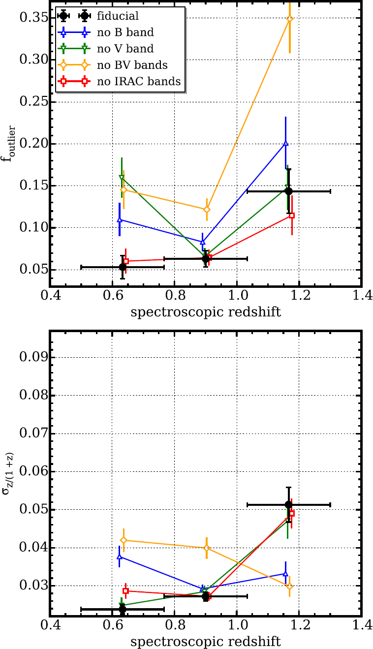
Figure 1: The top panel shows the outlier fraction $f_{outlier}$ in three neighboring redshift regions in SC1604 after removing various bands. The fiducial points refer to no elimination of any band. $f_{outlier}$ here is defined as the fraction of galaxies with $|z_{phot}-z_{spec}|/(1+z_{spec})>0.15$. The bottom panel plots the size of the Gaussian’s standard deviation, $\sigma_{\Delta z}/(1+z_{spec})$. Eliminating both the $B$- and $V$-bands produces the least constrained photometric redshift sample, indicating the necessity of including them.

Since we will eventually be including objects with $z_{phot}$ values in our analysis, we attempted to test the consequence of varying the number of bands and the specific bands in which an object is detected on the accuracy and precision of the recovered $z_{phot}$. This is done in order to limit the final catalog to those objects with higher quality $z_{phot}$ values so as to maximize the purity and completeness of the eventual overdensity candidates that we find. To test this, we compared $z_{phot}$ and $z_{spec}$ values for $\sim$1400 galaxies in one of the ORELSE fields (SC1604) with secure spectral redshifts running EAZY fitting on a variety of different combinations of photometry. In total we tested five cases, i) all photometric data included (fiducial), ii) $B$-band imaging removed, iii) $V$-band imaging removed, iv) both $B$- and $V$-band imaging removed, and v) all IRAC imaging removed. In each case, the $z_{phot}$ values generated from that set of photometry are compared to the $z_{spec}$ values by $\sigma_{\Delta z/(1+z_{spec})}$ and $f_{outlier}$. These results are shown in Fig. 1. We found that removing $B$-band information increases $\sigma_{\Delta z/(1+z_{spec})}$ by over 50% at low redshift as well as drastically increasing $f_{outlier}$. Additionally, $f_{outlier}$ is significantly higher at high redshift when both the $B$- and $V$-band information are excluded. Interestingly, excluding the information from the IRAC bands from our fitting had very little effect on the $z_{phot}$ precision or accuracy relative to the fiducial setup at least for the galaxy population studied here. We chose the IRAC bands for this exercise rather than in the $J/K$ bands because the latter are relatively shallow and cutting on these bands results in fewer total objects remaining to perform this test on. Additionally, we tested the effect of requiring different significance detections in the $B$- and $V$- bands, finding that requiring magnitude errors of $\leq 0.3$ in both bands gave the best combination of precision and accuracy while still allowing us to include most photometric objects in our final sample. This criteria was imposed on all photometric objects to generate our final sample (with the exception of the XLSS005 field, see below) and corresponds to detection significance of $\geq$3.6$\sigma$ in both bands.

In essentially every field, because the $B$- and $V$-band images are deep (see Table 13), and because we include only those objects brighter than $i/z<24.5$ in our final sample, the above criteria essentially amounts to only including those areas where $B$- and $V$-band coverage is available, which is the case for essentially every spectroscopic object. The $B$- and $V$-band requirement additionally included most of the photometric objects in our redshift catalog in the range of 18 $\leq i/z\leq$ 24.5 (Fig. 2). These cuts were used for all spectroscopic and photometric objects in the 14 ORELSE fields that have similar imaging depth in the $B$- and $V$-bands. The one remaining field, XLSS005, has CFHT Legacy Survey (CFHTLS) $u^{*}$/$g^{\prime}$ imaging that acted in place of our typical $B$- and $V$-band requirement (Table 13).

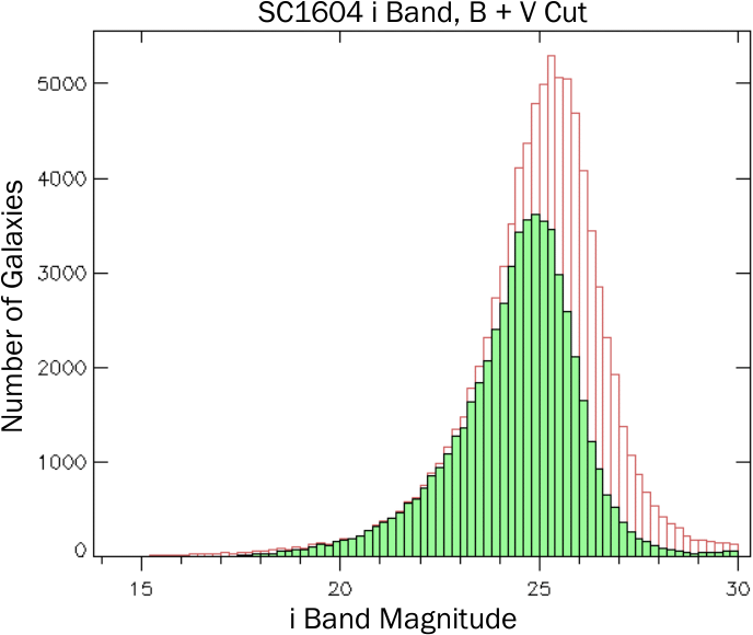
Figure 2: The $i$-band magnitude distribution for all objects in the SC1604 field compared with the population of objects with $B$- and $V$-band photometric errors less than 0.3 mag in green. The $B$ and $V$ cut still contains the majority of objects in the magnitude range of interest, 18 $\leq i\leq$ 24.5.

For the purpose of this work, spectroscopic redshifts are extremely helpful, since they provide highly accurate information on the position of the galaxies along the line of sight and are therefore extremely important in identifying and mapping the large-scale structures. However, obtaining spectra for a large and contiguous field is difficult, and often the spectroscopic coverage is not evenly distributed in the sky (see an example in Fig. 3). This is why our approach in detecting overdensity candidates (see §3) includes the use of both spectroscopic and photometric redshifts. The latter, although less accurate, generally has a more uniform spatial distribution. In conjunction with the spectroscopic redshifts, $z_{phot}$ values, if treated properly, are able to provide a more complete mapping of the density field. As a reminder, however, we limited our sample to areas in and near the spectroscopic footprint, as the effectiveness of our methodology degrades considerably in the complete absence of spectroscopic redshifts.

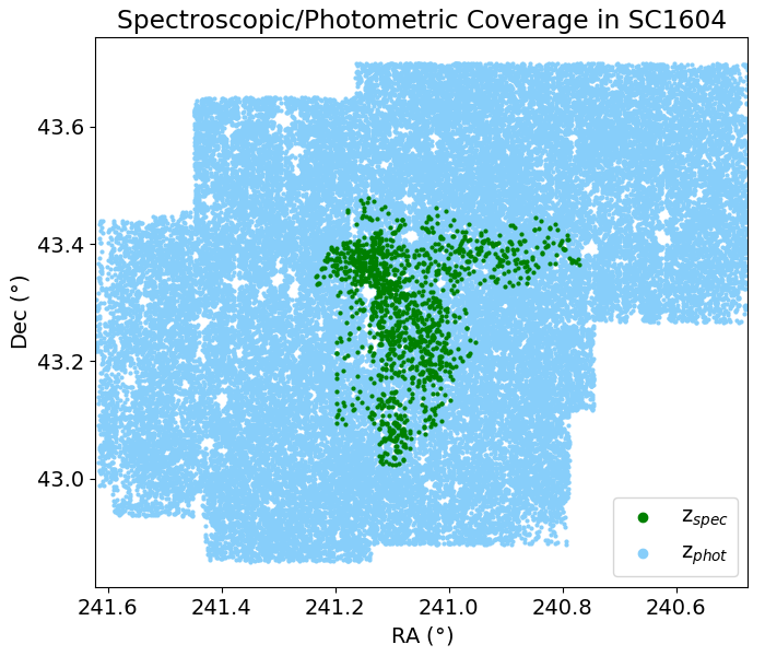
Figure 3: All photometric and high-quality spectroscopic members in the ORELSE field SC1604. The photometric and spectroscopic redshifts in this field cover the ranges $0.03<z_{phot}<5.76$ and $0.11<z_{spec}<2.76$, respectively. Of all the ORELSE fields, SC1604 is the most well sampled field, with high spectroscopic coverage and superb photometric redshift accuracy and precision. The photometric coverage far exceeds the spectroscopic range, which is primarily limited to the regions around the known structures in the field. Regions with no imaging data or with severe issues with bright stars or other imaging artifacts (depicted in white) are masked and excluded from the overdensity calculations of each ORELSE field. We limit our search range to the spectroscopic footprint as overdensity candidates detected outside the spectroscopic range of coverage will likely have more uncertain redshifts than those inside due to the higher uncertainty in the photometric redshifts.

3 Methodology

Our goal is to discover and characterize new overdensity candidates in the ORELSE fields. Once we identify these candidates, we can translate each of their overdensities derived from the VMC overdensity maps to their total gravitating halo mass. This translates the observed spatial clustering of galaxies into a mass distribution, which can be used to trace the underlying dark matter distribution as described in Cucciati et al. (2014). For overdensity candidates with sufficient spectroscopy, we can also estimate masses from their measured velocity dispersions (Gal et al., 2008; Lemaux et al., 2012).

To find new overdensity candidates, we look for overdensities that subtend a large angular distance and are coherent over some redshift range. We apply the standard photometry software package Source Extractor (SExtractor; Bertin & Arnouts, 1996) to the VMC overdensity maps, which are divided into several small redshift slices, to identify overdensities candidates in each slice.

In this section, we describe the methods used in our overdensity candidate detection algorithm. We discuss our optimization schemes and how we set our parameters in §4.

3.1 Voronoi Tessellation

Mapping the density field of galaxies requires a large, homogeneous, and unbiased sample of galaxies with accurate redshifts (spectroscopic and/or photometric, Darvish et al., 2015). 2D surface density estimates are made using a series of narrow redshift slices, where the widths of the z-slices are set at first-order by some characteristic of the data, for example the photometric redshift precision or the redshift extent of structures in the field. A too narrow width might miss galaxies belonging to a structure extended along the line of sight, while a too broad width risks contamination from foreground and background galaxies. We construct our overdensity maps with what is known as the Voronoi tessellation Monte-Carlo (VMC) method. Optimizing our VMC overdensity map code is critical for accurately determining the redshifts of all overdensity candidates in a field.

A Voronoi tessellation is the division of a 2D plane into a number of polygonal regions equal to the number of objects in that plane. The Voronoi cell of each object is defined as the region closer to it than to any other object in the plane. Objects in high density regions therefore have small Voronoi cells, while objects in lower density regions have larger cells. The inverse area of the cell sizes can thus be used to measure the local density at the position of the object bounded by the cell.

When we apply the Voronoi tessellation to our data, the redshift slices are our 2D planes and the galaxies are the objects in the planes. Voronoi tessellation is advantageous to use over other density field estimators as it is scale-independent and can be used over large physical lengths. Most importantly for the detection of often irregularly shaped overdensity candidates, it makes no assumptions about the geometry or morphology of structures in the field (Darvish et al., 2015).

Not all galaxies have equally well-determined redshifts. We must take into account the high uncertainties in using the photometric redshifts. To do so, we use a VMC technique broadly following the weighted Voronoi tessellation estimator method outlined in Darvish et al. (2015) and described in (Lemaux et al., 2018). For the galaxies in our sample with only photometric redshifts, $z_{phot}$, we use a Monte-Carlo acceptance-rejection process to treat these redshifts and their uncertainties from EAZY as statistically asymmetric Gaussians.

For each Monte-Carlo realization, we assign a new $z_{phot,MC}$ to each $z_{phot}$ galaxy. This $z_{phot,MC}$ is randomly sampled from a simplified version of the $z_{phot}$ PDF, where we assume the PDF is a Gaussian centered on the original $z_{phot}$ PDF. The $\sigma$ of the $z_{phot,MC}$ is either the upper or lower $z_{phot}$ error depending on whether the sampled random number was above or below the mean of the Gaussian peak. If the sample point is lower than the mean of the Gaussian peak, it is multiplied by the lower 1$\sigma$ on the galaxy’s $z_{phot}$ and subtracted from the original $z_{phot}$. If the sample point is higher than the mean of the Gaussian peak, it is multiplied by the upper 1$\sigma$ on the galaxy’s $z_{phot}$ and added to the original $z_{phot}$.

These $z_{phot,MC}$ and $z_{spec}$ galaxies are sliced into bins of approximately $\pm$1500 km s^-1 in velocity space over $0.55<z<1.37$. We discuss how we set our number and width of slices in §4.2. The Voronoi tessellation is applied on 100 realizations of each bin. For each realization, a grid of 75$\times$75 proper kpc pixels is used to sample the local density distribution for each slice. The local density of each grid point for each realization is set equal to the inverse of the Voronoi cell area that encloses the grid point, multiplied by the square of the angular diameter distance. As the slices go to higher redshift, the projected size of the sky covers a larger proper area. Because the pixel scale is fixed, this means the image size for each redshift slice will increase with higher redshift for the same field. The final local overdensities for each grid point in the redshift slice are computed by median combining the values from the 100 Monte-Carlo realizations. The local overdensity in a pixel ($i,j$) is approximated with

$$\mathrm{log}(1+\delta_{\mathrm{gal}})=\mathrm{log}(1+(\Sigma_{i,j}-\tilde{\Sigma})/\tilde{\Sigma})$$ (1)

where $\delta_{\mathrm{gal}}$ is the density of galaxies, $\Sigma_{i,j}$ is the given pixel’s density, and $\tilde{\Sigma}$ is the median density of all pixels in the slice (Fig. 4). As discussed in Tomczak et al. (2017); Lemaux et al. (2019), these local overdensities have been shown through tests to correlate well with other density metrics and, as we will show later, trace out the known structures extremely well.

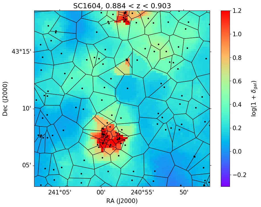
Figure 4: Depicted is a portion of one redshift slice in the Voronoi Monte-Carlo overdensity map around the SC1604 A overdensity with one of the Voronoi tessellation realizations overlaid. Each ORELSE field is sliced into redshift bins of $\Delta\mathrm{v}=\pm 1500$ km s^-1 wide across the redshift range of $0.55<z<1.37$. For each slice, the photometric redshifts are randomly sampled 100 times based on their estimated $z_{phot}$ uncertainties. The black points, or galaxies, in the slice are partitioned into polygonal cells with a single realization of the Voronoi tessellation, where each cell represents the projected area that is closest to the galaxy in it than any other galaxy. The underlying overdensity map, shown in the background, is the median among the 100 VMC realizations, on a grid of 75$\times$75 kpc pixels, as described in the text. The color code is shown in the color bar on the right.

3.2 Source Extractor

We used SExtractor to find the overdensity candidates in our VMC overdensity maps. As clusters and groups are not necessarily regular in shape, we use the isophotal fluxes rather than any of SExtractor’s elliptical or circular apertures. When running SExtractor over a VMC overdensity map, SExtractor outputs isophotal flux values, which are its measure of a given region’s overdensity. Thus, higher fluxes indicate higher densities. SExtractor identifies pixels as significant if their overdensities are above some given detection threshold. The pixels are then identified as detections if their groupings are larger than some given minimum area. The higher the detection threshold and the larger the minimum area, the fewer detections SExtractor will find. Therefore, carefully choosing the optimal parameters is key for finding as many overdensity candidates in the map as possible without being overwhelmed by astrophysical and random noise. We discuss the optimization of these parameters in greater detail in §4.

3.2.1 Linking SExtractor Detections

In order to find significant overdensity candidates in our fields, we must first properly assess the background galaxy density, which is calculated by SExtractor. The outer edges of the imaging footprint in the VMC overdensity maps have higher galaxy incompleteness and thus artificially low overdensities. Including such regions in our SExtractor analysis would skew the average background galaxy overdensity low. When the VMC overdensity maps are made, we compute the densities after masking out regions without imaging data or which have been severely corrupted by bright stars or image artifacts, and then calculate the overdensities. In the final overdensity maps, we still have low density regions around the boundaries of the imaging footprint. To exclude these low density regions, we constructed a mask for every redshift slice in each field to remove the areas of the maps with overdensities less than log(1+$\delta_{gal}$) = -0.35 and passed them into SExtractor. Over all ORELSE fields, this masked roughly 5.8% of the spectroscopic footprint, but 0% of the spectroscopic footprint of five fields: SG0023, SC0849, RXJ1053, Cl1350, and SC1604.

For every redshift slice, SExtractor outputs a position and total isophotal flux for each detection it finds. To find coherent overdensity candidates across separate redshift slices, we calculate the distances between all SExtractor detections in one slice with all SExtractor detections in the immediate next redshift slice. The distance calculated is the angular diameter distance evaluated at the redshift which is the average of the two slices’ central redshifts.

If two detections are within a certain linking radius, we consider them as part of the same overdensity candidate. We then use their flux weighted position to attempt to link the pair with a third detection in the next redshift slice, where the link is successful if the third detection is also within the same linking radius as before. This process is repeated across redshift slices until no further links are found. The final centroided position is the flux weighted average of all linked detections in that overdensity candidate. Further details of this search and our tests with different linking radii can be found in §4.2.

The redshift of the overdensity candidate is then determined by fitting a Gaussian to the isophotal fluxes of all the linked detections as a function of redshift, where the isophotal flux and error for each detection are calculated by SExtractor. We use the standard deviation of the Gaussian, $\sigma_{z}$, to describe the redshift dispersion. We expect the redshift of a overdensity candidate to be where the density of galaxies is highest, and we take the mean of the Gaussian fit to be the redshift of the overdensity candidate (Fig. 5). To avoid cases where the Gaussian is largely extrapolated and fitted only to a few data points near one tail, we require the amplitude of the Gaussian to be no more than 20% of the highest value data point in the fit and remove all candidates that do not meet this criterion.

Because we attempt to link all possible SExtractor detection chains starting at each redshift slice, there will be some linked overdensities which are subsets of links that begin at earlier redshifts. However, these overdensities will likely have similar redshifts and centroided positions. We control for these duplicate detections by iterating over all the detections in a field, starting from the largest Gaussian fits by amplitude, and removing any other detections within both 0.7 Mpc, a distance which is the average extent of a group or cluster, and $\Delta z<0.02$. There will likely be a few duplicate detections of the more irregularly shaped overdensities remaining after this removal process, but we expect these to be few in number. We go over the results of setting this separation threshold in §6.

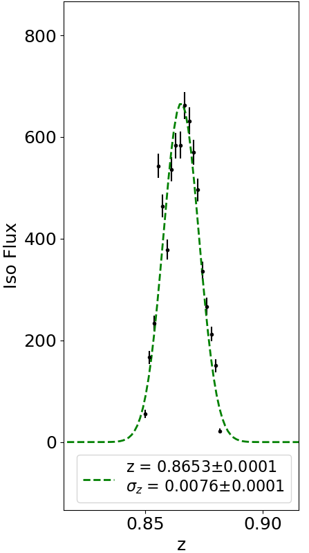
Figure 5: The panel shows an example of a Gaussian fit of a linked overdensity candidate. The individual points are the isophotal flux values of individual SExtractor detections in neighboring redshift slices. The position of the overall overdensity candidate is an average weighted by the isophotal flux of all linked detections in the overdensity candidate. $\sigma_{z}$ is the redshift dispersion, describing the width of the Gaussian fit and therefore the extent of the overdensity candidate across redshift.

4 Optimization and Choice of Parameters

4.1 Detection Parameter Optimization

SExtractor’s object identification strongly depends on the choice of DETECT_THRESH, the detection threshold significance above the median overdensity, and DETECT_MINAREA, the minimum area of an object in square pixels. The isophotal fluxes calculated by SExtractor are the overdensities above the detection floor. A higher floor in other words translates to smaller isophotal fluxes. Too restrictive parameters means we lose detection of structures, but too inclusive parameters inundates our identified overdensity candidates with noise and false detections. Larger minimum areas require the detection of more of an overdensity candidate’s subtended angular size, lowering the chance of a false positive detection, but can miss detecting lower mass clusters. Smaller areas only require detecting overdensity cores but are more susceptible to noise contamination.

We tested a grid of DETECT_THRESH of 3, 4, 5, and 6$\sigma$ and DETECT_MINAREA of 10, 20, 40, 80, and 160 square pixels. The $\sigma$ value is what SExtractor calculates as the RMS noise in the background of a given slice of the VMC overdensity map. For a single detection, all the pixels must be above the detection threshold and adjacent to each other, and the total area of the pixels must be at least as big as the minimum area. Ideally, we should set our detection threshold low enough to pick up groups and low mass clusters but not so low that we are overwhelmed by small fluctuations of noise. The results of these tests are detailed in §4.3.

We did not use any smoothing Gaussian filter in SExtractor as filters are best suited for recovering regularly shaped large-scale structures, and real structures are not necessarily all regularly shaped. We did test how various filtering schemes performed when attempting to recover injected mock structures in §5.2 and found only a very modest improvement when using a filter versus not using a filter at all.

We found the background RMS values in our fields were generally around $\log(1+\delta_{gal})$ = 0.09-0.15. Our grid of detection threshold $\sigma$s probe below and above a local overdensity of log(1+$\delta_{gal}$) = 0.5, which is the typical high end of the $\log(1+\delta_{gal})$ distribution for field surveys and likely corresponds to group-like environments (Pelliccia et al., 2017). The minimum area is essentially a measure of the velocity dispersion of a structure. Smaller minimum areas are sensitive to smaller velocity dispersions. The velocity dispersions of clusters are typically calculated over a 0.5 or 1 Mpc radius. With our 75$\times$75 proper kpc pixel scale, our minimum areas cover the lowest end of this range, translating to circles with areas of 0.06 to 0.9 square Mpc, which allows us to more easily identify groups and low mass clusters.

4.2 Linking Detections Across Redshift Slices

As first introduced in §3.1, we tested using VMC overdensity maps divided into redshift slices of different spacings. With more overlap between neighboring slices, we have more total redshift slices and thus a higher number of detections of a overdensity candidate in the field. We expect the overdensity candidates will be easier to detect with more detections, though increasing the total number of redshift slices can greatly increase the total computation time in constructing the VMC overdensity maps.

When constructing our VMC overdensity maps, we set our redshift slice size at 0.01(1+z), corresponding to an approximately $\pm$1500 ${\rm km~{}s^{-1}}$ velocity dispersion. This value is roughly twice the typical velocity dispersions for known structures in the ORELSE fields and rivals the velocity dispersions observed for the most massive galaxy clusters (e.g., Ruel et al., 2014; Owers et al., 2017). With narrower redshift slices, we run the risk of subsampling structures, missing massive cohesive structures because they could become separated over different bins. The same is true for galaxies with only photometric redshifts, as these redshifts have much coarser resolution than z $\sim$ 0.01. We tested using redshift slice sizes two and four times bigger than 0.01(1+z) and found that these wider slices placed a majority of distinct redshift structures into the same redshift slice, reducing the accuracy of their measured redshift. Additionally, instituting wider bins had the effect of several of the known ORELSE structures being missed entirely since their full redshift extent were fully contained in only one slice.

The VMC overdensity maps are made such that each redshift slice deliberately overlaps with the slice before it. This avoids scenarios where a single overdensity candidate gets separated over different slices. We tested maps where the overlapping redshift slices were centered at $\Delta z$ step sizes of 1/3, 1/4… 1/10 of the total width of each slice. In other words, at a 1/10 step size, we would for example have neighboring redshift slices covering $z$ = 0.600 to 0.620 and $z$ = 0.602 to 0.622, or 90% overlap between the two slices. The width of the redshift slice remains the same regardless of the step size.

We tested how well linking radius values, as described in §3.2.1, of 0.25, 0.5 and 1 Mpc performed in recovering three known structures in SC1604 at around $z\sim 0.9$, Clusters A, B, and D. We chose the SC1604 field because, of all the fields in ORELSE, SC1604 is the closest to being ideal for such a test in several regards. It is the field in ORELSE with the most dense spectroscopic coverage, and as well as some of the deepest. In addition, the large number of bands and the depth of the imaging have resulted in excellent $z_{phot}$ accuracy and precision. We selected Clusters A, B, and D in this field for our tests because they are large and isolated, and they spanned a narrow redshift range, so we could construct VMC overdensity maps for these tests in a relatively short time-frame. These structures additionally span a range of different morphologies, where Cluster A appears as a typical cluster, Cluster B is close to dynamically relaxed, and Cluster D is elongated and irregular in shape (see Lemaux et al. 2012; Rumbaugh et al. 2018 for more details). We found that a 1 Mpc linking radius was the only value large enough to link detections over the full Gaussian profile for Cluster D. The 1 Mpc linking radius also performed best overall in recovering the fiducial redshifts (Fig. 6). The fiducial redshifts were taken from the biweight mean of the known spectral members, which were within 3$\sigma$ of the LSS’s velocity dispersion and a 1 Mpc projected radius.

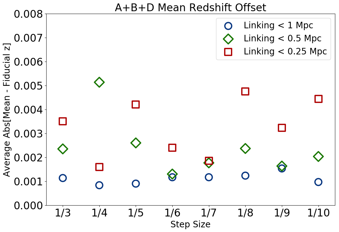
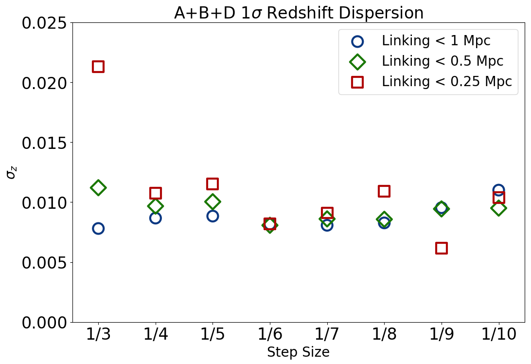
Figure 6: The average absolute offset between the fiducial and fitted mean redshifts and 1$\sigma$ redshift dispersions $\sigma_{z}$ for known Clusters A, B, and D in SC1604. The step size is the spacing between redshift slices set as a fraction of the total width of each slice. The largest linking radius of 1 Mpc performs the best in recovering the fiducial redshifts. The redshift dispersions are all on the order of 0.01 for every linking radius, showing that we consistently recover the shape of each structure well. We find no significant dependence on step size for either the determined mean redshift or redshift dispersion.

The spectroscopic coverage in each ORELSE field is not uniform. Our densest spectroscopic coverage is around known structure targets. Many of the overdensity candidates in the field are likely to be less spectroscopically sampled. As a cursory estimation on how well our large-scale structure detection algorithm performs for such cases, we also test how well we can recover the known structures using smaller fractions of the spectroscopic data available. We thus repeated the same step size tests with SC1604 using 50% and 25% of the available spectroscopic redshifts in constructing the VMC overdensity maps. Decreasing the number of spectroscopic members is a good approximation for how our large-scale structure detection algorithm would fare with the overdensity candidates we are trying to find, as they generally will have lower levels of spectroscopic completeness than the nearly complete ($i\leq$ 24.5) SC1604 field.

When we dropped the fraction we used of our available spectroscopic data, we found that there was a greater chance of losing overdensity candidate detections with a step size larger than 1/10, as we missed the detection of Cluster D in our tests at 50% (where the detection is lost at 1/3 and 1/6 step sizes) and 25% (where the detection is lost at 1/8 step size) of the spectroscopic data used. That we still successfully detect Cluster D with some smaller step sizes can be attributed to the small number statistics in these tests. However, having any missed detections at all implies that smaller step sizes are necessary for maximizing overdensity candidate detection completeness for less spectroscopically complete fields, especially for those of irregular shapes. The difference between the measured mean redshift and the fiducial redshift also generally increased with smaller fractions of spectroscopic data used, though even the largest difference we found was still very small. The redshift dispersions are consistently on the order of $\sigma_{z}\backsim$ 0.01 regardless of step size, demonstrating how well we can recover the shape of structures when we do detect them (Fig. 7).

We thus elected to adopt a step size of 1/10, which means that adjacent redshift slices have 90% overlap, for constructing the VMC overdensity map for the entire redshift range, so as to maximize our chances of successful overdensity candidate detections. To cover our entire redshift range of $z$ = 0.55 to 1.37 for our serendipitous overdensity candidate search, this translates to using 420 redshift slices for each field.

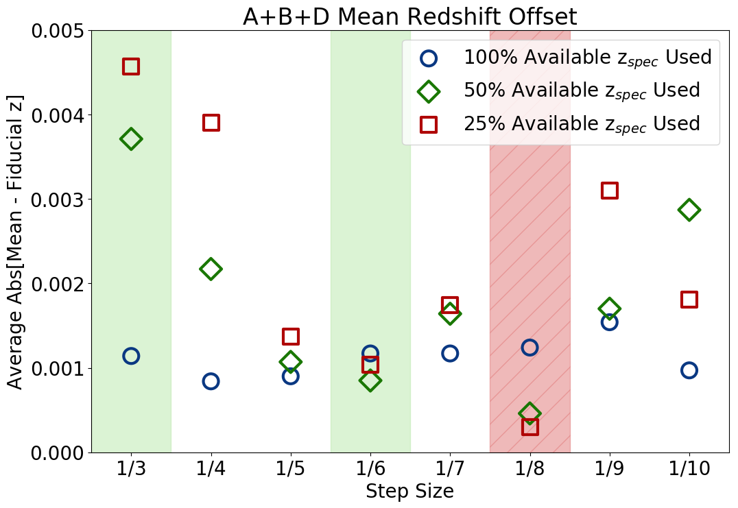
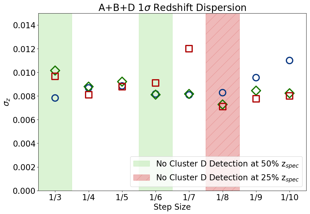
Figure 7: Average absolute mean redshift offset and 1$\sigma$ redshift dispersions for Clusters A, B, and D using varying fractions of the available spectroscopic redshifts using a linking radius of 1 Mpc. The offset generally worsens with smaller fractions of spectroscopic data used, though even the maximum offset is still very small. The dispersions are consistently on the order of $\sigma_{z}\backsim$ 0.01, demonstrating how well the VMC method can recover the shape of the structures when only those objects with photometric redshifts that include significant detections in the $B$ and $V$ band even when a large percentage of the spectral redshifts are removed. The detection of Cluster D is lost at 1/3 and 1/6 step sizes for 50% of the spectroscopic data used, and at 1/8 for 25%. Though these tests operate at the mercy of small number statistics, having missed detections at all suggests that smaller step sizes are necessary to maximize overdensity candidate detections for less spectroscopically complete fields.

4.2.1 Determining the Background RMS

The background RMS value is critical for setting the detection threshold. When we pass our VMC overdensity maps to SExtractor, it estimates the background of the image and the RMS noise in that background. SExtractor computes the mean and standard deviation of the pixel value distribution in a 64 square pixel area. It then discards the most deviant and computes the mean and standard deviation again. This process is repeated until all the remaining pixel values are within 3 standard deviations of the mean.

As mentioned in §3.2.1, we masked regions of the VMC overdensity maps with overdensities less than log(1+$\delta_{gal}$) = -0.35 in order to facilitate the accuracy of SExtractor’s background RMS calculation. SExtractor excels in cases where the detections it finds are much smaller than the image containing them. This is not the case for many of our fields. We found that large-scale structures present in a field will often vary the field’s background RMS as a function of redshift by more than 50% higher than its mean value, clearly indicating that SExtractor had confused overdensity candidates for background. This effect is most prominent in RXJ1821, where a single large structure at $z$ = 0.8168 quadrupled the mean background RMS value.

There was additionally a persistent stochasticity in the background RMS as a function of redshift. The difference in the background RMS measured in neighboring redshift slices often exceeded the mean background RMS over the entire redshift range of the field. This variation in the background RMS is minimal for SC1604 and XLSS005, which are the targets with the largest imaging fields of view relative to the spectral footprint and the sizes of the structures, in contrast to smaller fields such as Cl1429 or RXJ1821.

Due to the background RMS variations between fields, we would find structures of similar velocity dispersions with systematically smaller or larger isophotal flux peaks between fields of similar imaging depths, such as structures in SC1324 having much smaller peaks than SC1604. Because the detection threshold is set as a multiple of the background RMS, the higher background RMS in SC1324 compared to SC1604 meant that the former had an effectively higher threshold for the same relative DETECT_THRESH value. For example, using a DETECT_THRESH parameter of 4$\sigma$ would measure a smaller isophotal flux for an overdensity candidate of the same mass, velocity dispersion, and overdensity in SC1324 than it would in SC1604. This implied that the discrepancies we were finding arose due to how the data analysis was performed rather than an inherent characteristic of the structures in different fields.

To allay the stochasticity of the background RMS between neighboring redshift slices, we fitted each field’s RMS as a function of redshift with a fifth order polynomial. We used the RMS of that fit to identify outliers greater than 3$\sigma$ away from the value predicted by our polynomial fit and then fitted the background RMS again without the outliers. We performed this outlier rejection iteratively, repeating until the polynomial fit found no more outliers at above 3$\sigma$, which is similar to the methods adopted by Cucciati et al. (2018). In the majority of fields, the fit with outlier rejection was largely unchanged from the first fit, only noticeably deviating in fields with large peaks in the background RMS values (Fig. 8). We use these polynomial fits to set the RMS as a function of redshift in each ORELSE field in SExtractor.

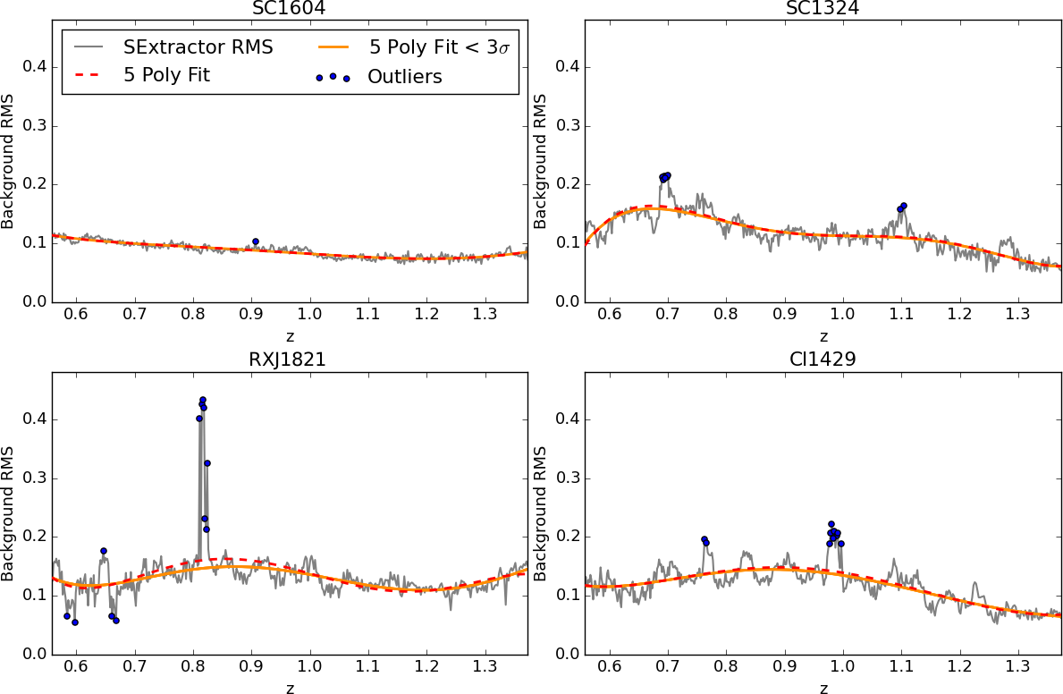
Figure 8: The background RMS as a function of redshift in four fields, SC1604, SC1324, RXJ1821, and Cl1429. The gray lines are the background RMS as calculated by SExtractor. The dashed red line represents a fifth order polynomial fit without outlier rejection. The solid orange line represents a fifth order polynomial fit with iterative outlier rejection at above 3$\sigma$, based on the RMS of the preceding polynomial fit. The difference between the two fits with and without outlier rejection is largely minimal outside of areas with large peaks in the background RMS values. SC1604 is a very large field with deep imaging and shows a very flat RMS curve while Cl1429 sees a much more variation in its RMS as a function of redshift. SC1324 and RXJ1821 show noticeable peaks at redshifts of 0.7 and 0.8 respectively, which correspond to known large structures in each field.

4.3 Recovering Known Structures

As a preliminary test of overdensity candidate completeness for different levels of spectroscopic coverage, we looked to see how well our choice of SExtractor parameters would recover 22 different known clusters and groups in ten ORELSE fields, which visually appeared to be isolated from other systems in the fields (Table 2). We refer to these hereafter as “isolated structures.” This additionally tests our sensitivity to low mass structures as some of these structures have virial masses as low as 3-4$\times$10¹³ M_⊙, on par with that of the Local Group. Virial masses are computed based off the velocity dispersions $\sigma_{v}$ that we measured using the spectroscopic data, using the formula in Lemaux et al. (2012):

$$M_{vir}=\frac{3\sqrt{3}\sigma_{v}^{3}}{11.4\mathrm{G}\mathrm{H(z)}}$$ (2)

where G is the gravitational constant and $H(z)$ is the Hubble parameter. A structure’s velocity dispersion is calculated using number of spectroscopic members in the structure, following the methods described in Rumbaugh et al. (2013) and Ascaso et al. (2014). The velocity dispersion is calculated from the galaxies which make up the structure, and the galaxy membership is determined using an iterative process. Galaxies are initially identified as part of a structure if they fall within a 1 Mpc radius of the structure’s density peak and then iteratively clipped for 3$\sigma$ outliers. Detections in the VMC overdensity maps were linked with known structures if their determined redshift was within $\Delta z<0.02$ of their previously reported redshift and was centroided within 1 Mpc of their reported coordinates. We discarded all detections we found which had $\sigma_{z}>0.05$, or a velocity dispersion of around $\pm$6000 km s^-1, as such systems would be unphysically large.

Table 2: Selected Isolated ORELSE Galaxy Clusters and Groups

Structure	Redshift	RA (J2000)	Dec (J2000)	Membersa	$\sigma_{v}$b	log(Mvir)c
SC1604 Lz	0.5995	241.03282	43.2057	21	771.9 $\pm$ 110.0	14.711 $\pm$ 0.186
SC1604 A	0.8984	241.09311	43.0821	35	722.4 $\pm$ 134.5	14.551 $\pm$ 0.243
SC1604 B	0.8648	241.10796	43.2397	49	818.4 $\pm$ 74.2	14.722 $\pm$ 0.118
SC1604 G	0.9019	240.92745	43.403	18	539.3 $\pm$ 124.0	14.169 $\pm$ 0.300
SC1604 H	0.8528	240.89890	43.3669	10	287.0 $\pm$ 68.3	13.359 $\pm$ 0.310
SC1604 Hz	1.1815	241.07967	43.3215	15	661.5 $\pm$ 80.2	14.367 $\pm$ 0.158
SC1324 A	0.7566	201.20129	30.1924	43	873.4 $\pm$ 110.8	14.833 $\pm$ 0.165
SC1324 H	0.6990	201.2204	30.8408	19	346.4 $\pm$ 109.8	13.708 $\pm$ 0.393
SC1324 I	0.6956	201.2055	30.9665	35	847.1 $\pm$ 96.4	14.808 $\pm$ 0.148
SC0849 A	1.2637	132.23463	44.76178	13	714.4 $\pm$ 171.6	14.448 $\pm$ 0.313
SC0849 D	1.2703	132.14184	44.896338	23	697.2 $\pm$ 111.2	14.415 $\pm$ 0.208
SC0849 E	1.2601	132.27496	44.959253	14	445.1 $\pm$ 71.9	13.833 $\pm$ 0.210
RCS0224 A	0.7780	36.15714	-0.0949	34	825.4 $\pm$ 193.2	14.754 $\pm$ 0.305
RCS0224 B	0.7781	36.14123	-0.0394	52	710.7 $\pm$ 58.8	14.559 $\pm$ 0.108
RXJ1221 B	0.7000	185.34103	49.3138	18	426.6 $\pm$ 71.3	14.654 $\pm$ 0.222
RXJ1053	1.1285	163.43097	57.591476	28	898.0 $\pm$ 142.0	14.778 $\pm$ 0.206
RXJ1053 Hz	1.2000	163.20387	57.58400	11	916.3 $\pm$ 194.8	14.786 $\pm$ 0.277
RXJ1821	0.8168	275.38451	68.465768	52	1119.6 $\pm$ 99.6	15.227 $\pm$ 0.218
RXJ1757	0.6931	269.33196	66.525991	34	862.3 $\pm$ 107.9	14.832 $\pm$ 0.250
Cl1137	0.9553	174.39786	30.008930	28	534.6 $\pm$ 81.1	14.144 $\pm$ 0.197
RXJ1716 B	0.8092	259.21686	67.139647	83	1120.6 $\pm$ 101.5	15.145 $\pm$ 0.118
RXJ1716 C	0.8146	259.25725	67.152497	39	678.4 $\pm$ 57.8	14.489 $\pm$ 0.111

$a$: Number of galaxy members used for the velocity dispersion calculation within a 1 Mpc radius.

$b$: Velocity dispersion in ${\rm km~{}s^{-1}}$ within a 1 Mpc radius.

$c$: Virial mass in units of solar mass, calculated from the formula given in Lemaux et al. (2012).

Selected isolated known structures across 10 ORELSE fields used to test our detection threshold parameters. Though this table lists 22 structures, we effectively have 20 as we treat Clusters A and B in RCS0224 and B and C in RXJ1716 as single structures, with their redshifts, positions, and velocity dispersions member-weighted between each pair of clusters. The number of galaxy members, central positions, and velocity dispersions are calculated using the methods described in Rumbaugh et al. (2013) and Ascaso et al. (2014).

As stated in §4.1, we tested a grid of parameters in SExtractor of DETECT_THRESH of 3, 4, 5, and 6$\sigma$ and DETECT_MINAREA of 10, 20, 40, 80, and 160 square pixels. We tested these parameters in conjunction with using 25%, 50%, 75%, and 100% of the available spectroscopic redshifts similar to what we did earlier in §4.2. For any percentage of $z_{spec}$ members, we looked for which pair of parameters would recover the highest percentage of our subset of known isolated structures. We found that generally the differences due to the choice of different minimum areas were small compared to those due to the choice of different detection thresholds, and similar minimum areas for a given detection threshold produced identical results.

Detection thresholds of 5 and 6$\sigma$ often were not able to find any of the known isolated structures nor produce any other overdensity candidates. This effect was more pronounced at smaller fractions of spectroscopic redshifts used. The 3$\sigma$ detection threshold also lost several detections of our lower mass structures at smaller spectroscopic fractions that were found by the 4$\sigma$ threshold, indicating the 3$\sigma$ threshold did not sufficiently filter out noise in the VMC maps. The 3$\sigma$ threshold additionally more poorly centroided the positions of the known structures it found compared with the 4$\sigma$ threshold. As the majority of these structures have high $z_{spec}$ fractions, we expect their fiducial positions to be highly accurate, so the centroid offsets are generally meaningful. From these results, we concluded it was best to use a 4$\sigma$ detection threshold (Fig. 9).

Figure 9: The recovered fraction of known structures in Table 2 based on different detection threshold (D, in units of $\sigma$, given on the top axis) and minimum area (A, in pixels, given on the bottom axis) parameters as well as fraction of available spectroscopic redshifts used in constructing the VMC maps. A known structures is considered successfully recovered if it lies within $\Delta z$ = 0.02 of the nominal redshift and 1 Mpc of the nominal central coordinates. We found that a 4$\sigma$ detection threshold was able to recover more structures at lower spectroscopic completeness.

For a 4$\sigma$ detection threshold, minimum areas of 10 and 20 pixels were able to recover the most isolated structures for all fractions of spectroscopic redshifts, with a difference in redshift offset within z $<$ 0.001. The 10 pixel area had a better positional centroid in every case but at 50% available $z_{spec}$ used, where the 10 pixel area has the advantage of recovering one structure that the 20 pixel area did not find (Fig. 10). The redshifts we determine for the known structures we recover agree very well with their fiducial values, with differences on the order of $\sigma<$ 0.001. This is an order of magnitude more precise than the $z_{phot}$ errors, which are typically on the order of $\sigma\backsim 0.02(1+z)$.

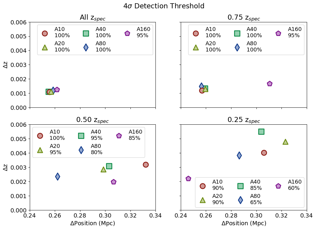
Figure 10: The average absolute offset in redshift and position for all detected isolated structures using a 4$\sigma$ detection threshold with minimum areas (A) of 10, 20, 40, 80, and 160 square pixels. The annotated number next to each point represents the total fraction of the 22 known structures detected. In the top right panel, the 20 and 40 pixel points are overlapping. The 10 and 20 pixel areas recover the most known structures, reaching a minimum of 90% at 25% available $z_{spec}$ used. The difference in the redshift offset between 10 and 20 pixels is within z $<$ 0.001, but the 10 pixel area generally recovers more accurate structure positions while finding as many or more structures than the 20 pixel area.

4.3.1 Deblending Parameters

We often find large overdensities that are in actuality multiple structures in close proximity. To split such overdensities into their component objects, SExtractor uses two deblending parameters, the number of deblending sub-thresholds DEBLEND_NTHRESH and the minimum contrast DEBLEND_MINCONT. SExtractor first defines a number of levels from the detection floor to the peak of the detection. This number is set by the DEBLEND_NTHRESH parameter and the levels are spaced exponentially. SExtractor builds a tree out of a detection, checking each level from the bottom up and branching every time it finds pixels above a threshold separated by pixels below it, similar to using cross-sections of a mountain to identify its peaks.

DEBLEND_MINCONT is the fraction of the overdensities in a peak over the total overdensities in the entire structure. The smaller the minimum contrast, the smaller the peaks can be to be treated as single objects. Setting the deblending too coarse will lose out on detecting overdensity candidates, but too fine parameters will split individual overdensity candidates apart.

Once we settled on the detection parameters to use on the real data, we moved on to selecting the choice of deblending parameters. To do so, we qualitatively assessed how well we recovered structures close in proximity for five fields: Cl1350 at $z$ = 0.80, RCS0224 at $z$ = 0.78, RXJ1716 at $z$ = 0.81, SC1604 at $z$ = 0.90 and 0.93, and SG0023 at $z$ = 0.84. At these redshifts, there were the following numbers of known structures in each field: 3 in Cl1350, 2 in RCS0224, 3 in RXJ1716, 6 in SC1604, and 5 in SG0023.

We tested DEBLEND_NTHRESH values of 16, 32, and 64, and DEBLEND_MINCONT of 0.01, 0.001, 0.0001, and 0.00001. We found that a DEBLEND_NTHRESH of 32 and MINCONT of 0.01 performed the best overall, missing only SG0023 A (a group with mass log(M_vir) = 13.836) and failing to deblend RXJ1716 B and C (clusters with centers 32 Mpc apart). Finer deblending parameters that could recover these clusters split the individual structures in other fields into multiple objects. Though our choice of deblending parameters cannot separate extremely close systems like RXJ1716 B and C, we are able to distinguish structures such as the components of the SC1604 supercluster and even closer systems like RCS0224 A and B. Our technique is able to find overdensity candidates, but for a more rigorous extraction of individual components, we encourage the reader to seek another more specialized technique, e.g., Golovich et al. (2019).

5 Tests with Mock Catalogs

There are limitations to what we can test with the real data. Even with the availability of highly precise spectroscopic redshifts, projection effects can still complicate overdensity detection (Lucey et al., 1980). Many of our observational tests lack a definite truth to compare with, which is an advantage using mock data can provide. In order to assess the purity and completeness of the new overdensity candidates we found using our detection algorithm, we tested how well it performed on mock structures across a range of numbers of members and velocity dispersions and at varying levels of spectroscopic coverage.

5.1 Mock Galaxy Generation

We generate the mocks by first populating a given volume with a population of field galaxies and then injecting galaxy clusters and groups. To simplify the distribution of the field galaxies in our mocks, we drew them from ORELSE fields where we did not find any structure candidates at the redshift of interest and also had deep enough imaging in the relevant bands such that it included a complete sample of galaxies to the magnitude limit given below (see Tomczak et al. 2017 for more details on the completeness limits of our imaging).

We drew the field galaxies for our mocks from the galaxies in SC0849 for $z$ = 0.8 and in RXJ1716 for $z$ = 1.2, using their $z_{phot}$ values to set the line-of-sight dimension and their positions to set the transverse dimension. We chose these two fields as they did not have any overdensity detections in our earlier findings, and being pseudo-realistic, they include an inherently more accurate distribution of galaxies that follows the two-point correlation function. The galaxies we included in these fields were within $\Delta z_{phot}\leq$ 0.025 of the target redshift. When selecting what field galaxies to use, we limited the magnitude range to between 18 and 24.5, using the Subaru $i$-band for SC0849 and the LFC $z$-band for RXJ1716. The field galaxies we use at each redshift cover similarly sized areas of 0.168 and 0.174 square degrees respectively, which are typical of the sizes of the fields in the ORELSE data.

We additionally attempted an alternative arrangement of the field galaxies to see if it would meaningfully change our results. For this method, we use a random distribution to populate the mocks with the same number of field galaxies over the same transverse area as in the pseudo-realistic fields. The line-of-sight dimension was covered with a random uniform distribution within $\Delta z_{phot}<0.025$ of the central redshift of the mock. We compare this random distribution of field galaxies to the pseudo-realistic distribution drawn from SC0849 and RXJ1716. We found no significant difference between the random and pseudo-realistic fields but elected to use the latter in the mocks due to the more representative galaxy distribution.

5.1.1 Field Galaxy Generation

We generate the magnitude distributions of the field galaxies in our mock catalogs according to what is predicted by the Schechter function, using the rest-frame $M_{1700}$ luminosity function parameters from Hathi et al. (2010) for both z $<$ 1 and z$>$1, which are modulated based on the average $M_{B}-M_{FUV}$ colors of galaxies at this redshift. The resulting $M_{*}$ values are consistent with the rest-frame $B$-band luminosity function parameters of Giallongo et al. (2005), and thus our results would be unchanged were we to adopt their parameters. We set a floor for the Schechter function such that we do not sample at luminosities $<0.1L_{*}$.

We allow samples from $0.1L_{*}$ to $10L_{*}$ at redshifts $z\sim 0.8$ and 1.2, as the rest-frame $B$-band is approximately the observed-frame $i$-band at $z\sim 0.8$ and very close to the $z$-band at $z\sim 1.2$. This matches the magnitude range 18 $<i<$ 24.5 we cover with the galaxies in our real data. The redshift range is limited to $\Delta z$ = 0.05 around each target redshift, and this small range is to limit the effect of k-corrections of the galaxies when transforming the $B$-band rest-frame luminosities to the observed-frame $i$-band apparent magnitudes at $z\sim 0.8$ and $z$-band at $z\sim 1.2$. For the mocks at $z\sim 1.2$, we modify the $M_{*}$ parameter to be 1.35 magnitudes brighter than the Hathi et al. (2010) value in order to transform it to the observed $i$-band. This value is supported by the average colors at this redshift range, where the average $M_{B}-M_{FUV}$ color is 1.1 from ORELSE photometric catalogs and the average $M_{FUV}-M_{NUV}$ color is 0.25 as determined by fits to the COSMOS $z_{spec}$ catalogs for galaxies in this redshift range (Lemaux et al., 2019).

5.1.2 Mock Structure Makeup

We inject groups and clusters by drawing galaxies from a Gaussian distribution with a $\sigma$ equal to a velocity dispersion chosen randomly to fit in the range of velocity dispersions we see in known structures. We use the same distribution of field galaxies in each mock for each redshift, and we inject different arrangements of mock groups and clusters over the field galaxies. We inject the mock groups and clusters at the central redshift for each of our two fields, with their centers forced to be within the central 50% region of the mock field. We impose this constraint so that we can mask the outer 20% region of the field when running our detection algorithm. This is to avoid picking up high overdensities due to edge effects from our field galaxy population while avoiding masking out mock cluster and group galaxies. This is effectively already done in the real data because each field is targeted such that the structures are in the center of the imaging footprints. We construct a corresponding VMC overdensity map for each arrangement of mock groups and clusters, and we then use the same detection and identification techniques as in §4.3.

5.1.3 Using Real Data to Set Structure Membership

We would like the mock groups and clusters to have similar numbers of members as our known groups and clusters had in all of the ORELSE fields. In an attempt to constrain the number of spectroscopic and photometric members in the ORELSE groups and clusters, we begin by estimating from the data the true number of members within a virial radius, $R_{vir}$, for each known cluster and group. $R_{vir}$ is defined as:

$$R_{vir}=\frac{\sqrt{3}\sigma_{v}}{11.4H(z)}$$ (3)

where z is the systemic redshift of the cluster, $\sigma$ is the line-of-sight galaxy velocity dispersion for all galaxies within a projected radius of 1 Mpc of the luminosity-weighted spectral member center, and H(z) is the Hubble parameter. See Lemaux et al. (2012) and references therein for details on this definition of $R_{vir}$, the measurement of $\sigma$, and the measurement of luminosity-weighted spectral member centers for ORELSE groups and clusters. Though other definitions of $R_{vir}$ are likely more well-motivated from theory (see, e.g., discussion in §4.1 Cucciati et al. 2018 where $R_{vir}$ is defined to be $\sim$20% larger), we adopt this value of $R_{vir}$ for consistency with previous ORELSE studies. In practice, since we do an aperture correction later in this section, and because we do not use $R_{vir}$ elsewhere, our results are unchanged if we instead adopt another definition of $R_{vir}$.

The initial pool of possible $z_{spec}$ members have redshifts corresponding to peculiar velocities which are at most three times the velocity dispersion of the parent cluster or group, and their projected distances are within the virial radius. For every object in the magnitude range without a secure spectral redshift, we assign the $z_{phot}$ as measured by prior EAZY fitting. Objects within $R_{proj}\leq R_{vir}$ and which have a $z_{phot}$ in the range $z_{min}-\sigma_{\Delta z/1+z}(1+z)<z<z_{max}+\sigma_{\Delta z/1+z}(1+z)$, where $z_{min}$ and $z_{max}$ are the minimum and maximum redshift bounds for spectral membership set by the criterion above, are considered $z_{phot}$ members.

The number of galaxies counted above still may contain contamination from foreground and background galaxies. We thus need to estimate the number of these interlopers and remove them. For every cluster and group for which we performed this estimate for, we chose an area of the imaging which did not to the best of our knowledge contain any large-scale structure or considerable photometric masking. The estimate of the number of contaminating objects, hereafter called $z_{phot,background}$, was performed by measuring the the number of objects within the same photometric redshift and projected spatial range as $z_{phot}$ members at a location on the sky where no cluster or group was detected. In order to futher mitigate any chance at contamination of $z_{phot,background}$ by large-scale structure features surrounding known clusters and groups, the number of objects was estimated at a redshift slightly higher ($\Delta z=0.03$) than the systemic redshift of the cluster or group being measured. The number $z_{phot,background}$ objects for each cluster/group was estimated from estimates in the corresponding field in which it was observed to compensate for field-to-field variance in $z_{phot}$ accuracy/precision.

We then apply the magnitude cut to both of these pools in the relevant band for the particular field, limiting the galaxy samples to objects brighter than 24.5. The total members where the projected radius is smaller than $R_{vir}$ are then the members with the background objects subtracted out, i.e., $N_{mem,R_{vir}}=z_{spec,members}+z_{phot,members}-z_{phot,background}$.

Finally, to approximate the true number of members, $N$, for each group/cluster, the above numbers are aperture corrected in an attempt to include those real members that lie at $R>R_{vir}$. This aperture correction is estimated by multiplying the number of members calculated above by the average ratio of $z_{spec}$ members at $R_{vir}$ to those at 1.5$R_{vir}$ for all of the ORELSE clusters presented in Rumbaugh et al. (2018), where the definition of $z_{spec}$ members is the same as that stated earlier in the section. This ratio is computed to be 1/0.68. While an aperture correction to a projected radius of 1.5$R_{vir}$ is somewhat arbitrary, the number of interlopers within $\pm 3\sigma$ increases severely at $R_{proj}>1.5R_{vir}$ (Wojtak & Łokas, 2007; Saro et al., 2013). Since we have no way to determine which galaxies are interlopers in our actual data, we limit our aperture correction to this radius. In practice, our results change very little if we instead apply an aperture correction to a larger radius, e.g., a correction to 2$R_{vir}$ results in a 17% increase in the number of members, which would only serve to increase the completeness of the mock groups and clusters.

In order to populate the number of members in each mock structure, we require an analytic expression that provides the number of members of given structure at all overdensity masses simulated in the mocks. To that end, we perform a non-linear least squares fit of an exponential function that relates the virial masses of the known structures, $M_{vir}$, to the final aperture-corrected estimate of the true number of members brighter than the adopted magnitude cut calculated above. This function is broken up into two domains, one for $z\leq 1$ and one for $z>1$, such that:

$$N_{z\leq 1}=(4.25\pm 0.10)\times 10^{-9}e^{(1.5972\pm 0.0017)\textup{log}(M_{vir})}$$ (4)

$$N_{z>1}=(4.01\pm 0.14)\times 10^{-8}e^{(1.4041\pm 0.0025)\textup{log}(M_{vir})}$$ (5)

where $M_{vir}$ is in units of solar mass (Fig. 11). Errors on the fit parameters are determined by the covariance matrix, though for the remainder of this exercise, we ignored their effect as they are negligibly small.

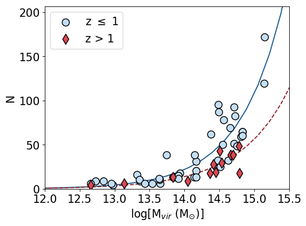
Figure 11: Exponential function fits relating the known structures’ virial masses, $M_{vir}$, to their magnitude cut member numbers $N$. The solid blue line is Equation 4, fitting the $z\leq 1$ structures denoted in blue, and the dashed red line is Equation 5, fitting the $z>1$ structures denoted in red.

This function gives the number of members brighter than the $m_{AB}<24.5$ magnitude cutoff in each redshift domain that we simulate. When we generate our mock groups and clusters, all of the mock member galaxies have magnitudes that are brighter than the magnitude cutoff at $z$ = 0.8. However, this is not the case at $z$ = 1.2, where many of the galaxies that are generated are fainter than this limit. Thus, in order to match the number of mock members at $m_{AB}<24.5$ with the number of true members at $m_{AB}<24.5$ as estimated by Equation 5, we need to inject a larger number of members into the mocks to account for the eventual loss of fainter members. To determine the number of members that we must inject into our mock catalogs at a given structure mass at $z>1$, we first take the number of members predicted by Equation 5 and then correct that number by dividing by the fraction of members in $z>1$ mock clusters and groups that are brighter than the magnitude limit cutoff. This value is calculated to be 0.743 and 0.583 for cluster and groups, respectively, on average, meaning that, in the mocks at $z>1$, the $N_{mem}$ recoverd by Equation 5 must be multiplied by 1/0.743 and 1/0.583 for cluster and group members to generate the number mock members brighter than the magnitude cutoff that match the observations.

To further support our member galaxy numbers, we looked to the Millennium Run dark matter simulation embedded with the semianalytical model of De Lucia & Blaizot (2007) in order to try to account for the presence of poorly occupied halos that may be missing and were not included in our mocks. We took a snapshot at $z$ = 0.988 to compare with our $z\sim$1 population and selected all friend-of-friend clusters and groups with masses above $\log(M_{tot}/M_{\odot})>13.3$, where the friend-of-friend clusters and groups were taken from the simulation output. Fig. 12 shows the median number of galaxies in these friend-of-friend clusters in each 0.2 dex halo mass bin. For a given halo mass and a given tracer population (i.e., the stellar mass bin), we see that the interquartile range encompasses a relatively small range in $N_{gals}$, with the largest variations reaching $\sim$20%. In addition, the numbers of galaxies appear to be broadly consistent with the numbers presented in Fig. 11 and estimated by Equations 4 and 5 for stellar masses larger than $\log(M_{tot}/M_{\odot})>10.0$ to $10.5$, which is represenative of our $z\sim$1 population. This shows that poorly occupied halos do not significantly impact the numbers of member galaxies estimated, which lends credulity to the purity and completeness estimates we will find with the mocks later on.

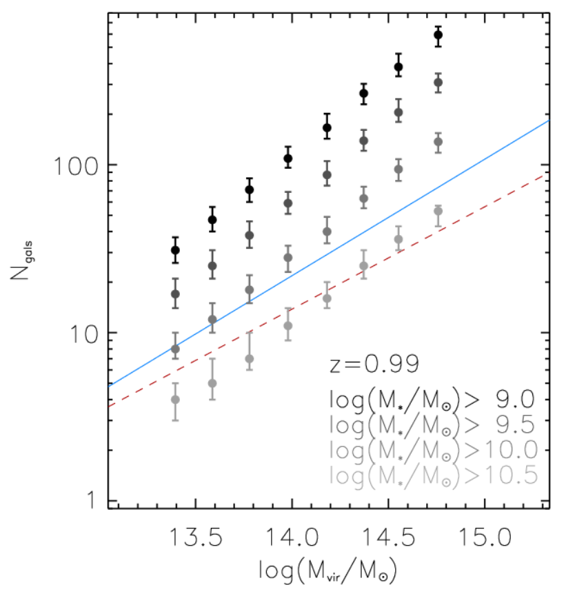
Figure 12: We selected all friend-of-friend clusters and groups with masses above $\log(M_{tot}/M_{\odot})>13.3$ in the Millennium Run dark matter simulation embedded with the semianalytical model of De Lucia & Blaizot (2007) at $z$ = 0.988. Plotted is the median number of galaxies in these friend-of-friend clusters, in bins of 0.2 dex in total friend-of-friend mass. Each of the four series of points contains galaxies with stellar mass $SM$ larger than the given threshold in the labels. Error bars on the median values represent the 25th and 75th percentile of the counts distribution in each bin. The interquartile range encompasses a relatively small range in $N_{gals}$ for each given halo mass and stellar mass bin, with the largest variations reaching $\sim$20%. The numbers of galaxies for the larger stellar mass bins are also broadly consistent with the numbers presented in Fig. 11 and estimated by Equations 4 and 5.

5.1.4 Injecting Structures in the Mock Catalogs

We create our mocks such that we have a total of 300 clusters and 300 groups at each redshift. We defined our mock clusters to have velocity dispersions between 580 and 1100 km s^-1, the upper bound matching the largest known structures in the ORELSE fields. Mock groups were defined as having velocity dispersions of 300 and 500 km s^-1. For each new mock generated, we used uniform random sampling of the velocity dispersions for all injected mock groups and clusters. Virial masses of each mock cluster or group are calculated directly from the imposed velocity dispersion and systemic redshift. Ignoring the uncertainty values in the fit of $M_{vir}$ versus $N_{mem}$, this corresponded to 35 to 131 members for clusters and between 9 and 25 members for groups at $z$ = 0.8. We then sample the appropriate Schechter function for the member galaxies to generate the magnitude distributions of each structure.

To test how well our detection algorithm performed when varying the velocity dispersion of the injected structures, we arranged the groups and clusters into two bins, cleanly separating their velocity dispersion ranges into lower and upper halves and effectively forming two mass bins. We injected our groups and clusters using two different arrangements for both the lower and upper mass bins. One arrangement is a single cluster and three groups and the other is two clusters alone. We stipulated our injected clusters to have their centers at least 4 Mpc apart, or 2 Mpc in the case of groups. This is done to avoid any spatial overlap between the injected structures. Such chance alignments of multiple structures in real data would lead to a higher probability of detecting a structure at their location, so our mocks cover the scenario in which detection is most difficult, meaning our purity and completeness numbers are necessarily lower limits.

For every mock at the same redshift, we used the exact same field galaxy distribution. We ran 50 mocks for each mass bin, making for a total of 150 groups and clusters for each mass bin at each of our tested redshifts. To test how well our detection algorithm performed at varying levels of spectroscopic coverage, we ran each mock through the Voronoi tessellation Monte-Carlo (VMC) four times, each at a different spectroscopic coverage level (5%, 20%, 50%, and 80%). Each time, we randomly assign that given fraction of all the galaxies in the mock spectral redshifts. We treat the remaining galaxies as only having $z_{phot}$ values. The catastrophic outlier rate is set to 6% to match the average seen in the ORELSE photometric catalogs. The photometric redshifts $pz$ are modified by the average $z_{phot}$ error $pz_{err}$ (set to 3% to match the average of the SC0849 and RXJ1716 fields) such that:

$$pz=pz+Rpz_{err}(1+pz)$$ (6)

where $R$ is a normalized Gaussian. This modification operates under the assumption that there is no change in $z_{phot}$ accuracy nor the catastrophic outlier rate as a function of magnitude to the depth of our mock data. $z_{phot}$ values that end up as catastrophic outliers are randomly set to redshifts of 0.31 and below. This reflects what we see in the real data, where the vast majority of $z_{phot}$ outliers are higher redshift galaxies that scatter to lower redshifts. After making a magnitude cut only keeping the galaxies brighter than 24.5, the VMC map is then made in the same manner as it was for the real ORELSE fields.

5.2 Assessing Purity and Completeness with the Mock Catalogs

We looked for detections in the mock VMC overdensity maps with the same parameters as in §4.3. In other words, we use DETECT_THRESH = 4$\sigma$, DETECT_MINAREA = 20 corresponding to a $\sim$0.1 Mpc² area, no smoothing filter, DEBLEND_NTHRESH = 32, DEBLEND_MINCONT = 0.01. As with the search of the real data, we discard detections in the mocks with $\sigma_{z}>0.05$ for being unphysically large, and we exclude detections where the Gaussian peak was more than 20% higher than the maximum flux of the fitted points to cut out detections with higher likelihoods of inaccurate total masses and redshifts. We also exclude the most poorly constrained detections by removing cases where the uncertainty on the integrated isophotal flux was larger than the integrated isophotal flux. This removal largely does not affect what we find for our purity and completeness values other than a small improvement to purity at high spectroscopic fractions. Recovered structures were identified by looking within a linking radius of 1 Mpc and a redshift window of $\Delta z$ = 0.02 for each injected structure’s position and redshift, which are the identical values used for the search on the real data.

We test whether we find the same optimal SExtractor parameters with the mocks as we did earlier with our tests on the real data. This serves as a self-consistency check and demonstrates whether the mocks are representative of the real data or not. We run SExtractor on the VMC overdensity maps of the mocks for 14 total pairs of parameters, varying the DETECT_THRESH between 4 and 5$\sigma$ and DETECT_MINAREA between 20, 30, 40, 50, 60, 70, and 80 square pixels. The absolute value of the DETECT_THRESH parameter is based on the background RMS averaged from the polynomial fits of the background RMS of all the fields in the real data. The final absolute DETECT_THRESH value is the resulting RMS value at the particular redshift multiplied by the DETECT_THRESH $\sigma$ used. We do not vary the choice of deblending parameters, as we injected structures such that they were separated by at least 2 Mpc, so any variation in the deblending is unlikely to change our results. The detection algorithm used on these mocks hereafter is the same as the procedure we used on the real data.

To assess the total purity and completeness values, we calculated the product of the purity and completeness numbers for all SExtractor parameter pairs across all spectroscopic coverage levels at both of our tested redshifts. The completeness is defined as only structures we recovered divided by the total number of structures we injected into the mocks. The purity is the fraction of all of our detections that we were able to match up to our injected structures. We calculate the mean purity and completeness for all mocks at each spectroscopic coverage level. We statistically quantify the uncertainties in the purity and completeness using a bootstrap method. We subsample each level of spectroscopic coverage by randomly taking 20 mocks and measuring their purity and completeness, repeating this process 1000 times. We then obtain a median purity and completeness value and their 1$\sigma$ uncertainties for a given level of spectroscopic coverage.

We found that there was no overall best performing set of SExtractor parameters, with each pair showing similar performance in both purity and completeness for each redshift (Fig. 13, Table 3). SExtractor was able to detect the regularly shaped structures in the mock catalogs regardless of how sensitive the detection thresholds we used were. We thus choose to use the 4$\sigma$ DETECT_THRESH and DETECT_MINAREA of 20 to maximize our chances of detecting an overdensity candidate, which are the same parameters we found to work best in our tests in §4.3. We additionally tested how our purity and completeness numbers were in the 0% spectroscopic fraction case, finding them to be very low, with completeness under $\sim$10% and purity at most around 50% for both redshifts. Our purity and completeness markedly improve for even 5% spectroscopic coverage, where our purity and completeness are, respectively, 96% and 57% for $z$ = 0.8, and 70% and 29% for $z$ = 1.2 for our choice of SExtractor parameters (Table 3). We thus choose to limit our search range to areas with spectroscopic coverage of at least 5% when applying our algorithm to the real data.

We also assessed how the product of the purity and completeness vary when using different-sized Gaussian filters in SExtractor, as well when using no filtering at all. We found there was at most a 5 to 10% improvement by applying some measure of filtering for our detection parameters of choice. We expect the best performance from filtering comes from recovering regularly shaped structures as we have injected into the mocks. This is not necessarily true for structures in the real data however. Since the changes were minor, we elected to use no filtering when running SExtractor on our real data so as to increase the chances of detecting all structures in our fields and to avoid biasing ourselves against detecting irregularly shaped structures.

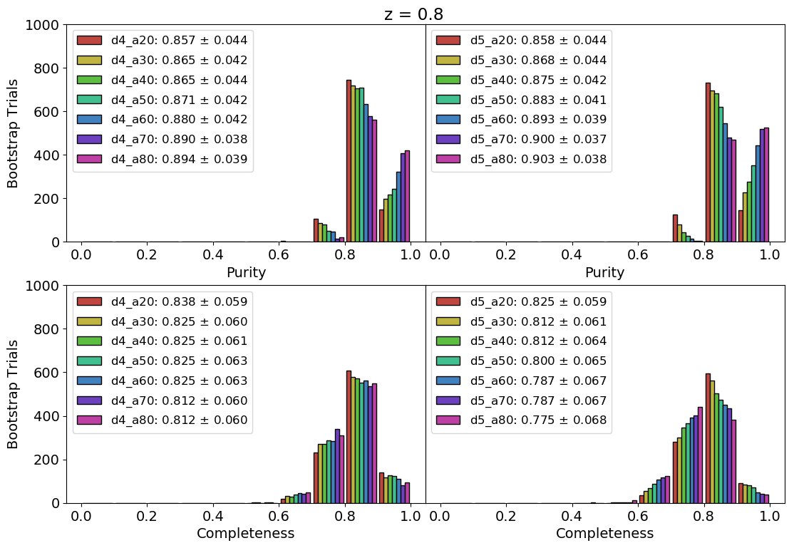
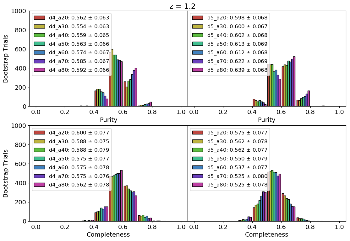
Figure 13: Depicted in this figure are the purity and completeness across all mocks over all spectroscopic coverage levels. To assess the uncertainties in the purity and completeness, we used a bootstrap method where we calculated the purity and completeness for a random 20 mocks which is then repeated 1000 times. We combined our purity and completeness bootstrap routines to compute the purity and completeness values for each SExtractor parameter pair of DETECT_THRESH of 4 and 5$\sigma$ and DETECT_MINAREA of 20, 30, 40, 50, 60, 70, and 80 square pixels for $z=0.8$ and $z=1.2$. The DETECT_MINAREA parameters are denoted by the color of each bar in the histogram, with the 4 and 5$\sigma$ DETECT_THRESH parameters spilt into the left and right panels. The mean purity and completeness and their 1$\sigma$ uncertainties for each pair is given in the legends. The uncertainties in the purity and completeness values show little dependence on the choice of SExtractor parameters.

Table 3: Purity and Completeness for Different SExtractor Parameters

Redshift	DETECT_THRESH	DETECT_MINAREA	5% $z_{spec}$	20% $z_{spec}$	50% $z_{spec}$	80% $z_{spec}$
0.8	4	20	P/C = 0.959/0.573	P/C = 0.926/0.826	P/C = 0.797/0.940	P/C = 0.755/0.973
			P$\cdot$C = 0.550	P$\cdot$C = 0.765	P$\cdot$C = 0.750	P$\cdot$C = 0.735
0.8	4	30	P/C = 0.961/0.568	P/C = 0.930/0.823	P/C = 0.800/0.938	P/C = 0.764/0.973
			P$\cdot$C = 0.546	P$\cdot$C = 0.765	P$\cdot$C = 0.750	P$\cdot$C = 0.743
0.8	4	40	P/C = 0.965/0.569	P/C = 0.933/0.818	P/C = 0.803/0.938	P/C = 0.771/0.971
			P$\cdot$C = 0.549	P$\cdot$C = 0.763	P$\cdot$C = 0.753	P$\cdot$C = 0.749
0.8	4	50	P/C = 0.968/0.562	P/C = 0.935/0.815	P/C = 0.811/0.935	P/C = 0.782/0.970
			P$\cdot$C = 0.544	P$\cdot$C = 0.762	P$\cdot$C = 0.758	P$\cdot$C = 0.759
0.8	4	60	P/C = 0.968/0.566	P/C = 0.935/0.809	P/C = 0.821/0.932	P/C = 0.798/0.968
			P$\cdot$C = 0.548	P$\cdot$C = 0.756	P$\cdot$C = 0.765	P$\cdot$C = 0.772
0.8	4	70	P/C = 0.970/0.565	P/C = 0.939/0.805	P/C = 0.840/0.924	P/C = 0.807/0.961
			P$\cdot$C = 0.548	P$\cdot$C = 0.759	P$\cdot$C = 0.776	P$\cdot$C = 0.776
0.8	4	80	P/C = 0.973/0.562	P/C = 0.943/0.805	P/C = 0.846/0.920	P/C = 0.816/0.959
			P$\cdot$C = 0.547	P$\cdot$C = 0.759	P$\cdot$C = 0.778	P$\cdot$C = 0.783
0.8	5	20	P/C = 0.983/0.565	P/C = 0.940/0.811	P/C = 0.799/0.924	P/C = 0.716/0.976
			P$\cdot$C = 0.555	P$\cdot$C = 0.762	P$\cdot$C = 0.738	P$\cdot$C = 0.699
0.8	5	30	P/C = 0.981/0.561	P/C = 0.941/0.797	P/C = 0.809/0.920	P/C = 0.734/0.975
			P$\cdot$C = 0.550	P$\cdot$C = 0.750	P$\cdot$C = 0.744	P$\cdot$C = 0.716
0.8	5	40	P/C = 0.978/0.551	P/C = 0.941/0.785	P/C = 0.834/0.919	P/C = 0.751/0.974
			P$\cdot$C = 0.539	P$\cdot$C = 0.739	P$\cdot$C = 0.766	P$\cdot$C = 0.731
0.8	5	50	P/C = 0.978/0.540	P/C = 0.944/0.781	P/C = 0.843/0.911	P/C = 0.772/0.969
			P$\cdot$C = 0.528	P$\cdot$C = 0.737	P$\cdot$C = 0.768	P$\cdot$C = 0.748
0.8	5	60	P/C = 0.979/0.531	P/C = 0.944/0.779	P/C = 0.848/0.901	P/C = 0.796/0.963
			P$\cdot$C = 0.520	P$\cdot$C = 0.735	P$\cdot$C = 0.764	P$\cdot$C = 0.767
0.8	5	70	P/C = 0.979/0.529	P/C = 0.951/0.777	P/C = 0.861/0.892	P/C = 0.815/0.956
			P$\cdot$C = 0.518	P$\cdot$C = 0.739	P$\cdot$C = 0.768	P$\cdot$C = 0.779
0.8	5	80	P/C = 0.978/0.521	P/C = 0.953/0.766	P/C = 0.869/0.882	P/C = 0.824/0.948
			P$\cdot$C = 0.510	P$\cdot$C = 0.730	P$\cdot$C = 0.766	P$\cdot$C = 0.781
1.2	4	20	P/C = 0.698/0.286	P/C = 0.602/0.485	P/C = 0.516/0.746	P/C = 0.433/0.858
			P$\cdot$C = 0.200	P$\cdot$C = 0.292	P$\cdot$C = 0.385	P$\cdot$C = 0.372
1.2	4	30	P/C = 0.694/0.285	P/C = 0.598/0.472	P/C = 0.514/0.738	P/C = 0.440/0.861
			P$\cdot$C = 0.198	P$\cdot$C = 0.282	P$\cdot$C = 0.379	P$\cdot$C = 0.379
1.2	4	40	P/C = 0.701/0.280	P/C = 0.608/0.471	P/C = 0.515/0.734	P/C = 0.447/0.861
			P$\cdot$C = 0.196	P$\cdot$C = 0.286	P$\cdot$C = 0.378	P$\cdot$C = 0.385
1.2	4	50	P/C = 0.712/0.276	P/C = 0.603/0.466	P/C = 0.517/0.730	P/C = 0.463/0.851
			P$\cdot$C = 0.197	P$\cdot$C = 0.281	P$\cdot$C = 0.377	P$\cdot$C = 0.394
1.2	4	60	P/C = 0.727/0.274	P/C = 0.618/0.464	P/C = 0.523/0.729	P/C = 0.478/0.845
			P$\cdot$C = 0.199	P$\cdot$C = 0.287	P$\cdot$C = 0.381	P$\cdot$C = 0.404
1.2	4	70	P/C = 0.725/0.268	P/C = 0.626/0.458	P/C = 0.530/0.728	P/C = 0.495/0.843
			P$\cdot$C = 0.194	P$\cdot$C = 0.287	P$\cdot$C = 0.386	P$\cdot$C = 0.417
1.2	4	80	P/C = 0.733/0.266	P/C = 0.627/0.454	P/C = 0.539/0.719	P/C = 0.515/0.835
			P$\cdot$C = 0.195	P$\cdot$C = 0.285	P$\cdot$C = 0.388	P$\cdot$C = 0.430
1.2	5	20	P/C = 0.747/0.228	P/C = 0.667/0.477	P/C = 0.542/0.706	P/C = 0.491/0.873
			P$\cdot$C = 0.170	P$\cdot$C = 0.318	P$\cdot$C = 0.383	P$\cdot$C = 0.429
1.2	5	30	P/C = 0.757/0.223	P/C = 0.675/0.470	P/C = 0.538/0.694	P/C = 0.505/0.868
			P$\cdot$C = 0.169	P$\cdot$C = 0.317	P$\cdot$C = 0.373	P$\cdot$C = 0.438
1.2	5	40	P/C = 0.755/0.220	P/C = 0.683/0.459	P/C = 0.538/0.686	P/C = 0.511/0.858
			P$\cdot$C = 0.166	P$\cdot$C = 0.313	P$\cdot$C = 0.369	P$\cdot$C = 0.438
1.2	5	50	P/C = 0.755/0.211	P/C = 0.679/0.450	P/C = 0.544/0.682	P/C = 0.532/0.849
			P$\cdot$C = 0.159	P$\cdot$C = 0.306	P$\cdot$C = 0.371	P$\cdot$C = 0.452
1.2	5	60	P/C = 0.753/0.206	P/C = 0.678/0.443	P/C = 0.553/0.672	P/C = 0.541/0.820
			P$\cdot$C = 0.155	P$\cdot$C = 0.300	P$\cdot$C = 0.372	P$\cdot$C = 0.444
1.2	5	70	P/C = 0.755/0.198	P/C = 0.680/0.432	P/C = 0.571/0.666	P/C = 0.552/0.814
			P$\cdot$C = 0.149	P$\cdot$C = 0.294	P$\cdot$C = 0.380	P$\cdot$C = 0.449
1.2	5	80	P/C = 0.761/0.193	P/C = 0.680/0.429	P/C = 0.591/0.649	P/C = 0.580/0.806
			P$\cdot$C = 0.147	P$\cdot$C = 0.292	P$\cdot$C = 0.384	P$\cdot$C = 0.467

Purity and completeness values for each set of SExtractor parameters we tested separated by spectroscopic coverage and redshift. There is not a strong dependence on the choice of SExtractor parameters, but we chose to use the most lenient set of parameters: DETECT_THRESH = 4$\sigma$ and DETECT_MINAREA = 20, to maximize our chances of detecting an overdensity candidate in the real data, which may not be regular in shape and thus more difficult to detect.

6 Final Overdensity Candidate Catalog

We conducted our overdensity candidate search over a total of 15 ORELSE fields with similar depth $B$- and $V$-band imaging as well as $riz$ and some form of ground- and/or space-based NIR imaging. We typically had an average of 11 bands per field (see §2 and Table 13 for details regarding the imaging and depth for each field). We searched for overdensity candidates with the same SExtractor parameters we found to work best overall in Sections 4.3 and 5: DETECT_THRESH = 4$\sigma$, DETECT_MINAREA = 20, DEBLEND_NTHRESH = 32, and DEBLEND_MINCONT = 0.01. We restricted our search to overdensity candidates with mean redshifts within our total redshift range, $z$ = 0.55 to 1.37. To reduce the chance of detecting the same overdensity more than once, we looked at the largest peaks in each field and excluded detections within 0.7 Mpc and $\Delta z<$ 0.02 of those peaks, as mentioned in §3.2.1.

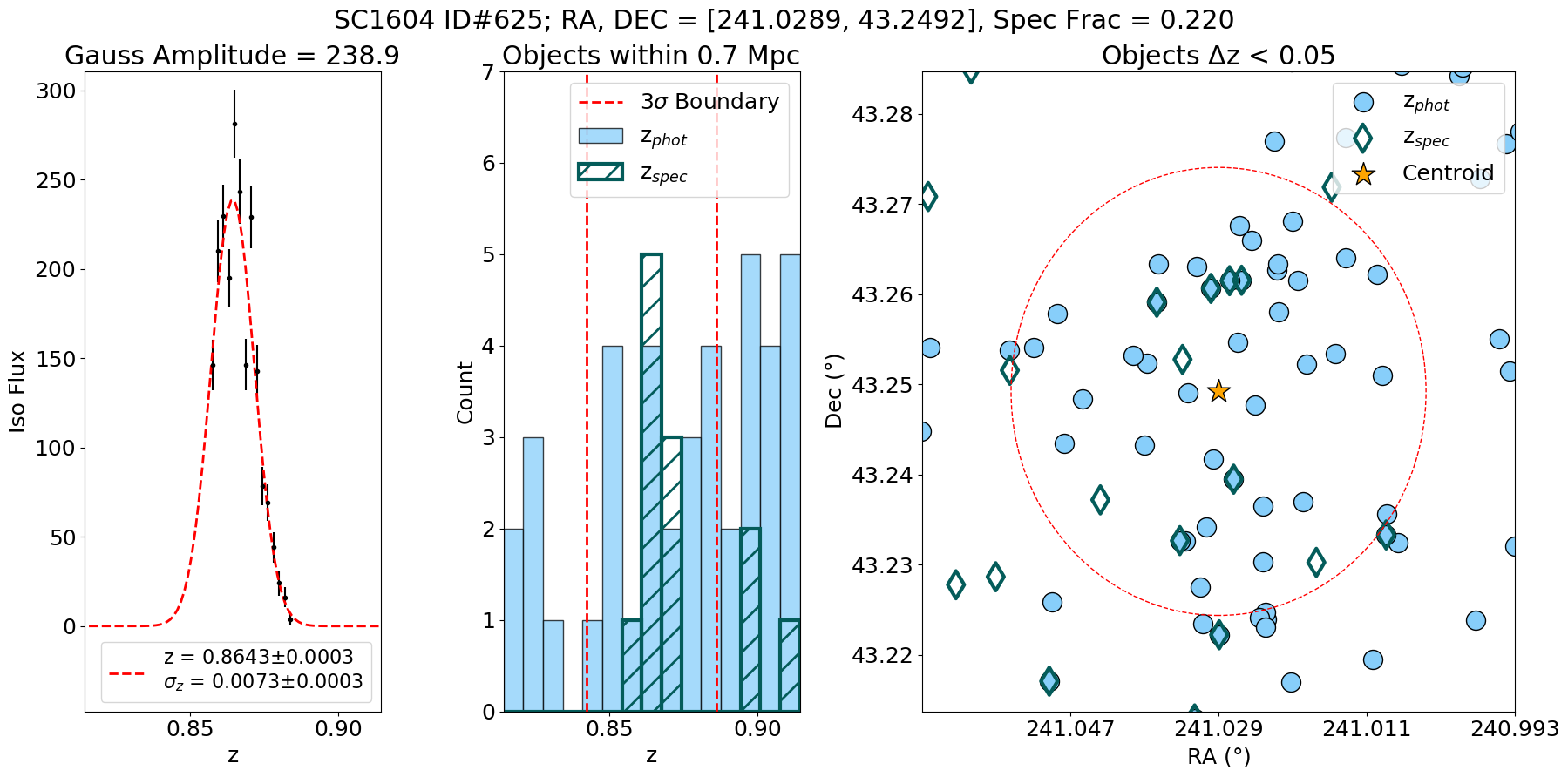
Figure 15: One example of a detected overdensity candidate. The left panel shows the overdensity candidate’s isophotal flux profile fitted with a Gaussian. The points in the profile come from linking individual isophotal detections in neighboring redshift slices whose flux-weighted distances were within a 1 Mpc linking radius. The associated errors in the isophotal flux is calculated by SExtractor. The center panel shows the histogram of spectroscopic and photometric members within a 0.7 Mpc radius from the centroided position of the overdensity candidate. The red dashed lines show the redshift boundary within 3$\sigma$ as determined by the Gaussian fit. The right panel plots the positions of the galaxy members within $\Delta z<0.05$ in a square measuring 1 Mpc on a side, and the dashed red circle has a radius of 0.7 Mpc.

We considered known structures identified if a detection was made within 1 Mpc of their fiducial transverse position and $\Delta z<$ 0.02 of their fiducial redshift. We discard overdensity candidates with $\sigma_{z}>0.05$ for being unphysically large. We also exclude candidates where the Gaussian peak was more than 20% higher than the maximum flux of the fitted points as well as candidates with larger integrated isophotal flux uncertainties than integrated isophotal fluxes, which were more likely to have inaccurate total masses and redshifts. Due to the purity and completeness numbers we saw with our tests with using reduced spectroscopic fractions in the mock catalogs in §5.2, we only included overdensity candidates in the final catalog with at least 5% spectroscopic fractions (see later on in this section for the meaning of the spectroscopic fraction in this context). After making this cut, our sample contained 51 of the 56 previously known clusters or groups (Table 4) and 402 new overdensity candidates (Table 5, Fig. 15, Fig. 18).

Table 4: Previously Known ORELSE Clusters and Groups

Name	Redshift	RA (J2000)	Dec (J2000)	$\sigma$a	Nb	log(Mvir)c	Recovered?
SC1604 Lz	0.5995	241.03282	43.2057	771.9 $\pm$ 110.0	21	14.711 $\pm$ 0.186	Yes
SC1604 A	0.8984	241.09311	43.0821	722.4 $\pm$ 134.5	35	14.551 $\pm$ 0.243	Yes
SC1604 B	0.8648	241.10796	43.2397	818.4 $\pm$ 74.2	49	14.722 $\pm$ 0.118	Yes
SC1604 C	0.9344	241.03142	43.2679	453.5 $\pm$ 39.6	32	13.935 $\pm$ 0.114	Yes
SC1604 D	0.9227	241.14094	43.3539	688.2 $\pm$ 88.1	70	14.481 $\pm$ 0.167	Yes
SC1604 F	0.9331	241.20104	43.3684	541.9 $\pm$ 110.0	20	14.168 $\pm$ 0.265	Yes
SC1604 G	0.9019	240.92745	43.4030	539.3 $\pm$ 124.0	18	14.169 $\pm$ 0.300	Yes
SC1604 H	0.8528	240.89890	43.3669	287.0 $\pm$ 68.3	10	13.359 $\pm$ 0.310	Yes
SC1604 I	0.9024	240.79746	43.3915	333.0 $\pm$ 129.4	7	13.541 $\pm$ 0.506	Yes
SC1604 Hz	1.1815	241.07967	43.3215	661.5 $\pm$ 80.2	15	14.367 $\pm$ 0.158	Yes
SC1324 A	0.7566	201.20129	30.1924	873.4 $\pm$ 110.8	43	14.833 $\pm$ 0.165	Yes
SC1324 B	0.6971	201.08815	30.2158	677.1 $\pm$ 143.6	13	14.516 $\pm$ 0.276	Yes
SC1324 C	0.7574	201.25533	30.4158	353.0 $\pm$ 182.4	6	13.652 $\pm$ 0.673	Yes
SC1324 D	0.7382	201.00773	30.4164	205.9 $\pm$ 90.1	8	12.955 $\pm$ 0.579	Yes
SC1324 G	0.6759	201.18736	30.7995	186.3 $\pm$ 38.8	10	12.840 $\pm$ 0.271	Yes
SC1324 H	0.6990	201.22040	30.8408	346.4 $\pm$ 109.8	19	13.708 $\pm$ 0.393	Yes
SC1324 I	0.6956	201.20550	30.9665	847.1 $\pm$ 96.4	35	14.808 $\pm$ 0.148	Yes
SC1324 Hz	1.0979	201.18372	30.8228	509.3 $\pm$ 220.4	11	14.047 $\pm$ 0.564	Yes
XLSS005	1.0559	36.773036	-4.2972476	735.8 $\pm$ 108.2	19	14.536 $\pm$ 0.191	Yes
SG0023 A	0.8396	6.02560	4.3590	412.8 $\pm$ 119.2	14	13.836 $\pm$ 0.376	Yes
SG0023 B1	0.8290	5.97570	4.3884	176.3 $\pm$ 29.6	23	12.730 $\pm$ 0.219	Yes
SG0023 B2	0.8453	5.96970	4.3820	277.8 $\pm$ 41.0	38	13.319 $\pm$ 0.192	Yes
SG0023 C	0.8466	5.92470	4.3807	385.3 $\pm$ 54.3	45	13.744 $\pm$ 0.184	No*
SG0023 M	0.8472	5.96740	4.3199	418.8 $\pm$ 68.9	14	13.853 $\pm$ 0.214	Yes
SG0023 Hz	0.9799	5.99464	4.3570	218.2 $\pm$ 62.6	9	12.970 $\pm$ 0.374	Yes
RXJ1757	0.6931	269.33196	66.525991	862.3 $\pm$ 107.9	34	14.832 $\pm$ 0.250	Yes
RXJ1757 Hz	0.9456	269.20697	66.593766	290.5 $\pm$ 92.6	8	13.352 $\pm$ 0.415	Yes
RXJ1821	0.8168	275.38451	68.465768	1119.6 $\pm$ 99.6	52	15.142 $\pm$ 0.116	Yes
RXJ1821 Hz	0.9189	275.24066	68.437054	684.8 $\pm$ 97.4	19	14.476 $\pm$ 0.185	Yes
SC0910 LzA	0.7600	137.68681	54.3436	524.0 $\pm$ 159.4	11	14.166 $\pm$ 0.396	No
SC0910 LzB	0.7859	137.60865	54.3897	165.5 $\pm$ 30.5	10	12.658 $\pm$ 0.240	No
SC0910 A	1.1034	137.51280	54.3099	840.4 $\pm$ 244.0	23	14.698 $\pm$ 0.378	Yes
SC0910 B	1.1007	137.68489	54.3725	724.7 $\pm$ 151.4	25	14.506 $\pm$ 0.272	Yes
Cl1429	0.9871	217.28141	42.6826	911.1 $\pm$ 84.2	38	14.831 $\pm$ 0.185	Yes
Cl1137	0.9553	174.39786	30.008930	534.6 $\pm$ 81.1	28	14.144 $\pm$ 0.197	Yes
RXJ1053	1.1285	163.43097	57.591476	898.0 $\pm$ 142.0	28	14.778 $\pm$ 0.206	Yes
RXJ1053 Hz	1.2049	163.20387	57.584000	916.3 $\pm$ 194.8	11	14.786 $\pm$ 0.277	Yes
RXJ1221 A	0.7017	185.53798	49.2329	426.6 $\pm$ 71.3	18	13.923 $\pm$ 0.218	Yes
RXJ1221 B	0.7000	185.34103	49.3138	753.2 $\pm$ 122.5	36	14.654 $\pm$ 0.222	Yes
RXJ1716 A	0.8158	259.10074	67.085108	624.1 $\pm$ 136.1	40	14.380 $\pm$ 0.284	Yes
RXJ1716 B	0.8092	259.21686	67.139647	1120.6 $\pm$ 101.5	83	15.145 $\pm$ 0.118	Yes
RXJ1716 C	0.8146	259.25725	67.152497	678.4 $\pm$ 57.8	39	14.489 $\pm$ 0.111	No
RXJ1716 Hz	0.8531	259.30007	67.183591	757.4 $\pm$ 99.2	16	14.623 $\pm$ 0.171	Yes
Cl1350 A	0.8012	207.88457	60.0371	351.2 $\pm$ 92.4	9	13.802 $\pm$ 0.343	Yes
Cl1350 B	0.8017	207.53970	60.1034	300.0 $\pm$ 118.5	10	13.429 $\pm$ 0.515	Yes
Cl1350 C	0.7996	207.71545	60.1148	802.4 $\pm$ 83.9	43	14.712 $\pm$ 0.149	Yes
RCS0224 A	0.7780	36.15714	-0.0949	825.4 $\pm$ 193.2	34	14.754 $\pm$ 0.305	Yes
RCS0224 B	0.7781	36.14123	-0.0394	710.7 $\pm$ 58.8	52	14.559 $\pm$ 0.108	Yes
RCS0224 Hz	0.8454	36.32021	-0.0928	437.7 $\pm$ 115.8	15	13.911 $\pm$ 0.345	Yes
SC0849 A	1.2637	132.23463	44.761780	714.4 $\pm$ 171.6	13	14.448 $\pm$ 0.313	Yes
SC0849 B	1.2639	132.29977	44.865903	261.5 $\pm$ 62.6	12	13.139 $\pm$ 0.312	Yes
SC0849 C	1.2609	132.24443	44.866012	839.2 $\pm$ 111.8	25	14.659 $\pm$ 0.174	Yes
SC0849 D	1.2703	132.14184	44.896338	697.2 $\pm$ 111.2	23	14.415 $\pm$ 0.208	Yes
SC0849 E	1.2601	132.27496	44.959253	445.1 $\pm$ 71.9	14	13.833 $\pm$ 0.210	Yes
SC0849 LzB	0.5678	132.24487	44.896184	495.2 $\pm$ 169.3	8	14.140 $\pm$ 0.445	No
SC0849 LzA	1.1394	132.28743	44.855804	176.3 $\pm$ 107.1	6	12.655 $\pm$ 0.791	Yes

$a$: 1 Mpc velocity dispersion in km s^-1, determined with a biweight estimator.

$b$: Number of galaxies used for the velocity dispersion calculation.

$c$: Virial mass in units of solar mass, calculated from the formula given in Lemaux et al. (2012).

All 56 previously known clusters and groups in the 15 ORELSE fields we conducted our search over, of which we recovered 51 with our VMC overdensity detection method. RA and Dec centers were calculated from an $i$-band weighted mean of galaxies within 1 Mpc (or $z$-band for redshifts greater than 0.95). Because of how we cut out detections within 0.7 Mpc of more significant peaks, we miss the detection of SG0023 C as we find it within 0.38 Mpc of the larger SG0023 B2 detection. Dropping the separation threshold to include SG0023 C however results in more duplicate detections of other known structures and thus likely more duplicate detections of the overdensity candidates. We thus decide that the 0.7 Mpc separation is more appropriate for the general use case here.

For one of the known structures that was not detected, SG0023 C, our minimum separation threshold of 0.7 Mpc between detections results in it being dropped from the detected sample as its detection is within 0.38 Mpc of where we find the more significant SG0023 B2 detection. If we were to drop the separation threshold so as to include SG0023 C, we find 14 total duplicate detections of other known structures, whereas keeping the 0.7 Mpc separation only results in 5 duplicate detections. As the supercluster in SG0023 is an especially difficult to separate system, we elect to use the 0.7 Mpc separation for its advantages in the more general case scenario and reduce our probability of having duplicate detections of the same overdensity candidates.

We checked sub-samples of the recovered known structures based on their spectroscopic fraction, mass, and isolation from other structures. We calculated the redshift offsets between what we find with our Gaussian fits and the fiducial values, as well as the median absolute deviation of these offsets. The variations in the median redshift offset and absolute deviations were tens of thousandths at most, or $<$100 km s^-1 at these redshifts, for each sub-sample, showing strong promise for our ability to find structures even at small spectroscopic fractions and low masses (Fig. 14).

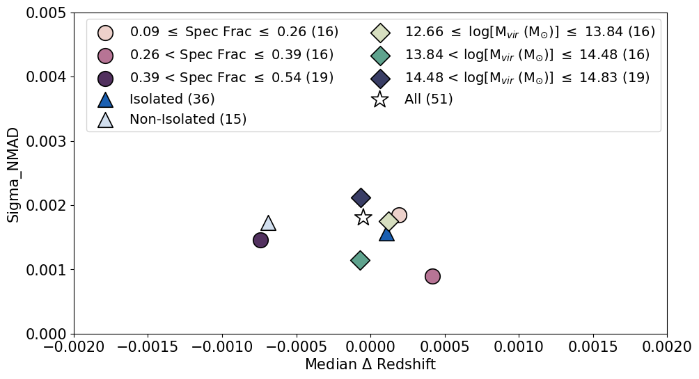
Figure 14: Median redshift offsets and their median absolute deviations for all recovered known structures between what was found with our Gaussian fits and the fiducial values. These were additionally binned into three sets of sub-samples based on their spectroscopic fraction, mass, and whether they were isolated from other structures or not. In each case, the differences between the bins were minor, and the absolute scale on both axes is on the order of tens of thousandths at most or $<$100 km s^-1 at these redshifts.

We approximate the spectroscopic fraction of an overdensity candidate by calculating the fraction of $z_{phot}$ galaxies within 0.7 Mpc of the overdensity candidate’s barycenter and $\Delta z<0.05$ of its redshift with a high-quality $z_{spec}$ counterpart. We use 0.7 Mpc as an average of the typical sizes of the known ORELSE groups and clusters. Because the redshifts of $z_{phot}$ galaxies are more uncertain than $z_{spec}$ galaxies, they may be scattered in or out of a given redshift range. The true spectroscopic fraction $Q_{true}$ involves estimating the true number of $z_{phot}$ galaxies in the redshift range with the following:

$$N_{true}=N_{phot}\times\frac{P_{gal}}{C_{gal}}$$ (7)

$$P_{gal}=\frac{N_{conf,A}}{N_{conf,A}+N_{conf,out}}$$ (8)

$$C_{gal}=\frac{N_{conf,A}}{N_{conf,A}+N_{conf,B}}$$ (9)

$$Q_{true}=\frac{N_{conf,A}+N_{conf,B}}{N_{true}}$$ (10)

$P_{gal}$ and $C_{gal}$ are the purity and completeness for the member galaxies respectively. Note that these purity and completeness values have no relation to the calculated purity and completeness of the detections in the mocks. $N_{true}$ is the true number of galaxies in the redshift range. $N_{phot}$ is the number of $z_{phot}$ galaxies in the redshift range. $N_{conf,A}$ and $N_{conf,B}$ are the $z_{spec}$ galaxies in the redshift range with a match to a $z_{phot}$ galaxy with a match inside or outside the redshift range respectively. $N_{conf,out}$ are the $z_{phot}$ galaxies with a $z_{spec}$ match outside the redshift range. Mathematically, $Q_{true}$ simplifies to:

$$\begin{split}Q_{true}&=\frac{N_{conf,A}+N_{conf,B}}{N_{phot}}\frac{C}{P}\\ &=\frac{N_{conf,A}+N_{conf,B}}{N_{phot}}\frac{\frac{N_{conf,A}}{N_{conf,A}+N_{conf,B}}}{\frac{N_{conf,A}+N_{conf,out}}{N_{conf,A}}}\\ &=\frac{N_{conf,A}+N_{conf,out}}{N_{phot}}\end{split}$$ (11)

6.1 Estimation of the Total Masses of the Candidates

To convert the isophotal flux from SExtractor into a physically meaningful value, we devised a new method of estimation by fitting the integrated Gaussian isophotal flux of our isolated known structures to their virial mass, where as in Section 4.3, we define a structure as isolated if no other known structures with a redshift $\Delta z<0.02$ are within a radial distance of 2.5 Mpc. While we make some assumption on the dynamical state of the structures used to calibrate this mass estimate, we selected a large number of isolated structures for this calibration both to limit the possible dynamical perturbation of these structures by surrounding structure and to average over variation in dynamical states. Further, as we will show in §6.1.2, this new method of mass estimation correlates extremely well with similar overdensity-based mass estimates meaning its accuracy has limited dependence on the type of structure or its galaxy population. Further, by virtue of the fact that virial mass estimates essentially match all other total mass measurements in ORELSE for those structures where independent mass measurements are available, our mass estimation also correlates well with X-ray, lensing, and Sunyaev-Zel’dovich masses of ORELSE structures.

We excluded four isolated structures from our fit: SC1604 Lz, SC1324 A, SC1324 I, and RXJ1053 Hz. SC1604 Lz is located near the redshift limit of our spectroscopic coverage. Its extended irregular structure and high mass additionally imply that it is not dynamically relaxed. SC1324 A and I are located at the most southern and northern edges of the field respectively and therefore partially off of the photometric footprint in that field. These structures in the VMC map are clipped by the edges of the image, and thus their integrated isophotal fluxes are artificially low. RXJ1053 Hz suffers from sparse sampling of its underlying velocity distribution and only has a small number of members.

We fitted four different models to the virial mass and integrated isophotal flux relation: a linear fit, a quadratic fit, an exponential fit, and a pseudo-Schechter function fit of the form log(M_vir) = $a+bF^{c}e^{-(F/d)}$, where M_vir is the virial mass in units of solar mass and F is the integrated isophotal flux. We find that there is a large scatter in masses at the low integrated isophotal flux end. To investigate this, we applied our fits to several different subgroups of our recovered isolated known structures cutting on their spectroscopic fractions (the top 75% or 50%) and number of members (requiring at least 10, 15, or 20 members). The spectroscopic fraction cuts were made on all recovered known structures, and the fits were applied to the isolated structures among them. Because the virial mass errors dominated, we only included them in the fitting and $\chi^{2}$ calculations, though the fits did not change meaningfully when we also included the integrated isophotal flux errors in the fitting process. We settled on using the pseudo-Schechter function fit from the isolated structures with the top 75% of spectroscopic fractions as it produced the smallest reduced $\chi^{2}$ of all the fits we attempted. We take the pseudo-Schechter model to use as our scaling relation between the integrated isophotal flux and virial mass with the parameters, $a$ = 15.691 $\pm$ 0.010, $b$ = -2.641 $\pm$ 0.033, $c$ = -0.327 $\pm$ 0.039, and $d$ = 124.174 $\pm$ 0.740, with an associated reduced $\chi^{2}$ of 0.263 (Fig. 16).

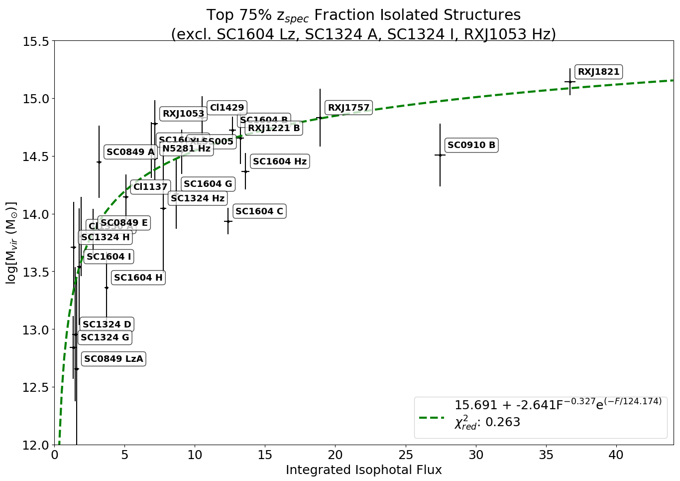
Figure 16: The integrated isophotal flux F of the Gaussian fits for selected isolated known structures, plotted against their virial masses. These structures were chosen based on removing the bottom 25% of all recovered known structures in spectroscopic fraction and selecting the isolated structures among the remaining. Four structures, SC1604 Lz, SC1324 A, SC1324 I, and RXJ1053 Hz, are treated as outliers in the fitting. In the fitting process, we only included the errors on the virial masses as they dominated over the errors on the integrated isophotal fluxes, though including both sets of errors did not meaningfully change the shapes of the fits. Of the four models we fitted for the virial mass, the pseudo-Schechter function had the smallest scatter and reduced $\chi^{2}$, where the terms are $a$ = 15.691 $\pm$ 0.010, $b$ = -2.641 $\pm$ 0.033, $c$ = -0.327 $\pm$ 0.039, and $d$ = 124.174 $\pm$ 0.740, with an associated reduced $\chi^{2}$ of 0.263.

6.1.1 Purity and Completeness by Mass

With a relation between mass and isophotal flux now in hand, we can calculate the purity and completeness numbers by mass bin in the mock catalogs. As a proxy for the “true” masses of all of the structures we injected into the mocks, we compute their virial masses based on their inputted virial radius, using Equation 2 in §4.3. When we compare these virial masses to the fitted masses based on their isophotal flux, we find the median difference between the two to be close to 0 for all spectroscopic fractions and both redshifts.

For the purity and completeness calculations, we divide the masses into four equal bins, which span from 13.2 $<\log(M/M_{\odot})<$ 15.0. We use the virial mass for the recovered injected structures and the fitted masses for the spurious detections. For each mass bin at each spectroscopic fraction at each redshift, we compute the purity and completeness through a bootstrap method, similar to the process in §5.2. We subsample and compute the purity and completeness of a random 20 detections, then repeat the process 1000 times (Fig. 17).

At low masses, it becomes difficult to separate overdensities that arise from real structure versus those that are nothing more than field fluctuations. In these cases, lower spectroscopic fractions which wash out small overdensities to the point of non-detection are more resistant to contamination by field fluctuations, and so we see lower purity numbers at higher spectroscopic fractions. However, we do not know if the low mass spurious detections are actually present in the field or not, as the galaxies are taken from real data, so we caution readers to treat the purity numbers as lower limits. As we only have purity and completeness estimates for masses above $\log(M/M_{\odot})=13.2$, the lower mass candidates we found must similarly be taken with a grain of salt.

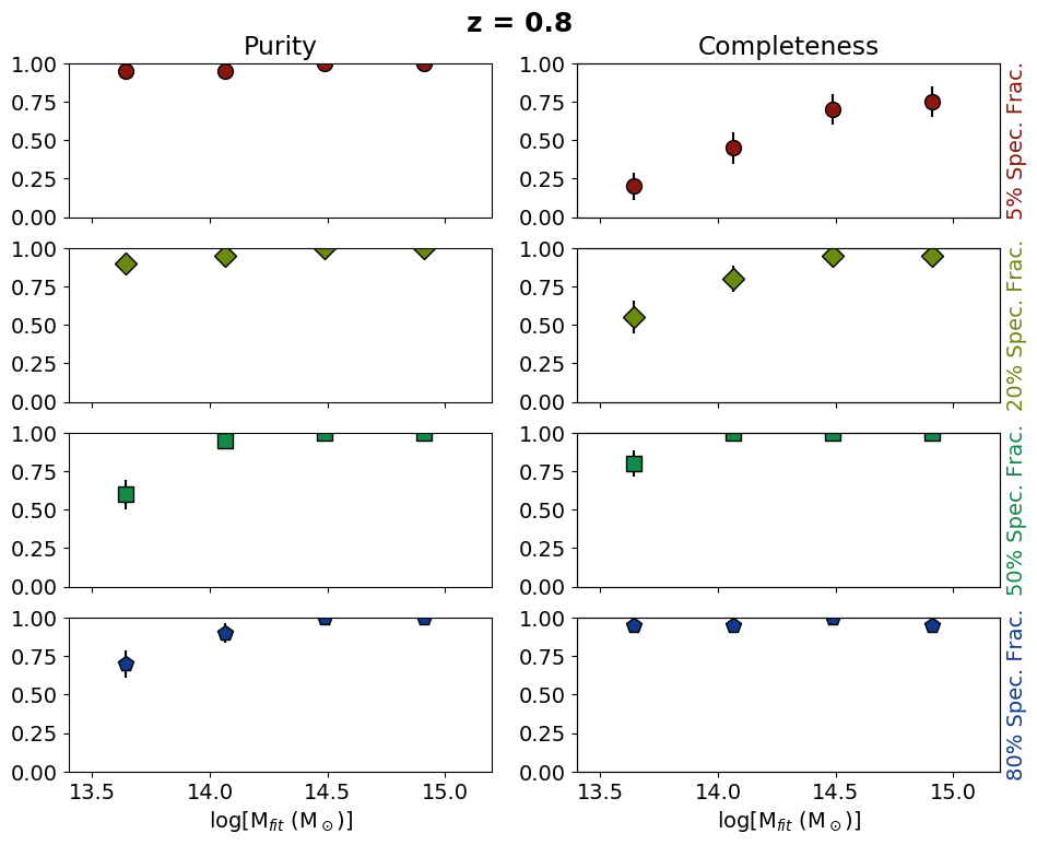
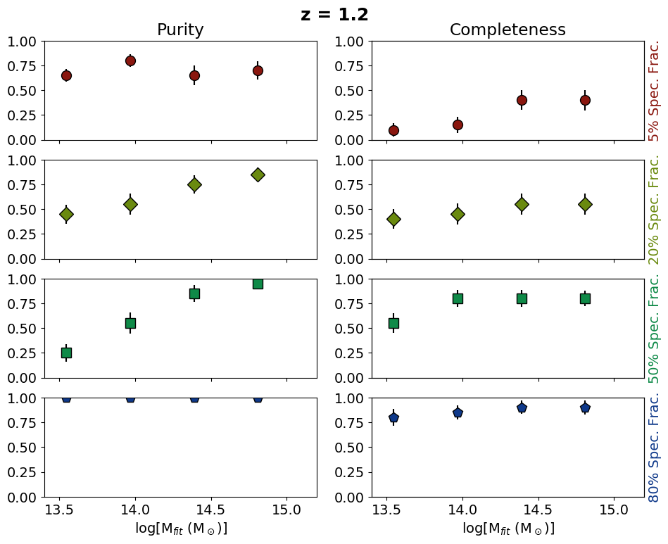
Figure 17: Purity and completeness numbers for the mock catalogs divided into four mass bins. The points plotted are the median values and their 1$\sigma$ uncertainty over 1000 bootstrap trials picking 20 random detections at a time. In some cases, the size of the marker was larger than the range of the error bar. Note that the mass bins are slightly different between the $z$ = 0.8 and $z$ = 1.2 plots due to small differences in the mass ranges for each redshift. We found that the purity tended to be higher at lower spectroscopic fractions, which is likely due to the many photometric objects washing out the small overdensities that arise from field fluctuations. It is possible these overdensities are real structure in the field, as we take the field from real data, so our purity numbers here are functionally lower limits.

6.1.2 Comparison with Overdensity Mass Estimation

As an additional check on our mass estimation, we compared our fitted mass estimation $M_{fit}$ to the method similar to the approach that is used in Cucciati et al. (2018). To make this comparison we first compiled the overdensity masses for the isolated structures which lay in the top half of all isolated structures in terms of spectral fraction, i.e., a similar population to that used in the fit described above. We then used the formalism of Cucciati et al. (2018) to measure the overdensity masses at a variety of different equivalent spherical radii by varying the isodensity threshold that defines the structure. The equivalent spherical radius is given as $(3/4*V)^{1/3}$, where $V$ is the volume of the isolated structure above a given density threshold. This overdensity mass was calculated at five different radii, running from $R_{vir}$ to $5R_{vir}$ in steps of one $R_{vir}$. At each step, the overdensity mass is calculated as $M_{tot}=\rho_{m}V(1+\delta_{m})$, where $\rho_{m}$ is the comoving matter density, $V$ is the volume of the isolated structure, and $\delta_{m}$ is the average matter overdensity within that volume. The average matter overdensity was calculated by the average $\delta_{gal}$ via $\delta_{m}=\delta_{gal}/b$, where $b$ is the bias factor of the galaxies comprising the overdensity measurement. While Cucciati et al. (2018) adopted a single bias factor, appropriate for their analysis at a single redshift, here we are required to adopt a bias factor that varies for each structure. This varying bias factor was estimated in the following manner. For the entire ORELSE spectroscopic sample subject to the criteria discussed in §2, we measured the median specific star-formation rate (SSFR) as a function of redshift as estimated by the FAST SED fitting described in Tomczak et al. (2017). The entire ORELSE sample was used instead of each individual field to smooth out any decrease in the average SSFR of galaxies caused by an individual structure (e.g., Tomczak et al., 2019). For an isolated structure at a given redshift, the average SSFR and the structure redshift was used to estimate $b$ from Coil et al. (2017). The adopted bias factor ranged from $b=1.12$ at $z=0.7$ to $b=1.27$ at $z=1.2$.

In order to determine the appropriate equivalent spherical radius for comparison to $M_{fit}$, we additionally calculated the elongation of each of the isolated structures at each step using the formalism of Cucciati et al. (2018). Briefly, elongation is defined as the average effective radius in the two transverse dimensions relative to the effective radius in the line-of-sight dimension. The effective radius is defined as $R_{e}=\sqrt{(\Sigma_{i}w_{i}(x_{i}-x_{peak})^{2}/\Sigma_{i}(w_{i}))}$, where $i$ is the $i_{th}$ pixel of the VMC map within the volume bounded by the structure along a given dimension, $w_{i}$ is the $\delta_{gal}$ value of that pixel, and $x_{i}$ is the location of the pixel relative to the barycenter location, $x_{peak}$, along the right ascension, declination, or redshift axes. Elongations, $E_{z/xy}$, were estimated in the range 6-30, with a mean value of $\langle E_{z/xy}\rangle=15.2$, i.e., at a given overdensity, the average isolated structure was 15.2$\times$ larger in the line-of-sight dimension than the transverse dimensions. Given the logic presented in §5.1.2, we choose the equivalent spherical radius that encompasses a volume similar to $4/3\pi$$1.5R_{vir}^{3}E_{z/xy}$, as this radius contains a large fraction of the true members of a system while minimizing interlopers. This equivalent spherical radius is $4R_{vir}$. Overdensity masses for each isolated structure were measured in volumes with equivalent spherical radii of $4R_{vir}$ and compared to $M_{fit}$. This comparison yielded a median offset of $\langle\tilde{\Delta}_{\log(M_{tot})-\log(M_{fit})}\rangle=-0.221$ and a $\sigma_{NMAD}=0.391$ over $\sim$2.5 orders of magnitude in structure masses ($12.7\la\log(M_{tot}/M_{\odot})\la 15.2$). We note here that these values do not change meaningfully if we adopt a slightly smaller or larger equivalent spherical radius. Given the large number of assumptions in each method, this level of concordance between the two mass estimates is impressive, and we conclude that the $M_{fit}$ values measured here are broadly consistent with the $M_{tot}$ methodology of Cucciati et al. (2018).

We also compare these $M_{tot}$ values with the $M_{vir}$ of each respective isolated structures. By design, since $M_{fit}$ is anchored to $M_{vir}$ and because we see a large degree of concordance between $M_{tot}$ and $M_{fit}$, these values should be broadly similar. We verify that expectation here, finding a median offset of $\langle\tilde{\Delta}_{M_{tot}-M_{vir}})\rangle=-0.220$ and a $\sigma_{NMAD}=0.155$ again over $\sim$2.5 orders of magnitude in structure masses ($12.7\la\log(M_{tot}/M_{\odot})\la 15.2$). Again, given the different assumptions associated with the two methods, disavowing knowledge of the previous comparison, the level of concordance is striking. Finally, from our tests with the mock catalogs, we recall that our purity and completeness tend to drop off at lower masses, especially at higher redshifts. Because of this, we make no attempt to push the analysis in this paper to structure masses lower than the minimum mass range probed by the mocks, or $\log(M_{tot}/M_{\odot})\sim 13.5$.

7 Conclusions

Searching for galaxy overdensities is challenging, and many established methods depend on using assumptions on their shapes and other physical properties to detect them. In this work, we have presented a powerful new technique, Voronoi tessellation Monte-Carlo (VMC) mapping, and applied it to the rich ORELSE data set cut at 18 mag $\leq i/z\leq$ 24.5 mag (the equivalent of $10^{9}-10^{10}M_{\odot}$ stellar mass-limited sample), recovering 51 of the 56 known structures and finding 402 new overdensity candidates. Though we’ve applied the VMC method to one particular data set in this work, it can similarly be used for any photometric and spectroscopic data set.

How many overdensities the VMC method will find is tied heavily to the choice of its various parameters related to the mapping and detection, all of which we extensively tested to find what gave the best performance overall. We tested how varying the Source Extractor (SExtractor) detection parameters, DETECT_THRESH and DETECT_MINAREA, as well as the deblending parameters, DEBLEND_NTHRESH and DEBLEND_MINCONT, would affect how many known ORELSE structures we could recover. We also tested the SExtractor detection parameters on constructed mock catalogs with injected groups and clusters, where unlike with the real ORELSE data, we have the advantage of having full knowledge of what structures are present. From these tests, we concluded that the best parameters to use were DETECT_THRESH = 4$\sigma$, DETECT_MINAREA = 20, DEBLEND_NTHRESH = 32, and DEBLEND_MINCONT = 0.01. We also saw that the VMC method in its broad application can find many overdensities across a wide redshift range. However, it has some difficulty separating close or blended systems while avoiding splitting individual structures elsewhere. In this work, we elected to compromise on parameters that were not able to completely split systems like the superclusters in SG0023 or RXJ1716 as they performed best for all of the fields overall.

With the mock catalogs, we confirmed the best DETECT_THRESH and DETECT_MINAREA parameters we found with testing a subset of known structures by assessing our purity and completeness numbers across a range of simulated spectroscopic fractions. We found impressively high purity and completeness rates even at relatively small spectroscopic fractions, such as 0.92/0.83 and 0.60/0.49 for purity/completeness at $z=0.8$ and $z=1.2$ respectively for spectroscopic fractions of $\sim$20%.

Table 5 lists our 402 new overdensity candidates with their redshifts, transverse positions, fitted masses, and spectroscopic fractions. The total redshift range spanned by our candidates was 0.565 $<z<$ 1.371. We fixed the spectroscopic fraction floor to be no lower than 5%, and highest value was 76.9%. The estimated masses were between 10.2 $<\log(M_{fit}/M_{\odot})<$ 14.8 (Fig. 18). From purity and completeness tests with the mock catalogs, we found that the purity and completeness tend to be uniformly high at around $\log(M_{fit}/M_{\odot}\lower 2.15277pt\hbox{$\;\buildrel>\over{\sim}\;$}$ 14.5, especially at high spectroscopic coverage. We can also derive a total mass function from the overdensity candidates we detected, corrected using the purity and completeness numbers from the mocks and interpolated based on the three dimensions of redshift, mass, and spectroscopic coverage. We will be including such analysis in full in an upcoming paper. Note that we only have purity and completeness estimates for masses above $\log(M_{fit}/M_{\odot})=13.2$, so the lower mass candidates we find here must be taken with a grain of salt. However, we wished to include everything the algorithm found, and these low mass candidates make for good follow-up targets for confirmation in future work. Access to the code and maps we used in this work is also available upon request.

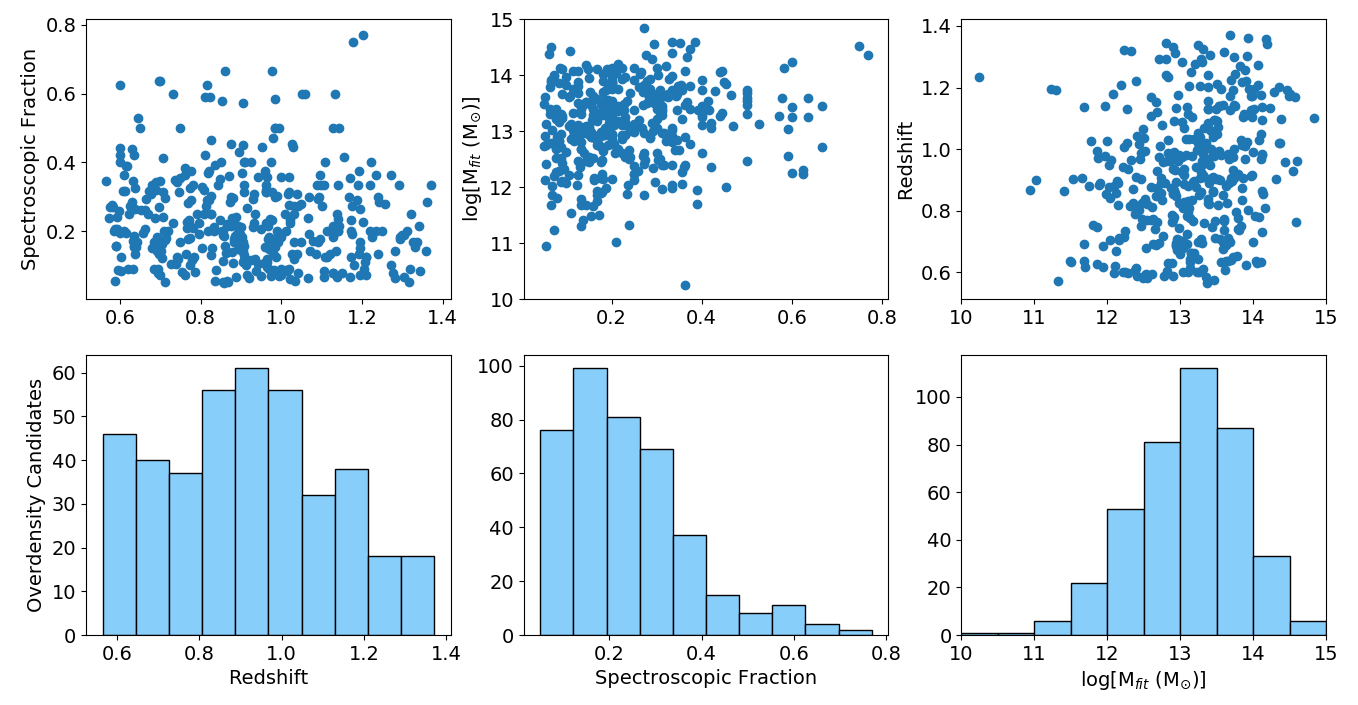
Figure 18: Scatter plots (top) and histograms (bottom) of the redshifts, spectroscopic fractions, and masses of the 402 new overdensity candidates listed in Table 5. The same x-axis is shared between the top and bottom panels for each column. The redshift range spanned between 0.565 $<z<$ 1.371. We set the spectroscopic fraction floor at 5%, and it reached a maximum of 76.9%. The estimated masses were between 10.2 $<\log(M_{fit}/M_{\odot})<$ 14.8. Our sensitivity to low-mass overdensities as well as the total number of overdensities detected tend to decline with greater redshift, which is the same behavior we saw in our mock catalog tests.

With the ORELSE dataset, we have demonstrated the ability of the VMC method to measure precise systemic redshifts, provide an estimate of the total gravitating mass, and maintain high levels of purity and completeness for both groups and clusters at intermediate redshifts ($z\sim 1$) even in the case of only moderate levels of spectroscopy. These factors speak to the value of the VMC method in applications for both current and future imaging surveys that either contain or overlap with some spectroscopic component. One such survey that has already been undertaken is the VIMOS Ultra Deep Survey (VUDS; Le Fèvre et al., 2015), a spectroscopic redshift survey of $\sim$5000 faint galaxies at redshifts of $2<z\simeq$ 6 over 1 square degree of the sky in well-known extragalactic fields with deep, high-quality imaging. While the VMC method has already demonstrated the ability to detect several overdensities in VUDS (e.g., Cucciati et al., 2018; Lemaux et al., 2018), we are currently adapting the methods presented in this paper to perform a systematic search for forming groups, clusters, and superclusters within VUDS in the high-redshift Universe. However, this survey will eventually be eclipsed in size and in depth by ongoing or near-term future surveys, e.g., the Hyper Suprime-Cam Subaru Strategic Program with follow-up observations from the Prime Focus Spectrograph, as well as future surveys envisioned for the coming decade following the rise of thirty meter class telescopes, dedicated 10-$m$ class telescopes such as the Maunakea Spectroscopic Explorer, and the next generation of space observatories that will enable imaging and spectroscopic surveys across an incredible redshift baseline for large swaths of the sky. With regards to the redshift regime covered by this paper, the new Anglo-Australian Telescope (AAT) Deep Extragalactic VIsible Legacy Survey (DEVILS; Davies et al., 2018) is a spectroscopic campaign designed for high completeness that will help to overcome many of the issues with using photometric redshifts at $0.3<z<1.0$. The Wide Area VISTA Extra-galactic Survey-Deep (WAVES-Deep; Driver et al., 2016) is a 4MOST Consortium Design Reference Survey aiming to obtain roughly 1.2 million spectroscopic galaxy redshifts over a 100 square degree area at z$\sim$1. Tools such as the VMC method presented here and its variants will be powerful in utilizing these data most effectively to find overdensities of galaxies of differing types from the local universe to the very highest of redshifts.

Table 5: New Overdensity Candidates

Candidate ID	Pointsa	Redshift	$\sigma_{z}^{b}$	RA (J2000)	Dec (J2000)	log(Mfit)c	Spec. Fraction
SC1604 6	6	0.5727 $\pm$ 0.0014	0.0048 $\pm$ 0.0020	241.00285	43.35538	11.32${}^{+0.38}_{-0.58}$	0.238
SC1604 18	11	0.6014 $\pm$ 0.0004	0.0068 $\pm$ 0.0006	241.10267	43.13988	13.23${}^{+0.15}_{-0.14}$	0.194
SC1604 19	9	0.5998 $\pm$ 0.0005	0.0051 $\pm$ 0.0007	241.13713	43.37485	12.24${}^{+0.13}_{-0.12}$	0.625
SC1604 20	9	0.5988 $\pm$ 0.0006	0.0053 $\pm$ 0.0008	241.07052	43.36816	12.28${}^{+0.14}_{-0.14}$	0.259
SC1604 22	11	0.6013 $\pm$ 0.0002	0.0043 $\pm$ 0.0002	241.06520	43.30805	13.10${}^{+0.11}_{-0.10}$	0.400
SC1604 46	9	0.6000 $\pm$ 0.0006	0.0061 $\pm$ 0.0006	241.05988	43.27654	13.26${}^{+0.16}_{-0.16}$	0.441
SC1604 202	7	0.6927 $\pm$ 0.0009	0.0052 $\pm$ 0.0014	241.15393	43.28733	11.68${}^{+0.24}_{-0.28}$	0.143
SC1604 206	10	0.6975 $\pm$ 0.0006	0.0082 $\pm$ 0.0010	241.14705	43.38570	13.59${}^{+0.18}_{-0.19}$	0.636
SC1604 223	11	0.7008 $\pm$ 0.0005	0.0065 $\pm$ 0.0005	240.86598	43.41580	13.04${}^{+0.14}_{-0.13}$	0.143
SC1604 266	8	0.7184 $\pm$ 0.0012	0.0069 $\pm$ 0.0016	241.12362	43.42163	12.77${}^{+0.24}_{-0.26}$	0.200
SC1604 290	46	0.7307 $\pm$ 0.0001	0.0061 $\pm$ 0.0001	240.86678	43.39457	14.12${}^{+0.13}_{-0.14}$	0.222
SC1604 337	6	0.7324 $\pm$ 0.0022	0.0054 $\pm$ 0.0020	241.12159	43.25468	12.25${}^{+0.34}_{-0.45}$	0.600
SC1604 343	36	0.7818 $\pm$ 0.0002	0.0079 $\pm$ 0.0002	240.87332	43.39353	14.03${}^{+0.14}_{-0.14}$	0.209
SC1604 355	33	0.7785 $\pm$ 0.0005	0.0145 $\pm$ 0.0005	240.92604	43.40497	14.08${}^{+0.14}_{-0.15}$	0.115
SC1604 356	10	0.7480 $\pm$ 0.0011	0.0070 $\pm$ 0.0015	240.85166	43.36172	11.85${}^{+0.20}_{-0.22}$	0.167
SC1604 406	9	0.7703 $\pm$ 0.0005	0.0053 $\pm$ 0.0005	241.17687	43.34504	12.54${}^{+0.13}_{-0.12}$	0.231
SC1604 415	11	0.7769 $\pm$ 0.0003	0.0071 $\pm$ 0.0004	241.02976	43.20301	13.80${}^{+0.15}_{-0.15}$	0.375
SC1604 498	12	0.8086 $\pm$ 0.0005	0.0066 $\pm$ 0.0005	241.03156	43.24164	13.12${}^{+0.14}_{-0.13}$	0.250
SC1604 499	17	0.8100 $\pm$ 0.0005	0.0077 $\pm$ 0.0006	241.10693	43.33826	13.04${}^{+0.13}_{-0.12}$	0.591
SC1604 523	10	0.8258 $\pm$ 0.0023	0.0102 $\pm$ 0.0035	241.09897	43.19012	12.48${}^{+0.32}_{-0.41}$	0.303
SC1604 525	11	0.8214 $\pm$ 0.0008	0.0072 $\pm$ 0.0008	241.19860	43.36250	13.01${}^{+0.15}_{-0.15}$	0.292
SC1604 538	9	0.8225 $\pm$ 0.0045	0.0113 $\pm$ 0.0065	241.16770	43.38293	12.55${}^{+0.48}_{-0.90}$	0.591
SC1604 552	9	0.8318 $\pm$ 0.0008	0.0071 $\pm$ 0.0009	241.09338	43.05800	13.11${}^{+0.17}_{-0.17}$	0.206
SC1604 625	15	0.8643 $\pm$ 0.0003	0.0073 $\pm$ 0.0003	241.02888	43.24921	14.12${}^{+0.14}_{-0.15}$	0.220
SC1604 633	6	0.8657 $\pm$ 0.0011	0.0039 $\pm$ 0.0012	240.94707	43.27677	10.95${}^{+0.29}_{-0.42}$	0.056
SC1604 637	10	0.8797 $\pm$ 0.0088	0.0142 $\pm$ 0.0065	241.02850	43.43176	13.63${}^{+0.37}_{-0.57}$	0.107
SC1604 690	6	0.8768 $\pm$ 0.0007	0.0033 $\pm$ 0.0005	241.00935	43.22017	12.03${}^{+0.17}_{-0.17}$	0.237
SC1604 700	18	0.9028 $\pm$ 0.0003	0.0073 $\pm$ 0.0002	241.03047	43.21775	14.32${}^{+0.14}_{-0.15}$	0.368
SC1604 767	7	0.9010 $\pm$ 0.0021	0.0062 $\pm$ 0.0029	241.18364	43.13483	11.02${}^{+0.43}_{-0.75}$	0.211
SC1604 811	5	0.9038 $\pm$ 0.0019	0.0054 $\pm$ 0.0035	241.19251	43.21757	11.53${}^{+0.58}_{-1.34}$	0.111
SC1604 912	11	0.9370 $\pm$ 0.0015	0.0086 $\pm$ 0.0018	241.03441	43.44029	12.29${}^{+0.22}_{-0.23}$	0.083
SC1604 933	8	0.9318 $\pm$ 0.0013	0.0062 $\pm$ 0.0007	241.12834	43.26951	13.73${}^{+0.19}_{-0.20}$	0.308
SC1604 960	18	0.9691 $\pm$ 0.0037	0.0193 $\pm$ 0.0030	240.78757	43.37800	14.10${}^{+0.20}_{-0.22}$	0.148
SC1604 997	52	0.9812 $\pm$ 0.0010	0.0269 $\pm$ 0.0010	240.77694	43.35182	14.12${}^{+0.15}_{-0.15}$	0.086
SC1604 1032	49	0.9575 $\pm$ 0.0054	0.0411 $\pm$ 0.0032	240.77708	43.35194	14.43${}^{+0.16}_{-0.18}$	0.108
SC1604 1050	21	0.9693 $\pm$ 0.0006	0.0106 $\pm$ 0.0006	240.86665	43.36175	13.67${}^{+0.15}_{-0.15}$	0.091
SC1604 1102	10	0.9794 $\pm$ 0.0018	0.0129 $\pm$ 0.0037	241.02810	43.42602	13.56${}^{+0.28}_{-0.34}$	0.158
SC1604 1103	10	0.9798 $\pm$ 0.0019	0.0118 $\pm$ 0.0033	241.12359	43.38821	13.09${}^{+0.28}_{-0.33}$	0.471
SC1604 1112	10	0.9816 $\pm$ 0.0022	0.0119 $\pm$ 0.0043	241.09527	43.44931	12.99${}^{+0.33}_{-0.43}$	0.176
SC1604 1242	18	1.0333 $\pm$ 0.0007	0.0093 $\pm$ 0.0009	240.94486	43.26764	13.12${}^{+0.17}_{-0.16}$	0.056
SC1604 1247	10	1.0317 $\pm$ 0.0017	0.0107 $\pm$ 0.0021	241.05053	43.30065	13.18${}^{+0.22}_{-0.24}$	0.167
SC1604 1269	10	1.0377 $\pm$ 0.0005	0.0054 $\pm$ 0.0006	241.01870	43.17909	12.50${}^{+0.14}_{-0.13}$	0.308
SC1604 1329	11	1.0861 $\pm$ 0.0002	0.0044 $\pm$ 0.0002	241.01972	43.09836	13.39${}^{+0.12}_{-0.12}$	0.133
SC1604 1339	10	1.0996 $\pm$ 0.0044	0.0225 $\pm$ 0.0066	241.04940	43.25374	14.84${}^{+0.21}_{-0.28}$	0.273
SC1604 1366	10	1.1287 $\pm$ 0.0116	0.0180 $\pm$ 0.0107	241.20819	43.38557	13.49${}^{+0.44}_{-0.82}$	0.200
SC1604 1385	10	1.1738 $\pm$ 0.0004	0.0076 $\pm$ 0.0004	240.99754	43.37170	13.98${}^{+0.15}_{-0.16}$	0.200
SC1604 1386	12	1.1718 $\pm$ 0.0003	0.0071 $\pm$ 0.0002	240.91559	43.33163	13.97${}^{+0.14}_{-0.14}$	0.231

$a$: Number of points used in the Gaussian fit of the isophotal flux.

$b$: 1$\sigma$ redshift dispersion showing width of the Gaussian.

$c$: Total mass in units of solar mass, calculated from the fit given in Fig. 16.

The full table of our 402 newly found overdensity candidates. Many of our candidates had redshift precisions smaller than $z<0.01$ and several candidates occupy the low mass overdensity regime of $\sim 5\times 10^{13}M_{\odot}$. We caution readers to take our lower mass candidates with a grain of salt, as we only have purity and completeness estimates for candidates with masses $\log(M_{fit}/M_{\odot})\geq 13.2$.

Table 6: continued

New Overdensity Candidates Candidate ID Points^a Redshift $\sigma_{z}^{b}$ RA (J2000) Dec (J2000) log(M_fit)^c Spec. Fraction SC1604 1398 16 1.1781 $\pm$ 0.0002 0.0101 $\pm$ 0.0003 241.15552 43.35774 14.51${}^{+0.14}_{-0.15}$ 0.750 SC1604 1440 16 1.2023 $\pm$ 0.0005 0.0141 $\pm$ 0.0007 241.14045 43.37799 14.35${}^{+0.15}_{-0.16}$ 0.769 SC1604 1493 10 1.2396 $\pm$ 0.0008 0.0078 $\pm$ 0.0008 241.01789 43.17570 13.39${}^{+0.16}_{-0.16}$ 0.300 SC1604 1496 5 1.2340 $\pm$ 0.0017 0.0047 $\pm$ 0.0028 241.07546 43.29556 10.25${}^{+0.59}_{-1.49}$ 0.364 SC1604 1513 16 1.2728 $\pm$ 0.0014 0.0128 $\pm$ 0.0009 241.15944 43.37114 14.07${}^{+0.16}_{-0.17}$ 0.364 SC1604 1537 9 1.2923 $\pm$ 0.0008 0.0077 $\pm$ 0.0010 241.11096 43.20679 12.80${}^{+0.17}_{-0.16}$ 0.333 SC1324 11 10 0.6437 $\pm$ 0.0006 0.0073 $\pm$ 0.0010 201.20014 30.21687 13.13${}^{+0.18}_{-0.17}$ 0.528 SC1324 32 12 0.6942 $\pm$ 0.0005 0.0058 $\pm$ 0.0005 201.28110 30.74087 12.72${}^{+0.13}_{-0.12}$ 0.077 SC1324 44 10 0.6934 $\pm$ 0.0014 0.0099 $\pm$ 0.0023 201.00964 30.73469 13.30${}^{+0.25}_{-0.27}$ 0.089 SC1324 46 6 0.6920 $\pm$ 0.0021 0.0064 $\pm$ 0.0028 201.10689 30.98131 12.63${}^{+0.39}_{-0.56}$ 0.182 SC1324 171 21 0.7675 $\pm$ 0.0009 0.0144 $\pm$ 0.0014 201.18759 30.81276 13.61${}^{+0.17}_{-0.17}$ 0.283 SC1324 180 11 0.7735 $\pm$ 0.0097 0.0133 $\pm$ 0.0052 201.18463 30.96599 13.60${}^{+0.38}_{-0.58}$ 0.325 SC1324 184 10 0.7499 $\pm$ 0.0067 0.0141 $\pm$ 0.0059 201.18070 30.89439 13.83${}^{+0.34}_{-0.48}$ 0.355 SC1324 279 10 0.7704 $\pm$ 0.0013 0.0087 $\pm$ 0.0025 201.10835 30.73727 12.60${}^{+0.29}_{-0.34}$ 0.222 SC1324 296 9 0.7738 $\pm$ 0.0011 0.0076 $\pm$ 0.0017 201.12178 30.66016 12.63${}^{+0.23}_{-0.25}$ 0.100 SC1324 319 10 0.8188 $\pm$ 0.0004 0.0072 $\pm$ 0.0006 201.23154 30.97276 13.52${}^{+0.15}_{-0.15}$ 0.368 SC1324 320 10 0.8202 $\pm$ 0.0009 0.0092 $\pm$ 0.0017 201.18850 30.79402 13.40${}^{+0.22}_{-0.23}$ 0.375 SC1324 326 14 0.8276 $\pm$ 0.0004 0.0064 $\pm$ 0.0004 201.05504 30.78748 13.06${}^{+0.12}_{-0.12}$ 0.150 SC1324 364 10 0.8500 $\pm$ 0.0014 0.0093 $\pm$ 0.0020 201.19949 30.79117 13.26${}^{+0.24}_{-0.26}$ 0.400 SC1324 378 11 0.8906 $\pm$ 0.0006 0.0080 $\pm$ 0.0007 201.16389 30.89975 13.39${}^{+0.16}_{-0.16}$ 0.214 SC1324 387 11 0.9026 $\pm$ 0.0004 0.0066 $\pm$ 0.0003 201.00723 30.85268 13.52${}^{+0.14}_{-0.14}$ 0.143 SC1324 392 7 0.9044 $\pm$ 0.0022 0.0064 $\pm$ 0.0020 201.06875 30.74307 12.47${}^{+0.30}_{-0.36}$ 0.143 SC1324 393 12 0.9067 $\pm$ 0.0003 0.0067 $\pm$ 0.0004 201.16829 30.92985 13.43${}^{+0.14}_{-0.14}$ 0.400 SC1324 397 12 0.9076 $\pm$ 0.0003 0.0076 $\pm$ 0.0004 201.12189 30.95590 13.69${}^{+0.14}_{-0.14}$ 0.333 SC1324 425 9 0.9091 $\pm$ 0.0077 0.0138 $\pm$ 0.0076 201.21238 30.74252 13.45${}^{+0.42}_{-0.72}$ 0.400 SC1324 445 7 0.9243 $\pm$ 0.0089 0.0113 $\pm$ 0.0071 200.99100 30.86840 13.29${}^{+0.47}_{-0.98}$ 0.400 SC1324 453 10 0.9421 $\pm$ 0.0007 0.0084 $\pm$ 0.0011 200.98431 30.40509 13.21${}^{+0.18}_{-0.17}$ 0.357 SC1324 474 10 0.9680 $\pm$ 0.0017 0.0102 $\pm$ 0.0020 201.09638 30.75322 13.35${}^{+0.22}_{-0.24}$ 0.214 SC1324 488 9 0.9950 $\pm$ 0.0032 0.0117 $\pm$ 0.0068 201.11746 30.87662 12.51${}^{+0.49}_{-0.93}$ 0.077 SC1324 504 9 1.0410 $\pm$ 0.0026 0.0139 $\pm$ 0.0064 201.03047 30.44822 13.27${}^{+0.38}_{-0.57}$ 0.077 SC1324 528 11 1.0939 $\pm$ 0.0002 0.0073 $\pm$ 0.0003 201.20108 30.93246 14.12${}^{+0.14}_{-0.15}$ 0.300 SC1324 531 11 1.0958 $\pm$ 0.0002 0.0048 $\pm$ 0.0002 201.17234 30.74823 13.46${}^{+0.13}_{-0.12}$ 0.364 XLSS005 29 9 0.5800 $\pm$ 0.0010 0.0075 $\pm$ 0.0021 36.80605 -4.50950 12.48${}^{+0.27}_{-0.32}$ 0.275 XLSS005 39 12 0.5890 $\pm$ 0.0003 0.0045 $\pm$ 0.0003 36.41329 -4.40082 12.90${}^{+0.11}_{-0.10}$ 0.156 XLSS005 45 10 0.5885 $\pm$ 0.0003 0.0045 $\pm$ 0.0004 36.49664 -4.35563 12.77${}^{+0.12}_{-0.11}$ 0.206 XLSS005 53 10 0.5819 $\pm$ 0.0071 0.0112 $\pm$ 0.0063 36.67292 -4.61670 12.55${}^{+0.48}_{-0.90}$ 0.269 XLSS005 96 10 0.6007 $\pm$ 0.0129 0.0135 $\pm$ 0.0100 36.61879 -4.53439 13.05${}^{+0.55}_{-1.55}$ 0.421 XLSS005 97 6 0.5902 $\pm$ 0.0015 0.0060 $\pm$ 0.0025 36.91206 -4.61110 12.52${}^{+0.37}_{-0.52}$ 0.158 XLSS005 177 10 0.5939 $\pm$ 0.0030 0.0079 $\pm$ 0.0023 36.83653 -4.46283 12.61${}^{+0.29}_{-0.34}$ 0.207 XLSS005 188 9 0.5928 $\pm$ 0.0137 0.0120 $\pm$ 0.0107 36.73482 -4.44901 12.53${}^{+0.68}_{-4.07}$ 0.240 XLSS005 195 15 0.6072 $\pm$ 0.0004 0.0089 $\pm$ 0.0006 36.89150 -4.56626 13.62${}^{+0.15}_{-0.15}$ 0.317 XLSS005 207 8 0.6016 $\pm$ 0.0006 0.0048 $\pm$ 0.0007 36.38530 -4.25653 12.22${}^{+0.15}_{-0.14}$ 0.125 XLSS005 227 25 0.6379 $\pm$ 0.0028 0.0202 $\pm$ 0.0022 36.86372 -4.52702 14.05${}^{+0.18}_{-0.19}$ 0.265 XLSS005 233 11 0.6104 $\pm$ 0.0006 0.0077 $\pm$ 0.0008 36.43233 -4.56500 13.32${}^{+0.16}_{-0.16}$ 0.200 XLSS005 234 7 0.6089 $\pm$ 0.0004 0.0045 $\pm$ 0.0006 36.86516 -4.41977 12.39${}^{+0.15}_{-0.14}$ 0.364 XLSS005 241 8 0.6124 $\pm$ 0.0005 0.0045 $\pm$ 0.0006 36.79414 -4.58718 12.40${}^{+0.14}_{-0.14}$ 0.316 XLSS005 250 11 0.6140 $\pm$ 0.0002 0.0043 $\pm$ 0.0002 36.45692 -4.50825 13.14${}^{+0.11}_{-0.11}$ 0.194 XLSS005 282 6 0.6165 $\pm$ 0.0008 0.0047 $\pm$ 0.0014 36.53834 -4.64637 11.94${}^{+0.27}_{-0.32}$ 0.389 XLSS005 283 6 0.6161 $\pm$ 0.0007 0.0045 $\pm$ 0.0013 36.43105 -4.65233 11.69${}^{+0.25}_{-0.30}$ 0.389 XLSS005 297 10 0.6210 $\pm$ 0.0010 0.0072 $\pm$ 0.0016 36.56217 -4.43984 12.11${}^{+0.22}_{-0.23}$ 0.091 XLSS005 331 17 0.6356 $\pm$ 0.0003 0.0071 $\pm$ 0.0003 36.42080 -4.40211 13.63${}^{+0.13}_{-0.13}$ 0.158 XLSS005 342 15 0.6339 $\pm$ 0.0003 0.0064 $\pm$ 0.0002 36.68209 -4.51042 13.55${}^{+0.12}_{-0.12}$ 0.185

Table 7: continued

New Overdensity Candidates Candidate ID Points^a Redshift $\sigma_{z}^{b}$ RA (J2000) Dec (J2000) log(M_fit)^c Spec. Fraction XLSS005 346 13 0.6299 $\pm$ 0.0003 0.0052 $\pm$ 0.0003 36.64844 -4.47962 12.89${}^{+0.11}_{-0.10}$ 0.286 XLSS005 358 11 0.6346 $\pm$ 0.0009 0.0080 $\pm$ 0.0010 36.71511 -4.54406 13.14${}^{+0.17}_{-0.17}$ 0.421 XLSS005 362 10 0.6315 $\pm$ 0.0004 0.0050 $\pm$ 0.0004 36.51317 -4.39425 12.83${}^{+0.13}_{-0.12}$ 0.346 XLSS005 379 12 0.6516 $\pm$ 0.0183 0.0163 $\pm$ 0.0088 36.47950 -4.46707 13.78${}^{+0.46}_{-1.19}$ 0.262 XLSS005 395 13 0.6378 $\pm$ 0.0002 0.0050 $\pm$ 0.0002 36.76602 -4.53178 13.66${}^{+0.13}_{-0.13}$ 0.324 XLSS005 399 9 0.6363 $\pm$ 0.0003 0.0029 $\pm$ 0.0003 36.84608 -4.58340 11.68${}^{+0.06}_{-0.05}$ 0.133 XLSS005 437 5 0.6332 $\pm$ 0.0004 0.0026 $\pm$ 0.0005 36.69795 -4.47262 11.51${}^{+0.16}_{-0.17}$ 0.172 XLSS005 598 12 0.6584 $\pm$ 0.0003 0.0054 $\pm$ 0.0003 36.29665 -4.31948 13.00${}^{+0.11}_{-0.10}$ 0.194 XLSS005 610 14 0.6610 $\pm$ 0.0002 0.0048 $\pm$ 0.0002 36.31355 -4.36547 13.19${}^{+0.12}_{-0.11}$ 0.261 XLSS005 614 10 0.6620 $\pm$ 0.0016 0.0106 $\pm$ 0.0034 36.74308 -4.53907 13.15${}^{+0.31}_{-0.38}$ 0.207 XLSS005 650 10 0.6719 $\pm$ 0.0020 0.0097 $\pm$ 0.0026 36.57400 -4.63024 12.96${}^{+0.27}_{-0.30}$ 0.316 XLSS005 675 12 0.6769 $\pm$ 0.0002 0.0052 $\pm$ 0.0002 36.46611 -4.68381 13.58${}^{+0.13}_{-0.13}$ 0.308 XLSS005 678 11 0.6799 $\pm$ 0.0003 0.0049 $\pm$ 0.0003 36.63224 -4.66156 12.54${}^{+0.10}_{-0.08}$ 0.150 XLSS005 692 14 0.6792 $\pm$ 0.0050 0.0156 $\pm$ 0.0058 36.78656 -4.26925 13.05${}^{+0.34}_{-0.45}$ 0.333 XLSS005 701 9 0.6841 $\pm$ 0.0010 0.0066 $\pm$ 0.0015 36.84616 -4.19287 11.94${}^{+0.21}_{-0.23}$ 0.167 XLSS005 703 22 0.7107 $\pm$ 0.0055 0.0226 $\pm$ 0.0052 36.81958 -4.27444 13.65${}^{+0.25}_{-0.28}$ 0.296 XLSS005 704 15 0.6900 $\pm$ 0.0003 0.0072 $\pm$ 0.0003 36.65328 -4.53009 13.63${}^{+0.14}_{-0.14}$ 0.344 XLSS005 713 9 0.6872 $\pm$ 0.0004 0.0050 $\pm$ 0.0005 36.73893 -4.33530 12.67${}^{+0.13}_{-0.13}$ 0.238 XLSS005 721 10 0.6896 $\pm$ 0.0005 0.0066 $\pm$ 0.0007 36.55137 -4.25795 12.95${}^{+0.14}_{-0.14}$ 0.318 XLSS005 762 22 0.7071 $\pm$ 0.0002 0.0067 $\pm$ 0.0002 36.69186 -4.40328 13.54${}^{+0.12}_{-0.12}$ 0.414 XLSS005 833 10 0.7067 $\pm$ 0.0012 0.0088 $\pm$ 0.0018 36.56486 -4.63822 12.96${}^{+0.23}_{-0.24}$ 0.312 XLSS005 847 10 0.7056 $\pm$ 0.0005 0.0063 $\pm$ 0.0006 36.66004 -4.43058 12.99${}^{+0.15}_{-0.14}$ 0.240 XLSS005 848 11 0.7086 $\pm$ 0.0007 0.0082 $\pm$ 0.0010 36.47316 -4.48350 13.29${}^{+0.17}_{-0.17}$ 0.200 XLSS005 902 8 0.7125 $\pm$ 0.0007 0.0055 $\pm$ 0.0010 36.49526 -4.64478 12.17${}^{+0.18}_{-0.18}$ 0.174 XLSS005 972 9 0.7384 $\pm$ 0.0071 0.0108 $\pm$ 0.0039 36.91872 -4.34889 13.61${}^{+0.35}_{-0.51}$ 0.105 XLSS005 1010 10 0.7428 $\pm$ 0.0002 0.0046 $\pm$ 0.0003 36.28585 -4.30889 12.99${}^{+0.11}_{-0.10}$ 0.120 XLSS005 1011 10 0.7473 $\pm$ 0.0049 0.0143 $\pm$ 0.0070 36.50365 -4.32771 13.44${}^{+0.39}_{-0.60}$ 0.312 XLSS005 1068 9 0.7624 $\pm$ 0.0010 0.0076 $\pm$ 0.0015 36.56871 -4.42585 12.89${}^{+0.21}_{-0.22}$ 0.364 XLSS005 1070 12 0.7725 $\pm$ 0.0013 0.0086 $\pm$ 0.0016 36.42132 -4.31775 12.48${}^{+0.19}_{-0.19}$ 0.179 XLSS005 1073 8 0.7640 $\pm$ 0.0019 0.0091 $\pm$ 0.0038 36.28329 -4.55498 12.68${}^{+0.37}_{-0.52}$ 0.133 XLSS005 1157 10 0.7853 $\pm$ 0.0004 0.0058 $\pm$ 0.0005 36.90337 -4.22120 12.89${}^{+0.13}_{-0.12}$ 0.080 XLSS005 1192 9 0.7900 $\pm$ 0.0008 0.0062 $\pm$ 0.0010 36.54064 -4.45764 12.38${}^{+0.17}_{-0.17}$ 0.250 XLSS005 1199 11 0.7954 $\pm$ 0.0004 0.0066 $\pm$ 0.0005 36.55838 -4.49860 13.11${}^{+0.14}_{-0.13}$ 0.222 XLSS005 1284 12 0.8245 $\pm$ 0.0015 0.0136 $\pm$ 0.0034 36.54464 -4.51938 13.38${}^{+0.26}_{-0.30}$ 0.250 XLSS005 1292 10 0.8260 $\pm$ 0.0015 0.0096 $\pm$ 0.0027 36.72087 -4.50158 12.35${}^{+0.27}_{-0.31}$ 0.130 XLSS005 1295 19 0.8359 $\pm$ 0.0023 0.0168 $\pm$ 0.0043 36.32988 -4.27549 12.75${}^{+0.26}_{-0.30}$ 0.054 XLSS005 1300 9 0.8250 $\pm$ 0.0010 0.0071 $\pm$ 0.0010 36.36678 -4.63771 12.98${}^{+0.18}_{-0.18}$ 0.250 XLSS005 1352 10 0.8380 $\pm$ 0.0008 0.0075 $\pm$ 0.0013 36.37067 -4.44998 12.51${}^{+0.19}_{-0.19}$ 0.087 XLSS005 1372 17 0.8655 $\pm$ 0.0106 0.0214 $\pm$ 0.0084 36.90358 -4.24414 13.46${}^{+0.35}_{-0.47}$ 0.214 XLSS005 1374 8 0.8427 $\pm$ 0.0015 0.0076 $\pm$ 0.0026 36.77597 -4.32755 12.04${}^{+0.31}_{-0.40}$ 0.333 XLSS005 1375 9 0.8473 $\pm$ 0.0038 0.0097 $\pm$ 0.0039 36.85405 -4.35606 12.66${}^{+0.37}_{-0.51}$ 0.350 XLSS005 1450 15 0.8616 $\pm$ 0.0005 0.0075 $\pm$ 0.0005 36.28233 -4.40866 13.28${}^{+0.13}_{-0.13}$ 0.158 XLSS005 1454 12 0.8557 $\pm$ 0.0009 0.0089 $\pm$ 0.0012 36.85288 -4.19801 12.91${}^{+0.17}_{-0.17}$ 0.200 XLSS005 1475 11 0.8578 $\pm$ 0.0004 0.0056 $\pm$ 0.0004 36.85888 -4.22663 12.93${}^{+0.12}_{-0.11}$ 0.185 XLSS005 1484 12 0.8564 $\pm$ 0.0026 0.0133 $\pm$ 0.0048 36.40934 -4.39361 12.90${}^{+0.33}_{-0.44}$ 0.114 XLSS005 1485 6 0.8564 $\pm$ 0.0010 0.0047 $\pm$ 0.0011 36.46736 -4.48700 12.12${}^{+0.21}_{-0.23}$ 0.051 XLSS005 1510 9 0.8588 $\pm$ 0.0019 0.0104 $\pm$ 0.0043 36.76429 -4.24589 12.74${}^{+0.38}_{-0.54}$ 0.050 XLSS005 1542 16 0.8677 $\pm$ 0.0008 0.0093 $\pm$ 0.0009 36.33045 -4.26901 12.92${}^{+0.15}_{-0.14}$ 0.053 XLSS005 1576 7 0.8711 $\pm$ 0.0062 0.0094 $\pm$ 0.0069 36.60316 -4.43979 12.36${}^{+0.59}_{-1.56}$ 0.360 XLSS005 1631 9 0.8767 $\pm$ 0.0004 0.0050 $\pm$ 0.0004 36.58296 -4.64204 12.60${}^{+0.12}_{-0.11}$ 0.138 XLSS005 1634 9 0.8741 $\pm$ 0.0010 0.0075 $\pm$ 0.0013 36.47426 -4.33248 12.68${}^{+0.20}_{-0.20}$ 0.214 XLSS005 1649 8 0.8799 $\pm$ 0.0035 0.0115 $\pm$ 0.0103 36.85522 -4.23224 12.10${}^{+0.70}_{-3.35}$ 0.296

Table 8: continued

New Overdensity Candidates Candidate ID Points^a Redshift $\sigma_{z}^{b}$ RA (J2000) Dec (J2000) log(M_fit)^c Spec. Fraction XLSS005 1653 31 0.9162 $\pm$ 0.0002 0.0061 $\pm$ 0.0001 36.42077 -4.40508 13.98${}^{+0.14}_{-0.14}$ 0.071 XLSS005 1654 11 0.8813 $\pm$ 0.0007 0.0080 $\pm$ 0.0010 36.49487 -4.49830 13.10${}^{+0.17}_{-0.17}$ 0.231 XLSS005 1656 10 0.8864 $\pm$ 0.0012 0.0084 $\pm$ 0.0015 36.44889 -4.61527 13.05${}^{+0.21}_{-0.22}$ 0.185 XLSS005 1671 11 0.8886 $\pm$ 0.0007 0.0093 $\pm$ 0.0009 36.80858 -4.30730 13.67${}^{+0.17}_{-0.17}$ 0.240 XLSS005 1695 7 0.8823 $\pm$ 0.0007 0.0047 $\pm$ 0.0009 36.47430 -4.19802 11.89${}^{+0.18}_{-0.18}$ 0.176 XLSS005 1714 10 0.8756 $\pm$ 0.0161 0.0156 $\pm$ 0.0102 36.84403 -4.40244 13.22${}^{+0.52}_{-1.31}$ 0.300 XLSS005 1725 10 0.8891 $\pm$ 0.0006 0.0057 $\pm$ 0.0008 36.50960 -4.65077 12.15${}^{+0.14}_{-0.13}$ 0.182 XLSS005 1751 11 0.8931 $\pm$ 0.0004 0.0068 $\pm$ 0.0005 36.92108 -4.51637 13.18${}^{+0.13}_{-0.13}$ 0.214 XLSS005 1754 14 0.8983 $\pm$ 0.0003 0.0067 $\pm$ 0.0002 36.48327 -4.55987 13.55${}^{+0.13}_{-0.13}$ 0.192 XLSS005 1756 11 0.9035 $\pm$ 0.0058 0.0131 $\pm$ 0.0040 36.60002 -4.58718 13.50${}^{+0.30}_{-0.37}$ 0.182 XLSS005 1780 9 0.8965 $\pm$ 0.0010 0.0060 $\pm$ 0.0011 36.56396 -4.59425 12.13${}^{+0.19}_{-0.19}$ 0.160 XLSS005 1795 7 0.8912 $\pm$ 0.0019 0.0064 $\pm$ 0.0025 36.47624 -4.45334 11.91${}^{+0.36}_{-0.51}$ 0.179 XLSS005 1864 18 0.9143 $\pm$ 0.0010 0.0120 $\pm$ 0.0011 36.62596 -4.48371 13.32${}^{+0.16}_{-0.16}$ 0.114 XLSS005 1928 15 0.9067 $\pm$ 0.0006 0.0106 $\pm$ 0.0007 36.81324 -4.16532 13.74${}^{+0.15}_{-0.15}$ 0.115 XLSS005 1948 11 0.9086 $\pm$ 0.0005 0.0076 $\pm$ 0.0007 36.38174 -4.19264 13.31${}^{+0.16}_{-0.16}$ 0.132 XLSS005 1968 7 0.9068 $\pm$ 0.0009 0.0053 $\pm$ 0.0014 36.70326 -4.53067 11.66${}^{+0.25}_{-0.30}$ 0.158 XLSS005 2018 13 0.9205 $\pm$ 0.0002 0.0054 $\pm$ 0.0001 36.37966 -4.41908 13.79${}^{+0.13}_{-0.13}$ 0.062 XLSS005 2028 10 0.9148 $\pm$ 0.0015 0.0084 $\pm$ 0.0014 36.74481 -4.21078 13.05${}^{+0.20}_{-0.20}$ 0.267 XLSS005 2050 11 0.9356 $\pm$ 0.0136 0.0160 $\pm$ 0.0102 36.48496 -4.38955 13.05${}^{+0.50}_{-1.10}$ 0.250 XLSS005 2056 10 0.9248 $\pm$ 0.0011 0.0097 $\pm$ 0.0020 36.51877 -4.48882 13.03${}^{+0.23}_{-0.24}$ 0.115 XLSS005 2100 11 0.9354 $\pm$ 0.0008 0.0069 $\pm$ 0.0008 36.55226 -4.28684 12.90${}^{+0.16}_{-0.15}$ 0.118 XLSS005 2194 6 0.9430 $\pm$ 0.0049 0.0091 $\pm$ 0.0080 36.95924 -4.55990 12.22${}^{+0.69}_{-3.03}$ 0.105 XLSS005 2208 9 0.9584 $\pm$ 0.0009 0.0066 $\pm$ 0.0010 36.92574 -4.23514 12.76${}^{+0.18}_{-0.17}$ 0.375 XLSS005 2215 10 0.9613 $\pm$ 0.0017 0.0108 $\pm$ 0.0024 36.82148 -4.22247 13.29${}^{+0.24}_{-0.27}$ 0.312 XLSS005 2228 10 0.9623 $\pm$ 0.0009 0.0104 $\pm$ 0.0018 36.68137 -4.68277 13.38${}^{+0.21}_{-0.22}$ 0.312 XLSS005 2229 10 0.9605 $\pm$ 0.0007 0.0074 $\pm$ 0.0009 36.83043 -4.68805 12.98${}^{+0.16}_{-0.16}$ 0.154 XLSS005 2239 20 0.9894 $\pm$ 0.0140 0.0349 $\pm$ 0.0132 36.67637 -4.30420 13.99${}^{+0.31}_{-0.42}$ 0.302 XLSS005 2242 11 0.9644 $\pm$ 0.0014 0.0112 $\pm$ 0.0024 36.56084 -4.48867 12.96${}^{+0.23}_{-0.25}$ 0.118 XLSS005 2260 10 0.9636 $\pm$ 0.0006 0.0071 $\pm$ 0.0008 36.71311 -4.44794 12.86${}^{+0.15}_{-0.14}$ 0.111 XLSS005 2275 10 0.9612 $\pm$ 0.0014 0.0077 $\pm$ 0.0012 36.81704 -4.31941 12.82${}^{+0.18}_{-0.18}$ 0.320 XLSS005 2277 10 0.9613 $\pm$ 0.0033 0.0114 $\pm$ 0.0038 36.81977 -4.38674 12.87${}^{+0.32}_{-0.39}$ 0.222 XLSS005 2399 10 0.9851 $\pm$ 0.0020 0.0100 $\pm$ 0.0018 36.65381 -4.25045 13.47${}^{+0.21}_{-0.23}$ 0.154 XLSS005 2458 15 1.0202 $\pm$ 0.0001 0.0071 $\pm$ 0.0001 36.66269 -4.28159 14.35${}^{+0.14}_{-0.15}$ 0.276 XLSS005 2463 10 1.0134 $\pm$ 0.0010 0.0108 $\pm$ 0.0015 36.57143 -4.49968 13.85${}^{+0.19}_{-0.21}$ 0.083 XLSS005 2469 6 1.0081 $\pm$ 0.0064 0.0072 $\pm$ 0.0043 36.90572 -4.27729 12.23${}^{+0.54}_{-1.15}$ 0.250 XLSS005 2470 10 1.0183 $\pm$ 0.0003 0.0061 $\pm$ 0.0004 36.89239 -4.33476 13.35${}^{+0.14}_{-0.14}$ 0.312 XLSS005 2491 10 1.0308 $\pm$ 0.0011 0.0081 $\pm$ 0.0008 36.76708 -4.24010 13.83${}^{+0.17}_{-0.18}$ 0.273 XLSS005 2493 10 1.0225 $\pm$ 0.0006 0.0086 $\pm$ 0.0008 36.70517 -4.27949 13.92${}^{+0.17}_{-0.18}$ 0.222 XLSS005 2501 5 1.0191 $\pm$ 0.0004 0.0027 $\pm$ 0.0004 36.71000 -4.19542 12.27${}^{+0.14}_{-0.14}$ 0.357 XLSS005 2523 6 1.0163 $\pm$ 0.0092 0.0088 $\pm$ 0.0055 36.81823 -4.31552 13.28${}^{+0.51}_{-1.23}$ 0.308 XLSS005 2540 6 1.0273 $\pm$ 0.0020 0.0068 $\pm$ 0.0039 36.87457 -4.25398 12.00${}^{+0.50}_{-0.97}$ 0.455 XLSS005 2557 5 1.0259 $\pm$ 0.0026 0.0068 $\pm$ 0.0056 36.51267 -4.26213 11.78${}^{+0.69}_{-2.45}$ 0.133 XLSS005 2610 9 1.0385 $\pm$ 0.0017 0.0109 $\pm$ 0.0024 36.58493 -4.49392 13.45${}^{+0.24}_{-0.27}$ 0.133 XLSS005 2612 11 1.0519 $\pm$ 0.0032 0.0136 $\pm$ 0.0038 36.83282 -4.24625 13.25${}^{+0.28}_{-0.33}$ 0.600 XLSS005 2627 5 1.0424 $\pm$ 0.0002 0.0020 $\pm$ 0.0001 36.57152 -4.33815 12.41${}^{+0.10}_{-0.09}$ 0.273 XLSS005 2630 5 1.0491 $\pm$ 0.0005 0.0034 $\pm$ 0.0003 36.71442 -4.27439 13.50${}^{+0.16}_{-0.16}$ 0.278 XLSS005 2641 10 1.0499 $\pm$ 0.0009 0.0114 $\pm$ 0.0014 36.61558 -4.33919 14.12${}^{+0.19}_{-0.20}$ 0.167 XLSS005 2671 8 1.0590 $\pm$ 0.0027 0.0108 $\pm$ 0.0033 36.64958 -4.33000 13.43${}^{+0.29}_{-0.36}$ 0.600 XLSS005 2712 14 1.0657 $\pm$ 0.0003 0.0072 $\pm$ 0.0003 36.93563 -4.43710 13.40${}^{+0.13}_{-0.13}$ 0.062 XLSS005 2746 9 1.0656 $\pm$ 0.0004 0.0051 $\pm$ 0.0005 36.88894 -4.17843 12.50${}^{+0.13}_{-0.12}$ 0.238 XLSS005 2798 10 1.0914 $\pm$ 0.0003 0.0050 $\pm$ 0.0003 36.72631 -4.19112 12.91${}^{+0.11}_{-0.10}$ 0.167 XLSS005 2801 18 1.1058 $\pm$ 0.0025 0.0231 $\pm$ 0.0046 36.82585 -4.21369 13.87${}^{+0.23}_{-0.26}$ 0.067

Table 9: continued

New Overdensity Candidates Candidate ID Points^a Redshift $\sigma_{z}^{b}$ RA (J2000) Dec (J2000) log(M_fit)^c Spec. Fraction XLSS005 2828 10 1.1056 $\pm$ 0.0035 0.0117 $\pm$ 0.0035 36.79601 -4.14645 13.16${}^{+0.29}_{-0.35}$ 0.083 XLSS005 2834 9 1.1129 $\pm$ 0.0014 0.0104 $\pm$ 0.0028 36.86683 -4.28207 13.11${}^{+0.27}_{-0.32}$ 0.125 XLSS005 2839 10 1.1125 $\pm$ 0.0009 0.0107 $\pm$ 0.0013 36.86673 -4.34315 13.88${}^{+0.18}_{-0.19}$ 0.200 XLSS005 2844 6 1.1072 $\pm$ 0.0070 0.0083 $\pm$ 0.0050 36.69562 -4.24084 12.60${}^{+0.52}_{-1.09}$ 0.400 XLSS005 2848 11 1.1290 $\pm$ 0.0016 0.0108 $\pm$ 0.0011 36.90042 -4.18909 14.01${}^{+0.18}_{-0.19}$ 0.182 XLSS005 2852 9 1.1204 $\pm$ 0.0005 0.0063 $\pm$ 0.0006 36.58711 -4.56302 12.68${}^{+0.13}_{-0.12}$ 0.133 XLSS005 2861 15 1.1266 $\pm$ 0.0003 0.0100 $\pm$ 0.0004 36.57163 -4.43365 13.97${}^{+0.15}_{-0.15}$ 0.200 XLSS005 2874 7 1.1289 $\pm$ 0.0136 0.0106 $\pm$ 0.0097 36.53775 -4.29973 12.27${}^{+0.73}_{-9.88}$ 0.077 XLSS005 2878 11 1.1287 $\pm$ 0.0003 0.0064 $\pm$ 0.0003 36.85629 -4.63713 13.39${}^{+0.13}_{-0.13}$ 0.214 XLSS005 2935 13 1.1409 $\pm$ 0.0013 0.0108 $\pm$ 0.0013 36.86829 -4.48550 13.53${}^{+0.18}_{-0.19}$ 0.200 XLSS005 2959 8 1.1352 $\pm$ 0.0006 0.0066 $\pm$ 0.0007 36.72221 -4.40339 13.09${}^{+0.15}_{-0.15}$ 0.143 XLSS005 2968 10 1.1409 $\pm$ 0.0002 0.0047 $\pm$ 0.0002 36.91191 -4.33651 13.54${}^{+0.13}_{-0.13}$ 0.235 XLSS005 2974 6 1.1375 $\pm$ 0.0031 0.0083 $\pm$ 0.0076 36.88883 -4.44254 11.68${}^{+0.76}_{-4.65}$ 0.067 XLSS005 3016 23 1.1711 $\pm$ 0.0004 0.0151 $\pm$ 0.0003 36.88625 -4.61075 14.50${}^{+0.14}_{-0.15}$ 0.067 XLSS005 3025 5 1.1516 $\pm$ 0.0006 0.0043 $\pm$ 0.0009 36.87037 -4.53041 12.67${}^{+0.23}_{-0.25}$ 0.077 XLSS005 3028 7 1.1556 $\pm$ 0.0020 0.0114 $\pm$ 0.0056 36.73561 -4.27522 13.38${}^{+0.39}_{-0.61}$ 0.417 XLSS005 3047 12 1.1744 $\pm$ 0.0005 0.0090 $\pm$ 0.0004 36.84224 -4.61375 14.11${}^{+0.15}_{-0.16}$ 0.190 XLSS005 3051 10 1.1720 $\pm$ 0.0012 0.0116 $\pm$ 0.0019 36.37496 -4.64143 13.68${}^{+0.21}_{-0.22}$ 0.125 XLSS005 3073 7 1.1750 $\pm$ 0.0007 0.0060 $\pm$ 0.0007 36.43529 -4.57640 12.97${}^{+0.15}_{-0.15}$ 0.273 XLSS005 3094 18 1.1959 $\pm$ 0.0004 0.0107 $\pm$ 0.0004 36.73710 -4.39940 14.02${}^{+0.15}_{-0.15}$ 0.263 XLSS005 3110 13 1.1924 $\pm$ 0.0001 0.0056 $\pm$ 0.0001 36.76448 -4.31201 14.46${}^{+0.14}_{-0.15}$ 0.375 XLSS005 3126 12 1.1948 $\pm$ 0.0002 0.0054 $\pm$ 0.0001 36.90001 -4.55880 13.95${}^{+0.14}_{-0.14}$ 0.150 XLSS005 3205 20 1.1697 $\pm$ 0.0280 0.0350 $\pm$ 0.0107 36.81595 -4.26845 14.58${}^{+0.32}_{-0.57}$ 0.353 XLSS005 3216 7 1.1946 $\pm$ 0.0092 0.0110 $\pm$ 0.0048 36.70854 -4.33540 13.57${}^{+0.41}_{-0.70}$ 0.167 XLSS005 3227 5 1.2063 $\pm$ 0.0023 0.0101 $\pm$ 0.0077 36.61318 -4.40285 13.13${}^{+0.54}_{-1.46}$ 0.111 XLSS005 3229 7 1.2096 $\pm$ 0.0007 0.0048 $\pm$ 0.0009 36.81264 -4.09400 12.19${}^{+0.19}_{-0.20}$ 0.071 XLSS005 3251 11 1.2216 $\pm$ 0.0002 0.0066 $\pm$ 0.0002 36.69185 -4.61478 13.91${}^{+0.14}_{-0.14}$ 0.400 XLSS005 3260 8 1.2199 $\pm$ 0.0007 0.0056 $\pm$ 0.0008 36.90277 -4.31058 12.39${}^{+0.17}_{-0.16}$ 0.333 XLSS005 3286 10 1.2399 $\pm$ 0.0030 0.0114 $\pm$ 0.0040 36.79106 -4.41796 12.81${}^{+0.33}_{-0.43}$ 0.133 XLSS005 3293 8 1.2426 $\pm$ 0.0077 0.0159 $\pm$ 0.0085 36.65084 -4.35704 13.75${}^{+0.39}_{-0.64}$ 0.286 XLSS005 3305 5 1.2349 $\pm$ 0.0005 0.0045 $\pm$ 0.0007 36.63773 -4.44048 12.84${}^{+0.19}_{-0.19}$ 0.200 XLSS005 3328 7 1.2494 $\pm$ 0.0004 0.0047 $\pm$ 0.0004 36.88352 -4.42942 13.16${}^{+0.16}_{-0.15}$ 0.200 XLSS005 3343 10 1.2817 $\pm$ 0.0096 0.0111 $\pm$ 0.0043 36.74497 -4.44040 13.31${}^{+0.43}_{-0.74}$ 0.062 XLSS005 3345 11 1.2715 $\pm$ 0.0004 0.0084 $\pm$ 0.0005 36.85204 -4.56222 13.83${}^{+0.15}_{-0.15}$ 0.100 XLSS005 3368 5 1.2774 $\pm$ 0.0009 0.0066 $\pm$ 0.0021 36.69122 -4.41177 13.21${}^{+0.31}_{-0.38}$ 0.077 XLSS005 3382 19 1.3031 $\pm$ 0.0005 0.0109 $\pm$ 0.0004 36.77665 -4.53220 13.91${}^{+0.15}_{-0.15}$ 0.067 XLSS005 3432 11 1.3264 $\pm$ 0.0021 0.0121 $\pm$ 0.0020 36.88303 -4.62343 13.32${}^{+0.21}_{-0.21}$ 0.167 XLSS005 3433 8 1.3122 $\pm$ 0.0002 0.0025 $\pm$ 0.0002 36.82004 -4.32728 12.93${}^{+0.13}_{-0.12}$ 0.200 XLSS005 3447 6 1.3196 $\pm$ 0.0007 0.0048 $\pm$ 0.0007 36.73181 -4.66422 12.33${}^{+0.16}_{-0.15}$ 0.091 XLSS005 3461 5 1.3225 $\pm$ 0.0004 0.0034 $\pm$ 0.0004 36.78914 -4.30615 12.24${}^{+0.13}_{-0.12}$ 0.250 XLSS005 3508 10 1.3439 $\pm$ 0.0004 0.0052 $\pm$ 0.0004 36.77962 -4.15727 12.81${}^{+0.13}_{-0.12}$ 0.083 XLSS005 3532 12 1.3592 $\pm$ 0.0002 0.0061 $\pm$ 0.0001 36.78615 -4.28896 14.18${}^{+0.14}_{-0.15}$ 0.143 XLSS005 3534 12 1.3599 $\pm$ 0.0003 0.0077 $\pm$ 0.0003 36.75537 -4.36151 13.93${}^{+0.15}_{-0.15}$ 0.286 SG0023 0 12 0.5749 $\pm$ 0.0002 0.0053 $\pm$ 0.0002 5.89107 4.34625 13.47${}^{+0.13}_{-0.13}$ 0.270 SG0023 42 9 0.6260 $\pm$ 0.0012 0.0067 $\pm$ 0.0020 5.97420 4.34841 11.86${}^{+0.28}_{-0.34}$ 0.273 SG0023 48 25 0.6409 $\pm$ 0.0003 0.0102 $\pm$ 0.0003 5.84548 4.41695 13.70${}^{+0.13}_{-0.13}$ 0.153 SG0023 60 6 0.6355 $\pm$ 0.0036 0.0057 $\pm$ 0.0035 5.89468 4.46331 11.49${}^{+0.55}_{-1.18}$ 0.154 SG0023 136 9 0.6703 $\pm$ 0.0006 0.0054 $\pm$ 0.0009 5.88327 4.36665 12.13${}^{+0.16}_{-0.15}$ 0.250 SG0023 162 11 0.6847 $\pm$ 0.0005 0.0062 $\pm$ 0.0006 5.98511 4.30278 12.94${}^{+0.14}_{-0.13}$ 0.089 SG0023 186 12 0.6905 $\pm$ 0.0005 0.0068 $\pm$ 0.0005 5.89024 4.30609 13.09${}^{+0.14}_{-0.13}$ 0.150 SG0023 200 11 0.6958 $\pm$ 0.0006 0.0075 $\pm$ 0.0008 5.80720 4.38778 12.95${}^{+0.15}_{-0.15}$ 0.133 SG0023 241 12 0.7036 $\pm$ 0.0014 0.0090 $\pm$ 0.0023 5.85300 4.33408 12.04${}^{+0.24}_{-0.28}$ 0.122

Table 10: continued

New Overdensity Candidates Candidate ID Points^a Redshift $\sigma_{z}^{b}$ RA (J2000) Dec (J2000) log(M_fit)^c Spec. Fraction SG0023 288 9 0.7154 $\pm$ 0.0005 0.0044 $\pm$ 0.0005 5.97599 4.27707 12.22${}^{+0.10}_{-0.09}$ 0.179 SG0023 328 9 0.7491 $\pm$ 0.0004 0.0046 $\pm$ 0.0004 5.90218 4.37707 12.46${}^{+0.12}_{-0.10}$ 0.500 SG0023 387 17 0.8341 $\pm$ 0.0004 0.0075 $\pm$ 0.0004 5.81936 4.41367 13.17${}^{+0.12}_{-0.11}$ 0.212 SG0023 443 11 0.8475 $\pm$ 0.0005 0.0070 $\pm$ 0.0006 5.87266 4.40156 12.94${}^{+0.14}_{-0.13}$ 0.231 SG0023 528 10 0.9033 $\pm$ 0.0185 0.0165 $\pm$ 0.0117 5.85472 4.49141 13.39${}^{+0.53}_{-1.57}$ 0.158 SG0023 542 13 0.9058 $\pm$ 0.0014 0.0112 $\pm$ 0.0023 5.84260 4.41348 12.74${}^{+0.22}_{-0.24}$ 0.167 SG0023 576 9 0.9293 $\pm$ 0.0009 0.0077 $\pm$ 0.0015 5.94700 4.31904 12.68${}^{+0.21}_{-0.22}$ 0.212 SG0023 620 7 0.9494 $\pm$ 0.0023 0.0078 $\pm$ 0.0038 5.83624 4.48195 12.02${}^{+0.44}_{-0.73}$ 0.068 SG0023 639 10 0.9736 $\pm$ 0.0019 0.0115 $\pm$ 0.0036 6.03660 4.30568 13.02${}^{+0.30}_{-0.37}$ 0.069 SG0023 644 10 0.9792 $\pm$ 0.0006 0.0071 $\pm$ 0.0005 5.90025 4.29451 13.46${}^{+0.15}_{-0.15}$ 0.136 SG0023 646 10 0.9776 $\pm$ 0.0023 0.0092 $\pm$ 0.0033 5.94271 4.33946 11.97${}^{+0.35}_{-0.49}$ 0.312 SG0023 659 10 0.9746 $\pm$ 0.0076 0.0192 $\pm$ 0.0117 5.97261 4.38504 13.73${}^{+0.42}_{-0.78}$ 0.400 SG0023 663 10 0.9776 $\pm$ 0.0024 0.0108 $\pm$ 0.0028 5.95768 4.27307 13.17${}^{+0.26}_{-0.30}$ 0.231 SG0023 728 8 0.9895 $\pm$ 0.0089 0.0133 $\pm$ 0.0074 5.94662 4.47219 13.50${}^{+0.42}_{-0.75}$ 0.200 SG0023 775 10 1.1058 $\pm$ 0.0007 0.0107 $\pm$ 0.0012 5.98362 4.40532 13.98${}^{+0.18}_{-0.19}$ 0.333 SG0023 791 10 1.1395 $\pm$ 0.0017 0.0115 $\pm$ 0.0019 5.99603 4.43033 13.75${}^{+0.21}_{-0.23}$ 0.200 SG0023 813 10 1.1804 $\pm$ 0.0005 0.0041 $\pm$ 0.0004 5.97724 4.26209 12.08${}^{+0.12}_{-0.11}$ 0.100 SG0023 922 10 1.3367 $\pm$ 0.0004 0.0068 $\pm$ 0.0005 5.96207 4.42829 13.25${}^{+0.14}_{-0.13}$ 0.167 SC0910 1 9 0.5652 $\pm$ 0.0003 0.0049 $\pm$ 0.0004 137.68758 54.34790 13.37${}^{+0.15}_{-0.15}$ 0.346 SC0910 14 6 0.5964 $\pm$ 0.0014 0.0052 $\pm$ 0.0022 137.78309 54.40554 12.09${}^{+0.38}_{-0.55}$ 0.087 SC0910 25 10 0.6326 $\pm$ 0.0204 0.0187 $\pm$ 0.0131 137.40451 54.48394 14.10${}^{+0.44}_{-1.21}$ 0.091 SC0910 26 16 0.6228 $\pm$ 0.0002 0.0067 $\pm$ 0.0002 137.55311 54.36419 13.91${}^{+0.14}_{-0.14}$ 0.250 SC0910 39 12 0.6295 $\pm$ 0.0002 0.0051 $\pm$ 0.0001 137.66993 54.35144 14.06${}^{+0.14}_{-0.14}$ 0.440 SC0910 65 16 0.6494 $\pm$ 0.0002 0.0063 $\pm$ 0.0002 137.71287 54.39913 13.73${}^{+0.13}_{-0.14}$ 0.500 SC0910 81 10 0.7360 $\pm$ 0.0004 0.0073 $\pm$ 0.0006 137.67475 54.32256 13.81${}^{+0.16}_{-0.17}$ 0.348 SC0910 98 28 0.7624 $\pm$ 0.0001 0.0060 $\pm$ 0.0001 137.64615 54.37985 14.59${}^{+0.13}_{-0.14}$ 0.385 SC0910 101 10 0.7609 $\pm$ 0.0002 0.0049 $\pm$ 0.0002 137.67516 54.49085 13.33${}^{+0.12}_{-0.12}$ 0.071 SC0910 142 6 0.7839 $\pm$ 0.0044 0.0073 $\pm$ 0.0033 137.46132 54.28759 13.09${}^{+0.40}_{-0.61}$ 0.125 SC0910 160 13 0.8092 $\pm$ 0.0002 0.0061 $\pm$ 0.0002 137.73294 54.35326 14.17${}^{+0.14}_{-0.15}$ 0.320 SC0910 212 24 0.9299 $\pm$ 0.0006 0.0143 $\pm$ 0.0004 137.64597 54.34069 14.55${}^{+0.14}_{-0.15}$ 0.294 SC0910 217 17 0.9133 $\pm$ 0.0002 0.0077 $\pm$ 0.0002 137.64136 54.47396 13.97${}^{+0.14}_{-0.14}$ 0.100 SC0910 254 19 0.9608 $\pm$ 0.0003 0.0116 $\pm$ 0.0003 137.78940 54.39168 14.60${}^{+0.14}_{-0.15}$ 0.333 SC0910 262 9 0.9707 $\pm$ 0.0010 0.0065 $\pm$ 0.0013 137.61887 54.30388 11.87${}^{+0.18}_{-0.19}$ 0.235 SC0910 282 9 1.0112 $\pm$ 0.0025 0.0115 $\pm$ 0.0025 137.76976 54.42509 13.90${}^{+0.24}_{-0.27}$ 0.200 SC0910 286 12 1.0292 $\pm$ 0.0002 0.0058 $\pm$ 0.0001 137.62556 54.40139 14.08${}^{+0.14}_{-0.14}$ 0.444 SC0910 296 8 1.0321 $\pm$ 0.0009 0.0059 $\pm$ 0.0007 137.50913 54.31084 13.08${}^{+0.16}_{-0.16}$ 0.250 SC0910 308 10 1.0989 $\pm$ 0.0003 0.0067 $\pm$ 0.0002 137.41906 54.27771 14.39${}^{+0.14}_{-0.15}$ 0.333 SC0910 360 6 1.1281 $\pm$ 0.0001 0.0031 $\pm$ 0.0001 137.37073 54.24681 13.69${}^{+0.13}_{-0.14}$ 0.500 SC0910 363 10 1.1375 $\pm$ 0.0009 0.0118 $\pm$ 0.0014 137.73516 54.42546 14.12${}^{+0.19}_{-0.20}$ 0.250 SC0910 366 9 1.1335 $\pm$ 0.0002 0.0060 $\pm$ 0.0002 137.48850 54.38975 14.23${}^{+0.14}_{-0.15}$ 0.600 SC0910 380 6 1.1412 $\pm$ 0.0004 0.0038 $\pm$ 0.0005 137.52359 54.27278 11.97${}^{+0.13}_{-0.12}$ 0.333 SC0910 455 5 1.3706 $\pm$ 0.0027 0.0101 $\pm$ 0.0057 137.61534 54.30662 13.68${}^{+0.40}_{-0.71}$ 0.333 Cl1429 0 9 0.5852 $\pm$ 0.0025 0.0080 $\pm$ 0.0018 217.37769 42.64470 13.36${}^{+0.25}_{-0.28}$ 0.200 Cl1429 13 12 0.6414 $\pm$ 0.0029 0.0118 $\pm$ 0.0031 217.14723 42.79256 13.25${}^{+0.27}_{-0.31}$ 0.167 Cl1429 29 10 0.6638 $\pm$ 0.0010 0.0070 $\pm$ 0.0010 217.39324 42.66597 13.14${}^{+0.18}_{-0.18}$ 0.294 Cl1429 43 8 0.6981 $\pm$ 0.0098 0.0148 $\pm$ 0.0102 217.17032 42.81024 14.00${}^{+0.42}_{-0.92}$ 0.071 Cl1429 53 7 0.6987 $\pm$ 0.0018 0.0102 $\pm$ 0.0061 217.39926 42.81688 13.25${}^{+0.45}_{-0.84}$ 0.636 Cl1429 74 11 0.7670 $\pm$ 0.0006 0.0072 $\pm$ 0.0006 217.16482 42.71047 13.48${}^{+0.15}_{-0.15}$ 0.227 Cl1429 83 12 0.8337 $\pm$ 0.0004 0.0070 $\pm$ 0.0004 217.19255 42.70453 13.85${}^{+0.15}_{-0.15}$ 0.200 Cl1429 107 13 0.8949 $\pm$ 0.0003 0.0064 $\pm$ 0.0003 217.26501 42.69928 13.71${}^{+0.14}_{-0.14}$ 0.429 Cl1429 108 21 0.9058 $\pm$ 0.0005 0.0116 $\pm$ 0.0005 217.37180 42.72632 13.87${}^{+0.15}_{-0.15}$ 0.450 Cl1429 123 11 0.9056 $\pm$ 0.0004 0.0062 $\pm$ 0.0004 217.40943 42.66841 13.27${}^{+0.13}_{-0.13}$ 0.571

Table 11: continued

New Overdensity Candidates Candidate ID Points^a Redshift $\sigma_{z}^{b}$ RA (J2000) Dec (J2000) log(M_fit)^c Spec. Fraction Cl1429 158 10 0.9331 $\pm$ 0.0008 0.0075 $\pm$ 0.0010 217.15585 42.72360 12.93${}^{+0.18}_{-0.18}$ 0.222 Cl1429 171 10 0.9855 $\pm$ 0.0009 0.0095 $\pm$ 0.0012 217.43174 42.77845 13.65${}^{+0.18}_{-0.19}$ 0.300 Cl1429 176 10 0.9855 $\pm$ 0.0001 0.0044 $\pm$ 0.0001 217.34975 42.72999 14.12${}^{+0.14}_{-0.15}$ 0.583 Cl1429 188 11 0.9834 $\pm$ 0.0009 0.0084 $\pm$ 0.0010 217.39123 42.59193 13.31${}^{+0.17}_{-0.17}$ 0.500 Cl1429 207 10 0.9854 $\pm$ 0.0008 0.0071 $\pm$ 0.0006 217.20412 42.66691 13.46${}^{+0.16}_{-0.16}$ 0.500 Cl1429 214 6 0.9868 $\pm$ 0.0022 0.0074 $\pm$ 0.0043 217.32585 42.58052 12.46${}^{+0.49}_{-0.93}$ 0.125 Cl1429 257 8 0.9953 $\pm$ 0.0002 0.0043 $\pm$ 0.0002 217.41620 42.73773 13.53${}^{+0.14}_{-0.14}$ 0.500 Cl1429 345 9 1.2193 $\pm$ 0.0020 0.0143 $\pm$ 0.0047 217.35788 42.81412 13.85${}^{+0.29}_{-0.37}$ 0.200 Cl1137 558 10 0.9495 $\pm$ 0.0096 0.0174 $\pm$ 0.0122 174.41957 30.06959 13.42${}^{+0.48}_{-1.09}$ 0.206 Cl1137 638 17 0.9990 $\pm$ 0.0023 0.0178 $\pm$ 0.0041 174.44756 30.01439 13.32${}^{+0.25}_{-0.28}$ 0.071 Cl1137 641 8 0.9934 $\pm$ 0.0006 0.0050 $\pm$ 0.0008 174.38755 30.20661 11.87${}^{+0.15}_{-0.14}$ 0.068 Cl1137 714 10 1.0875 $\pm$ 0.0005 0.0070 $\pm$ 0.0006 174.40617 30.07449 13.02${}^{+0.14}_{-0.13}$ 0.333 Cl1137 715 11 1.0900 $\pm$ 0.0004 0.0078 $\pm$ 0.0005 174.36798 30.14958 13.51${}^{+0.14}_{-0.14}$ 0.294 Cl1137 743 15 1.1865 $\pm$ 0.0002 0.0086 $\pm$ 0.0002 174.37152 30.18420 14.28${}^{+0.14}_{-0.15}$ 0.289 Cl1137 751 11 1.2030 $\pm$ 0.0005 0.0077 $\pm$ 0.0005 174.12173 30.21297 13.38${}^{+0.14}_{-0.14}$ 0.227 Cl1137 775 11 1.2244 $\pm$ 0.0003 0.0063 $\pm$ 0.0002 174.40703 30.14819 13.69${}^{+0.13}_{-0.14}$ 0.182 Cl1137 784 11 1.2562 $\pm$ 0.0003 0.0076 $\pm$ 0.0003 174.44054 30.06681 13.89${}^{+0.15}_{-0.15}$ 0.278 Cl1137 793 13 1.2987 $\pm$ 0.0007 0.0116 $\pm$ 0.0010 174.33578 30.07662 13.73${}^{+0.17}_{-0.17}$ 0.188 Cl1137 796 6 1.2938 $\pm$ 0.0003 0.0034 $\pm$ 0.0002 174.33415 30.03532 12.72${}^{+0.12}_{-0.10}$ 0.176 Cl1137 798 17 1.3169 $\pm$ 0.0008 0.0101 $\pm$ 0.0006 174.27725 30.07050 13.61${}^{+0.15}_{-0.15}$ 0.053 Cl1137 821 7 1.3051 $\pm$ 0.0005 0.0057 $\pm$ 0.0006 174.35416 30.09567 13.41${}^{+0.17}_{-0.17}$ 0.188 RXJ1053 134 37 0.7120 $\pm$ 0.0030 0.0331 $\pm$ 0.0056 163.36414 57.60518 13.48${}^{+0.21}_{-0.22}$ 0.051 RXJ1053 314 6 1.0308 $\pm$ 0.0008 0.0057 $\pm$ 0.0011 163.05964 57.67855 12.83${}^{+0.22}_{-0.23}$ 0.118 RXJ1053 319 10 1.0790 $\pm$ 0.0058 0.0168 $\pm$ 0.0120 163.42923 57.58903 12.75${}^{+0.55}_{-1.33}$ 0.172 RXJ1053 349 10 1.1334 $\pm$ 0.0007 0.0070 $\pm$ 0.0008 163.55461 57.53372 12.94${}^{+0.16}_{-0.15}$ 0.200 RXJ1053 351 8 1.1292 $\pm$ 0.0017 0.0123 $\pm$ 0.0046 163.38489 57.72949 13.39${}^{+0.33}_{-0.43}$ 0.077 RXJ1053 418 8 1.1680 $\pm$ 0.0062 0.0114 $\pm$ 0.0070 163.26823 57.57973 12.60${}^{+0.50}_{-1.00}$ 0.300 RXJ1053 431 5 1.1931 $\pm$ 0.0008 0.0036 $\pm$ 0.0009 163.04135 57.55389 11.30${}^{+0.22}_{-0.26}$ 0.133 RXJ1053 437 9 1.2049 $\pm$ 0.0025 0.0134 $\pm$ 0.0053 162.99668 57.52044 13.27${}^{+0.35}_{-0.47}$ 0.091 RXJ1053 442 13 1.2093 $\pm$ 0.0002 0.0060 $\pm$ 0.0001 163.46193 57.66429 14.07${}^{+0.13}_{-0.14}$ 0.125 RXJ1053 448 8 1.2112 $\pm$ 0.0014 0.0080 $\pm$ 0.0014 163.01349 57.62207 13.50${}^{+0.22}_{-0.23}$ 0.125 RXJ1053 496 9 1.2827 $\pm$ 0.0010 0.0074 $\pm$ 0.0010 163.44184 57.59689 13.02${}^{+0.17}_{-0.17}$ 0.143 RXJ1053 500 10 1.2935 $\pm$ 0.0016 0.0122 $\pm$ 0.0030 163.35410 57.54028 13.29${}^{+0.26}_{-0.29}$ 0.182 RXJ1053 532 11 1.3412 $\pm$ 0.0006 0.0119 $\pm$ 0.0010 163.24684 57.59807 14.19${}^{+0.17}_{-0.18}$ 0.214 RXJ1221 21 7 0.6977 $\pm$ 0.0002 0.0035 $\pm$ 0.0002 185.24741 49.35744 13.69${}^{+0.14}_{-0.14}$ 0.269 RXJ1221 25 11 0.7003 $\pm$ 0.0002 0.0054 $\pm$ 0.0002 185.43477 49.19789 13.67${}^{+0.13}_{-0.13}$ 0.346 RXJ1221 43 8 0.7046 $\pm$ 0.0003 0.0036 $\pm$ 0.0004 185.09633 49.37578 12.17${}^{+0.11}_{-0.10}$ 0.162 RXJ1221 105 10 0.7407 $\pm$ 0.0033 0.0115 $\pm$ 0.0053 185.22690 49.35769 12.65${}^{+0.40}_{-0.61}$ 0.341 RXJ1221 137 10 0.7754 $\pm$ 0.0016 0.0110 $\pm$ 0.0034 185.54689 49.23017 13.13${}^{+0.30}_{-0.37}$ 0.289 RXJ1221 181 8 0.8554 $\pm$ 0.0014 0.0061 $\pm$ 0.0015 185.57637 49.33664 11.99${}^{+0.23}_{-0.26}$ 0.188 RXJ1221 183 10 0.8528 $\pm$ 0.0134 0.0198 $\pm$ 0.0121 185.52720 49.23449 14.13${}^{+0.38}_{-0.73}$ 0.200 RXJ1221 208 8 0.8818 $\pm$ 0.0012 0.0063 $\pm$ 0.0018 185.57965 49.34406 11.75${}^{+0.26}_{-0.32}$ 0.167 RXJ1221 218 10 0.8979 $\pm$ 0.0030 0.0102 $\pm$ 0.0026 185.50840 49.21780 13.19${}^{+0.27}_{-0.30}$ 0.156 RXJ1221 241 9 0.9642 $\pm$ 0.0022 0.0106 $\pm$ 0.0050 185.51119 49.34303 12.32${}^{+0.42}_{-0.67}$ 0.095 RXJ1221 243 8 0.9677 $\pm$ 0.0005 0.0048 $\pm$ 0.0005 185.43494 49.16655 12.44${}^{+0.12}_{-0.10}$ 0.176 RXJ1221 273 11 0.9991 $\pm$ 0.0016 0.0122 $\pm$ 0.0024 185.39714 49.30180 13.42${}^{+0.23}_{-0.25}$ 0.182 RXJ1221 287 11 1.0952 $\pm$ 0.0003 0.0066 $\pm$ 0.0003 185.34052 49.32652 13.48${}^{+0.14}_{-0.13}$ 0.176 RXJ1221 296 10 1.1907 $\pm$ 0.0004 0.0075 $\pm$ 0.0004 185.32012 49.21517 13.73${}^{+0.15}_{-0.15}$ 0.333 RXJ1716 0 10 0.6025 $\pm$ 0.0011 0.0069 $\pm$ 0.0011 259.21020 67.20283 12.82${}^{+0.18}_{-0.18}$ 0.083 RXJ1716 56 16 0.7810 $\pm$ 0.0007 0.0091 $\pm$ 0.0010 259.05092 67.09866 12.91${}^{+0.16}_{-0.15}$ 0.333 RXJ1716 149 17 0.8264 $\pm$ 0.0229 0.0275 $\pm$ 0.0171 259.15868 67.24144 13.64${}^{+0.45}_{-0.93}$ 0.464 RXJ1716 197 9 0.8110 $\pm$ 0.0025 0.0103 $\pm$ 0.0060 259.47229 67.21501 12.37${}^{+0.50}_{-0.97}$ 0.421

Table 12: continued

New Overdensity Candidates Candidate ID Points^a Redshift $\sigma_{z}^{b}$ RA (J2000) Dec (J2000) log(M_fit)^c Spec. Fraction RXJ1716 199 11 0.8131 $\pm$ 0.0009 0.0076 $\pm$ 0.0012 259.38881 67.18763 12.61${}^{+0.19}_{-0.19}$ 0.273 RXJ1716 202 9 0.8160 $\pm$ 0.0011 0.0060 $\pm$ 0.0012 259.22600 67.24113 12.31${}^{+0.21}_{-0.23}$ 0.625 RXJ1716 319 10 0.8524 $\pm$ 0.0004 0.0069 $\pm$ 0.0005 259.21004 67.23587 13.58${}^{+0.15}_{-0.15}$ 0.579 RXJ1716 364 12 0.8741 $\pm$ 0.0006 0.0089 $\pm$ 0.0006 259.18415 67.17011 13.84${}^{+0.16}_{-0.16}$ 0.455 RXJ1716 420 10 0.9694 $\pm$ 0.0035 0.0151 $\pm$ 0.0050 259.47834 67.22165 13.89${}^{+0.29}_{-0.37}$ 0.182 RXJ1716 430 10 1.1086 $\pm$ 0.0007 0.0094 $\pm$ 0.0009 259.31087 67.21130 13.88${}^{+0.17}_{-0.18}$ 0.125 Cl1350 1 9 0.7407 $\pm$ 0.0141 0.0165 $\pm$ 0.0123 207.75349 60.12973 13.80${}^{+0.47}_{-1.22}$ 0.125 Cl1350 15 11 0.7965 $\pm$ 0.0006 0.0087 $\pm$ 0.0008 207.37086 60.02842 13.76${}^{+0.16}_{-0.17}$ 0.192 Cl1350 78 11 0.8366 $\pm$ 0.0004 0.0065 $\pm$ 0.0004 207.55463 60.09788 13.38${}^{+0.14}_{-0.14}$ 0.391 Cl1350 87 10 0.8593 $\pm$ 0.0012 0.0106 $\pm$ 0.0023 207.65360 60.04670 13.45${}^{+0.24}_{-0.26}$ 0.667 Cl1350 94 9 0.8726 $\pm$ 0.0007 0.0065 $\pm$ 0.0009 207.58367 60.02218 12.88${}^{+0.17}_{-0.16}$ 0.286 Cl1350 106 10 0.9521 $\pm$ 0.0003 0.0054 $\pm$ 0.0003 207.51536 60.10721 13.32${}^{+0.14}_{-0.13}$ 0.444 Cl1350 114 5 0.9657 $\pm$ 0.0011 0.0036 $\pm$ 0.0009 207.71911 60.12357 12.06${}^{+0.23}_{-0.25}$ 0.357 Cl1350 118 6 0.9759 $\pm$ 0.0003 0.0038 $\pm$ 0.0004 207.70510 60.04713 12.71${}^{+0.13}_{-0.12}$ 0.667 Cl1350 122 11 0.9982 $\pm$ 0.0003 0.0059 $\pm$ 0.0003 207.48317 60.02524 13.23${}^{+0.13}_{-0.12}$ 0.091 Cl1350 124 11 0.9988 $\pm$ 0.0002 0.0063 $\pm$ 0.0002 207.68630 60.11577 13.73${}^{+0.14}_{-0.14}$ 0.357 RCS0224 22 10 0.5876 $\pm$ 0.0018 0.0102 $\pm$ 0.0045 36.06785 0.00509 12.40${}^{+0.40}_{-0.60}$ 0.056 RCS0224 117 11 0.7258 $\pm$ 0.0003 0.0060 $\pm$ 0.0004 36.26275 -0.23943 13.10${}^{+0.12}_{-0.12}$ 0.105 RCS0224 193 7 0.7696 $\pm$ 0.0012 0.0057 $\pm$ 0.0013 36.09336 0.02350 12.90${}^{+0.24}_{-0.26}$ 0.176 RCS0224 199 10 0.7666 $\pm$ 0.0015 0.0083 $\pm$ 0.0014 36.24753 0.02167 13.18${}^{+0.20}_{-0.21}$ 0.208 RCS0224 258 13 0.8031 $\pm$ 0.0002 0.0066 $\pm$ 0.0002 36.15264 -0.07308 13.93${}^{+0.14}_{-0.14}$ 0.328 RCS0224 259 10 0.8031 $\pm$ 0.0007 0.0071 $\pm$ 0.0010 36.17076 -0.23565 12.44${}^{+0.16}_{-0.15}$ 0.150 RCS0224 295 12 0.8169 $\pm$ 0.0004 0.0052 $\pm$ 0.0004 36.21638 -0.17491 12.35${}^{+0.11}_{-0.09}$ 0.292 RCS0224 373 10 0.8936 $\pm$ 0.0036 0.0113 $\pm$ 0.0039 36.28281 -0.02621 12.95${}^{+0.32}_{-0.41}$ 0.148 RCS0224 377 10 0.8909 $\pm$ 0.0007 0.0070 $\pm$ 0.0009 36.25133 -0.06541 12.74${}^{+0.16}_{-0.16}$ 0.192 RCS0224 424 68 1.0204 $\pm$ 0.0007 0.0312 $\pm$ 0.0007 36.23737 -0.14597 14.37${}^{+0.14}_{-0.15}$ 0.061 RCS0224 464 10 1.0181 $\pm$ 0.0008 0.0067 $\pm$ 0.0009 36.30855 -0.06662 12.43${}^{+0.16}_{-0.15}$ 0.091 RCS0224 474 8 1.0204 $\pm$ 0.0008 0.0070 $\pm$ 0.0010 36.16849 -0.04405 13.25${}^{+0.19}_{-0.19}$ 0.231 SC0849 193 9 0.7533 $\pm$ 0.0010 0.0062 $\pm$ 0.0015 132.29325 44.74377 11.81${}^{+0.22}_{-0.25}$ 0.080 SC0849 230 8 0.8190 $\pm$ 0.0003 0.0037 $\pm$ 0.0003 132.26753 44.84040 12.15${}^{+0.09}_{-0.08}$ 0.200 SC0849 241 7 0.8632 $\pm$ 0.0032 0.0088 $\pm$ 0.0083 132.35377 44.88770 11.41${}^{+0.80}_{-7.32}$ 0.136 SC0849 247 7 0.8888 $\pm$ 0.0013 0.0078 $\pm$ 0.0029 132.29294 44.74054 12.79${}^{+0.34}_{-0.45}$ 0.067 SC0849 257 10 0.9087 $\pm$ 0.0007 0.0060 $\pm$ 0.0008 132.29041 44.84328 12.39${}^{+0.15}_{-0.14}$ 0.312 SC0849 284 10 0.9920 $\pm$ 0.0007 0.0070 $\pm$ 0.0007 132.25687 44.87455 12.91${}^{+0.15}_{-0.14}$ 0.167 SC0849 288 9 0.9868 $\pm$ 0.0069 0.0094 $\pm$ 0.0038 132.27025 44.75376 12.83${}^{+0.41}_{-0.63}$ 0.167 SC0849 301 10 1.0110 $\pm$ 0.0011 0.0085 $\pm$ 0.0015 132.38943 44.89824 12.72${}^{+0.19}_{-0.20}$ 0.087 SC0849 318 10 1.0682 $\pm$ 0.0004 0.0063 $\pm$ 0.0005 132.23436 44.87168 13.06${}^{+0.14}_{-0.13}$ 0.300 SC0849 319 10 1.0682 $\pm$ 0.0003 0.0053 $\pm$ 0.0003 132.20111 44.87774 13.33${}^{+0.13}_{-0.12}$ 0.190 SC0849 328 9 1.0716 $\pm$ 0.0006 0.0085 $\pm$ 0.0010 132.05537 44.87729 13.52${}^{+0.18}_{-0.19}$ 0.143 SC0849 355 10 1.1431 $\pm$ 0.0004 0.0081 $\pm$ 0.0006 132.37366 44.87168 13.74${}^{+0.16}_{-0.16}$ 0.214 SC0849 356 11 1.1438 $\pm$ 0.0005 0.0081 $\pm$ 0.0006 132.23348 44.86297 13.59${}^{+0.15}_{-0.15}$ 0.500 SC0849 386 5 1.1942 $\pm$ 0.0038 0.0060 $\pm$ 0.0045 132.35208 44.90647 11.23${}^{+0.67}_{-2.04}$ 0.071 SC0849 506 11 1.3312 $\pm$ 0.0006 0.0067 $\pm$ 0.0006 132.17184 44.90275 12.90${}^{+0.14}_{-0.13}$ 0.154

Table 13: ORELSE Imaging Data

Field	Band	Telescope/Instrument	Deptha
SG0023	$B$	Subaru/Suprime-Cam	26.4
	$V$	Subaru/Suprime-Cam	26.2
	$R^{+}$	Subaru/Suprime-Cam	25.3
	$r^{\prime}$	Palomar200/LFC	25.7
	$I^{+}$	Subaru/Suprime-Cam	25.2
	$i^{\prime}$	Palomar200/LFC	25.2
	$z^{\prime}$	Palomar200/LFC	23.8
	$J$	UKIRT/WFCAM	21.6
	$K$	UKIRT/WFCAM	21.6
	$[3.6]$	Spitzer/IRAC	24.0
	$[4.5]$	Spitzer/IRAC	23.8
RCS0224	$B$	Subaru/Suprime-Cam	26.2
	$V$	Subaru/Suprime-Cam	26.0
	$R^{+}$	Subaru/Suprime-Cam	25.9
	$I^{+}$	Subaru/Suprime-Cam	25.5
	$Z^{+}$	Subaru/Suprime-Cam	24.9
	$J$	UKIRT/WFCam	21.2
	$K$	UKIRT/WFCam	21.4
	$[3.6]$	Spitzer/IRAC	24.0
	$[4.5]$	Spitzer/IRAC	23.6
XLSS005	$u*$	CFHT/MegaCam	26.0
	$g^{\prime}$	CFHT/MegaCam	26.5
	$r^{\prime}$	CFHT/MegaCam	26.1
	$i^{\prime}$	CFHT/MegaCam	25.8
	$z^{\prime}$	CFHT/MegaCam	25.0
	$R_{C}$	Subaru/Suprime-Cam	26.0
	$Z^{+}$	Subaru/Suprime-Cam	24.8
	$J$	CFHT/WIRCam	23.0
	$H$	CFHT/WIRCam	22.5
	$K_{s}$	CFHT/WIRCam	21.8
	$J$	UKIRT/WFCAM	22.7
	$K$	UKIRT/WFCAM	21.3
	$[3.6]$	Spitzer/IRAC	24.6
	$[4.5]$	Spitzer/IRAC	24.4
	$[5.8]$	Spitzer/IRAC	21.3
	$[8.0]$	Spitzer/IRAC	21.1
SC0849	$B$	Subaru/Suprime-Cam	26.4
	$V$	Subaru/Suprime-Cam	26.5
	$R_{C}$	Subaru/Suprime-Cam	26.2
	$r^{\prime}$	Palomar200/LFC	24.7
	$I^{+}$	Subaru/Suprime-Cam	25.5
	$i^{\prime}$	Palomar200/LFC	24.4
	$Z^{+}$	Subaru/Suprime-Cam	25.1
	$Z_{R}$	Subaru/Suprime-Cam	23.5
	$z^{\prime}$	Palomar200/LFC	23.3
	$N711$	Subaru/Suprime-Cam	23.7
	$N816$	Subaru/Suprime-Cam	25.9
	$J$	UKIRT/WFCam	21.8
	$K$	UKIRT/WFCam	21.6
	$[3.6]$	Spitzer/IRAC	24.8
	$[4.5]$	Spitzer/IRAC	24.3

$a$: Magnitude depth at 80% completeness.

Table 14: continued

ORELSE Imaging Data Field Band Telescope/Instrument Depth^a RXJ1053 $u$ CFHT/MegaCam 24.8 $B$ Subaru/Suprime-Cam 26.1 $V$ Subaru/Suprime-Cam 26.1 $g$ CFHT/MegaCam 25.7 $R_{C}$ Subaru/Suprime-Cam 25.2 $R^{+}$ Subaru/Suprime-Cam 26.4 $r$ CFHT/MegaCam 24.5 $I^{+}$ Subaru/Suprime-Cam 25.1 $z$ CFHT/MegaCam 23.6 $Z^{+}$ Subaru/Suprime-Cam 25.5 $J$ UKIRT/WFCam 22.3 $K$ UKIRT/WFCam 21.7 $[3.6]$ Spitzer/IRAC 23.9 $[4.5]$ Spitzer/IRAC 23.4 $[5.8]$ Spitzer/IRAC 21.7 $[8.0]$ Spitzer/IRAC 21.8 Cl1137 $B$ Subaru/Suprime-Cam 26.0 $V$ Subaru/Suprime-Cam 26.1 $R_{C}$ Subaru/Suprime-Cam 25.4 $I_{C}$ Subaru/Suprime-Cam 24.5 $I^{+}$ Subaru/Suprime-Cam 25.2 $Z^{+}$ Subaru/Suprime-Cam 24.7 $J$ UKIRT/WFCam 22.5 $K$ UKIRT/WFCam 21.6 $[3.6]$ Spitzer/IRAC 23.2 $[4.5]$ Spitzer/IRAC 23.3 RXJ1221 $B$ Subaru/Suprime-Cam 26.6 $V$ Subaru/Suprime-Cam 26.1 $r^{\prime}$ Palomar200/LFC 24.2 $i^{\prime}$ Palomar200/LFC 24.3 $z^{\prime}$ Palomar200/LFC 22.8 $J$ UKIRT/WFCam 22.4 $K$ UKIRT/WFCam 21.9 $[3.6]$ Spitzer/IRAC 23.9 $[4.5]$ Spitzer/IRAC 23.7 SC1324 $B$ Subaru/Suprime-Cam 26.6 $V$ Subaru/Suprime-Cam 25.8 $r^{\prime}$ Palomar200/LFC 24.8 $R_{C}$ Subaru/Suprime-Cam 25.7 $I^{+}$ Subaru/Suprime-Cam 25.2 $i^{\prime}$ Palomar200/LFC 24.3 $Z^{+}$ Subaru/Suprime-Cam 22.6 $z^{\prime}$ Palomar200/LFC 22.5 $J$ UKIRT/WFCam 22.4 $K$ UKIRT/WFCam 21.7 $[3.6]$ Spitzer/IRAC 24.0 $[4.5]$ Spitzer/IRAC 23.8 Cl1350 $B$ Subaru/Suprime-Cam 26.5 $V$ Subaru/Suprime-Cam 25.8 $R_{C}$ Subaru/Suprime-Cam 25.1 $g$ CFHT/MegaCam 24.4 $r$ CFHT/MegaCam 24.3 $r^{\prime}$ Palomar200/LFC 25.0 $i^{\prime}$ Palomar200/LFC 23.5 $z^{\prime}$ Palomar200/LFC 22.9 $[3.6]$ Spitzer/IRAC 23.4 $[4.5]$ Spitzer/IRAC 23.4

Table 15: continued

ORELSE Imaging Data Field Band Telescope/Instrument Depth^a Cl1429 $B$ Subaru/Suprime-Cam 26.7 $V$ Subaru/Suprime-Cam 26.2 $r^{\prime}$ Palomar200/LFC 24.2 $i^{\prime}$ Palomar200/LFC 23.5 $z^{\prime}$ Palomar200/LFC 22.7 $Y$ Subaru/Suprime-Cam 23.2 $J$ UKIRT/WFCam 21.9 $K$ UKIRT/WFCam 21.7 $[3.6]$ Spitzer/IRAC 23.1 $[4.5]$ Spitzer/IRAC 23.1 SC1604 $B$ Subaru/Suprime-Cam 26.6 $V$ Subaru/Suprime-Cam 26.1 $r^{\prime}$ Palomar200/LFC 24.2 $R_{C}$ Subaru/Suprime-Cam 26.0 $i^{\prime}$ Palomar200/LFC 23.6 $I_{C}$ Subaru/Suprime-Cam 25.1 $Z^{+}$ Subaru/Suprime-Cam 24.6 $z^{\prime}$ Palomar200/LFC 23.1 $J$ UKIRT/WFCam 22.1 $K$ UKIRT/WFCam 21.9 $[3.6]$ Spitzer/IRAC 24.7 $[4.5]$ Spitzer/IRAC 24.3 $[5.8]$ Spitzer/IRAC 22.7 $[8.0]$ Spitzer/IRAC 22.6 RXJ1716 $B$ Subaru/Suprime-Cam 25.9 $V$ Subaru/Suprime-Cam 26.6 $R_{C}$ Subaru/Suprime-Cam 26.2 $I^{+}$ Subaru/Suprime-Cam 25.4 $Z^{+}$ Subaru/Suprime-Cam 24.7 $J$ CFHT/WIRCam 21.3 $K_{s}$ CFHT/WIRCam 21.7 $[3.6]$ Spitzer/IRAC 24.6 $[4.5]$ Spitzer/IRAC 24.1 $[5.8]$ Spitzer/IRAC 22.4 $[8.0]$ Spitzer/IRAC 22.3 RXJ1757 $B$ Subaru/Suprime-Cam 26.4 $V$ Subaru/Suprime-Cam 25.9 $r^{\prime}$ Palomar200/LFC 25.1 $R_{C}$ Subaru/Suprime-Cam 26.7 $i^{\prime}$ Palomar200/LFC 24.8 $z^{\prime}$ Palomar200/LFC 22.9 $Z^{+}$ Subaru/Suprime-Cam 25.6 $Y$ Subaru/Suprime-Cam 22.7 $J$ CFHT/WIRCam 21.1 $K_{s}$ CFHT/WIRCam 21.8 $[3.6]$ Spitzer/IRAC 23.9 $[4.5]$ Spitzer/IRAC 23.8

Table 16: continued

ORELSE Imaging Data Field Band Telescope/Instrument Depth^a RXJ1821 $B$ Subaru/Suprime-Cam 26.0 $V$ Subaru/Suprime-Cam 26.0 $r^{\prime}$ Palomar200/LFC 24.4 $i^{\prime}$ Palomar200/LFC 24.3 $z^{\prime}$ Palomar200/LFC 23.3 $Y$ Subaru/Suprime-Cam 23.4 $J$ CFHT/WIRCam 21.4 $K_{s}$ CFHT/WIRCam 21.7 $[3.6]$ Spitzer/IRAC 23.9 $[4.5]$ Spitzer/IRAC 23.8 SC0910 $B$ Subaru/Suprime-Cam 24.4 $V$ Subaru/Suprime-Cam 25.6 $R_{C}$ Subaru/Suprime-Cam 26.4 $I^{+}$ Subaru/Suprime-Cam 25.8 $Z^{+}$ Subaru/Suprime-Cam 24.8 $J$ UKIRT/WFCam 22.1 $K$ UKIRT/WFCam 21.7 $[3.6]$ Spitzer/IRAC 23.2 $[4.5]$ Spitzer/IRAC 23.2

References

- Abell (1958) Abell G. O., 1958, ApJS, 3, 211
- Arnaud (2017) Arnaud M., 2017, Astronomische Nachrichten, 338, 342
- Ascaso et al. (2012) Ascaso B., Wittman D., Benítez N., 2012, MNRAS, 420, 1167
- Ascaso et al. (2014) Ascaso B., Lemaux B. C., Lubin L. M., Gal R. R., Kocevski D. D., Rumbaugh N., Squires G., 2014, MNRAS, 442, 589
- Balogh et al. (2016) Balogh M. L., et al., 2016, MNRAS, 456, 4364
- Banerjee et al. (2018) Banerjee P., Szabo T., Pierpaoli E., Franco G., Ortiz M., Oramas A., Tornello B., 2018, New Astron., 58, 61
- Bellagamba et al. (2018) Bellagamba F., Roncarelli M., Maturi M., Moscardini L., 2018, MNRAS, 473, 5221
- Bertin & Arnouts (1996) Bertin E., Arnouts S., 1996, A&AS, 117, 393
- Boulade et al. (2003) Boulade O., et al., 2003, in Iye M., Moorwood A. F. M., eds, Proc. SPIEVol. 4841, Instrument Design and Performance for Optical/Infrared Ground-based Telescopes. pp 72–81, doi:10.1117/12.459890
- Brammer et al. (2008) Brammer G. B., van Dokkum P. G., Coppi P., 2008, ApJ, 686, 1503
- Brodwin et al. (2006) Brodwin M., et al., 2006, ApJ, 651, 791
- Burns et al. (2008) Burns J. O., Hallman E. J., Gantner B., Motl P. M., Norman M. L., 2008, ApJ, 675, 1125
- Butcher & Oemler (1984) Butcher H., Oemler Jr. A., 1984, ApJ, 285, 426
- Casali et al. (2007) Casali M., et al., 2007, A&A, 467, 777
- Clerc et al. (2012) Clerc N., Pierre M., Pacaud F., Sadibekova T., 2012, MNRAS, 423, 3545
- Coil et al. (2017) Coil A. L., Mendez A. J., Eisenstein D. J., Moustakas J., 2017, ApJ, 838, 87
- Cucciati et al. (2014) Cucciati O., et al., 2014, A&A, 570, A16
- Cucciati et al. (2018) Cucciati O., et al., 2018, A&A, 619, A49
- Darvish et al. (2015) Darvish B., Mobasher B., Sobral D., Scoville N., Aragon-Calvo M., 2015, ApJ, 805, 121
- Davies et al. (2018) Davies L. J. M., et al., 2018, MNRAS, 480, 768
- Davis et al. (2003) Davis M., et al., 2003, in Guhathakurta P., ed., Proc. SPIEVol. 4834, Discoveries and Research Prospects from 6- to 10-Meter-Class Telescopes II. pp 161–172 (arXiv:astro-ph/0209419), doi:10.1117/12.457897
- De Lucia & Blaizot (2007) De Lucia G., Blaizot J., 2007, MNRAS, 375, 2
- Driver et al. (2016) Driver S. P., Davies L. J., Meyer M., Power C., Robotham A. S. G., Baldry I. K., Liske J., Norberg P., 2016, in Napolitano N. R., Longo G., Marconi M., Paolillo M., Iodice E., eds, Vol. 42, The Universe of Digital Sky Surveys. p. 205 (arXiv:1507.00676), doi:10.1007/978-3-319-19330-4˙32
- Ebeling et al. (2001) Ebeling H., Edge A. C., Henry J. P., 2001, ApJ, 553, 668
- Eisenhardt et al. (2008) Eisenhardt P. R. M., et al., 2008, ApJ, 684, 905
- Elston et al. (2006) Elston R. J., et al., 2006, ApJ, 639, 816
- Faber et al. (2003) Faber S. M., et al., 2003, in Iye M., Moorwood A. F. M., eds, Proc. SPIEVol. 4841, Instrument Design and Performance for Optical/Infrared Ground-based Telescopes. pp 1657–1669, doi:10.1117/12.460346
- Fazio et al. (2004) Fazio G. G., et al., 2004, ApJS, 154, 10
- Ford et al. (2014) Ford J., Hildebrandt H., Van Waerbeke L., Erben T., Laigle C., Milkeraitis M., Morrison C. B., 2014, MNRAS, 439, 3755
- Gal & Lubin (2004) Gal R. R., Lubin L. M., 2004, ApJ, 607, L1
- Gal et al. (2008) Gal R. R., Lemaux B. C., Lubin L. M., Kocevski D., Squires G. K., 2008, ApJ, 684, 933
- Garilli et al. (2014) Garilli B., et al., 2014, A&A, 562, A23
- Gerke et al. (2012) Gerke B. F., et al., 2012, ApJ, 751, 50
- Giallongo et al. (2005) Giallongo E., Salimbeni S., Menci N., Zamorani G., Fontana A., Dickinson M., Cristiani S., Pozzetti L., 2005, ApJ, 622, 116
- Gilbank et al. (2011) Gilbank D. G., Gladders M. D., Yee H. K. C., Hsieh B. C., 2011, AJ, 141, 94
- Gladders & Yee (2000) Gladders M. D., Yee H. K. C., 2000, AJ, 120, 2148
- Gobat et al. (2011) Gobat R., et al., 2011, A&A, 526, A133
- Golovich et al. (2019) Golovich N., et al., 2019, ApJS, 240, 39
- Gonzalez et al. (2019) Gonzalez A. H., et al., 2019, ApJS, 240, 33
- Guzzo et al. (2014) Guzzo L., et al., 2014, A&A, 566, A108
- Hathi et al. (2010) Hathi N. P., et al., 2010, ApJ, 720, 1708
- Ilbert et al. (2006) Ilbert O., et al., 2006, A&A, 457, 841
- Kubo et al. (2009a) Kubo J. M., Khiabanian H., Dell’Antonio I. P., Wittman D., Tyson J. A., 2009a, ApJ, 702, 980
- Kubo et al. (2009b) Kubo J. M., et al., 2009b, ApJ, 702, L110
- Landolt (1992) Landolt A. U., 1992, AJ, 104, 340
- Le Fèvre et al. (2005) Le Fèvre O., et al., 2005, A&A, 439, 845
- Le Fèvre et al. (2013) Le Fèvre O., et al., 2013, A&A, 559, A14
- Le Fèvre et al. (2015) Le Fèvre O., et al., 2015, A&A, 576, A79
- Lee et al. (2016) Lee K.-G., et al., 2016, ApJ, 817, 160
- Lemaux et al. (2009) Lemaux B. C., et al., 2009, ApJ, 700, 20
- Lemaux et al. (2012) Lemaux B. C., et al., 2012, ApJ, 745, 106
- Lemaux et al. (2017) Lemaux B. C., Tomczak A. R., Lubin L. M., Wu P.-F., Gal R. R., Rumbaugh N., Kocevski D. D., Squires G. K., 2017, MNRAS, 472, 419
- Lemaux et al. (2018) Lemaux B. C., et al., 2018, A&A, 615, A77
- Lemaux et al. (2019) Lemaux B. C., et al., 2019, MNRAS, 490, 1231
- Lilly et al. (2007) Lilly S. J., et al., 2007, ApJS, 172, 70
- Lilly et al. (2009) Lilly S. J., et al., 2009, ApJS, 184, 218
- Lubin et al. (2009) Lubin L. M., Gal R. R., Lemaux B. C., Kocevski D. D., Squires G. K., 2009, AJ, 137, 4867
- Lucey et al. (1980) Lucey J. R., Dickens R. J., Dawe J. A., 1980, Nature, 285, 305
- Makovoz & Marleau (2005) Makovoz D., Marleau F. R., 2005, PASP, 117, 1113
- Martini et al. (2013) Martini P., et al., 2013, ApJ, 768, 1
- McClintock et al. (2019) McClintock T., et al., 2019, MNRAS, 482, 1352
- Mei et al. (2012) Mei S., et al., 2012, ApJ, 754, 141
- Menanteau et al. (2010) Menanteau F., et al., 2010, ApJ, 723, 1523
- Merlin et al. (2015) Merlin E., et al., 2015, A&A, 582, A15
- Milkeraitis et al. (2010) Milkeraitis M., van Waerbeke L., Heymans C., Hildebrandt H., Dietrich J. P., Erben T., 2010, MNRAS, 406, 673
- Miyazaki et al. (2002) Miyazaki S., et al., 2002, PASJ, 54, 833
- Muzzin et al. (2012) Muzzin A., et al., 2012, ApJ, 746, 188
- Muzzin et al. (2014) Muzzin A., et al., 2014, ApJ, 796, 65
- Newman et al. (2013) Newman J. A., et al., 2013, ApJS, 208, 5
- Oke et al. (1998) Oke J. B., Postman M., Lubin L. M., 1998, AJ, 116, 549
- Ouchi et al. (2004) Ouchi M., et al., 2004, ApJ, 611, 660
- Owers et al. (2017) Owers M. S., et al., 2017, MNRAS, 468, 1824
- Pelliccia et al. (2017) Pelliccia D., Tresse L., Epinat B., Ilbert O., Scoville N., Amram P., Lemaux B. C., Zamorani G., 2017, A&A, 599, A25
- Pelliccia et al. (2019) Pelliccia D., et al., 2019, MNRAS, 482, 3514
- Piffaretti et al. (2011) Piffaretti R., Arnaud M., Pratt G. W., Pointecouteau E., Melin J.-B., 2011, A&A, 534, A109
- Planck Collaboration et al. (2016) Planck Collaboration et al., 2016, A&A, 594, A24
- Puget et al. (2004) Puget P., et al., 2004, in Moorwood A. F. M., Iye M., eds, Proc. SPIEVol. 5492, Ground-based Instrumentation for Astronomy. pp 978–987, doi:10.1117/12.551097
- Radovich et al. (2017) Radovich M., et al., 2017, A&A, 598, A107
- Ridl et al. (2017) Ridl J., et al., 2017, MNRAS, 468, 662
- Ruel et al. (2014) Ruel J., et al., 2014, ApJ, 792, 45
- Rumbaugh et al. (2012) Rumbaugh N., Kocevski D. D., Gal R. R., Lemaux B. C., Lubin L. M., Fassnacht C. D., McGrath E. J., Squires G. K., 2012, ApJ, 746, 155
- Rumbaugh et al. (2013) Rumbaugh N., Kocevski D. D., Gal R. R., Lemaux B. C., Lubin L. M., Fassnacht C. D., Squires G. K., 2013, ApJ, 763, 124
- Rumbaugh et al. (2017) Rumbaugh N., et al., 2017, MNRAS, 466, 496
- Rumbaugh et al. (2018) Rumbaugh N., et al., 2018, MNRAS, 478, 1403
- Rykoff et al. (2014) Rykoff E. S., et al., 2014, ApJ, 785, 104
- Rykoff et al. (2016) Rykoff E. S., et al., 2016, ApJS, 224, 1
- Saro et al. (2013) Saro A., Mohr J. J., Bazin G., Dolag K., 2013, ApJ, 772, 47
- Shen et al. (2017) Shen L., et al., 2017, MNRAS, 472, 998
- Shen et al. (2019) Shen L., et al., 2019, MNRAS, 484, 2433
- Simcoe et al. (2000) Simcoe R. A., Metzger M. R., Small T. A., Araya G., 2000, in American Astronomical Society Meeting Abstracts #196. p. 758
- Skrutskie et al. (2006) Skrutskie M. F., et al., 2006, AJ, 131, 1163
- Sousbie (2011) Sousbie T., 2011, MNRAS, 414, 350
- Stanford et al. (2005) Stanford S. A., et al., 2005, ApJ, 634, L129
- Stanford et al. (2012) Stanford S. A., et al., 2012, ApJ, 753, 164
- Staniszewski et al. (2009) Staniszewski Z., et al., 2009, ApJ, 701, 32
- Strazzullo et al. (2019) Strazzullo V., et al., 2019, A&A, 622, A117
- Sunyaev & Zeldovich (1972) Sunyaev R. A., Zeldovich Y. B., 1972, Comments on Astrophysics and Space Physics, 4, 173
- Tanaka et al. (2008) Tanaka M., et al., 2008, A&A, 489, 571
- Tody (1993) Tody D., 1993, in Hanisch R. J., Brissenden R. J. V., Barnes J., eds, Astronomical Society of the Pacific Conference Series Vol. 52, Astronomical Data Analysis Software and Systems II. p. 173
- Tomczak et al. (2017) Tomczak A. R., et al., 2017, MNRAS, 472, 3512
- Tomczak et al. (2019) Tomczak A. R., et al., 2019, MNRAS, 484, 4695
- Tyson et al. (1990) Tyson J. A., Valdes F., Wenk R. A., 1990, ApJ, 349, L1
- Voges et al. (1999) Voges W., et al., 1999, A&A, 349, 389
- Wang et al. (2016) Wang T., et al., 2016, ApJ, 828, 56
- Werner et al. (2004) Werner M. W., et al., 2004, ApJS, 154, 1
- Wojtak & Łokas (2007) Wojtak R., Łokas E. L., 2007, MNRAS, 377, 843
- Zeimann et al. (2013) Zeimann G. R., et al., 2013, ApJ, 779, 137