Analytic Transport from Weak to Strong Coupling in the O(N) model

Abstract

In this work, a second-order transport coefficient (the curvature-matter coupling $\kappa$) is calculated exactly for the O(N) model at large N for any coupling value. Since the theory is “trivial” in the sense of possessing a Landau pole, the result for $\kappa$ only is free from cut-off artifacts much below the Landau pole in the effective field theory sense. Nevertheless, this leaves a large range of coupling values where this transport coefficient can be determined non-perturbatively and analytically with little ambiguity. Along with thermodyamic results also calculated in this work, I expect exact large N results to provide good quantitative predictions for N=1 scalar field theory with $\phi^{4}$ interaction.

I Introduction

Transport coefficients determine the real-time relaxation of a perturbation around a state of equilibrium. Familiar transport coefficients include conductivities, diffusion coefficients and viscosities. However, these well-known transport coefficients merely approximate the response of a system to a perturbation through a linear (first order) relationship with the local gradient. In real systems, there are non-linear corrections (second order, third order, etc.) which come with their own respective transport coefficients. For many applications, ignoring these higher-order terms constitutes a reasonable approximation, but for some perturbations, in particular those where gradients are strong, knowledge of second-order transport coefficients is important. Also, there are different types of perturbations (“channels”) which predominately couple to different combinations of transport coefficients, for instance the sound channel (longitudinal compression mode coupling to shear and bulk viscosity) and the shear channel (coupling predominantly to shear viscosity). Sometimes relations of transport coefficients between different channels exist, such as the well-known Einstein relation between the diffusion coefficient and conductivity.

For the purpose of this work, I will consider the somewhat exotic transport coefficient $\kappa$, which appears as second-order correction in the familiar sound and shear mode channels, and which was introduced in Refs. Bhattacharyya et al. (2008); Baier et al. (2008) in the context of relativistic fluid dynamics. However, $\kappa$ enters into the description of relativistic fluid as the leading order correction when considering the coupling of matter to perturbations in the curvature of space-time (e.g. gravitational waves). In the hydrodynamic gradient expansion of the energy momentum tensor

$$T^{\mu\nu}=T^{\mu\nu}_{0}+T^{\mu\nu}_{1}+T^{\mu\nu}_{2}+\ldots\,,$$ (1)

this comes about because the second-order term $T_{2}^{\mu\nu}$ includes contributions such as Romatschke and Romatschke (2019)

$$T_{2}^{\mu\nu}=\kappa R^{<\mu\nu>}+\ldots\,,$$ (2)

where $R^{\mu\nu}$ is the Ricci tensor and $\langle\rangle$ denotes symmetric traceless projection. Since the Ricci tensor is second-order in a gradient expansion, this shows that $\kappa$ is the leading order transport coefficient for gravity-matter perturbations.

Because of relations similar in nature to the Einstein relations for diffusion, this curvature-matter coupling coefficient $\kappa$ also enters in the real-time evolution of sound waves in flat space-time (albeit as a correction to first-order transport governed by shear and bulk viscosity). Therefore, even though $\kappa$ predominantly governs the interactions between space-time curvature and matter, this transport coefficient can be calculated by considering correlation functions in flat space-time (“Kubo formulas”). Results for $\kappa$ are currently available for free field theory Romatschke and Son (2009); Moore and Sohrabi (2012), infinitely strongly coupled gauge theories in the limit of large ’t Hooft coupling and larger number of colors Bhattacharyya et al. (2008); Baier et al. (2008); Finazzo et al. (2015); Grozdanov and Starinets (2017), and SU(3) gauge theory from lattice simulations Philipsen and Schäfer (2014).

With the exception of the numerical constraints from Ref. Philipsen and Schäfer (2014), $\kappa$ is unknown in any quantum field theory except near coupling values of $\lambda\simeq 0,\infty$. Given that $\kappa$ is hardly of crucial relevance in most transport applications, one might be tempted to blame this apparent lack of knowledge on an apparent lack of interest.

Unfortunately, the situation is hardly better for other, more familiar transport coefficients which are of crucial importance in most transport situations. For instance, for scalar field theory and QCD the shear viscosity coefficient has been calculated in perturbation theory around vanishing coupling in Refs. Jeon (1995); Arnold et al. (2003); Moore (2007); Ghiglieri et al. (2018), and in large N gauge theories near infinite coupling in Refs. Policastro et al. (2001); Kats and Petrov (2009); Buchel (2008). At intermediate coupling, results exist for QED in the limit of a large number of fermions Moore (2001); Aarts and Martinez Resco (2005) and for SU(3) gauge theory there are constraints from lattice simulations Meyer (2007); Borsányi et al. (2018).

So why focus on calculating exotic transport coefficients when there is such need for the shear viscosity? The answer is that $\kappa$ is considerably easier to calculate because it can be extracted from Euclidean (imaginary-time) rather than retarded (real-time) correlation functions. However, there may be hope to generalize the calculation presented here to other transport coefficients.

In this work, I calculate $\kappa$ for a particular theory (the O(N) model with quartic interactions) where such a transport calculation is feasible. Somewhat unfortunately, in the large N limit the O(N) model in 3+1 dimensions possesses a positive $\beta$-function for all coupling values. Integrating the $\beta$ function, the coupling diverges at a finite energy scale (aka the Landau pole). The theory is thus UV-incomplete or “trivial”. For energy scales close to the Landau pole, all possible irrelevant operators contribute, and hence observables will be sensitive to the particular discretization (the form of the Lagrangian) chosen for the theory. However, a (non-perturbative) renormalization program can be carried through for IR-safe observables such as the pressure, and UV-incomplete theories may be interpreted as effective low-energy descriptions. Thus, the O(N) model may be considered phenomenologically viable at energy scales well below the Landau pole. In practice, sensitivity to the cutoff scale can be tested for by varying the renormalization scale parameter, thus providing a quantitative handle on the breakdown of the theory.

II The Calculation

Hydrodynamics provides the universal low energy/long wavelength description of matter. As such, hydrodynamics can be set up from a gradient expansion and the symmetries of the system under consideration, and universally determines the form of the n-point functions of the energy-momentum tensor $T^{\mu\nu}$, cf. Ref. Romatschke and Romatschke (2019). Using a construction valid up to (including) second order in gradients (1), variation of the full $T^{\mu\nu}$ with respect to the metric tensor gives the retarded two-point function in Minkowski space-time Romatschke and Romatschke (2019)

$$G_{R}^{xy,xy}(\omega,p\hat{\bf z})=P-i\eta\omega+\omega^{2}\left(\eta\tau_{\pi}-\frac{\kappa}{2}+\kappa^{*}\right)-\frac{p^{2}\kappa}{2}+\ldots\,,$$ (3)

where $P$ is the pressure, $\eta$ is the shear viscosity coefficient, and $\tau_{\pi},\kappa,\kappa^{*}$ are second-order transport coefficients. Note the dual role of $\kappa,\kappa^{*}$ in curved space-time Eqns. (2) and flat space-time (3) is similar to the Einstein relations for diffusion and conductivity. Knowledge of $G_{R}$ at vanishing external frequency $\omega$, but finite wavenumber $p$ is sufficient to determine $\kappa$ Baier et al. (2008); Moore and Sohrabi (2012); Kovtun and Shukla (2018).

I choose to calculate this correlator for the massless O(N) model in 3+1 dimensions. In curved space-time, the action for this theory is given by Parker and Toms (2009)

$$\frac{1}{2}\int d^{4}x\sqrt{-g}\left[g^{\mu\nu}\partial_{\mu}\vec{\phi}\partial_{\nu}\vec{\phi}+\xi R\vec{\phi}^{2}-\frac{\lambda}{N}\left(\vec{\phi}^{2}\right)^{2}\right]\,,$$ (4)

where $\vec{\phi}=\left(\phi_{1},\phi_{2},\ldots\phi_{N}\right)$ is an N-component scalar field. Here $\xi$ is a parameter which takes the value $\xi=\frac{1}{6}$ for a conformally coupled scalar. Calculating $G_{R}^{xy,xy}$ by varying the energy-momentum tensor for (4) with respect to the metric, the coefficient proportional to $p^{2}$ in (3) receives two contributions that can be expressed in terms of Euclidean two-point correlation functions Kovtun and Shukla (2018),

$$\kappa=\lim_{p\rightarrow 0}\frac{\partial}{\partial p^{2}}\left(\langle T^{xy}T^{xy}\rangle_{E}(p)+\frac{\xi p^{2}}{2}\langle\vec{\phi}^{2}\rangle_{E}(0)\right)\,.$$ (5)

Here $\langle\cdot\rangle_{E}$ denotes Euclidean correlation functions, e.g. those calculated in a spacetime $S^{1}\times\mathbb{R}^{3}$ where one direction has been compactified on a circle of radius $\beta=T^{-1}$, as in standard thermal quantum field theory Laine and Vuorinen (2016). The corresponding Euclidean Lagrangian is given by ${\cal L}=\frac{1}{2}\left(\partial_{\mu}\vec{\phi}\right)\cdot\left(\partial_{\mu}\vec{\phi}\right)+\frac{\lambda}{N}\left(\vec{\phi}^{2}\right)^{2}$ and the energy-momentum tensor component by $T^{xy}=\partial^{x}\vec{\phi}\partial^{y}\vec{\phi}$. The Euclidean correlator in (5) thus becomes

$$\langle T^{xy}T^{xy}\rangle_{E}=2N\,\hbox{$\sum$}\!\!\!\!\!\!\!\int_{K}k_{x}^{2}k_{y}^{2}\Delta(\omega_{n},{\bf k})\Delta(\omega_{n},{\bf k}-{\bf p})\,,$$ (6)

where $\Delta(\omega_{n},{\bf k})$ is the full two-point function of the scalar field,

$$\frac{\int{\cal D}\phi e^{-\int d^{4}x{\cal L}}\phi_{i}(x)\phi_{j}(0)}{\int{\cal D}\phi e^{-\int d^{4}x{\cal L}}}=\delta_{ij}\Delta(x)\,.$$ (7)

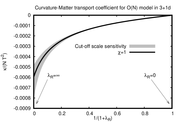
Figure 1: Transport coefficient $\kappa$ for the O(N) model in 3+1 dimensions in the large N limit as a function of coupling. Results are shown using a compactified interval $\frac{1}{1+\lambda_{R}}\in[0,1]$ in order to show all coupling values. Arrows indicate free theory and strong coupling limits, respectively. The band was generated by varying the scale through choosing $\chi\in[\frac{1}{2},2]$ in (16), in turn quantifying the sensitivity of $\kappa$ to the cut-off scale. See text for details.

Introducing an auxiliary field $\sigma=\frac{\vec{\phi}^{2}}{N}$ and Lagrange multiplier $\zeta$ and subsequently integrating out $\sigma$, the partition function $Z=\int{\cal D}\phi e^{-\int d^{4}x{\cal L}}$ can be rewritten as

$$Z=\int{\cal D}\phi{\cal D}\zeta e^{-\int d^{4}x\left[\frac{1}{2}\vec{\phi}\left(-\Box+i\zeta\right)\vec{\phi}+\frac{N\zeta^{2}}{16\lambda}\right]}\,.$$ (8)

In the large N limit, only the zero mode $\zeta_{0}$ contributes, and as a consequence the partition function can be calculated exactly from the location of the saddle at $i\zeta_{0}=z^{*}$,

$$Z = \sqrt{\frac{\beta VN}{16\lambda\pi}}\int d\zeta_{0}e^{-\beta VN\left[\frac{\zeta_{0}^{2}}{16\lambda}+J\left(\sqrt{i\zeta_{0}}\right)\right]}\,,$$ (9)

$$= e^{-\beta VN\left[J\left(\sqrt{z^{*}}\right)-\frac{z^{*2}}{16\lambda}\right]}\,,$$

where $V$ is the volume of ${\mathbb{R}}^{3}$, $J(m)\equiv T\sum_{\omega_{n}}\mu^{2\epsilon}\int\frac{d^{3-2\epsilon}}{(2\pi)^{3-2\epsilon}}\ln\left(\omega_{n}^{2}+m^{2}\right)$ in dimensional regularization Laine and Vuorinen (2016) and $\omega_{n}=2\pi nT$ are the bosonic Matsubara frequencies. (Note that this is completely analogous to the case of 2d and 3d discussed in Refs. Romatschke (2019a, b, c).) The two-point function thus becomes

$$\Delta(\omega_{n},{\bf k})=\frac{1}{\omega_{n}^{2}+{\bf k}^{2}+z^{*}}\,,$$ (10)

where the location of the saddle $z^{*}$ is given as the solution of the non-perturbative “gap-equation”

$$z^{*}=4\lambda I(\sqrt{z^{*}})\,.$$ (11)

Here $I(m)=2\frac{dJ(m)}{dm^{2}}=\,\hbox{$\sum$}\!\!\!\!\!\!\!\int\,_{k}[\omega_{n}^{2}+{\bf k}^{2}+m^{2}]^{-1}$ is a standard thermal integral found in textbooks such as Ref. Laine and Vuorinen (2016)

$$I(m)=-\frac{m^{2}}{16\pi^{2}\epsilon}-\frac{m^{2}}{16\pi^{2}}\ln\frac{\bar{\mu}^{2}e^{1}}{m^{2}}+\frac{mT}{2\pi^{2}}\sum_{n=1}^{\infty}\frac{K_{1}\left(\frac{nm}{T}\right)}{n}\,,$$ (12)

where $\bar{\mu}^{2}=4\pi\mu^{2}e^{-\gamma_{E}}$ is the renormalization scale parameter in the $\overline{\rm MS}$ scheme. Inspecting (11), one can non-perturbatively renormalize the theory by introducing a renormalized coupling constant $\lambda_{R}$ as

$$\frac{1}{\lambda_{R}}=\frac{1}{\lambda}+\frac{1}{4\pi^{2}\epsilon}\,.$$ (13)

This renormalization condition implies a positive $\beta$-function for all couplings. Integrating up the renormalization group equation gives

$$\frac{1}{\lambda_{R}(\bar{\mu})}=\frac{1}{4\pi^{2}}\ln\frac{\Lambda_{LP}^{2}}{\bar{\mu}^{2}}\,,$$ (14)

where $\Lambda_{LP}$ is the Landau pole of the theory (defined as the scale where $\lambda_{R}(\Lambda_{LP})=\infty$).

Expressing the thermal mass in (10) as $z^{*}=m_{B}^{2}T^{2}$, the dimensionless parameter $m_{B}$ is determined from (11) as

$$m_{B}=\frac{8\sum_{n}\frac{K_{1}\left(nm_{B}\right)}{n}}{\ln\frac{\Lambda_{LP}^{2}e^{1}}{m_{B}^{2}T^{2}}}=\frac{8\sum_{n}\frac{K_{1}\left(nm_{B}\right)}{n}}{\frac{4\pi^{2}}{\lambda_{R}}+\ln\frac{\bar{\mu}^{2}e^{1}}{m_{B}^{2}T^{2}}}\,,$$ (15)

either in terms of the ratio $\Lambda_{LP}/T$ or in terms of the renormalized running coupling. (Note that $m_{B}$ is independent from the choice of the renormalization scale parameter $\bar{\mu}$ as it should be for a physical observable.)

Note that while the gap equation (15) formally is well-defined for all temperature scales $T\in[0,\frac{\Lambda_{LP}}{2}]$, close to the Landau pole there will be modifications arising from radiative corrections to the effective theory Lagrangian. (This may be verified explicitly by adding a term such as $\frac{\lambda_{2}}{\Lambda_{LP}^{2}}\left(\vec{\phi}^{2}\right)^{3}$ to the Lagrangian (4), which is allowed for an UV-incomplete theory.) It is possible to test for the sensitivity to the cut-off scale by e.g. choosing units as

$$2\pi T=\frac{\Lambda_{LP}e^{-\frac{2\pi^{2}}{\lambda_{R}}}}{\chi}\,,$$ (16)

with fixed $\lambda_{R}$ and varying $\chi\in[\frac{1}{2},2]$.

In practice, the renormalized gap equation (15) possesses two solutions for $m_{B}$. Only the smaller one of these corresponds to a local minimum of the exponent, thus the larger one will be discarded in the following. The solution $m_{B}$ then fixes the form of the two-point function (10) non-perturbatively, and in turn allows calculation of the transport coefficient $\kappa$ from (5). Specifically, performing the angular averages in (6) leads to

$$\frac{\kappa}{2N}\equiv\frac{2}{105}\,\hbox{$\sum$}\!\!\!\!\!\!\!\int_{K}\left(4k^{6}\Delta^{4}(\omega_{n},k)-7k^{4}\Delta^{3}(\omega_{n},k)\right)+\frac{\xi}{2}I(m_{B}T)\,.$$ (17)

Inspecting this equation, one notices that the last term is divergent for $\epsilon\rightarrow 0$, cf. (12). Therefore, unless this divergence is exactly canceled by the other contributions, the result for $\kappa$ is meaningless. Using $\frac{\partial}{\partial m^{2}}\Delta=-\Delta^{2}$ repeatedly and performing a standard thermal sum, one finds

$$A=\,\hbox{$\sum$}\!\!\!\!\!\!\!\int_{K}k^{6}\Delta^{4}(\omega_{n},k) = -\frac{\partial^{3}}{(\partial z^{*})^{3}}\int_{k}\frac{k^{6}}{12E_{k}}\left(1+2n_{B}(E_{k})\right)\,,$$

$$B=\,\hbox{$\sum$}\!\!\!\!\!\!\!\int_{K}k^{4}\Delta^{3}(\omega_{n},k) = \frac{\partial^{2}}{(\partial z^{*})^{2}}\int_{k}\frac{k^{4}}{4E_{k}}\left(1+2n_{B}(E_{k})\right),\,\,\,$$ (18)

where $E_{k}=\sqrt{k^{2}+z^{*}}$ and $n_{B}(x)=\frac{1}{e^{x/T}-1}$. Expanding $n_{B}(x)=\sum_{n=1}^{\infty}e^{-n\beta x}$ both of the above integrals can be evaluated analytically, finding

$$4A = -\frac{35z^{*}}{64\pi^{2}}\left(\frac{1}{\epsilon}+\frac{37}{105}+\ln\frac{z^{*}}{\bar{\mu}^{2}}-8\sum_{n=1}^{\infty}\frac{K_{1}(n\beta\sqrt{z^{*}})}{n\beta}\right)\,,$$

$$7B = -\frac{105z^{*}}{128\pi^{2}}\left(\frac{1}{\epsilon}+\frac{1}{15}+\ln\frac{z^{*}}{\bar{\mu}^{2}}-8\sum_{n=1}^{\infty}\frac{K_{1}(n\beta\sqrt{z^{*}})}{n\beta}\right)\,.$$

Inserting these results into (17), I find that the $\epsilon\rightarrow 0$ divergence as well as the sums over Bessel functions both cancel for $\xi=\frac{1}{6}$, giving rise to the finite and simple result

$$\kappa=-\frac{13NT^{2}m_{B}^{2}}{2520\pi^{2}}\,,$$ (19)

with $m_{B}$ given by the solution of (15). This is the main result of this work. A quick cross-check reveals that in the free theory limit $\lambda_{R}\rightarrow 0$ Eq. (15) gives $m_{B}\rightarrow 0$, so that $\lim_{\lambda_{R}\rightarrow 0}\kappa=0$ (matching the result found in Ref. Kovtun and Shukla (2018) for a conformally coupled scalar).

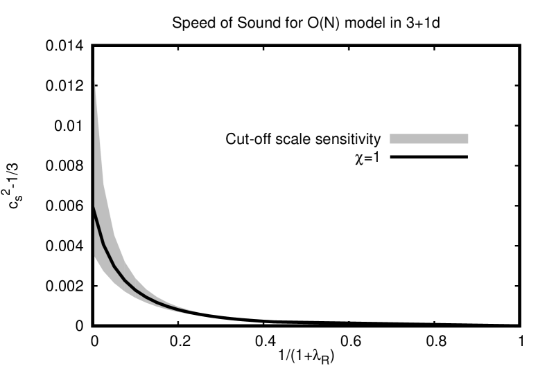
Figure 2: Speed of sound squared for the O(N) model in 3+1 dimensions in the large N limit as a function of coupling. Results are shown using a compactified interval $\frac{1}{1+\lambda_{R}}\in[0,1]$ in order to show all coupling values. The band was generated by varying the scale through choosing $\chi\in[\frac{1}{2},2]$ in (16), in turn quantifying the sensitivity of $c_{s}^{2}$ to the cut-off scale.

Of course, also thermodynamic properties of the O(N) model in 3+1 dimensions may be evaluated non-perturbatively along the same lines. For instance, the pressure (minus the free energy) is found from (9) as $P=\frac{\ln Z}{\beta V}$. It is worth pointing out that – using the explicit result Laine and Vuorinen (2016) for $J(m)=-\frac{m^{4}}{64\pi^{2}}\left[\frac{1}{\epsilon}+\ln\frac{\bar{\mu}^{2}e^{3/2}}{m^{2}}\right]-\frac{m^{2}T^{2}}{2\pi^{2}}\sum_{n}\frac{K_{2}\left(n\beta m\right)}{n^{2}}$ – the non-perturbative coupling renormalization (13) is sufficient to remove all divergences in the pressure (cf. Ref. Blaizot et al. (2001)), so that no counterterm for the cosmological constant is required. This leads to

$$P=\frac{NT^{4}}{64\pi^{2}}\left[m_{B}^{4}\ln\frac{\Lambda_{LP}^{2}e^{3/2}}{m_{B}^{2}T^{2}}+32m_{B}^{2}\sum_{n=1}^{\infty}\frac{K_{2}(nm_{B})}{n^{2}}\right]\,.$$ (20)

The entropy density $s\equiv\frac{\partial P}{\partial T}$ may be obtained most easily from (9) and (11), so that contributions proportional to $\frac{\partial z^{*}}{\partial T}$ cancel, leading to the result

$$s=\frac{NT^{3}m_{B}^{3}}{2\pi^{2}}\sum_{n=1}^{\infty}\frac{K_{3}(nm_{B})}{n}\,.$$ (21)

For weak coupling where $m_{B}\rightarrow 0$, $s\rightarrow s_{\rm free}=\frac{4NT^{3}\pi^{2}}{90}$, the well-known Stefan-Boltzmann result for a free theory.

From the thermodynamic relation $\epsilon+P=sT$ and this result, the trace anomaly can be evaluated to be

$$\epsilon-3P=-\frac{NT^{4}m_{B}^{4}}{32\pi^{2}}\,.$$ (22)

Note that the result is negative and that most contributions have canceled because of the gap equation (15). Finally, the speed of sound squared can be calculated as $c_{s}^{2}=\frac{s/T}{\frac{\partial s}{\partial T}}$, and evaluated numerically, see Fig. 2. Note that the speed of sound is very close to (and above) the conformal result $c_{s}^{2}=\frac{1}{3}$, which indicates that the O(N) model, though not a conformal theory (CFT), is numerically very close to a CFT for most coupling values. Indeed, it has not escaped my attention that the ratio $s/s_{\rm free}$ calculated from (21) seems to go to a constant value of approximately 85 percent for $\lambda_{R}\rightarrow\infty$ and $\chi=1$, very much in line with the universal strong-weak thermodynamic behavior found in 2+1d CFTs Romatschke (2019c); DeWolfe and Romatschke (2019).

One referee of this work remarked that for the O(N) model, $c_{s}^{2}\geq\frac{1}{3}$ while the authors of Ref. Hohler and Stephanov (2009) found that $c_{s}^{2}\leq\frac{1}{3}$ for a class of holographic theories. The apparent discrepancy can be understood to originate from the different sign of the $\beta$-function in scalar field theories (such as the O(N) model) and non-abelian gauge theories such as those considered in Ref. Hohler and Stephanov (2009). To take a simple example, let us consider the relation between the pressure and energy density in weakly coupled single-component $\phi^{4}$ theory, which can be obtained by combining results found in Ref. Laine and Vuorinen (2016) to give

$$P=\frac{\epsilon}{3}+\frac{T^{4}}{576}\frac{\partial\lambda}{\partial\ln T}+\ldots\,,$$ (23)

where $\frac{\partial\lambda}{\partial\ln T}$ is the $\beta$ function of $\phi^{4}$ theory. Since in scalar field theories, $\frac{\partial\lambda}{\partial\ln T}>0$, Eq. (23) implies $c_{s}^{2}\equiv\frac{dP}{d\epsilon}\geq\frac{1}{3}$, while for asymptotically free theories with negative $\beta$ function $c_{s}^{2}\leq\frac{1}{3}$.

III Discussion and Conclusions

The transport coefficient $\kappa$ given in (19) may be evaluated for any value of the renormalized coupling $\lambda_{R}$ by solving (15) numerically. The sensitivity to cut-off scale effects may be tested by the choice (16) through varying $\chi$. Results for $\kappa$ for all couplings are shown in Fig. 1. From this figure, it can be seen that cut-off scale sensitivity is minor (smaller than 10 percent) for $\lambda_{R}\lesssim 2.45$ and less than a factor of two even for $\lambda_{R}\rightarrow\infty$. This compares favorably with the situation found for the QCD shear viscosity calculated to NLO in perturbation theory Ghiglieri et al. (2018). The weak sensitivity to cut-off scale effects suggests that the result (19) constitutes an example of a transport coefficient that is known non-perturbatively for a large range of coupling values. As such, this example may be useful for instance for testing approximation techniques (either at weak or at strong coupling), or conceivably in early-time cosmology where curvature matter couplings will play an important role in the dynamics.

The results found in this work are exact only in the strict large N limit. However, based on the non-perturbative results for scalar theory in 1+1d in Ref. Romatschke (2019b), I conjecture that the large N results in this work constitute quantitatively good approximations for finite N at arbitrary coupling, including N=1 scalar $\phi^{4}$ theory.

Is it possible to non-perturbatively evaluate other transport coefficients in a similar manner? The answer to this question likely is affirmative since other channels of the energy-momentum tensor two-point function couple to transport coefficients such as $\kappa^{*},\xi_{5},\xi_{6}$ in a similar manner, cf. Refs. Romatschke and Romatschke (2019); Moore and Sohrabi (2012); Kovtun and Shukla (2018) for details.

It would also be interesting to extend this work on the O(N) model and study non-perturbative relations between $\kappa,\kappa^{*}$ and the shear viscosity coefficient discussed in Ref. Kleinert and Probst (2016), or the Haack-Yarom relation Haack and Yarom (2009), which has been investigated extensively in holographic theories Grozdanov and Starinets (2015).

It is my hope that this work could instill interest and further progress in the field of non-perturbative transport calculations.

IV Acknowledgments

This work was supported by the Department of Energy, DOE award No DE-SC0017905. I would like to thank S.P. de Alwis, T. DeGrand, S. Grozdanov, P. Kovtun and G. Moore for helpful discussions.

References

- Bhattacharyya et al. (2008) Sayantani Bhattacharyya, Veronika E Hubeny, Shiraz Minwalla, and Mukund Rangamani, “Nonlinear Fluid Dynamics from Gravity,” JHEP 02, 045 (2008), arXiv:0712.2456 [hep-th] .
- Baier et al. (2008) Rudolf Baier, Paul Romatschke, Dam Thanh Son, Andrei O. Starinets, and Mikhail A. Stephanov, “Relativistic viscous hydrodynamics, conformal invariance, and holography,” JHEP 04, 100 (2008), arXiv:0712.2451 [hep-th] .
- Romatschke and Romatschke (2019) Paul Romatschke and Ulrike Romatschke, Relativistic Fluid Dynamics In and Out of Equilibrium, Cambridge Monographs on Mathematical Physics (Cambridge University Press, 2019) arXiv:1712.05815 [nucl-th] .
- Romatschke and Son (2009) Paul Romatschke and Dam Thanh Son, “Spectral sum rules for the quark-gluon plasma,” Phys. Rev. D80, 065021 (2009), arXiv:0903.3946 [hep-ph] .
- Moore and Sohrabi (2012) Guy D. Moore and Kiyoumars A. Sohrabi, “Thermodynamical second-order hydrodynamic coefficients,” JHEP 11, 148 (2012), arXiv:1210.3340 [hep-ph] .
- Finazzo et al. (2015) Stefano I. Finazzo, Romulo Rougemont, Hugo Marrochio, and Jorge Noronha, “Hydrodynamic transport coefficients for the non-conformal quark-gluon plasma from holography,” JHEP 02, 051 (2015), arXiv:1412.2968 [hep-ph] .
- Grozdanov and Starinets (2017) Sašo Grozdanov and Andrei O. Starinets, “Second-order transport, quasinormal modes and zero-viscosity limit in the Gauss-Bonnet holographic fluid,” JHEP 03, 166 (2017), arXiv:1611.07053 [hep-th] .
- Philipsen and Schäfer (2014) Owe Philipsen and Christian Schäfer, “The second order hydrodynamic transport coefficient for the gluon plasma from the lattice,” JHEP 02, 003 (2014), arXiv:1311.6618 [hep-lat] .
- Jeon (1995) Sangyong Jeon, “Hydrodynamic transport coefficients in relativistic scalar field theory,” Phys. Rev. D52, 3591–3642 (1995), arXiv:hep-ph/9409250 [hep-ph] .
- Arnold et al. (2003) Peter Brockway Arnold, Guy D Moore, and Laurence G. Yaffe, “Transport coefficients in high temperature gauge theories. 2. Beyond leading log,” JHEP 05, 051 (2003), arXiv:hep-ph/0302165 [hep-ph] .
- Moore (2007) Guy D. Moore, “Next-to-Leading Order Shear Viscosity in lambda phi**4 Theory,” Phys. Rev. D76, 107702 (2007), arXiv:0706.3692 [hep-ph] .
- Ghiglieri et al. (2018) Jacopo Ghiglieri, Guy D. Moore, and Derek Teaney, “QCD Shear Viscosity at (almost) NLO,” JHEP 03, 179 (2018), arXiv:1802.09535 [hep-ph] .
- Policastro et al. (2001) G. Policastro, Dan T. Son, and Andrei O. Starinets, “The Shear viscosity of strongly coupled N=4 supersymmetric Yang-Mills plasma,” Phys. Rev. Lett. 87, 081601 (2001), arXiv:hep-th/0104066 [hep-th] .
- Kats and Petrov (2009) Yevgeny Kats and Pavel Petrov, “Effect of curvature squared corrections in AdS on the viscosity of the dual gauge theory,” JHEP 01, 044 (2009), arXiv:0712.0743 [hep-th] .
- Buchel (2008) Alex Buchel, “Resolving disagreement for eta/s in a CFT plasma at finite coupling,” Nucl. Phys. B803, 166–170 (2008), arXiv:0805.2683 [hep-th] .
- Moore (2001) Guy D. Moore, “Transport coefficients in large N(f) gauge theory: Testing hard thermal loops,” JHEP 05, 039 (2001), arXiv:hep-ph/0104121 [hep-ph] .
- Aarts and Martinez Resco (2005) Gert Aarts and Jose M. Martinez Resco, “Transport coefficients in large N(f) gauge theories with massive fermions,” JHEP 03, 074 (2005), arXiv:hep-ph/0503161 [hep-ph] .
- Meyer (2007) Harvey B. Meyer, “A Calculation of the shear viscosity in SU(3) gluodynamics,” Phys. Rev. D76, 101701 (2007), arXiv:0704.1801 [hep-lat] .
- Borsányi et al. (2018) Sz. Borsányi, Zoltan Fodor, Matteo Giordano, Sandor D. Katz, Attila Pasztor, Claudia Ratti, Andreas Schäfer, Kalman K. Szabo, and Balint C. Toth, “High statistics lattice study of stress tensor correlators in pure gauge theory,” Phys. Rev. D98, 014512 (2018), arXiv:1802.07718 [hep-lat] .
- Kovtun and Shukla (2018) Pavel Kovtun and Ashish Shukla, “Kubo formulas for thermodynamic transport coefficients,” JHEP 10, 007 (2018), arXiv:1806.05774 [hep-th] .
- Parker and Toms (2009) Leonard E. Parker and D. Toms, Quantum Field Theory in Curved Spacetime, Cambridge Monographs on Mathematical Physics (Cambridge University Press, 2009).
- Laine and Vuorinen (2016) Mikko Laine and Aleksi Vuorinen, “Basics of Thermal Field Theory,” Lect. Notes Phys. 925, pp.1–281 (2016), arXiv:1701.01554 .
- Romatschke (2019a) Paul Romatschke, “Simple non-perturbative resummation schemes beyond mean-field: case study for scalar theory in 1+1 dimensions,” JHEP 03, 149 (2019a), arXiv:1901.05483 [hep-th] .
- Romatschke (2019b) Paul Romatschke, “Simple non-perturbative resummation schemes beyond mean-field II: thermodynamics of scalar theory in 1+1 dimensions at arbitrary coupling,” (2019b), arXiv:1903.09661 [hep-th] .
- Romatschke (2019c) Paul Romatschke, “Finite-Temperature Conformal Field Theory Results for All Couplings: O(N) Model in 2+1 Dimensions,” Phys. Rev. Lett. 122, 231603 (2019c), arXiv:1904.09995 [hep-th] .
- Blaizot et al. (2001) J. P. Blaizot, Edmond Iancu, and A. Rebhan, “Approximately selfconsistent resummations for the thermodynamics of the quark gluon plasma. 1. Entropy and density,” Phys. Rev. D63, 065003 (2001), arXiv:hep-ph/0005003 [hep-ph] .
- DeWolfe and Romatschke (2019) Oliver DeWolfe and Paul Romatschke, “Strong Coupling Universality at Large N for Pure CFT Thermodynamics in 2+1 dimensions,” (2019), arXiv:1905.06355 [hep-th] .
- Hohler and Stephanov (2009) Paul M. Hohler and Mikhail A. Stephanov, “Holography and the speed of sound at high temperatures,” Phys. Rev. D80, 066002 (2009), arXiv:0905.0900 [hep-th] .
- Kleinert and Probst (2016) Philipp Kleinert and Jonas Probst, “Second-Order Hydrodynamics and Universality in Non-Conformal Holographic Fluids,” JHEP 12, 091 (2016), arXiv:1610.01081 [hep-th] .
- Haack and Yarom (2009) Michael Haack and Amos Yarom, “Universality of second order transport coefficients from the gauge-string duality,” Nucl. Phys. B813, 140–155 (2009), arXiv:0811.1794 [hep-th] .
- Grozdanov and Starinets (2015) Sašo Grozdanov and Andrei O. Starinets, “On the universal identity in second order hydrodynamics,” JHEP 03, 007 (2015), arXiv:1412.5685 [hep-th] .