Dynamic mode decomposition for analytic maps

Abstract

Extended dynamic mode decomposition (EDMD) provides a class of algorithms to identify patterns and effective degrees of freedom in complex dynamical systems. We show that the modes identified by EDMD correspond to those of compact Perron-Frobenius and Koopman operators defined on suitable Hardy-Hilbert spaces when the method is applied to classes of analytic maps. Our findings elucidate the interpretation of the spectra obtained by EDMD for complex dynamical systems. We illustrate our results by numerical simulations for analytic maps.

1 Introduction

The quest to identify effective degrees of freedom in a complex dynamical system is a fundamental topic in almost all branches of science. The archetype and historical origin of this endeavour can be seen in the derivation of thermodynamics from microscopic equations of motion within a hydrodynamic description. Here, the relevant macroscopic densities are determined by the classical conservation laws of physics. In a mathematical setting the problem of identifying effective degrees of freedom and reducing the dynamical description to a lower dimensional set of equations can be cast in terms of centre manifold reductions [14] or adiabatic elimination procedures [15]. In these classical situations the reduction of the description to effective degrees of freedom has resulted in the derivation of transport equations for systems far from equilibrium using projection operator techniques [23, 32], an understanding of how dissipation emerges in many particle Hamiltonian systems [24], or the Bandtlow-Coveney equation for transport properties in discrete-time dynamical systems [2], to name but a few. With the advent of the study of complex and chaotic dynamical behaviour the focus has shifted and broadened. Nowadays the problem of identifying relevant degrees of freedom occupies a diverse range of scientific fields ranging from physics and the life sciences, to computational studies of pattern recognition or data processing. Many of the current algorithmic approaches have been inspired by the classical ideas mentioned above. In a nutshell, these methods are based on identifying an optimal mode decomposition which can be used to effectively describe the system of interest.

A recent instalment of these ideas has become known as Dynamic Mode Decomposition, introduced in [27] and extended in [31]; see also [18] for an illustration of this concept in the context of nonlinear stochastic systems. At their core, these methods condense the dynamical observations into a suitably chosen effective linear evolution matrix. The eigenvalues and eigenvectors of this matrix then provide information concerning the relevance and structure of the effective degrees of freedom of the system, and can sometimes be related to spectral data of global evolution operators, known as Perron-Frobenius operators, or their formal adjoints, known as Koopman operators. Data-driven methods to approximate Perron-Frobenius and Koopman operators have become prominent with the work of Dellnitz and Junge [9] and have since been extended in many ways [8, 11, 22, 13, 17], to mention but a few. For an overview of existing algorithms, see the review articles [19, 7, 13] and references therein, in particular [19] for comparison of various data-driven algorithms, [7] for an overview of applications in areas of engineering, and the introductory section of [13] for a historical overview.

Empirically, these algorithms perform extremely well and are essentially fully understood for finite-dimensional linear dynamical systems. However, open questions remain in more complex dynamical setups, regarding, for example, under which conditions the algorithms converge and whether the limiting quantities are signatures of the underlying dynamical system in the sense that they approximate the spectral data of the relevant evolution operator. In this note our aim is to contribute to this issue, by proving that a certain version of dynamic mode decomposition, known as Extended Dynamic Mode Decompostion (EDMD), identifies the correct effective degrees of freedom in an analytic setup when certain classes of deterministic chaotic dynamical systems are studied.

In order to keep our presentation self-contained we start with a brief sketch of EDMD in Section 2. In Section 3 we introduce a class of analytic circle maps, for which rigorous statements about EDMD can be made. For this class of systems we show that EDMD singles out eigenmodes of the Perron-Frobenius operator on a suitably defined space of analytic functions. In this sense EDMD effectively performs a coarse graining or smoothing of the dynamics. We shall also explain that, in an appropriate setting, these results translate into strong spectral convergence results for the corresponding Koopman operator. In Section 4 we illustrate our findings through various numerical examples based on exactly solvable models. Finally, in Section 5, we put our results in a more general context, including a discussion of higher dimensional dynamical systems or the relevance of our rigorous approach for general dynamic mode decompositions where no proofs can be provided.

2 Extended Dynamic Mode Decomposition

In the following, we shall provide a brief, informal account of Extended Dynamic Mode Decomposition (EDMD). Consider a discrete dynamical system

$$z_{n+1}=\tau(z_{n})\,$$ (1)

given by map a $\tau\colon\mathcal{X}\to\mathcal{X}$ on some phase space $\mathcal{X}$. Assume that the dynamics is observed through a collection of $N$ scalar functions defined on the phase space given by $\psi(z)=(\psi_{1}(z),\ldots,\psi_{N}(z))^{T}$. We record the dynamics at a sequence of $M$ phase space points $z^{(1)},\ldots,z^{(M)}$. These points can be obtained from a time series if the approach is used as a data analysis tool, or as a sample from a suitable distribution of points in phase space if the goal is to investigate the underlying equations of motion (1). Glossing over details of the underlying theory (see for example, [31, 18, 17, 20] and references therein), the fundamental quantity of EDMD is an $N\times N$ matrix

$$A=GH^{-1},$$ (2)

which is constructed from the observations as follows

$$G_{kl}= \frac{1}{M}\sum_{m=1}^{M}\psi_{k}(\tau(z^{(m)}))\psi_{l}(z^{(m)})\,, (k,l=1,\ldots,N)\,,$$ (3)

$$H_{kl}= \frac{1}{M}\sum_{m=1}^{M}\psi_{k}(z^{(m)})\psi_{l}(z^{(m)})\,, (k,l=1,\ldots,N)\,.$$ (4)

Given the observations, the matrix $A$ is an optimal representation of the dynamics in terms of a finite dimensional linear equation of motion in the following sense: it is a least squares solution to $AX=Y$ where $X=[\psi(z^{(1)}),\dots,\psi(z^{(M)})]$ and $Y=[\psi(\tau(z^{(1)})),\dots,\psi(\tau(z^{(M)}))]$. For sufficiently large values of $M$ and $N$ the eigenvalues and eigenvectors of $A$ determine the effective modes of the system. Eigenmodes with eigenvalues on or close to the complex unit circle are the slow modes which are relevant for macroscopic behaviour and the long term dynamics.

The matrix $A$ can be linked to the linear operator governing the underlying dynamics (1), the Perron-Frobenius operator, or its formal adjoint, the Koopman operator. Previous investigations [20] have shown that in the limit of large $N$ and $M$ the matrix $A$ is, in a certain sense, a suitable matrix representation, provided strong technical conditions are met. These conditions, however, may be difficult to verify in concrete applications.

Numerical results show that EDMD can often be applied successfully as a practical algorithm and indicate that output data (for example, eigenvalues of $A$) exhibit nice convergence properties. We will prove that this is indeed the case for a suitable class of dynamical systems, which will be introduced in the next section.

3 EDMD for analytic maps

Let us consider a full branch analytic expanding map on an interval, say $[0,2\pi]$. Using the canonical mapping $\varphi\mapsto z=\exp(i\varphi)$ this map can be viewed as a map $\tau$ in the complex plane leaving the unit circle $\mathbb{T}=\{z\in\mathbb{C}:|z|=1\}$ invariant. The map $\tau$ will be analytic on $\mathbb{T}$, provided that the branches of the original map on $[0,2\pi]$ satisfy matching conditions at the endpoints, and will thus have an analytic extension to an open annulus $\mathbb{A}$ containing $\mathbb{T}$. This means that such a map admits a Laurent series on $\mathbb{A}$ which, on the unit circle, coincides with the Fourier series expansion of the original interval map. Moreover, the Fourier coefficients will decay exponentially. This last property is one of the crucial ingredients that will allow us to define the evolution operators on sufficiently nice function spaces, as discussed below. The second crucial ingredient is the expansivity of the map, by which we mean that $|\tau^{\prime}(z)|>1$ for all $z\in\mathbb{T}$.

The fine statistical properties of the map $\tau$ are captured by the Perron-Frobenius operator (or transfer operator), which describes the forward evolution of densities under the action of the system. For analytic expanding (orientation-preserving) circle maps, it takes the form

$$(\mathcal{L}f)(z)=\sum_{j}\phi_{j}^{\prime}(z)f(\phi_{j}(z)),$$ (5)

where $\phi_{j}$ denotes the $j$-th inverse branch of the analytic map $\tau$. For instance, for the simple Bernoulli shift map $\varphi\mapsto 2\varphi\mbox{ mod }2\pi$, the corresponding circle map reads $\tau(z)=z^{2}$ with the two inverse branches given by $\phi_{1}(z)=\sqrt{z}$ and $\phi_{2}(z)=-\sqrt{z}$.

The operator in (5) is naturally defined on $L^{1}(\mathbb{T})$, the positive elements of which are interpretable as probability densities, but for convenience it is often considered as an operator restricted to $L^{2}(\mathbb{T})$ so that Hilbert space methods can be used. Its adjoint is known as the Koopman operator, which turns out to be the operator of composition with the map $\tau$. However, the Hilbert space $L^{2}(\mathbb{T})$ is “fairly large” so that the spectrum of the bounded operator $\mathcal{L}$ is the entire closed complex unit disk, with each point in the open unit disk being an eigenvalue of infinite multiplicity (see, for example, [16, Remark 4.4]). Intuitively, the function space $L^{2}(\mathbb{T})$ simply contains too many “non-physical” observables.

In order to capture the behaviour observed in a time series one often restricts the set of observables, that is, one takes a suitable subspace of $L^{2}(\mathbb{T})$, so that decay rates show up as isolated spectral points of the Perron-Frobenius operator. In a sense such a restriction corresponds to the coarse graining used in statistical mechanics when moving from a conservative microscopic to a dissipative hydrodynamic description [24]. An elementary illustration of this aspect can be found for instance in [26].

Spectral convergence. In order to obtain strong spectral results for our setup of analytic circle maps, a suitable class of observables is a space of analytic functions. Following the approach in [5] we restrict observables to be analytic functions on an open annulus $\mathbb{A}$ containing the complex unit circle with an $L^{2}$-extension to the boundary of $\mathbb{A}$, the so-called Hardy-Hilbert space $H^{2}(\mathbb{A})$. As shown in [5], the Perron-Frobenius operator given by (5) considered on $H^{2}(\mathbb{A})$ is well-defined and compact, which implies that it has a discrete spectrum of eigenvalues which govern the correlation decay and the relaxation of analytic observables.

In addition, the Perron-Frobenius operator can be effectively approximated by a sequence of finite rank operators. For this consider an orthogonal basis of the underlying Hardy-Hilbert space, for instance, the canonical (non-normalised) orthogonal basis $\psi_{m}(z)=z^{m}$ with $m\in\mathbb{Z}$. The corresponding matrix elements of the operator in (5) are then given by

$$L_{kl}=\frac{1}{2\pi}\int_{0}^{2\pi}\psi_{k}(\tau(\exp(i\varphi)))\psi_{l}(\exp(i\varphi))\,d\varphi\,.$$ (6)

The matrix elements with $k,l=-\bar{N},\ldots,\bar{N}$ yield an $N\times N$ matrix representation of a finite rank approximation of the Perron-Frobenius operator, with $N=2\bar{N}+1$. It has been shown in [5] that these approximations converge to the Perron-Frobenius operator exponentially fast in operator norm. Hence, the eigenvalues of the matrices of size $N\times N$ approximate the spectrum of the infinite-dimensional compact operator ${\mathcal{L}}$ as $N$ tends to infinity. Moreover, convergence of the eigenvalues occurs at an exponential rate and explicit error bounds can be derived from the general theory. In summary, a finite dimensional matrix approximation using (6) provides the spectrum of the compact Perron-Frobenius operator and that of its adjoint.

More formally, the results can be stated as follows

.

Let $\tau$ be an analytic expanding circe map, and $\mathcal{L}$ the corresponding Perron- Frobenius operator, given by (5). Denote by $\{\psi_{m}\}_{m\in\mathbb{Z}}$ with $\psi_{m}(z)=z^{m}$ the canonical orthogonal basis in $H^{2}(\mathbb{A})$and let $P_{N}$ be the orthogonal projection operator onto the subspace spanned by $\psi_{-\bar{N}},\ldots,\psi_{\bar{N}}$, where $N=2\bar{N}+1$.

1. (Compactness of $\mathcal{L}$)
   The operator $\mathcal{L}$ is a well-defined, compact operator from $H^{2}(\mathbb{A})$  to itself.

2. (Matrix representation)
   A matrix representation of the finite rank operator $P_{N}\mathcal{L}P_{N}$ is given by $(M_{kl})_{k,l}$ with $k,l=-\bar{N},\ldots,\bar{N}$ and $M_{kl}=L_{-k,l}$ as in (6).

3. (Convergence in operator norm)
   $||\mathcal{L}-P_{N}\mathcal{L}P_{N}||_{H^{2}(\mathbb{A})\to H^{2}(\mathbb{A})}=O(\exp(-aN))$ for some $a>0$.

4. (Eigenvalue convergence)
   The spectrum $\sigma(\mathcal{L})$ of $\mathcal{L}$ consists of at most countably many non-zero eigenvalues $\lambda_{n}$ of finite multiplicity, with $0$ the only possible accumulation point.

   1. If $(\lambda^{(N)})_{N\in\mathbb{N}}$ with $\lambda^{(N)}\in\sigma(P_{N}\mathcal{L}P_{N})$ is a convergent sequence, that is, $\lambda^{(N)}\to\lambda$, then $\lambda\in\sigma(\mathcal{L})$.

   2. For every $\lambda\in\sigma(\mathcal{L})$ there exists a sequence $(\lambda^{(N)})_{N\in\mathbb{N}}$ with $\lambda^{(N)}\in\sigma(P_{N}\mathcal{L}P_{N})$, such that $\lambda^{(N)}\to\lambda$.

   More precisely, for suitable enumerations $\lambda_{n}$ with $n\in\mathbb{N}_{0}$ of the respective non-zero eigenvalues (taking algebraic multiplicities into account) of $P_{N}\mathcal{L}P_{N}$ and $\mathcal{L}$, we have: for every $n$

   $$|\lambda_{n}(P_{N}\mathcal{L}P_{N})-\lambda_{n}(\mathcal{L})|=O(\exp(-aN))\quad\text{as $N\to\infty$}$$ (7)

   for some $a>0$.

In practical applications, a-priori error bounds for (7) can be computed explicitly using [3].

For the proof of the above, observe that (a) follows from [5, Proposition 3.4] and (c) is implied by the proof of [5, Lemma 3.3]. Item (b) follows from a calculation using duality (see, for example, [28, Lemma 2.3]) and the inner product of $H^{2}(\mathbb{A})$  from [5]. Items (i) and (ii) of (d) are known as Properties U and L in [1], and follow from Corollaries 2.7 and 2.13 therein, respectively. Finally, the exponential convergence of eigenvalues in (7) is an immediate consequence of [1, Theorem 2.18] and the ensuing remarks, combined with (c).

The relation between Perron-Frobenius and Koopman operators. We have chosen to present our results formulated for the Perron-Frobenius operator. A large part of the literature on data-driven methods such as EDMD is based on the study of the Koopman operator, given by $f\mapsto f\circ\tau$, which is the adjoint of the Perron-Frobenius operator when viewed on $L^{2}(\mathbb{T})$. In order to obtain the strong spectral convergence results described above, it was necessary to restrict the domain of the Perron-Frobenius operator to the “smaller space” $H^{2}(\mathbb{A})$. This space is densely and continuously embedded in $L^{2}(\mathbb{T})$, and thus an example of a test function space (see, for example, [30]), so that we have

$$H^{2}(\mathbb{A})\subset L^{2}(\mathbb{T})\simeq L^{2}(\mathbb{T})^{\prime}\subset{H^{2}(\mathbb{A})^{\prime}},$$ (8)

where $H^{2}(\mathbb{A})^{\prime}$ is the topological dual of $H^{2}(\mathbb{A})$. The structure (8) is known as a rigged Hilbert space or Gelfand triple (see, for example, [12] or [6]), which has been used in the context of dynamical systems to study spectral decompositions for certain chaotic maps (see, for example, [4] and references therein). The (Banach space) adjoint of the Perron-Frobenius operator $\mathcal{L}$ restricted to a “small space” $H^{2}(\mathbb{A})$  can be identified with a Koopman operator extended to a “large space” $H^{2}(\mathbb{A})^{\prime}$, on which it is compact.

Moreover, it turns out that in our setting of analytic expanding circle maps, it is even possible to identify this extended operator on $H^{2}(\mathbb{A})^{\prime}$ with certain Koopman operators acting on spaces of analytic functions. As was shown in [5], the space $H^{2}(\mathbb{A})^{\prime}$ can be identified with the space of functions holomorphic on two disks comprising the complement of the annulus $\mathbb{A}$, denoted $H^{2}(\mathbb{D}_{in})\oplus H_{0}^{2}(\mathbb{D}_{out})$. Consequently, the expression (6) also yields the matrix representation of the Koopman operator on this space.

Spectral convergence for EDMD. The results above imply that for analytic circle maps, EDMD has strong convergence properties and captures the spectrum of the associated Perron-Frobenius and Koopman operators. For a suitable choice of sampling points $z^{(m)}$ the expression (3) estimates the matrix elements (6), as established in [31] (see also [18] or [20]). For instance, when choosing equidistant points on the unit circle, $z^{(m)}=\exp(2\pi im/M)$, the expression (3) converges exponentially in $M$ to the integral (6). The matrix $H$ in (4) takes account of the orthonormalisation of the observables which was used in writing down the matrix elements (6). Hence, EDMD with equidistant sample points applied to analytic circle maps with analytic observables gives precisely the spectrum of the corresponding compact Perron-Frobenius and Koopman operators. Thus, EDMD singles out the physically observable decay rates and the corresponding dissipative modes. We will illustrate this result in the next section by analytically solvable examples and extend some of the results for the use of actual time series analysis.

4 Exactly solvable models

In order to illustrate the convergence properties of EDMD, analytic maps with accessible point spectrum are needed. Although the Perron-Frobenius operator and its adjoint are compact on Hardy-Hilbert spaces, computing their eigenvalues remains a challenging task. The first nontrivial family of analytic maps with explicitly computable spectrum has been identified in [28]. The family comprises circle maps $\tau$ which analytically extend to a neighbourhood of the entire unit disk (not just an annulus), that is, maps arising from Blaschke products. For these maps, the entire spectrum of the Perron-Frobenius operator is determined by fixed point properties of $\tau$ inside the unit disk [5].

To be more explicit consider a Blaschke product of degree two, given by

$$\tau(z)=\frac{z-\mu}{1-\bar{\mu}z}\frac{z-\rho}{1-\bar{\rho}z},\quad|\mu|,|\rho|<1,$$ (9)

with two complex-valued parameters $\mu=|\mu|\exp(i\alpha)$ and $\rho=|\rho|\exp(i\beta)$, where $\bar{\mu}$ and $\bar{\rho}$ denote the complex conjugates of $\mu$ and $\rho$, respectively. This map preserves the unit circle, where (considered in angular coordinates) it induces a two-branch interval map

$$\varphi\mapsto 2\varphi +2\mbox{arctan}\left(\frac{|\mu|\sin(\varphi-\alpha)}{1-|\mu|\cos(\varphi-\alpha)}\right)$$

$$+2\mbox{arctan}\left(\frac{|\rho|\sin(\varphi-\beta)}{1-|\rho|\cos(\varphi-\beta)}\right)\quad(\mbox{mod }2\pi)\,.$$ (10)

The map (4) can be considered as an analytic deformation of the Bernoulli shift map which is obtained for the choice $\mu=\rho=0$. The map $\tau$ is eventually expanding on the unit circle if and only if [25, Propositions 2.1, 3.1] it has a unique (attracting) fixed point $z_{*}=\tau(z_{*})$ in the unit disk, that is, $|z_{*}|<1$. As shown in [5], the powers of the multiplier $\tau^{\prime}(z_{*})$ and their complex conjugates are precisely the eigenvalues $\lambda_{n}$ of the Perron-Frobenius operator

$$\lambda_{0}=1,\quad\lambda_{2n-1}=(\tau^{\prime}(z_{*}))^{n},\quad\lambda_{2n}=(\overline{\tau^{\prime}(z_{*})})^{n},\quad n\in\mathbb{N}\,.$$ (11)

We use the map (9) to illustrate EDMD with a set of analytic observables. An obvious choice is the set of the first $\bar{N}$ Fourier modes, that is, $\{\psi_{k}(z)=z^{k}:-\bar{N}\leq k\leq\bar{N}\}$ using complex notation $z=\exp(i\varphi)$. Furthermore, as mentioned in the previous section we evaluate (3) and (4) for equidistant nodes on the unit circle $z^{(m)}=\exp(2\pi im/M)$ with $m=0,\ldots,M-1$. It is straightforward to show that our observables are orthogonal in the sense that $H_{k\ell}=\delta_{k,-\ell}$ in (4), if the number of nodes exceeds the number of observables, $M\geq N=2\bar{N}+1$. It remains to evaluate (3), for which we will consider maps of the form (9).

Let us first comment on the trivial parameter choice $\mu=\rho=0$, that is, on the Bernoulli shift map. Clearly $\tau(z)=z^{2}$ has fixed point $z_{*}=0$ with multiplier $\tau^{\prime}(z_{*})=0$, so all eigenvalues of the Perron-Frobenius operator in (11) apart from $\lambda_{0}$ vanish. For the application of EDMD, equation (3) can be easily evaluated to yield $G_{k\ell}=\delta_{-2k,\ell}$, as long as the number of nodes is sufficiently large, that is, $M\geq 3N/2$. Then the matrix $A=GH^{-1}$ is given by $A_{k\ell}=\delta_{2k,\ell}$ and its eigenvalues in fact coincide with the leading part of the exact spectrum given by (11).

For any non-trivial Blaschke map, the sums in (3) and the related finite-dimensional eigenvalue problem need to be evaluated numerically. For that purpose we set $\mu=\rho=0.33\cdot\exp(i\pi/25)$ which results in a spectrum with a fairly rich structure, so it can serve as a test for the efficiency of EDMD. Figure 1 shows the eigenvalues of $A$ for $M=100$ equidistant nodes, $N=11$ and $N=21$ observables compared with the exact expression (11). A set of $N=11$ modes are just sufficient to approximate the subleading complex eigenvalue pair ($\lambda_{1}$ and $\lambda_{2}=\bar{\lambda}_{1}$) while all the other values are spurious results. For a higher number of modes, $N=21$, about a quarter of the eigenvalues of $A$ give reasonable estimates of the correct spectrum. In particular, EDMD reproduces the leading part of the spectrum of the compact Perron-Frobenius operator as asserted in Section 3.

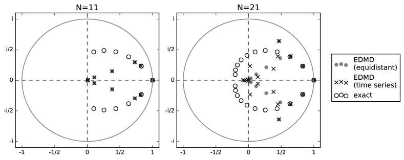
Figure 1: Complex plane with exact eigenvalues (open symbols) and approximation by EDMD with $M=100$ equidistant nodes (full symbols) or by EDMD applied to time series of length $M=5\cdot 10^{4}$ (crosses) for the Blaschke product in (9), with $\mu=\rho=0.33\cdot\exp(i\pi/25)$ for $N=11$ modes (left) or $N=21$ modes (right).

The dependence of the numerical error on the order $N$ of the eigenvalue approximation is shown in Figure 2. As we want to disentangle the effect of the two parameters, $M$ and $N$, we take $M$ large enough, $M=1000$, so that all matrix elements of the finite rank approximation $P_{N}\mathcal{L}P_{N}$ are estimated by the sums (3) sufficiently accurately. Hence any visible error is due to the finite mode approximation. An exponential decay (in $N$) of the eigenvalue approximation error is clearly observable.

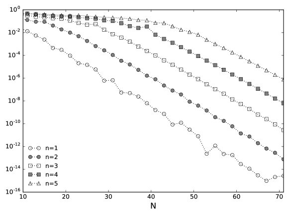
Figure 2: Absolute error of the first five subleading complex-conjugate eigenvalue pairs $(\lambda_{2n-1},\lambda_{2n})$ computed by EDMD (with $M=1000$ nodes) for a Blaschke product (9), with $\mu=\rho=0.33\cdot\exp(i\pi/25)$, as a function of the number of observables $N$.

5 Discussion

We have shown that EDMD singles out eigenvalues of compact Perron-Frobenius or Koopman operators arising in an analytic setting. Moreover, the algorithm converges at an exponential rate in the number of observables used.

EDMD as a data analysis tool. So far we have focussed on equidistant points in phase space to evaluate EDMD. In applications one normally resorts to an actual time series. If we reconsider the setup used for Figure 1 but now take nodes generated from a time series, that is, $z^{(m)}=z_{m}=\tau(z_{m-1})$, we still obtain an accurate approximation of the spectrum of the Perron-Frobenius operator (see crosses in Figure 1), as long as we minimise statistical fluctuations in the sums (3) and (4) by taking a time series of sufficient length. In fact, a slight modification of the arguments presented in Section 3 allows one to base the matrix elements (6) on integrals with respect to the analytic invariant density instead of the Lebesgue measure. Whereas the matrix entries in (6) change, the convergence results remain unaffected. In particular, EDMD exhibits the same convergence, when used as a time series analysis tool.

Convergence in $M$ and $N$. Our approach is based on finite rank operators represented by (6) converging in operator norm to a compact transfer operator. The nodes used in EDMD, in (3) and (4), can naturally be considered as a sampling of the corresponding integral. However, a rigorous estimate which involves both quantities, $M$ and $N$, appears to require taking the limit of large $M$ first. This may in fact not be necessary. While the approach so far was based on using orthogonal projectors, one can in fact directly link the matrix representation involving sums with a compact transfer operator by employing non-orthogonal projectors arising from collocation methods. It may thus be possible to show convergence for the case of $M$ and $N$ of the same order.

Higher dimensional extensions and multifractal properties. So far one may object that we have enforced an analytic setting and that the results are not really surprising as the maps do not allow for any complex multifractal behaviour. This is in fact not correct as analyticity is only required for the actual equation of motion, whereas the relevant invariant measure itself could be singular with respect to the phase space volume. In order to demonstrate this phenomenon, we resort to analytical solutions of two-dimensional hyperbolic diffeomorphisms which allow for fractal invariant measures if the Jacobian is not constant. The presence of contracting and expanding directions requires using more involved function spaces, that is, a particular class of anisotropic Hilbert spaces, for which rigorous statements on spectral data of evolution operators are possible (see, for example, [29] for technical details). We illustrate our point by considering an analytic deformation of the cat map given by $(\varphi_{1},\varphi_{2})\mapsto(\varphi_{1}^{\prime},\varphi_{2}^{\prime})$ with

$$\varphi_{1}^{\prime}= 2\varphi_{1}+\varphi_{2}+2\mbox{arctan}\left(\frac{|\mu|\sin(\varphi_{1}+\varphi_{2}-\alpha)}{1-|\mu|\cos(\varphi_{1}+\varphi_{2}-\alpha)}\right)\,,$$ (12)

$$\varphi_{2}^{\prime}= \hphantom{2}\varphi_{1}+\varphi_{2}+2\mbox{arctan}\left(\frac{|\mu|\sin(\varphi_{1}+\varphi_{2}-\alpha)}{1-|\mu|\cos(\varphi_{1}+\varphi_{2}-\alpha)}\right)\,,$$

where $\mu$ is a complex parameter with $|\mu|<1$. This map is an analytic hyperbolic diffeomorphism of the torus, which for $\mu=0$ reduces to the cat map $(\varphi_{1},\varphi_{2})\mapsto(2\varphi_{1}+\varphi_{2},\varphi_{1}+\varphi_{2})$. For non-vanishing $\mu$, the physical invariant measure is singular with respect to phase volume with the corresponding invariant density exhibiting fractal properties, see Figure 3 (right). Employing more elaborate machinery one can show that the corresponding Koopman operator is compact on a suitable anisotropic Hilbert space (see [29] for similar results). Moreover, the eigenvalues are determined by quantities associated with the fixed points of the map (12) in complex polydisks, and are of the form $\lambda_{1}=0,\lambda_{2n-1}=(-\mu)^{n},\lambda_{2n}=\overline{(-\mu)}^{n},n\in\mathbb{N}$. Applying EDMD in this setting reproduces the leading part of the exact spectrum, see Figure 3 (left). Rigorous proofs of these statements will be presented elsewhere.

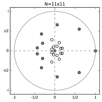
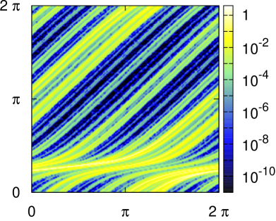
Figure 3: Complex plane (left plot) with exact eigenvalues (open symbols) and approximation by EDMD (full symbols) applied to an analytic deformation of the cat map (12) with $\mu=-0.6-0.55i$. Data obtained from EDMD with $N=11\times 11$ Fourier modes and $M=201\times 201$ nodes on a square lattice. Density plot (right) illustrating the invariant measure for the map (12) for the same parameter values.

Altogether we have compelling evidence that convergence of EDMD points towards an underlying compact operator structure which determines the effective degrees of freedom in a complex dynamical setting.

References

- [1] M. Ahues, A. Largillier, B. Limaye, Spectral Computations for Bounded Operators, Chapman and Hall/CRC, Boca Raton (2001).
- [2] R. Balescu, Kinetic theory of area-preserving maps. Application to the standard map in the diffusive regime, J. Stat. Phys. 98 (2000) 1169–1234.
- [3] O.F. Bandtlow, Resolvent estimates for operators belonging to exponential classes, Integral Equations Operator Theory, 61 (2008) 21–43.
- [4] O.F. Bandtlow, I. Antoniou and Z. Suchanecki, Resonances of dynamical systems and Fredholm-Riesz operators on rigged Hilbert spaces, Comput. Math. Appl. 34 (1997) 95–102.
- [5] O.F. Bandtlow, W. Just and J. Slipantschuk, Spectral structure of transfer operators for expanding circle maps, Ann. Inst. H. Poinc. 34C (2017) 31–43.
- [6] A. Bohm and M. Gadella, Dirac Kets, Gamow Vectors and Gel\cprimefand Triplets. The Rigged Hilbert Space Formulation of Quantum Mechanics, Springer-Verlag, Berlin (1989)
- [7] M. Budišić, R. Mohr and I. Mezić, Applied Koopmanism, Chaos 22 (2012) 047510, 33pp.
- [8] M. Dellnitz, G. Froyland and S. Sertl, On the isolated spectrum of Perron-Frobenius operator, Nonlinearity 13 (2000) 1171–1188.
- [9] M. Dellnitz, O. Junge, On the approximation of complicated dynamical behavior, SIAM J. Numer. Anal., 36 (1999) 491–515.
- [10] N. Dunford and J.T. Schwartz, Linear Operators Part 2: Spectral Theory Wiley Interscience, New York (1963).
- [11] G. Froyland, C. González-Tokman and A. Quas, Detecting isolated spectrum of transfer and Koopman operators with Fourier analytic tools, J. Comput. Dyn. 1 (2014) 249–278.
- [12] I.M. Gel\cprimefand and N.Ya. Vilenkin, Generalized functions, Volume 4, Applications of harmonic analysis, Academic Press, New York (1964)
- [13] D. Giannakis, Data-driven spectral decomposition and forecasting of ergodic dynamical systems, Appl. Comput. Harmon. Anal. (2017 in press), https://doi.org/10.1016/j.acha.2017.09.001
- [14] J. Guckenheimer and P. Holmes, Nonlinear Oscillations, Dynamical Systems, and Bifurcations of Vector Fields, Springer, New York (1986).
- [15] N.G. van Kampen, Elimination of fast variables, Phys. Rep. 124 (1985) 69–160.
- [16] G. Keller, Markov extensions, zeta functions, and Fredholm theory for piecewise invertible dynamical systems, Trans. Amer. Mat. Soc. 314 (1989) 433–497.
- [17] S. Klus, P. Gelß, S. Peitz and C. Schütte, Tensor-based dynamic mode decomposition, Nonlinearity 31 (2018) 3359–3380.
- [18] S. Klus, P. Koltai and C. Schütte, On the numerical approximation of the Perron-Frobenius and Koopman operator, J. Comp. Dyn. 3 (2016) 51–79.
- [19] S. Klus, F. Nüske, P. Koltai, H. Wu, I. Kevrekidis, C. Schütte, F. Noé Data-driven model reduction and transfer operator approximation, J. Nonl. Sci. 28 (2018) 985–1010.
- [20] M. Korda and I. Mezić, On convergence of extended dynamic mode decomposition to the Koopman operator, J. Nonl. Sci. 28 (2018) 687–710.
- [21] N.F.G. Martin, On finite Blaschke products whose restrictions to the unit circle are exact endomorphisms, Bull. Lond. Math. Soc. 15 (1983) 343–348.
- [22] I. Mezić and A. Banaszuk Comparison of systems with complex behavior Phys. D 197 (2004) 101–133.
- [23] S. Nakajima, On quantum theory of transport phenomena, Prog. Theor. Phys. 20 (1958) 948–959.
- [24] I. Prigogine, F. Mayné, C. George and M. De Haan, Microscopic theory of irreversible processes, Proc. Nat. Acad. Sci. USA 74 (1977) 4152–4156.
- [25] E. Pujals and M. Shub, Dynamics of two-dimensional Blaschke products, Ergod. Th. & Dyn. Sys. 20 (2008) 575–585.
- [26] W.C. Saphir and H.H. Hasegawa, Spectral representation of the Bernoulli map, Phys. Lett. A 171 (1992) 317–322.
- [27] P.J. Schmid, Dynamic mode decomposition of numerical and experimental data, J. Fluid Mech. 656 (2010) 5–28.
- [28] J. Slipantschuk, O.F. Bandtlow and W. Just, Analytic expanding circle maps with explicit spectra, Nonlinearity 26 (2013) 3231–3245.
- [29] J. Slipantschuk, O.F. Bandtlow and W. Just, Complete spectral data for analytic Anosov maps of the torus, Nonlinearity 30 (2017) 2667–2686.
- [30] Z. Suchanecki, I. Antoniou, S. Tasaki, and O. F. Bandtlow, Rigged Hilbert spaces for chaotic dynamical systems, J. Math. Phys. 37 (1996) 5837–5847.
- [31] M.O. Williams, I.G. Kevrekidis, C.W. Rowley, A data-driven approximation of the Koopman operator: extending dynamic mode decomposition, J. Nonl. Sci. 25 (2015) 1307–1346.
- [32] R. Zwanzig, Ensemble method in the theory of irreversibility, J. Chem. Phys. 33 (1960) 1338–1341.