Floquet Majorana Corner States Driven by Ferromagnetic Resonance

Floquet Helical Topological Superconductivity Driven by Ferromagnetic Resonance

Floquet Second-Order Topological Superconductor
Driven via Ferromagnetic Resonance

Abstract

We consider a Floquet triple-layer setup composed of a two-dimensional electron gas with spin-orbit interactions, proximity coupled to an $s$-wave superconductor and to a ferromagnet driven at resonance. The ferromagnetic layer generates a time-oscillating Zeeman field which competes with the induced superconducting gap and leads to a topological phase transition. The resulting Floquet states support a second-order topological superconducting phase with a pair of localized zero-energy Floquet Majorana corner states. Moreover, the phase diagram comprises a Floquet helical topological superconductor, hosting a Kramers pair of Majorana edge modes protected by an effective time-reversal symmetry, as well as a gapless Floquet Weyl phase. The topological phases are stable against disorder and parameter variations and are within experimental reach.

 Introduction

Over the last decade topological states of matter [1; 2; 3; 4; 5] have attracted a lot of attention. Recently, particular interest has been raised by higher-order topological insulators and superconductors [6; 7; 8], which host topologically protected gapless modes on their higher-order faces (e.g. corners in $d>1$, hinges in $d>2$, with $d$ being the spatial dimension of the system). However, such systems were studied mostly at the static level [9; 10; 11; 12; 13; 15; 17; 19; 14; 16; 18], with the out-of-equilibrium dynamics [20; 21; 22; 23; 24; 25; 26] rarely addressed. At the same time, Floquet engineering [1; 2; 3; 4], based on applying time-periodic perturbations, has been serving as a powerful tool to generate exotic phases of quantum matter, including topological and Chern insulators [31; 32; 33; 34; 35; 36; 37; 38; 39; 40; 41; 42; 43; 44; 45; 46; 47; 48; 49; 50], as well as non-Abelian states such as Majorana bound states (MBSs) [51; 52; 53; 54; 55; 56; 57; 58; 59]. Such Floquet phases can be generated by time-dependent electromagnetic fields [31; 32; 33; 34; 35; 36; 37; 38; 57; 58]. Strong oscillating electric fields are easy to obtain for this purpose, but the direct coupling to the spin degree of freedom is more challenging, typically achieved only indirectly via strong spin orbit interaction [60; 61]. Hence, finding ways to generate strong oscillating magnetic fields which couple directly to the spin is important. One possible solution consists in using magnetic proximity effects, which, for the static case, have already been widely studied for superconductors [62; 63] and topological insulators [65; 64; 66].

In this work we consider a driven triple-layer setup which allows us to engineer a Floquet higher-order topological superconductor (FHOTS). Its key component is a two-dimensional electron gas (2DEG) with spin-orbit interaction (SOI) sandwiched between an $s$-wave superconductor (SC) and a ferromagnet (FM), as shown in Fig. 1(a). The FM layer is resonantly driven by an external field $\bm{H}(t)$, which results in the generation of an oscillating magnetic field $\bm{B}(t)$, giving rise to strong Zeeman coupling in the 2DEG. The out-of-plane component of $\bm{B}(t)$ competes with the proximity-induced superconducting gap and leads to a topological phase transition in the 2DEG. The topological phase is identified as Floquet helical topological superconductor (FHeTS), characterized by the presence of a Kramers pair of gapless helical Majorana edge modes protected by an effective time-reversal symmetry. A moderate in-plane component of $\bm{B}(t)$ opens a gap in the helical edge modes through a mass term that changes sign at the corners in a rectangular geometry, resulting in Majorana corner states (MCSs) – a distinct feature of the FHOTS. In the regime where the in-plane component of $\bm{B}(t)$ is strong, the system moves into a gapless Weyl phase. The topological phase diagram is robust against moderate local disorder, detuning from resonance, and static magnetic fields.

 Model

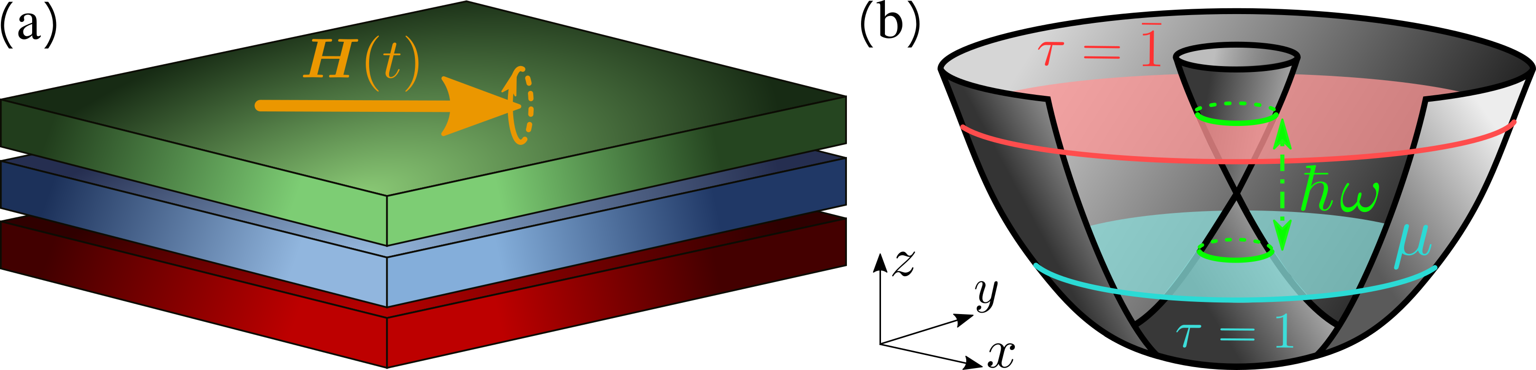
Figure 1: (a) Schematics of the Floquet triple-layer setup consisting of a 2DEG (blue layer) with SOI of strengths $\alpha_{x}$ and $\alpha_{y}$, proximity coupled to an $s$-wave SC (red layer) at the bottom and a FM at the top (green layer) which is resonantly driven by an external time-dependent magnetic field $\bm{H}(t)$ to generate an oscillating magnetic field $\bm{B}(t)=B_{\perp}\cos(\omega t)\bm{e}_{z}+B_{\parallel}\sin(\omega t)\bm{u}_{\parallel}$ in the 2DEG. (b) Band structure of the 2DEG in the isotropic regime $\alpha_{x}=\alpha_{y}$. The chemical potential $\mu$ is fixed below the crossing point of the spin-split bands (indicated by the blue area). The driving frequency $\omega$ is tuned to achieve resonance at the smallest Fermi momentum (represented by the two green circles) between the two Floquet bands labeled by $\tau=\pm 1$.

The triple-layer setup is composed of a 2DEG with strong Rashba and Dresselhaus SOIs, proximity coupled to an $s$-wave SC and a FM, as shown in Fig. 1(a). We assume that the SOI vector is along $z$ direction, which is perpendicular to the $xy$ 2DEG-plane. The SOI coupling strengths $\alpha_{x}=\alpha_{R}+\beta_{D}$ and $\alpha_{y}=\alpha_{R}-\beta_{D}$ are expressed in terms of the Rashba and Dresselhaus SOI coefficients $\alpha_{R}$ and $\beta_{D}$ for a proper choice of the coordinate system [67; 68; 69; 71; 70; 72; 73; 74]. Introducing a creation operator $\psi^{{\dagger}}_{\sigma\bm{k}}$ acting on an electron with momentum $\bm{k}=(k_{x},k_{y})$ and spin component $\sigma$ along the $z$ axis, the corresponding Hamiltonian reads

$$H_{0}=\sum\limits_{\sigma\sigma^{\prime}}\int\textrm{d}\bm{k}\ \psi^{{\dagger}}_{\sigma\bm{k}}\bigg{[}\frac{\hbar^{2}\bm{k}^{2}}{2m}-\mu$$ (1)

$$\hskip 115.0pt-\alpha_{x}k_{x}\sigma_{y}+\alpha_{y}k_{y}\sigma_{x}\bigg{]}_{\sigma\sigma^{\prime}}\!\!\!\psi_{\sigma^{\prime}\bm{k}}\;.$$

Here, $\sigma_{j}$ are the Pauli matrices acting in spin space. The chemical potential $\mu$ is calculated from the crossing point of the two spin-split bands at ${\bm{k}}=0$. In the following, it will be convenient to introduce the SOI energy $E_{\textrm{so}}=\hbar^{2}k_{\textrm{so}}^{2}/(2m)$ and the SOI momentum $k_{\textrm{so}}=m\alpha_{x}/\hbar^{2}$. We note that this Hamiltonian effectively describes a 2D array of coupled Rashba wires if the mass $m$ is also chosen to be anistropic in the $xy$ plane such that $m_{y}\neq m_{x}$  [76; 75; 77; 78; 79; 80; 81; 82; 83; 84; 38; 85; 86].

The proximity effect between the 2DEG and the SC is described by the following Hamiltonian

$$H_{\textrm{sc}}=\frac{\Delta_{\textrm{sc}}}{2}\sum\limits_{\sigma\sigma^{\prime}}\int\textrm{d}\bm{k}\left(\psi^{{\dagger}}_{\sigma\bm{k}}\left[i\sigma_{y}\right]_{\sigma\sigma^{\prime}}\psi^{{\dagger}}_{\sigma^{\prime}(-\bm{k})}+\textrm{H.c.}\right),$$ (2)

where $\Delta_{\textrm{sc}}$ is the induced SC gap. The resulting 2DEG-SC heterostructure is placed in the vicinity of a FM layer, and the setup is subjected to an external magnetic field $\bm{H}(t)$. Under the FM resonance condition (see discussion below), the FM generates an oscillating demagnetizing field which adds up to $\bm{H}(t)$ to produce a total magnetic field $\bm{B}(t)=B_{\perp}\cos(\omega t)\bm{e}_{z}+B_{\parallel}\sin(\omega t)\bm{u}_{\parallel}$ in the 2DEG. Here, $\omega=2\pi/T$ denotes the oscillation frequency and the 2D vector $\bm{u}_{\parallel}=(u_{x},u_{y})$ indicates the orientation of the magnetic field in the $xy$ plane. The FM proximity effect is described by the following Floquet-Zeeman term

$$H_{\textrm{Z}}(t)=2\sum\limits_{\sigma\sigma^{\prime}}\int\textrm{d}\bm{k}\ \psi^{{\dagger}}_{\sigma\bm{k}}\Big{(}t_{\textrm{Z}}^{\perp}\cos(\omega t)[\sigma_{z}]_{\sigma\sigma^{\prime}}$$

$$+ t_{\textrm{Z}}^{\parallel}\sin(\omega t)[\bm{u}_{\parallel}\cdot\bm{\sigma}]_{\sigma\sigma^{\prime}}\Big{)}\psi_{\sigma^{\prime}\bm{k}},$$ (3)

where ${t_{\textrm{Z}}^{\nu}=\mu_{B}g_{\nu}B_{\nu}/2}$ (with $\nu=\parallel,\perp$) are two Floquet-Zeeman amplitudes. The anisotropy in the $g$-factors, which leads to $g_{\parallel}$ and $g_{\perp}$, arises from the quantum confinement and the intrinsic strain of the 2DEG [87; 88; 89].

The resulting time-dependent problem can be solved using the Floquet formalism [1; 2; 3; 4], by writing the quasi-energy operator ${H=H_{0}+H_{\textrm{sc}}+H_{\textrm{Z}}(t)-i\hbar\partial_{t}}$ in the Floquet-Hilbert space generated by $T$-periodic states ${\psi_{l\sigma\bm{k}}=\textrm{exp}(-il\omega t)\psi_{\sigma\bm{k}}}$, $l\in\mathbb{Z}$. In this basis $H$ acquires a simple block-diagonal form, where each block, also referred to as a Floquet band, is composed of the modes with the same index $l$. The static term acts within the same block and receives an additional constant energy shift $\hbar\omega l$, while the oscillating term couples different blocks. We assume that the chemical potential is restricted to $-E_{\textrm{so}}<\mu<0$, so that the frequency $\omega$ can be resonantly tuned to the energy difference between the two spin-split bands. This allows us to treat the oscillating terms at low energies by only taking into account the coupling between the modes at $l=0$, to which we associate a Floquet band index $\tau=1$, and the modes at $l=-1$ with $\tau=\bar{1}$. As a result, in the Nambu basis $\Psi^{{\dagger}}_{\bm{k}}$ = ($\psi^{{\dagger}}_{1\uparrow\bm{k}}$, $\psi^{{\dagger}}_{1\downarrow\bm{k}}$, $\psi^{{\dagger}}_{\bar{1}\uparrow\bm{k}}$, $\psi^{{\dagger}}_{\bar{1}\downarrow\bm{k}}$, $\psi_{1\uparrow-\bm{k}}$, $\psi_{1\downarrow-\bm{k}}$, $\psi_{\bar{1}\uparrow-\bm{k}}$, $\psi_{\bar{1}\downarrow-\bm{k}}$), the total Hamiltonian reads as $H=\int\textrm{d}\bm{k}\ \Psi^{{\dagger}}_{\bm{k}}\mathcal{H}_{\bm{k}}\Psi_{\bm{k}}/2$, with the Hamiltonian density

$$\mathcal{H}_{\bm{k}}=\left[\frac{\hbar^{2}\bm{k}^{2}}{2m}-\mu+\frac{\hbar\omega(\tau_{z}-\tau_{0})}{2}\right]\eta_{z}+\Delta_{\textrm{sc}}\eta_{y}\sigma_{y}+\alpha_{y}k_{y}\sigma_{x}$$

$$-\alpha_{x}k_{x}\eta_{z}\sigma_{y}+t_{\textrm{Z}}^{\perp}\eta_{z}\tau_{x}\sigma_{z}+t_{\textrm{Z}}^{\parallel}\left(u_{x}\tau_{y}\sigma_{x}+u_{y}\eta_{z}\tau_{y}\sigma_{y}\right)$$ (4)

with the Pauli matrices $\tau_{i}$ ($\eta_{i}$) acting in the Floquet (particle-hole) space. In the following, we analyze different topological phases of the system as a function of the parameters appearing in Eq. (II).

 Floquet Helical Topological Superconductor

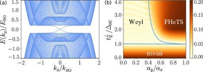
Figure 2: (a) Energy spectrum $E(k_{x})$ in the FHeTS phase with $t_{\textrm{Z}}^{\perp}/\Delta_{\textrm{sc}}=3$ and $\alpha_{x}=\alpha_{y}$. The helical edge modes are localized at the edges. (b) Phase diagram showing the gap to the first excited bulk state (in units of $E_{\textrm{so}}$) as a function of the ratios $\alpha_{y}/\alpha_{x}$ and $t_{\textrm{Z}}^{\perp}/\Delta_{\textrm{sc}}$. Blue lines indicate the phase boundaries. In the isotropic regime, $\alpha_{x}=\alpha_{y}$, the phase transition occurs at the critical point $\Delta_{\textrm{sc}}=t_{\textrm{Z}}^{\perp}$. When $\alpha_{x}\neq\alpha_{y}$, the critical point is transformed into a gapless Weyl phase, and the value $t_{\textrm{Z}}^{\perp}/\Delta_{\textrm{sc}}$ required to reach the FHeTS increases up to the point of strong anisotropy beyond which the FHeTS cannot be reached. Remaining parameters in both simulations are $t_{\textrm{Z}}^{\parallel}=0$, $\Delta_{\textrm{sc}}/E_{\textrm{so}}=0.2$, $k_{\textrm{so}}L_{x}=k_{\textrm{so}}L_{y}=80$, and $\mu=-E_{\textrm{so}}/2$.

In order to determine the phase diagram of our model, we first consider the effect of the out-of-plane component of $\bm{B}(t)$ by imposing $t_{\textrm{Z}}^{\parallel}=0$ in Eq. (II). In the isotropic regime with $\alpha_{x}=\alpha_{y}$, the Fermi surface is composed of two concentric circles and the problem depends only on the magnitude of the momentum $|\bm{k}|$, as shown in Fig. 1(b). The resonance condition for the frequency $\omega$ is satisfied along the entire circle with the smallest Fermi momentum (see the Supplemental Material (SM) [90] for more details). The Hamiltonian is linearized close to the Fermi surface and provides the eigenenergies $E_{1}^{2}=(\hbar v_{F}\delta k)^{2}+\Delta_{\textrm{sc}}^{2}$ and $E_{2,\pm}^{2}=(\hbar v_{F}\delta k)^{2}+(t_{\textrm{Z}}^{\perp}\pm\Delta_{\textrm{sc}})^{2}$, with $v_{F}=\alpha_{x}/\hbar$ the Fermi velocity and $\delta k$ the radial distance from the Fermi surface. The phase diagram consists of two gapped phases separated by the gapless line $\Delta_{\textrm{sc}}=t_{\textrm{Z}}^{\perp}$. The topologically trivial (topological) phase is identified with the regime $\Delta_{\textrm{sc}}>t_{\textrm{Z}}^{\perp}$ ($\Delta_{\textrm{sc}}<t_{\textrm{Z}}^{\perp}$). For $t_{\textrm{Z}}^{\parallel}=0$, the system is characterized by an emerging effective time-reversal symmetry $T_{\textrm{eff}}=-i\tau_{z}\sigma_{y}\mathcal{K}$, a particle-hole symmetry $P=\eta_{x}\mathcal{K}$, and a chiral symmetry $U_{C}=PT_{\textrm{eff}}$, with $\mathcal{K}$ the complex-conjugation operator. Thus, the system belongs to the DIII symmetry class with $\mathbb{Z}_{2}$ topological invariant.

The topological phase, denoted as FHeTS, hosts gapless boundary modes – a Kramers pair of Floquet Majorana fermions $\ket{\Phi_{\pm}}$, obeying $P\ket{\Phi_{\pm}}=\ket{\Phi_{\pm}}$ and $T_{\textrm{eff}}\ket{\Phi_{\pm}}=\pm\ket{\Phi_{\mp}}$. The Kramers partners propagate in opposite directions along the same edge, forming a pair of helical modes protected by the effective time-reversal and particle-hole symmetries. We have verified the presence of these modes numerically in the discretized version of the model (see the SM [90]) defined on a rectangular lattice of size $L_{x}\times L_{y}$ with periodic boundary conditions along $x$, as shown in Fig. 2(a).

If the rotation symmetry is broken ($\alpha_{x}\neq\alpha_{y}$), the resonance condition can be satisfied only along a particular direction in momentum space, resulting in an off-set $\delta\omega$ in the resonance condition almost everywhere except at a few points on the Fermi surface. While a small $\delta\omega$ in the weak anisotropy regime hardly affects the phase diagram and can be compensated by increasing $t_{\textrm{Z}}^{\perp}$, strong anisotropy effects are more drastic. In Fig. 2(b), we calculate numerically the energy of the lowest bulk state as a function of the ratios $\alpha_{y}/\alpha_{x}$ and $t_{\textrm{Z}}^{\perp}/\Delta_{\textrm{sc}}$. We see that the critical point $\Delta_{\textrm{sc}}=t_{\textrm{Z}}^{\perp}$ transforms into a gapless Weyl phase at a finite value of anisotropy $(\alpha_{y}-\alpha_{x})/\alpha_{x}$. This gapless regime is characterized by a semi-metal energy structure with four Weyl cones. The nodes of the Weyl cones appear first on the Fermi surface and move further in the reciprocal space, when the parameters $t_{\textrm{Z}}^{\perp}/\Delta_{\textrm{sc}}$ and $\alpha_{y}/\alpha_{x}$ are modified. We also note that if we decrease the ratio $t_{\textrm{Z}}^{\perp}/\Delta_{\textrm{sc}}$ up to a point of reaching the phase transition to the trivial phase, the low energy physics becomes insensitive to the anisotropy.

 Floquet Majorana corner states

Next, we analyze the effect of an oscillating in-plane magnetic field that breaks the effective time-reversal symmetry $T_{\textrm{eff}}$ and, thus, gaps out the helical edge modes of the FHeTS. Nevertheless, the system remains topologically non-trivial as it now hosts a set of zero-energy MCSs, characteristic for the FHOTS phase [91]. The presence of such MCSs is uncovered by focussing on the low-energy degrees of freedom expressed in terms of the Majorana edge modes $\ket{\Phi_{\pm}}$. The in-plane Zeeman field $B_{\parallel}$ couples the two helical modes, leading to the following low-energy Hamiltonian density:

$$\mathcal{H}_{\textrm{edge}}=\hbar v^{e}_{F}|\bm{k}|\rho_{z}+\tilde{t}^{\parallel}_{\textrm{Z}}\rho_{y}\;,$$ (5)

where the Pauli matrices $\rho_{i}$ act in the space of $\ket{\Phi_{\pm}}$, $v^{e}_{F}$ is the velocity of the helical edge modes, and ${\tilde{t}^{\parallel}_{\textrm{Z}}=t^{\parallel}_{\textrm{Z}}\mathfrak{Im}\braket{\Phi_{-}}{u_{x}\tau_{y}\sigma_{x}+u_{y}\eta_{z}\tau_{y}\sigma_{y}}{\Phi_{+}}}$ is the ‘mass term’. Thus, our system is described by the well-known Jackiw-Rebbi model [7; 8].

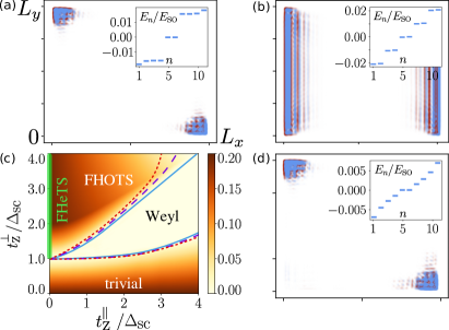
Figure 3: (a,b,d) Probability density of the lowest energy state in the FHOTS phase for $t^{\perp}_{\textrm{Z}}/\Delta_{\textrm{sc}}=3$, $t^{\parallel}_{\textrm{Z}}/\Delta_{\textrm{sc}}=2.5$, and $\alpha_{x}=\alpha_{y}$. The inset shows the 10 lowest eigenenergies. (a) For ${\bm{u}_{\parallel}=(1,1)/\sqrt{2}}$, the in-plane Zeeman field $B_{\parallel}$ opens gaps in all edge modes such that zero-energy MCSs emerge at two opposite corners. (b) The vector $\bm{u}_{\parallel}=(0,1)$ is parallel to the edges along which the system stays gapless. (c) Phase diagram showing the bulk gap (color coded in units of $E_{\textrm{so}}$) as a function of the ratios $t^{\perp}_{\textrm{Z}}/\Delta_{\textrm{sc}}$ and $t^{\parallel}_{\textrm{Z}}/\Delta_{\textrm{sc}}$ with ${\bm{u}_{\parallel}=(1,1)/\sqrt{2}}$. The critical point $\Delta_{\textrm{sc}}=t^{\perp}_{\textrm{Z}}$ at $t^{\parallel}_{\textrm{Z}}=0$ merges into a gapless Weyl phase at finite $t^{\parallel}_{\textrm{Z}}$. As a result, higher value of $t^{\perp}_{\textrm{Z}}/\Delta_{\textrm{sc}}$ are required to reach the topological phase. The various phase boundaries correspond to $\alpha_{y}/\alpha_{x}=0.8$ (red dotted), $0.9$ (purple dashed), and $1.0$ (blue solid). (d) The MCSs are stable against moderate external perturbations and disorder: $\delta\omega=\sqrt{3}S_{\mu}=\Delta_{\textrm{Z}}=0.10E_{\textrm{so}}$. Rest of parameters are the same as in Fig. 2.

From the symmetry of the modes $\ket{\Phi_{\pm}}$, we deduce that the value of the mass term $\tilde{t}^{\parallel}_{\textrm{Z}}$ only depends on the component of the in-plane field $B_{\parallel}$ which is perpendicular to the corresponding edge in a rectangular geometry (see the SM [90]). Generally, the sign of $\tilde{t}^{\parallel}_{\textrm{Z}}$ is opposite on two parallel edges at $x=0$ ($y=0$) and $x=L_{x}$ ($y=L_{y}$). Hence, $\tilde{t}^{\parallel}_{\textrm{Z}}$ has to change its sign at two opposite corners of the 2DEG, leading to the emergence of domain walls at these corners that host zero-energy MCSs, see Fig. 3(a). In the special case when $\bm{u}_{\parallel}$ is parallel to one of the edges, the corresponding edge modes stay gapless, see Fig. 3(b).

The simple boundary description in terms of the Jackiw-Rebbi model is expected to work in the regime where the amplitude of the in-plane magnetic field is small. In order to construct the full phase diagram, we calculated numerically the gap to the first excited bulk state as a function of the ratios $t^{\perp}_{\textrm{Z}}/\Delta_{\textrm{sc}}$ and $t^{\parallel}_{\textrm{Z}}/\Delta_{\textrm{sc}}$, see Fig. 3(c). The FHOTS phase emerges from the FHeTS phase at non-zero $t^{\parallel}_{\textrm{Z}}$. However, if $t^{\parallel}_{\textrm{Z}}$ is large, the system enters into the gapless Weyl phase. To observe MCSs, the Floquet-Zeeman field perpendicular to the 2DEG plane should dominate such that the condition $t_{\textrm{Z}}^{\parallel}<t_{\textrm{Z}}^{\perp}$ is fulfilled. All the results remain qualitatively the same for a weak anisotropy ($\alpha_{x}\neq\alpha_{y}$), which shifts the topological phase transition line only slightly.

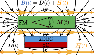
Figure 4: Setup of the FM layer to generate the desired oscillating magnetic field in the 2DEG. The 2DEG-SC heterostructure is placed in the vicinity of the FM. The system is subjected to an external magnetic field $\bm{H}(t)=\bm{H}_{0}+\bm{h}(t)$ (yellow lines) generating FM resonance (shown not to scale). This induces the precession of the FM magnetization $\bm{M}(t)$ (black lines inside the FM) and demagnetizing field $\bm{D}(t)$ (black lines outside of the FM). Close to the surface of the FM layer, the static components of $\bm{D}(t)$ and $\bm{H}(t)$ cancel out, so that the dynamics of the total field $\bm{B}(t)=\bm{H}(t)+\bm{D}(t)$ in the 2DEG layer is close to a full $360^{\circ}$ rotation.

 Experimental feasibility

Next, we discuss the stability of our setup. We check numerically that the topological phases are robust against an off-set $\delta\omega$ in the resonance frequency $\omega$. Similarly, we check the stability with respect to an on-site disorder by adding a fluctuating chemical potential randomly chosen from a uniform distribution with standard deviation $S_{\mu}$ and with respect to a static magnetic field by adding a Zeeman term with strength $\Delta_{\textrm{Z}}$ directed both in-plane and out-of-plane. The result of the calculations is shown in Fig. 3(d). The topological phases are stable against the perturbations of a strength comparable to the gap. The effect of the out-of-plane component of the static magnetic field is also less important: the MCSs can be observed even for $\Delta_{\textrm{Z}}\sim t^{\perp}_{\textrm{Z}}$ and disappear only when the static term becomes stronger.

In experiments, the proximity induced SC gap $\Delta_{\textrm{sc}}$ is expected to be of the order of $0.05$ meV, depending on the properties of the SC and the strength of the coupling between the SC and the 2DEG [94; 95; 96]. As shown in this work, the strength of the Floquet-Zeeman amplitude $t_{\textrm{Z}}^{\perp}$ should exceed $\Delta_{\textrm{sc}}$ to reach the topological regimes. Hence, assuming that the 2DEG material has an electron $g$-factor $g_{\perp}=15$, the amplitude of the magnetic field $B_{\perp}$ should be of the order of $0.1$ T. At the same time, the static component of the magnetic field should be smaller than the dynamic one and the oscillation frequency $\omega$ should be in the GHz range. The FM layer in the setup is proposed to generate the required Zeeman fields as follows. Applying an external magnetic field $\bm{H}(t)=\bm{H}_{0}+\bm{h}(t)$ with $|\bm{h}(t)|\ll|\bm{H}_{0}|$ and $\bm{h}(t)\perp\bm{H}_{0}$ under FM resonance condition induces a precession of the FM magnetization $\bm{M}(t)$ [11; 12]. The precession cone of $\bm{M}(t)$ depends on the angle between the FM easy axis and $\bm{H}_{0}$, while the resonance frequency is determined by the magnitude $|\bm{H}_{0}|$. Outside of the FM, the total field $\bm{B}(t)$ is equal to the sum of the external field $\bm{H}(t)$ and an oscillating demagnetizing field $\bm{D}(t)$, see Fig. 4. Hence, by carefully choosing the system geometry, the static component of $\bm{B}(t)$ could be adjusted close to zero over a large region of space in the proximity of the FM surface including the 2DEG. The amplitude of the remaining oscillating component overcomes the threshold of $0.1$ T inside the 2DEG, as we have confirmed by micromagnetic simulations (see the SM [90]). Promising candidates for such FMs are e.g. EuS [64], GdN [65], and YiG [66].

Alternatively, the fast switching or the sustained oscillation of the FM magnetization has already been achieved experimentally by shining optical light on a FM (via an all-optical magnetization reversal) [99; 100; 101], by applying piezostrain [102; 103] or by injecting a spin-polarized current (via a spin-orbit torque) [104; 105; 106; 107; 108]. This domain of research is currently under an active exploration because of its crucial role in the implementation of magnetic memory and logic devices. We also note that in our setup, the magnetic field in the 2DEG can originate from both the FM demagnetizing field at a moderate range and from the exchange interactions at atomic distances.

 Conclusions

We have considered a Floquet triple-layer setup of a 2DEG proximity coupled to a SC and a FM. Under resonant drive the FM induces an oscillating Zeeman field in the 2DEG. The out-of-plane component of the magnetic field competes with the proximity induced SC gap and leads to the emergence of the FHeTS hosting an effective Kramers pair of gapless helical edge modes. Moreover, the in-plane component of the magnetic field enters into the low-energy description corresponding to the effective Jackiw-Rebbi model as a mass term and opens a gap in the edge mode spectrum. Change in the sign of the mass term, which inevitably occurs at two opposite corners of the system in a rectangular geometry, leads to the emergence of Floquet MCSs. We argued that the proposed setup is within experimental reach combining available magnetic, semiconducting, and superconducting materials.

S1.  Topological criterion in the isotropic limit

In the isotropic limit, $\alpha_{x}=\alpha_{y}$, when the in-plane component of the oscillating magnetic field is zero, $t_{\textrm{Z}}^{\parallel}=0$, the system described by the Hamiltonian given in Eq. (4) has a continuous rotation symmetry in the $xy$ plane. The corresponding symmetry operator reads $U^{\textrm{rot}}_{J_{z}}(\theta)=\exp\left(-i\theta\eta_{z}J_{z}/\hbar\right)$, with $\theta$ being the rotation angle and $J_{z}$ the $z$ component of the orbital angular momentum operator. Thus, the energy structure depends only on the absolute value of the momentum $|\bm{k}|=\sqrt{k_{x}^{2}+k_{y}^{2}}$ and can be calculated along a particular direction in the $xy$ plane. For simplicity we perform the calculations along the axis $k_{y}=0$ [see Fig. S1]. This results in the following Hamiltonian density

$$\mathcal{H}_{\bm{k}}(k_{y}=0)=\left(\frac{\hbar^{2}k_{x}^{2}}{2m}-\mu\right)\eta_{z}-\alpha_{x}k_{x}\eta_{z}\sigma_{y}+\Delta_{\textrm{sc}}\eta_{y}\sigma_{y}+t_{\textrm{Z}}^{\perp}\eta_{z}\tau_{x}\sigma_{z}+\hbar\omega\eta_{z}\left(\frac{\tau_{z}-\tau_{0}}{2}\right)\;.$$ (S1)

Here, similar to the main text, we work in the Nambu basis $\Psi^{{\dagger}}_{\bm{k}}$ = ($\psi^{{\dagger}}_{1\uparrow\bm{k}}$, $\psi^{{\dagger}}_{1\downarrow\bm{k}}$, $\psi^{{\dagger}}_{\bar{1}\uparrow\bm{k}}$, $\psi^{{\dagger}}_{\bar{1}\downarrow\bm{k}}$, $\psi_{1\uparrow-\bm{k}}$, $\psi_{1\downarrow-\bm{k}}$, $\psi_{\bar{1}\uparrow-\bm{k}}$, $\psi_{\bar{1}\downarrow-\bm{k}}$). We define by $\eta_{i}$ the Pauli matrices (the $2\times 2$ identity matrix for $i=0$) acting on the particle-hole space, $\tau_{i}$ – on the Floquet space, $\sigma_{i}$ – on the space associated with the two spin components in the $z$ direction. The total Hamiltonian acts in the corresponding tensor-product space and for notational simplicity we suppress the explicit writing of the tensor product sign and the identity matrices. The system is characterized by an effective time-reversal symmetry $T_{\textrm{eff}}=U_{T}\mathcal{K}=-i\tau_{z}\sigma_{y}\mathcal{K}$ with $U_{T}^{{\dagger}}\mathcal{H}_{\bm{k}}U_{T}=\mathcal{H}^{*}_{-\bm{k}}$, a particle-hole symmetry $P=U_{P}\mathcal{K}=\eta_{x}\mathcal{K}$ with $U_{P}^{{\dagger}}\mathcal{H}_{\bm{k}}U_{P}=-\mathcal{H}^{*}_{-\bm{k}}$, and a chiral symmetry $U_{C}=PT_{\textrm{eff}}=-i\eta_{x}\tau_{z}\sigma_{y}$ with $U_{C}^{{\dagger}}\mathcal{H}_{\bm{k}}U_{C}=-\mathcal{H}_{\bm{k}}$. From this we deduce that the system belongs to the DIII symmetry class, characterized by $\mathbb{Z}_{2}$ topological invariants, and has two distinct topological phases.

In the following, it will be convenient to change to the spin basis with quantization axis along the $y$ direction, using the unitary rotation in the $yz$ plane described by the operator $U^{\textrm{rot}}_{\sigma_{x}}=\exp\left(-i\pi\eta_{z}\sigma_{x}/4\right)$. This transformation satisfies $\tilde{\Psi}_{\bm{k}}=U^{\textrm{rot}}_{\sigma_{x}}\Psi_{\bm{k}}$ and $\tilde{\mathcal{H}}_{\bm{k}}=U^{\textrm{rot}}_{\sigma_{x}}\mathcal{H}_{\bm{k}}{U^{\textrm{rot}}_{\sigma_{x}}}^{{\dagger}}$, with

$$\tilde{\mathcal{H}}_{\bm{k}}(k_{y}=0)=\left(\frac{\hbar^{2}k_{x}^{2}}{2m}-\mu\right)\eta_{z}-\alpha_{x}k_{x}\sigma_{z}+\Delta_{\textrm{sc}}\eta_{y}\sigma_{y}+t_{\textrm{Z}}^{\perp}\tau_{x}\sigma_{y}+\hbar\omega\eta_{z}\left(\frac{\tau_{z}-\tau_{0}}{2}\right)\;.$$ (S2)

In the new spin basis the Rashba SOI term acts on the spin component along the $z$ axis and we denote by $\sigma=1,\bar{1}$ its two possible orientations. In order to achieve the resonance condition, we first fix the chemical potential $\mu$ to be smaller in absolute value than the SOI energy, $-E_{\textrm{so}}<\mu<0$. For instance, we restrict the discussion to the Floquet band $\tau=1$ only. As a result of the Rashba SOI, which lifts the spin degeneracy, there are four Fermi momenta

$$k^{F}_{1\sigma\pm}=\sigma k_{\textrm{so}}\pm k_{\mu},\quad\text{with}\ k_{\mu}=\sqrt{\frac{2m\left(E_{\textrm{so}}+\mu\right)}{\hbar^{2}}},\ k_{\textrm{so}}=\frac{m\alpha_{x}}{\hbar^{2}},\ \text{and}\ E_{\textrm{so}}=\frac{\hbar^{2}k_{\textrm{so}}^{2}}{2m}\;.$$ (S3)

The resonance condition is fixed at the momentum $k_{\textrm{res}}=k^{F}_{11-}$, where the spin-split band $\sigma=1$ crosses the chemical potential $\mu$, as shown in Fig. S1. The resonance frequency is tuned to the energy difference between the two spin-split bands. Since the energy of the band $\sigma=1$ at $k_{\textrm{res}}$ is zero, $\hbar\omega$ is simply equal to the energy of the band $\sigma=\bar{1}$, which can be written as

$$\hbar\omega=\frac{\hbar^{2}\left(k_{\textrm{res}}+k_{\textrm{so}}\right)^{2}}{2m}-\frac{\hbar^{2}\left(k_{\textrm{res}}-k_{\textrm{so}}\right)^{2}}{2m}=4E_{\textrm{so}}\left(1-\sqrt{\frac{E_{\textrm{so}}+\mu}{E_{\textrm{so}}}}\right)\;.$$ (S4)

According to the Floquet formalism [1, 2, 3, 4], the second Floquet band $\tau=\bar{1}$ is shifted in energy with respect to the first band $\tau=1$ by an energy $-\hbar\omega$. Hence, it crosses the chemical potential $\mu$ at four momenta

$$k^{F}_{\bar{1}\sigma\pm}=\sigma k_{\textrm{so}}\pm(2k_{\textrm{so}}-k_{\mu})\;.$$ (S5)

When $\omega$ is at resonance, the following identities hold true: $k^{F}_{\bar{1}\bar{1}+}=k^{F}_{11-}=k_{\textrm{res}}$ and $k^{F}_{\bar{1}1-}=k^{F}_{1\bar{1}+}=-k_{\textrm{res}}$.

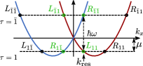
Figure S1: The band structure of the 2DEG with SOI in the isotropic regime $\alpha_{x}=\alpha_{y}$ expressed as a function of $k_{x}$ at $k_{y}=0$ and chemical potential $\mu$ (dashed line at bottom). The frequency $\omega$ of a periodic drive is chosen resonantly such that the two Floquet bands (corresponding to $\tau=1,\bar{1}$) have the same smallest Fermi momentum $k_{\textrm{res}}$ (indicated by green circles) for the two spin-split bands (represented by the blue and red colors). Operators $R_{\tau\sigma}$ and $L_{\tau\sigma}$ correspond to the slowly varying left and right movers. The symbols colored in green indicate the operators involved in the resonant process at $k_{\textrm{res}}$.

To see the effect of $t^{\perp}_{\textrm{Z}}$ and $\Delta_{\textrm{sc}}$ analytically, we linearize the spectrum around the Fermi momenta $k^{F}_{\tau\sigma\pm}$ and represent the original operators in terms of slowly varying left and right moving fields [5, 6] using the following relations

$$\tilde{\psi}_{1\sigma}(x) =\tilde{R}_{1\sigma}(x)e^{-ik^{F}_{1\sigma+}x}+\tilde{L}_{1\sigma}(x)e^{-ik^{F}_{1\sigma-}x}\;,$$

$$\tilde{\psi}_{\bar{1}\sigma}(x) =\tilde{R}_{\bar{1}\sigma}(x)e^{-ik^{F}_{\bar{1}\sigma+}x}+\tilde{L}_{\bar{1}\sigma}(x)e^{-ik^{F}_{\bar{1}\sigma-}x}\;.$$ (S6)

In the basis associated with the slowly varying fields, the Hamiltonian density becomes

$$\tilde{\mathcal{H}}_{\bm{k}}(k_{y}=0)=\hbar v_{F}\delta k\rho_{z}+\Delta_{\textrm{sc}}\rho_{x}\eta_{y}\sigma_{y}+\frac{t_{\textrm{Z}}^{\perp}}{2}\tau_{x}\left(\rho_{x}\sigma_{y}-\rho_{y}\sigma_{x}\right)\;.$$ (S7)

Here $v_{F}=\alpha_{x}/\hbar$ is the Fermi velocity assumed to be equal for both Floquet bands, $\delta k=k_{x}-k^{F}_{\tau\sigma\pm}$ is the distance from the Fermi momenta $k^{F}_{\tau\sigma\pm}$, and the Pauli matrices $\rho_{i}$ act on the space of left and right movers. The bulk spectrum of the linearized problem is given by

$$E_{1}^{2}=(\hbar v_{F}\delta k)^{2}+\Delta_{\textrm{sc}}^{2},\quad E_{2,\pm}^{2}=(\hbar v_{F}\delta k)^{2}+(t_{\textrm{Z}}^{\perp}\pm\Delta_{\textrm{sc}})^{2}\;.$$ (S8)

Both the Floquet-Zeeman and the superconducting terms induce an opening of the gap at the Fermi momenta $\pm k_{\textrm{res}}$, which leads to a competition between the two terms. In contrast, the gap at the remaining Fermi momenta is opened only by the superconducting term. When the Floquet amplitude $t_{\textrm{Z}}^{\perp}$ becomes of the same strength as the superconducting pairing amplitude $\Delta_{\textrm{sc}}$, we observe the closing of the gap, indicating a topological phase transition. When $\Delta_{\textrm{sc}}>t_{\textrm{Z}}^{\perp}$ the system is in the topologically trivial phase, while in the regime $\Delta_{\textrm{sc}}<t_{\textrm{Z}}^{\perp}$ it hosts a Kramers pair of helical Majorana edge modes, connected one to another via $T_{\textrm{eff}}$, as shown in Fig. 2(a) of the main text.

S2.  Boundary description of the FHeTS and FHOTS phases

In order to better understand the two topological phases emerging in our model, we study its low-energy behavior with focus on the boundary of the system. For simplicity, we again consider only the isotropic case $\alpha_{x}=\alpha_{y}$ here. We start with the FHeTS phase which is characterized by the presence of helical gapless edge modes, as shown in Fig. 2(a). We consider a strip geometry with periodic boundary conditions along $y$ and open boundary conditions along $x$. In such a geometry two pairs of helical gapless modes have to be localized at the two edges at $x=0$ and $x=L_{x}$. As a result of the interplay between the time-reversal symmetry $T_{\textrm{eff}}$ and the particle-hole symmetry $P$, the energy of these states at $k_{y}=0$ has to be equal to zero. Hence, in order to find such states, we look for a zero-energy solution of the real-space version of the Hamiltonian (S2). For convenience, we keep working in the spin basis with quantization axis along $y$ direction. We identify the momentum $k_{x}$ with the spatial derivative $-i\hbar\partial_{x}$ and linearize the Hamiltonian around the momenta $k^{F}_{\tau\sigma\pm}$ in the basis of slowly varying fields of Eq.(S1), which leads to

$$\tilde{\mathcal{H}}(x,k_{y}=0)=-i\hbar v_{F}\rho_{z}\partial_{x}+\Delta_{\textrm{sc}}\rho_{x}\eta_{y}\sigma_{y}+\frac{t_{\textrm{Z}}^{\perp}}{2}\tau_{x}\left(\rho_{x}\sigma_{y}-\rho_{y}\sigma_{x}\right)\;.$$ (S9)

We now solve the equation $\tilde{\mathcal{H}}(x,k_{y}=0)\ket{\tilde{\Phi}_{\pm}}=0$, assuming that $\ket{\tilde{\Phi}_{\pm}}$ are two states connected to each other through the effective time-reversal transformation $T_{\textrm{eff}}\ket{\tilde{\Phi}_{\pm}}=\pm\ket{\tilde{\Phi}_{\mp}}$. They can be explicitly written as $\ket{\tilde{\Phi}_{\pm}}=\sum_{x,j}\tilde{\Phi}^{j}_{\pm}(x)\ket{x,j}$ in the orthonormal basis of spatially localized states $\ket{x,j}$ with an orbital (Nambu) index $j$. We are particularly interested in solutions of the form $P\ket{\tilde{\Phi}_{\pm}}=\ket{\tilde{\Phi}_{\pm}}$ associated with self-adjoint Majorana operators. We also focus on the edge at $x=0$, which requires imposing vanishing boundary conditions $\tilde{\Phi}^{j}_{\pm}(x=0)=0$ for all $j$. We find that such solutions exist only in the topological phase $\Delta_{\textrm{sc}}<t_{\textrm{Z}}^{\perp}$ and are expressed as follows (suppressing normalization constants):

$$\tilde{\Phi}_{+}(x)=\Big{(}f_{1},g_{1},f_{\bar{1}},g_{\bar{1}},f^{*}_{1},g^{*}_{1},f^{*}_{\bar{1}},g^{*}_{\bar{1}}\Big{)}^{T},$$

$$\tilde{\Phi}_{-}(x)=\Big{(}-g_{1}^{*},f_{1}^{*},g_{\bar{1}}^{*},-f_{\bar{1}}^{*},-g_{1},f_{1},g_{\bar{1}},-f_{\bar{1}}\Big{)}^{T},$$

$$f_{\tau}(x)=-ig_{\tau}^{*}(x)=e^{-ixk^{F}_{\tau\sigma+}}e^{-x/\xi}-e^{-ixk^{F}_{\tau\sigma-}}e^{-x/\xi_{-}}\;.$$ (S10)

Here, $\xi=\hbar v^{\prime}_{F}/\Delta_{\textrm{sc}}$ and $\xi_{-}=\hbar v^{\prime}_{F}/\left(t_{\textrm{Z}}^{\perp}-\Delta_{\textrm{sc}}\right)$ are two correlation lengths. Functions $f_{\tau}$ and $g_{\tau}$ are related to each other as a result of the presence of an additional spatial unitary symmetry in the system. This symmetry reads as $U_{\textrm{MF}}=\eta_{y}\sigma_{x}$, with ${U_{\textrm{MF}}\tilde{\mathcal{H}}_{\bm{k}}(k_{y}=0){U_{\textrm{MF}}}^{{\dagger}}=-\tilde{\mathcal{H}}_{\bm{k}}(k_{y}=0)}$ and $U_{\textrm{MF}}\ket{\tilde{\Phi}_{\pm}}=\ket{\tilde{\Phi}_{\pm}}$. When $k_{y}$ is non-zero, it also maps the $y$ component of the momentum, i.e., $k_{y}\rightarrow-k_{y}$, effectively exchanging the two helical components of the gapless edge mode.

In the second part of this section we show how the modulated in-plane magnetic field with an amplitude $t_{\textrm{Z}}^{\perp}$ couples the two helical Majorana fermion edge modes $\ket{\tilde{\Phi}_{\pm}}$ living on the edge $x=0$ and leads to the emergence of the FHOTS phase hosting MCSs. First, we write down the corresponding Hamiltonian density in the $y$-spin basis as

$$\tilde{\mathcal{H}}_{\textrm{Z}}^{\parallel}=t_{\textrm{Z}}^{\parallel}\left(u_{x}\tau_{y}\sigma_{x}+u_{y}\tau_{y}\sigma_{z}\right)={U^{\textrm{rot}}_{\sigma_{x}}}^{{\dagger}}\mathcal{H}_{\textrm{Z}}^{\parallel}U^{\textrm{rot}}_{\sigma_{x}}={U^{\textrm{rot}}_{\sigma_{x}}}^{{\dagger}}\left[t_{\textrm{Z}}^{\parallel}\left(u_{x}\tau_{y}\sigma_{x}+u_{y}\eta_{z}\tau_{y}\sigma_{y}\right)\right]U^{\textrm{rot}}_{\sigma_{x}}\;.$$ (S11)

Using the particle-hole symmetry $P$, we deduce that all the diagonal components of $\tilde{\mathcal{H}}^{\parallel}_{\textrm{Z}}$ in this basis of states $\ket{\tilde{\Phi}_{\pm}}$ are exactly zero:

$$\braket{\tilde{\Phi}_{\pm}}{\tau_{y}\sigma_{x}}{\tilde{\Phi}_{\pm}} =\braket{\tilde{\Phi}_{\pm}}{P\tau_{y}\sigma_{x}P}{\tilde{\Phi}_{\pm}}=-\braket{\tilde{\Phi}_{\pm}}{\tau_{y}\sigma_{x}}{\tilde{\Phi}_{\pm}}=0\;,$$

$$\braket{\tilde{\Phi}_{\pm}}{\tau_{y}\sigma_{z}}{\tilde{\Phi}_{\pm}} =\braket{\tilde{\Phi}_{\pm}}{P\tau_{y}\sigma_{z}P}{\tilde{\Phi}_{\pm}}=-\braket{\tilde{\Phi}_{\pm}}{\tau_{y}\sigma_{z}}{\tilde{\Phi}_{\pm}}=0\;.$$ (S12)

Employing the effective time-reversal symmetry $T_{\textrm{eff}}$, we also find that all the off-diagonal terms are purely imaginary:

$$\braket{\tilde{\Phi}_{-}}{\tau_{y}\sigma_{x}}{\tilde{\Phi}_{+}} =-\braket{\tilde{\Phi}_{+}}{T_{\textrm{eff}}\tau_{y}\sigma_{x}T_{\textrm{eff}}}{\tilde{\Phi}_{-}}=-\braket{\tilde{\Phi}_{+}}{\tau_{y}\sigma_{x}}{\tilde{\Phi}_{-}}=-\braket{\tilde{\Phi}_{-}}{\tau_{y}\sigma_{x}}{\tilde{\Phi}_{+}}^{*}\;,$$

$$\braket{\tilde{\Phi}_{-}}{\tau_{y}\sigma_{z}}{\tilde{\Phi}_{+}} =-\braket{\tilde{\Phi}_{+}}{T_{\textrm{eff}}\tau_{y}\sigma_{z}T_{\textrm{eff}}}{\tilde{\Phi}_{-}}=-\braket{\tilde{\Phi}_{+}}{\tau_{y}\sigma_{z}}{\tilde{\Phi}_{-}}=-\braket{\tilde{\Phi}_{-}}{\tau_{y}\sigma_{z}}{\tilde{\Phi}_{+}}^{*}\;.$$ (S13)

This allows us to rewrite the term $\tilde{\mathcal{H}}_{\textrm{Z}}^{\parallel}$ to the zeroth order in perturbation theory as $\tilde{\mathcal{H}}_{\textrm{Z}}^{\parallel}=\tilde{t}_{\textrm{Z}}^{\parallel}\rho_{y}$, with the Pauli matrix $\rho_{i}$ acting in the space of $\ket{\tilde{\Phi}_{\pm}}$ and $\tilde{t}_{\textrm{Z}}^{\parallel}=t_{\textrm{Z}}^{\parallel}\mathfrak{Im}\braket{\tilde{\Phi}_{-}}{u_{x}\tau_{y}\sigma_{x}+u_{y}\tau_{y}\sigma_{z}}{\tilde{\Phi}_{+}}$. Moreover, using the spatial unitary symmetry $U_{\textrm{MF}}$, we find that

$$\braket{\tilde{\Phi}_{-}}{\tau_{y}\sigma_{z}}{\tilde{\Phi}_{+}} =-\braket{\tilde{\Phi}_{-}}{\tau_{y}\sigma_{z}PT_{\textrm{eff}}}{\tilde{\Phi}_{-}}=i\braket{\tilde{\Phi}_{-}}{\eta_{x}\tau_{y}\tau_{z}\sigma_{z}\sigma_{y}}{\tilde{\Phi}_{-}}=i\braket{\tilde{\Phi}_{-}}{\eta_{x}\tau_{x}\sigma_{x}}{\tilde{\Phi}_{-}}$$

$$=i\braket{\tilde{\Phi}_{-}}{U_{\textrm{MF}}^{{\dagger}}\eta_{x}\tau_{x}\sigma_{x}{U_{\textrm{MF}}}}{\tilde{\Phi}_{-}}=-i\braket{\tilde{\Phi}_{-}}{\eta_{x}\tau_{x}\sigma_{x}}{\tilde{\Phi}_{-}}=0\;.$$ (S14)

Hence, the $y$ component of the magnetic field does not contribute to the emergence of the mass term $\tilde{t}_{\textrm{Z}}^{\parallel}$ on the edge $x=0$. As a result, the mass term can be simply expressed using the functions $f_{\eta}$ and $g_{\eta}$ as

$$\tilde{t}_{\textrm{Z}}^{\parallel}=2t_{\textrm{Z}}^{\parallel}u_{x}\int_{0}^{\infty}dx\ \mathfrak{Im}\left(f^{*}_{1}f^{*}_{\bar{1}}-f_{1}f_{\bar{1}}-g_{1}g_{\bar{1}}+g^{*}_{1}g^{*}_{\bar{1}}\right)=-8t_{\textrm{Z}}^{\parallel}u_{x}\int_{0}^{\infty}dx\ \mathfrak{Im}\left(f_{1}f_{\bar{1}}\right)\;.$$ (S15)

Finally, after including the kinetic term linear in momentum, the total effective Hamiltonian density describing the $x=0$ edge of the FHeTS under the applied magnetic field takes on the form

$$\mathcal{H}_{\textrm{edge}}=\hbar v^{e}_{F}k_{y}\rho_{z}+\tilde{t}_{\textrm{Z}}^{\parallel}\rho_{y}\;,$$ (S16)

where $v^{e}_{F}$ is the velocity of the Majorana fermions $\ket{\tilde{\Phi}_{\pm}}$. We recover the Hamiltonian density of the Jackiw-Rebbi model [7, 8].

Starting from the above expression of $\mathcal{H}_{\textrm{edge}}$ at $x=0$, it is straightforward to generalize the result to other edges using the spatial symmetries of the problem. In particular, for the opposite edge at $x=L_{x}$, one has to apply the reflection symmetry, which simply corresponds to changing the direction of the magnetic field: $u_{x}\rightarrow-u_{x}$. Under this transformation the mass term $\tilde{t}_{\textrm{Z}}^{\parallel}$ changes sign. The change in sign of the mass term in the Jackiw-Rebbi model implies the presence of zero-energy domain wall bound states [7, 8], which we identify with MCSs. Hence, an even number of such corner states has to be present in the system (i.e. MBSs come in pairs). Alternatively, the same result can be obtained using the in-plane rotation symmetries. We recall that in the basis with quantization axis along $z$ direction the rotation operator in the $xy$ plane reads $U^{\textrm{rot}}_{J_{z}}(\theta)=\exp\left(-i\theta\eta_{z}J_{z}/\hbar\right)$, while, the spin rotation operator is given by $U^{\textrm{rot}}_{S_{z}}(\theta)=\exp\left(-i\theta\eta_{z}S_{z}/\hbar\right)$, with $S_{z}=\hbar\sigma_{z}$. The eigenstates $\ket{\tilde{\Phi}_{\pm}(\theta)}$ living on the edge rotated by an angle $\theta$ with respect to the $x=0$ axis, are simply expressed as $\ket{\tilde{\Phi}_{\pm}(\theta)}=\tilde{U}^{\textrm{rot}}_{J_{z}+S_{z}}(\theta)\ket{\tilde{\Phi}_{\pm}}=\tilde{U}^{\textrm{rot}}_{J_{z}}(\theta)\tilde{U}^{\textrm{rot}}_{S_{z}}(\theta)\ket{\tilde{\Phi}_{\pm}}$, where all the rotations are expressed in the $y$-spin basis In particular, the opposite edge at $x=L_{x}$ is obtained for $\theta=\pi$. The two perpendicular edges at $y=0$ and $y=L_{x}$ in a rectangular geometry with open boundary conditions along both $x$ and $y$ are calculated using $\theta=\pm\pi/2$. We note that in all the cases only the magnetic field component perpendicular to the edge contributes to the mass term $\tilde{t}^{\parallel}_{\textrm{Z}}$.

S3.  Anisotropic regime

In this section we study more closely the effect of the anisotropy on the topological phase diagram shown in Fig. 2(b). We also consider a more general scenario when the mass $m$ is anisotropic in the $xy$ plane with $m_{x}\neq m_{y}$. Such kind of anisotropy is more relevant to the experimental setups of coupled Rashba wires, where the strength of both the inter-wire SOI and the hopping term scales with the distance between the neighboring wires. First of all, we notice, that when $\alpha_{x}\neq\alpha_{y}$ and (or) $m_{x}\neq m_{y}$, the Fermi surface of the 2DEG is deformed since the rotation symmetry in the $xy$ plane is broken. This can be seen by looking at the energy structure, which is equal to

$$E(k_{x},k_{y})=\frac{\hbar^{2}k_{x}^{2}}{2m_{x}}+\frac{\hbar^{2}k_{y}^{2}}{2m_{y}}-\mu\pm\sqrt{\alpha^{2}_{x}k^{2}_{x}+\alpha^{2}_{y}k^{2}_{y}}\;.$$ (S17)

In the following it will be convenient to go to the polar coordinate system with $k=\sqrt{k_{x}^{2}+k_{y}^{2}}$ and $\theta=\textrm{arctan}(k_{y}/k_{x})$. The eigenvalues $E(k,\theta)=E(k_{x},k_{y})$ expressed in terms of the new coordinates read

$$E(k,\theta)=\frac{\hbar^{2}k^{2}}{2}\left(\frac{\cos^{2}\theta}{m_{x}}+\frac{\sin^{2}\theta}{m_{y}}\right)-\mu\pm k\sqrt{\alpha^{2}_{x}\cos^{2}\theta+\alpha^{2}_{y}\sin^{2}\theta}=\frac{\hbar^{2}k^{2}}{2m(\theta)}-\mu\pm\alpha(\theta)k\;,$$ (S18)

where we defined $m(\theta)=m_{x}m_{y}/(m_{x}\sin^{2}\theta+m_{y}\cos^{2}\theta)$ and $\alpha(\theta)=\sqrt{\alpha^{2}_{x}\cos^{2}\theta+\alpha^{2}_{y}\sin^{2}\theta}$. The Fermi surface corresponds to the solutions of $k$ at a given $\theta$ such that $E(k,\theta)=0$. These solutions can be explicitly written as

$$k^{F}_{1\pm}(\theta)=\left|k_{\textrm{so}}(\theta)\pm k_{\mu}(\theta)\right|,\ \text{with}\ k_{\mu}(\theta)=\sqrt{\frac{2m(\theta)\left[E_{\textrm{so}}(\theta)+\mu\right]}{\hbar^{2}}},\ k_{\textrm{so}}(\theta)=\frac{m(\theta)\alpha(\theta)}{\hbar^{2}},\ \text{and}\ E_{\textrm{so}}(\theta)=\frac{\hbar^{2}k^{2}_{\textrm{so}}(\theta)}{2m(\theta)}\;.$$ (S19)

The result of the calculations is represented on Fig. S2. In the following we will be interested only in the solutions with the smallest amplitude $k^{F}_{1-}(\theta)$. The resonance condition for the frequency $\omega$ has to be fixed with respect to a particular axis in the $xy$ plane, following the construction procedure presented in Section S1. In this work we always fix $\omega$ with respect to the $k_{y}=0$ axis, such that Eq. (S4) is verified for $m=m_{x}$ and $\theta=0$. Once the choice of the axis and the frequency $\omega$ are fixed, one can calculate the solution of the equation $E(k,\theta)=\omega$ of the form $k^{F}_{\bar{1}\pm}(\theta)$ to deduce the Fermi surface of the second Floquet band $\tau=\bar{1}$. By analogy to Section S1, we denote the solution with the smallest amplitude as $k^{F}_{\bar{1}+}(\theta)$, as shown in Fig. S2(a). The resonance condition corresponds to $k^{F}_{1-}(\theta)=k^{F}_{\bar{1}+}(\theta)$.

As a result of the anisotropy, the Fermi surfaces of the two Floquet bands have a mismatch, $\delta k(\theta)=k^{F}_{1-}(\theta)-k^{F}_{\bar{1}+}(\theta)$. This leads to the emergence of a frequency off-set $\delta\omega\approx v_{F}(\theta)\delta k(\theta)$, where $v_{F}(\theta)=\partial_{k}E(k,\theta)/\hbar$ is the Fermi velocity evaluated at the Fermi surface. The effect of such a frequency off-set is weaker than the one studied in Fig. 3(d) of the main text, since it is not uniform along the entire Fermi surface and $\delta\omega$ vanishes (by construction) for some $\theta$. In order to study this effect more precisely, we use the numerical simulations [see Fig. S2(b)-(d)]. We calculate the phase diagram (the gap to the first excited bulk state) as a function of the ratios $t_{\textrm{Z}}^{\perp}/\Delta_{\textrm{sc}}$, $\alpha_{y}/\alpha_{x}$, and $m_{x}/m_{y}$. For simplicity, we assume that the two last terms scale as a power-law: $m_{x}/m_{y}=r$, $\alpha_{y}/\alpha_{x}=r^{q}$. We find that for small values of the ratio $r$ the gapped regime adiabatically connected to the 1D topological phase transforms into a gapless regime with several Weyl points. We also notice that for big values of $r$ the transition to the FHeTS phase is observed, similarly to Fig. 2(b). In order to better visualize some phases emerging in the phase diagram, in Fig. S2(c)-(d) we calculate the probability density of the lowest energy state and the bulk spectrum $E(k_{x},k_{y})$. We see that the bulk of the FHeTS is gapped and the boundary hosts gapless helical edge modes, while at moderate $r$ the gap closes and four Weyl points emerge in the Weyl phase.

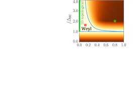
Figure S2: (a) Schematic presentation of the resonance off-set in the anisotropic regime $\alpha_{x}\neq\alpha_{y}$ showing the SOI momentum $k_{\textrm{so}}(\theta)$ (black solid line), the two Fermi surfaces $k^{F}_{1\pm}(\theta)$ (red solid and green dotted lines) of the Floquet band $\tau=1$ and the Fermi surface $k^{F}_{\bar{1}-}(\theta)$ (blue dashed line) of the Floquet band $\tau=\bar{1}$. The coupling between the two Floquet bands occurs in the neighborhood of the Fermi surfaces $k^{F}_{1-}(\theta)$ and $k^{F}_{\bar{1}+}(\theta)$ but, due to the SOI anisotropy, a mismatch $\delta k=k^{F}_{\bar{1}+}(\theta)-k^{F}_{1-}(\theta)$ (orange filled surface) emerges. (b) Phase diagram showing the gap to the first excited bulk state (in units of $E_{\textrm{so}}$) as a function of the ratios $r=m_{x}/m_{y}=(\alpha_{y}/\alpha_{x})^{1/q}$ and $t_{\textrm{Z}}^{\perp}/\Delta_{\textrm{sc}}$ for $q=1$. Different colors and line types of the phase boundaries correspond to different power laws with $q=1$ (blue solid), $q=2$ (purple dashed), $q=3$ (red dotted). (c)-(d) Probability density of the lowest energy state and the band structure $E(k_{x})$ (in the inset) in different regions of the phase diagram. The choice of parameters $t^{\perp}_{\textrm{F}}/\Delta_{\textrm{sc}}$ and $r$ is indicated by the red square and the green star in (b). Remaining parameters in all the simulations are $t_{\textrm{Z}}^{\parallel}=0$, $\Delta_{\textrm{sc}}/E_{\textrm{so}}=0.2$, $k_{\textrm{so}}a=0.2$, $k_{\textrm{so}}L_{x}=k_{\textrm{so}}L_{y}=80$, and $\mu=-E_{\textrm{so}}/2$.

S4.  Discretized model

In the discretized version of our model, the creation (annihilation) operators $\psi^{{\dagger}}_{\tau\sigma mn}$ ($\psi_{\tau\sigma mn}$) of an electron with spin component $\sigma$ along the $z$ axis, in a Floquet band $\tau$, are defined at discrete coordinate sites $n$ and $m$. For simplicity, we assume that the lattice constant $a$ is the same in $x$ and $y$ directions. The Hamiltonian describing the anisotropic 2DEG, or equivalently the array of coupled Rashba wires, corresponds to

$$H_{0}=\sum\limits_{mn}\sum\limits_{\tau}\Big{\{}\Big{[}- t_{x}\left(\psi^{{\dagger}}_{\tau\uparrow m(n+1)}\psi_{\tau\uparrow mn}+\psi^{{\dagger}}_{\tau\downarrow m(n+1)}\psi_{\tau\downarrow mn}\right)-t_{y}\left(\psi^{{\dagger}}_{\tau\uparrow(m+1)n}\psi_{\tau\uparrow mn}+\psi^{{\dagger}}_{\tau\downarrow(m+1)n}\psi_{\tau\downarrow mn}\right)$$

$$- \tilde{\alpha}_{x}\left(\psi^{{\dagger}}_{\tau\uparrow(m+1)n}\psi_{\tau\downarrow mn}-\psi^{{\dagger}}_{\tau\uparrow mn}\psi_{\tau\downarrow(m+1)n}\right)+\tilde{\alpha}_{y}i\left(\psi^{{\dagger}}_{\tau\uparrow(m+1)n}\psi_{\tau\downarrow mn}-\psi^{{\dagger}}_{\tau\uparrow mn}\psi_{\tau\downarrow(m+1)n}\right)+\textrm{H.c.}\Big{]}$$

$$+ \sum\limits_{\sigma}\left(2t_{x}+2t_{y}-\mu\right)\psi^{{\dagger}}_{\tau\sigma mn}\psi_{\tau\sigma mn}\Big{\}}\;.$$ (S20)

Here, $t_{x}=\hbar^{2}/(2m_{x}a^{2})$ and $t_{y}=\hbar^{2}/(2m_{y}a^{2})$. The spin-flip hopping amplitudes $\tilde{\alpha}_{x}$ and $\tilde{\alpha}_{y}$ are related to the corresponding SOI strengths of the continuum model via $\alpha_{y}/\tilde{\alpha}_{y}=\alpha_{x}/\tilde{\alpha}_{x}=2a$. The proximity induced $s$-wave superconducting term is expressed as

$$H_{\textrm{sc}}=-\frac{\Delta_{\textrm{sc}}}{2}\sum\limits_{mn}\sum\limits_{\tau}\left(\psi^{{\dagger}}_{\tau\uparrow mn}\psi^{{\dagger}}_{\tau\downarrow mn}-\psi^{{\dagger}}_{\tau\downarrow mn}\psi^{{\dagger}}_{\tau\uparrow mn}+\textrm{H.c.}\right)\;.$$ (S21)

The out-of-plane component of the Floquet-Zeeman coupling is

$$H_{\textrm{Z}}^{\perp}=t_{\textrm{Z}}^{\perp}\sum\limits_{mn}\left(\psi^{{\dagger}}_{1\uparrow mn}\psi_{\bar{1}\uparrow mn}-\psi^{{\dagger}}_{1\downarrow mn}\psi_{\bar{1}\downarrow mn}+\textrm{H.c.}\right)-\hbar\omega\sum\limits_{mn}\sum\limits_{\sigma}\psi^{{\dagger}}_{\bar{1}\sigma mn}\psi_{\bar{1}\sigma mn}\;,$$ (S22)

where the second term describes the constant energy shift of the second Floquet band with respect to the first one. It incorporates the $i\hbar\partial_{t}$-term which is present in the expression of the quasi-energy operator written in the basis of $T$-periodic states. We finally express the in-plane component of the Floquet-Zeeman term as

$$H_{\textrm{Z}}^{\parallel}=t_{\textrm{Z}}^{\parallel}\sum\limits_{mn}\sum\limits_{\tau\sigma\sigma^{\prime}}\psi^{{\dagger}}_{\tau\sigma mn}\left[\bm{u}_{\parallel}\cdot\bm{\sigma}\right]_{\sigma\sigma^{\prime}}\psi_{\bar{\tau}\sigma^{\prime}mn}\;.$$ (S23)

In the presence of translation symmetry, the total Hamiltonian $H=H_{0}+H_{\textrm{sc}}+H_{\textrm{Z}}^{\perp}+H_{\textrm{Z}}^{\parallel}$ can be diagonalized in momentum space as $H=\sum_{\bm{k}}\Psi^{{\dagger}}_{\bm{k}}\mathcal{H}_{\bm{k}}\Psi_{\bm{k}}/2$, leading to

$$\mathcal{H}_{\bm{k}}= \Big{(}2t_{x}\left[1-\cos(k_{x}a)\right]+2t_{y}\left[1-\cos(k_{y}a)\right]-\mu\Big{)}\eta_{z}-2\tilde{\alpha}_{x}\sin(k_{x}a)\eta_{z}\sigma_{y}+2\tilde{\alpha}_{y}\sin(k_{y}a)\sigma_{x}$$

$$+ \Delta_{\textrm{sc}}\eta_{y}\sigma_{y}+t_{\textrm{Z}}^{\perp}\eta_{z}\tau_{x}\sigma_{z}+t_{\textrm{Z}}^{\parallel}\left(u_{x}\tau_{y}\sigma_{x}+u_{y}\eta_{z}\tau_{y}\sigma_{y}\right)+\hbar\omega\eta_{z}\left(\frac{\tau_{z}-\tau_{0}}{2}\right)\;.$$ (S24)

The explicit representation of the Hamiltonian as $8\times 8$ matrix reads

$$\mathcal{H}_{\bm{k}}=\left(\begin{array}[]{cccccccc}\lambda_{\bm{k}}&\alpha_{k_{y}}+i\alpha_{k_{x}}&t_{\textrm{Z}}^{\perp}&t_{\textrm{Z}}^{\parallel}\left(-u_{y}-iu_{x}\right)&0&-\Delta_{\textrm{sc}}&0&0\\ \alpha_{k_{y}}-i\alpha_{k_{x}}&\lambda_{\bm{k}}&t_{\textrm{Z}}^{\parallel}\left(u_{y}-iu_{x}\right)&-t_{\textrm{Z}}^{\perp}&\Delta_{\textrm{sc}}&0&0&0\\ t_{\textrm{Z}}^{\perp}&t_{\textrm{Z}}^{\parallel}\left(u_{y}+iu_{x}\right)&\lambda_{\bm{k}}-\hbar\omega&\alpha_{k_{y}}+i\alpha_{k_{x}}&0&0&0&-\Delta_{\textrm{sc}}\\ t_{\textrm{Z}}^{\parallel}\left(-u_{y}+iu_{x}\right)&-t_{\textrm{Z}}^{\perp}&\alpha_{k_{y}}-i\alpha_{k_{x}}&\lambda_{\bm{k}}-\hbar\omega&0&0&\Delta_{\textrm{sc}}&0\\ 0&\Delta_{\textrm{sc}}&0&0&-\lambda_{\bm{k}}&\alpha_{k_{y}}-i\alpha_{k_{x}}&-t_{\textrm{Z}\perp}&t_{\textrm{Z}\parallel}\left(u_{y}-iu_{x}\right)\\ -\Delta_{\textrm{sc}}&0&0&0&\alpha_{k_{y}}+i\alpha_{k_{x}}&-\lambda_{\bm{k}}&t_{\textrm{Z}}^{\parallel}\left(-u_{y}-iu_{x}\right)&t_{\textrm{Z}}^{\perp}\\ 0&0&0&\Delta_{\textrm{sc}}&-t_{\textrm{Z}}^{\perp}&t_{\textrm{Z}}^{\parallel}\left(-u_{y}+iu_{x}\right)&-\lambda_{\bm{k}}+\hbar\omega&\alpha_{k_{y}}-i\alpha_{k_{x}}\\ 0&0&-\Delta_{\textrm{sc}}&0&t_{\textrm{Z}}^{\parallel}\left(u_{y}+iu_{x}\right)&t_{\textrm{Z}}^{\perp}&\alpha_{k_{y}}+i\alpha_{k_{x}}&-\lambda_{\bm{k}}+\hbar\omega\end{array}\right),$$ (S25)

where we introduced the notations $\lambda_{\bm{k}}=t_{x}\left[1-\cos(k_{x}a)\right]+t_{y}\left[1-\cos(k_{y}a)\right]-\mu/2$, ${\alpha_{k_{x}}=\tilde{\alpha}_{x}\sin(k_{x}a)}$, and ${\alpha_{k_{y}}=\tilde{\alpha}_{y}\sin(k_{y}a)}$.

S5.   Micromagnetic simulations

As shown in the main text, to reach the topological phase transition one needs to generate a magnetic field $\bm{B}(t)$ with a magnitude of the order of $0.1$ T oscillating in the GHz frequency range. Moreover, the oscillating component of $\bm{B}(t)$ should be greater than the static one. One possible solution to generate such a magnetic field consists in placing the 2DEG layer in proximity to a FM slab. In this section we provide details of this construction.

At equilibrium, the magnetization $\bm{M}$ of the FM is aligned with the easy axis of the FM. For simplicity, we assume that the easy axis lies in the $xy$ plane, parallel to the bottom (and top) surface of the FM slab. We consider a time-dependent protocol, where the system at an initial time is subjected to a static external magnetic field $\bm{H}_{0}$, which makes an angle with the magnetization $\bm{M}$ but also lies in the $xy$ plane. Moreover, an additional small time-dependent magnetic field $\bm{h}(t)$ with $|\bm{h}(t)|\ll|\bm{H}_{0}|$ is applied perpendicularly to $\bm{H}_{0}$ such that the total applied external magnetic field is $\bm{H}(t)=\bm{H}_{0}+\bm{h}(t)$. As a result, the magnetization $\bm{M}(t)$ will start to precess, described by the Landau-Lifshitz-Gilbert (LLG) equation [9, 10]

$$\frac{\textrm{d}\bm{M}(t)}{\textrm{d}t}=-\gamma\bm{M}(t)\times\bm{B}(t)-\alpha\frac{\gamma}{M_{\textrm{s}}}\bm{M}(t)\times\left[\bm{M}(t)\times\bm{B}(t)\right]\;.$$ (S26)

Here, $\gamma$ is the gyromagnetic ratio, $\alpha$ the dimensionless damping factor, and $M_{\textrm{s}}$ the saturation magnetization. The total magnetic field $\bm{B}(t)=\bm{H}(t)+\bm{D}(t)$ comprises the applied static field $\bm{H}_{0}$, the small time-dependent field $\bm{h}(t)$, and the demagnetizing field $\bm{D}(t)$ generated by the FM. We note that the demagnetizing field has in general a complicated structure that depends on the shape of the FM as well as the crystalline anisotropy. The LLG equation can be solved under simplified conditions, by neglecting the small field $\bm{h}(t)$ and assuming that the demagnetizing field is constant: $\bm{D}(t)=\bm{D}$. Such a solution describes a damped precession of the magnetization with the frequency determined by the Kittel formula [11, 12]

$$\omega=\gamma\sqrt{|\bm{H}_{0}||\bm{H}_{0}+\bm{D}|}\;.$$ (S27)

Finally, if the small field $\bm{h}(t)$ is resonant at the frequency $\omega$, the FM absorbs energy, establishing a steady-state with a fixed precession angle of the magnetization.

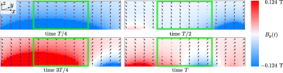
Figure S3: OOMMF simulations of the total effective field $\bm{B}(t)$ in a $50$ nm height pocket above the FM at four different moments of time in the interval $[0,T]$. Arrows represent the $x$ and $z$ components of $\bm{B}(t)$, while the intensity plot represents its $y$ component. In the region inside the green box the static component of $\bm{B}(t)$ is much smaller than the oscillating part, and the effective field makes a full rotation in the $yz$ plane, corresponding to the optimal arrangement for our Floquet setup. In the region outside the green box the left (right) boundary of the FM is too close and no sizable precession of $\bm{B}(t)$ can develop there. The amplitude of the magnetic field is shown on the scale $[0,0.124]$ T. Parameters of the simulation are $L_{x}\times L_{y}\times L_{z}=200\times 200\times 100$ nm and $|\bm{H}_{0}|=0.124$ T.

The protocol described above allows one to generate a substantial large oscillating magnetic field through the demagnetizing field of the FM. However, generically the static component of such a magnetic field will dominate over the dynamic one, which is not desired for our purpose. This problem can be removed by adjusting the geometry of the setup (the size of the FM) and the strength of the applied static field $\bm{H}_{0}$, so that the static component of the demagnetizing field $\bm{D}(t)$ cancels $\bm{H}_{0}$ exactly. In Fig. S3 we show the result of a calculation, based on the numerical solution of the LLG equation using the finite difference micromagnetic solver OOMMF [13]. We find that for a FM slab of the size $L_{x}\times L_{y}\times L_{z}=200\times 200\times 100$ nm there is a wide region of the space distanced from the left and right boundaries of the FM, where the total effective field $\bm{B}(t)$ oscillates at the frequency $\omega=2\pi/T=63$ GHz and makes a full $360^{\circ}$ rotation in the $yz$ plane (which is optimal for our purpose). The initial parameters of the simulation are chosen such that the static field $\bm{H}_{0}$ with $|\bm{H}_{0}|=0.124$ T is directed along the $x$ axis. At the initial time the magnetization $\bm{M}$ makes an angle of $11.3^{\circ}$ with the vector $\bm{H}_{0}$. The amplitude of the resulting oscillating field $\bm{B}(t)$ is of the order of $0.1$ T.

References

- [1] M. Z. Hasan and C. L. Kane, Rev. Mod. Phys. 82, 3045 (2010).
- [2] X.-L. Qi and S.-C. Zhang, Rev. Mod. Phys. 83, 1057 (2011).
- [3] M. Sato and Y. Ando, Rep. Prog. Phys. 80, 076501 (2017).
- [4] J. Wang and S.-C. Zhang, Nat. Mat. 16, 1062-1067 (2017).
- [5] X.-G. Wen, Rev. Mod. Phys. 89, 41004 (2017).
- [6] W. A. Benalcazar, B. A. Bernevig, and T. L. Hughes, Science 357, 6346 (2017).
- [7] W. A. Benalcazar, B. A. Bernevig, and T. L. Hughes, Phys. Rev. B 96, 245115 (2017).
- [8] Z. Song, Z. Fang, and C. Fang, Phys. Rev. Lett. 119, 246402 (2017).
- [9] Y. Peng, Y. Bao, and F. von Oppen, Phys. Rev. B 95, 235143 (2017).
- [10] S. Imhof, C. Berger, F. Bayer, J. Brehm, L. W. Molenkamp, T. Kiessling, F. Schindler, C. Hua Lee, M. Greiter, T. Neupert, and R. Thomale, Nat. Phys. 14, 925 (2018).
- [11] M. Geier, L. Trifunovic, M. Hoskam, and P. W. Brouwer, Phys. Rev. B 97, 205135 (2018).
- [12] F. Schindler, A. M. Cook, M. G. Vergniory, Z. Wang, S. S. P. Parkin, B. A. Bernevig, and T. Neupert, Science Adv. 4, 6 (2018).
- [13] C.-H. Hsu, P. Stano, J. Klinovaja, and D. Loss, Phys. Rev. Lett. 121, 196801 (2018).
- [14] T. Liu, J. J. He, and F. Nori, Phys. Rev. B 98, 245413 (2018).
- [15] Y. Volpez, D. Loss, and J. Klinovaja, Phys. Rev. Lett. 122, 126402 (2019).
- [16] M. Ezawa, Scientific Reports 9, 5286 (2019).
- [17] A. Agarwala, V. Juricic, B. Roy, arXiv:1902.00507.
- [18] K. Laubscher, D. Loss, and J. Klinovaja, arXiv:1905.00885.
- [19] D. Calugaru, V. Juricic, and B. Roy, Phys. Rev. B 99, 041301(R) (2019).
- [20] S. Franca, J. van den Brink, and I. C. Fulga, Phys. Rev. B 98, 201114(R) (2018).
- [21] R. W. Bomantara, L. Zhou, J. Pan, and J. Gong, Phys. Rev. B 99, 045441 (2019).
- [22] Y. Peng and G. Refael, arXiv:1811.11752 (2018).
- [23] B. Huang and W. V. Liu, arXiv:1811.00555 (2018).
- [24] M. Rodriguez-Vega, A. Kumar, and B. Seradjeh, arXiv:1811.04808 (2018).
- [25] R. Seshadri, A. Dutta, and D. Sen, arXiv:1901.10495 (2019).
- [26] T. Nag, V. Juricic, B. Roy, arXiv:1904.07247 (2019).
- [27] J. H. Shirley, Phys. Rev. 138, 979 (1965).
- [28] N. Goldman and J. Dalibard, Phys. Rev. X 4, 031027 (2014).
- [29] M. Bukov, L. D’Alessio, and A. Polkovnikov, Advances in Physics 64, 2, 139 (2015).
- [30] A. Eckardt and E. Anisimovas, New. J. Phys. 17, 093039 (2015).
- [31] T. Oka and H. Aoki, Phys. Rev. B 79, 081406(R) (2009).
- [32] J.-I. Inoue and A. Tanaka, Phys. Rev. Lett. 105, 017401 (2010).
- [33] T. Kitagawa, T. Oka, A. Brataas, L. Fu, and E. Demler, Phys. Rev. B 84, 235108 (2011).
- [34] N. H. Lindner, G. Refael, and V. Galitski, Nat. Phys. 7, 490 (2011).
- [35] N. H. Lindner, D. L. Bergman, G. Refael, and V. Galitski, Phys. Rev. B 87, 235131 (2013).
- [36] J. Cayssol, B. Dóra, F. Simon, and R. Moessner, Phys. Status Solidi RRL, 7, 101 (2013).
- [37] P. M. Perez-Piskunow, G. Usaj, C. A. Balseiro, and L. E. F. Foa Torres, Phys. Rev. B 89, 121401(R).
- [38] J. Klinovaja, P. Stano, and D. Loss, Phys. Rev. Lett. 116, 176401 (2016).
- [39] T. Kitagawa, M. A. Broome, A. Fedrizzi, M. S. Rudner, E. Berg, I. Kassal, A. Aspuru-Guzik, E. Demler, and A. G. White, Nat. Comm. 3, 882 (2012).
- [40] M. C. Rechtsman, J. M. Zeuner, Y. Plotnik, Y. Lumer, D. Podolsky, F. Dreisow, S. Nolte, M. Segev, and A. Szameit, Nature 496, 196 (2013).
- [41] M. Aidelsburger, M. Atala, M. Lohse, J. T. Barreiro, B. Paredes, and I. Bloch, Phys. Rev. Lett. 111, 185301 (2013).
- [42] G. Jotzu, M. Messer, R. Desbuquois, M. Lebrat, T. Uehlinger, D. Greif, and T. Esslinger, Nature 515, 237 (2014).
- [43] K. Le Hur, L. Henriet, A. Petrescu, K. Plekhanov, G. Roux, and M. Schiró, C. R. Physique 17, 808 (2016).
- [44] T. Kitagawa, E. Berg, M. Rudner, and E. Demler, Phys. Rev. B 82, 235114 (2010).
- [45] M. S. Rudner, N. H. Lindner, E. Berg, and M. Levin, Phys. Rev. X 3, 031005 (2013).
- [46] R. Roy and F. Harper, Phys. Rev. B 96, 155118 (2017).
- [47] L. J. Maczewsky, J. M. Zeuner, S. Nolte, and A. Szameit, Nat. Comm. 8, 13756 (2017).
- [48] S. Yao, Z. Yan, and Z. Wang, Phys. Rev. B 96, 195303 (2017).
- [49] G. M. Graf and C. Tauber, Annales Henri Poincaré, 19, 709 (2018).
- [50] A. G. Grushin, Á. Gómez-León, and T. Neupert, Phys. Rev. Lett. 112, 156801 (2014).
- [51] L. Jiang, T. Kitagawa, J. Alicea, A. R. Akhmerov, D. Pekker, G. Refael, J. I. Cirac, E. Demler, M. D. Lukin, and P. Zoller, Phys. Rev. Lett. 106, 220402 (2011).
- [52] A. A. Reynoso and D. Frustaglia, Phys. Rev. B 87, 115420 (2013).
- [53] M. Thakurathi, A. A. Patel, D. Sen, and A. Dutta, Phys. Rev. B 88, 155133 (2013).
- [54] D. E. Liu, A. Levchenko, and H. U. Baranger, Phys. Rev. Lett. 111, 047002 (2013).
- [55] A. Kundu and B. Seradjeh, Phys. Rev. Lett. 111, 136402 (2013).
- [56] M. Thakurathi, K. Sengupta, and D. Sen, Phys. Rev. B 89, 235434 (2014).
- [57] M. Thakurathi, D. Loss, and J. Klinovaja, Phys. Rev. B 95, 155407 (2017).
- [58] D. M. Kennes, N. Müller, M. Pletyukhov, C. Weber, C. Bruder, F. Hassler, J. Klinovaja, D. Loss, H. Schoeller, arXiv:1811.12062 (2018).
- [59] D. T. Liu, J. Shabani, and A. Mitra, Phys. Rev. B 99, 094303 (2019).
- [60] E. I. Rashba, Sov. Phys. Solid State 2, 1109 (1960).
- [61] C. Kloeffel, D. Loss, Annu. Rev. Condens. Matter Phys. 4, 51 (2013).
- [62] A. I. Buzdin, Rev. Mod. Phys. 77, 935 (2005).
- [63] B. Li, N. Roschewsky, B. A. Assaf, M. Eich, M. Epstein-Martin, D. Heiman, M. Münzenberg, and J. S. Moodera, Phys. Rev. Lett. 110, 097001 (2013).
- [64] F. Katmis, V. Lauter, F. S. Nogueira, B. A. Assaf, M. E. Jamer, P. Wei, B. Satpati, J. W. F., I. Eremin, D. Heiman, P. Jarillo-Herrero, and J. S. Moodera, Nature 533, 513 (2016).
- [65] A. Kandala, A. Richardella, D. W. Rench, D. M. Zhang, T. C. Flanagan, and N. Samarth, Appl. Phys. Lett. 103, 202409 (2013).
- [66] Z. Jiang, C.-Z. Chang, C. Tang, J.-G. Zheng, J. S. Moodera, and J. Shi, AIP Advances 6, 055809 (2016).
- [67] J. Nitta, T. Akazaki, H. Takayanagi, and T. Enoki, Phys. Rev. Lett. 78, 1335 (1997).
- [68] G. Engels, J. Lange, T. Schapers, and H. Luth, Phys. Rev. B 55, R1958 (1997).
- [69] J. Schliemann, J. C. Egues, and D. Loss, Phys. Rev. Lett. 90, 146801 (2003).
- [70] B. A. Bernevig, J. Orenstein, and S. C. Zhang, Phys. Rev. Lett. 97, 236601 (2006).
- [71] R. Winkler, Spin-Orbit Coupling Effects in Two-Dimensional Electron and Hole Systems (Springer, Berlin, 2003).
- [72] J. D. Koralek, C. P. Weber, J. Orenstein, B. A. Bernevig, S.-C. Zhang, S. Mack, and D. D. Awschalom, Nature 458, 610 (2009).
- [73] M. Duckheim, D. L. Maslov, and D. Loss, Phys. Rev. B 80, 235327 (2009).
- [74] T. Meng, J. Klinovaja, and D. Loss, Phys. Rev. B 89, 205133 (2014).
- [75] C. L. Kane, R. Mukhopadhyay, and T. C. Lubensky, Phys. Rev. Lett. 88, 036401 (2002).
- [76] D. Poilblanc, G. Montambaux, M. Héritier, and P. Lederer, Phys. Rev. Lett. 58, 270 (1987).
- [77] L. P. Gor’kov and A. G. Lebed, Phys. Rev. B 51, 3285 (1995).
- [78] J. Klinovaja and D. Loss, Phys. Rev. Lett. 111, 196401 (2013).
- [79] J. C. Y. Teo and C. L. Kane, Phys. Rev. B 89, 085101 (2014).
- [80] J. Klinovaja and D. Loss, Eur. Phys. J. B 87, 171 (2014)
- [81] T. Meng, P. Stano, J. Klinovaja, and D. Loss, Eur. Phys. J. B 87, 203 (2014).
- [82] T. Neupert, C. Chamon, C. Mudry, and R. Thomale, Phys. Rev. B 90, 205101 (2014).
- [83] E. Sagi and Y. Oreg, Phys. Rev. B 90, 201102(R) (2014).
- [84] J. Klinovaja, Y. Tserkovnyak, and D. Loss, Phys. Rev. B 91, 085426 (2015).
- [85] R. A. Santos, C.-W. Huang, Y. Gefen, and D. B. Gutman, Phys. Rev. B 91, 205141 (2015).
- [86] P.-H. Huang, J.-H. Chen, P. R. S. Gomes, T. Neupert, C. Chamon, and C. Mudry, Phys. Rev. B 93, 205123 (2016).
- [87] P. Le Jeune, D. Robart, X. Marie, T. Amand, M. Brosseau, J. Barrau, and V. Kalevcih, Semicond. Sci. Technol. 12, 380 (1997).
- [88] A. Malinowski and R. T. Harley, Phys. Rev. B 62, 2051 (2000).
- [89] M. A. Toloza Sandoval, A. Ferreira da Silva, E. A. de Andrada e Silva, and G. C. La Rocca, Phys. Rev. B 86, 195302 (2012).
- [90] See the Supplemental Material for (i) details of derivation the topological criterion; (ii) an analytical description of helical edge modes and Majorana corner states; (iii) a study of the role of anisotropy on the topological phase diagram; (iv) an explicit form of the discretized Hamiltonian used in numerical calculations; (v) micromagnetic simulations of the magnetization dynamics in the driven triple-layer setup.
- [91] The initial presence of the effective symmerty is not crucial for our setup, as this symmetry is broken by the in-plane field anyway, thus, our setup is stable against disorder and does not rely on the presence of particular spatial symmetries.
- [92] R. Jackiw and C. Rebbi, Phys. Rev. D 13, 3398 (1976).
- [93] R. Jackiw and J. Schrieffer, Nucl. Phys. B 190, 253 (1981).
- [94] W. Chang, S. M. Albrecht, T. S. Jespersen, F. Kuemmeth, P. Krogstrup, J. Nygard, and C. M. Marcus, Nat. Nan. 10, 232 (2015).
- [95] Z. Wan, A. Kazakov, M. J. Manfra, L. N. Pfeiffer, K. W. West, and L. P. Rokhinson, Nat. Comm. 6, 7426 (2015).
- [96] C. Reeg, D. Loss, and J. Klinovaja, Beilstein J. of Nanotechnol. 9, 1263 (2018).
- [97] C. Kittel, Phys. Rev. 73, 155 (1948).
- [98] C. Kittel, J. Phys. Radium 12, 3 (1951).
- [99] C. D. Stanciu and F. Hansteen, A. V. Kimel, A. Kirilyuk, A. Tsukamoto, A. Itoh, and T. Rasing, Phys. Rev. Lett. 99, 047601 (2007).
- [100] A. Kirilyuk, A. V. Kimel, and T. Rasing, Rev. Mod. Phys. 82, 2731 (2010).
- [101] S. Higashikawa, H. Fujita, M. Sato, arXiv:1810.01103 (2018).
- [102] R.-C. Peng, J.-M. Hu, K. Momeni, J.-J. Wang, L.-Q. Chen, and C.-W. Nan, Scientific Reports 6, 27561 (2016).
- [103] Q. Wang, J. Domann, G. Yu, A. Barra, K. L. Wang, and G. P. Carman, Phys. Rev. Applied 10, 034052 (2018).
- [104] I. M. Miron, K. Garello, G. Gaudin, P.-J. Zermatten, M. V. Costache, S. Auffret, S. Bandiera, B. Rodmacq, A. Schuhl, and P. Gambardella. Nature 476, 189 (2011).
- [105] L. Liu, C.-F. Pai, Y. Li, H. W. Tseng, D. C. Ralph, and R. A. Buhrman, Science 336, 6081 (2012).
- [106] P. Gambardella and I. M. Miron, Phil. Trans. R. Soc. A 369, 3175 (2011).
- [107] J. Sinova, S. O. Valenzuela, J. Wunderlich, C. H. Back, and T. Jungwirth, Rev. Mod. Phys. 87, 1213 (2015).
- [108] A. Manchon, I. M. Miron, T. Jungwirth, J. Sinova, J. Zelezný, A. Thiaville, K. Garello, and P. Gambardella, arXiv:1801.09636 (2018).
Supplemental Material: Floquet Second-Order Topological Superconductor

References

- [1] J. H. Shirley, Phys. Rev. 138, 979 (1965).
- [2] N. Goldman and J. Dalibard, Phys. Rev. X 4, 031027 (2014).
- [3] M. Bukov, L. D’Alessio, and A. Polkovnikov, Advances in Physics 64, 2, 139 (2015).
- [4] A. Eckardt and E. Anisimovas, New. J. Phys. 17, 093039 (2015).
- [5] J. Klinovaja and D. Loss, Phys. Rev. B 86, 085408 (2012).
- [6] J. Klinovaja and D. Loss, Eur. Phys. J. B 88, 62 (2015).
- [7] R. Jackiw and C. Rebbi, Phys. Rev. D 13, 3398 (1976).
- [8] R. Jackiw and J. Schrieffer, Nucl. Phys. B 190, 253 (1981).
- [9] L. D. Landau and E. M. Lifshitz, Phys. Z. Sowjetunion. 8, 153 (1935).
- [10] T. L. Gilbert, Phys. Rev. 100, 1235 (1955).
- [11] C. Kittel, Phys. Rev. 73, 155 (1948).
- [12] C. Kittel, J. Phys. Radium 12, 3 (1951).
- [13] M. J. Donahue and D. G. Porter, “OOMMF User’s Guide, Version 1.0”, NISTIR 6376 (1999).