Arbitrary high-order, conservative and positive preserving Patankar-type deferred correction schemes

Philipp Öffner  and Davide Torlo
Institute of Mathematics, University of Zurich, Switzerland
Corresponding author: P. Öffner, philipp.oeffner@math.uzh.chCorresponding author: D. Torlo, davide.torlo@math.uzh.ch
(August 6th, 2019)
Abstract

Production-destruction systems (PDS) of ordinary differential equations (ODEs) are used to describe physical and biological reactions in nature. The considered quantities are subject to natural laws. Therefore, they preserve positivity and conservation of mass at the analytical level.

In order to maintain these properties at the discrete level, the so-called modified Patankar-Runge-Kutta (MPRK) schemes are often used in this context. However, up to our knowledge, the family of MPRK has been only developed up to third order of accuracy. In this work, we propose a method to solve PDS problems, but using the Deferred Correction (DeC) process as a time integration method. Applying the modified Patankar approach to the DeC scheme results in provable conservative and positivity preserving methods. Furthermore, we demonstrate that these modified Patankar DeC schemes can be constructed up to arbitrarily high order. Finally, we validate our theoretical analysis through numerical simulations.

1 Introduction

The modelling of geobiochemical processes or ecosystems leads often to systems of ordinary differential equations (ODEs) which can be formulated in the so-called production-destruction systems (PDS) as described in [5, 10] for example. To guarantee the physical and chemical laws, the quantities have to fulfil several conditions like positivity and conservation.

The applied numerical method should not violate these conditions and big efforts have been devoted to designing conservative and positivity preserving schemes, since classical approaches like Runge Kutta (RK) schemes do not guarantee these properties.

In [4] the authors suggest modified Patankar-type methods of first and second order which verify the desired properties, i.e., conservation and positivity. Recently, further extensions were done to construct modified Patankar-Runge-Kutta (MPRK) schemes of second and third order [14, 16, 15, 12, 11]. As the name suggests, all these schemes use, as a basic procedure, the Runge-Kutta method, which has been modified by weighting the production and destruction terms as suggested in [20]. Thanks to these weighting coefficients, the schemes are forced to maintain positivity of the variables and to conserve some quantities of interest. However, the described and constructed schemes are, up to our knowledge, at most third order accurate.

In this paper, we present a way to construct arbitrary high-order, positivity preserving, numerically robust and conservative schemes for PDS. Differently from previous schemes, we do not start building our schemes on RK methods. We consider the Deferred Correction (DeC) procedure, a high order time integration technique, and we modify it, in order to obtain a positivity preserving, conservative and arbitrary high-order scheme. Moreover, we provide a proof of the desired properties.

The paper is organised as follows.
In section 2 we introduce the production-destruction systems and we give a short introduction about the so-called Patankar trick and how it was applied in [5] to construct a modified Patankar-type scheme starting from the explicit Euler method. Afterwards, in section 3, we introduce the Deferred Correction (DeC) method and we discuss conservation and positivity for this classical formulation. In section 4, we build the main core of this work, explaining our modification of DeC through the Patankar trick (mPDeC) and we prove that the obtained mPDeC schemes are positive preserving, conservative and arbitrary high-order accurate. In section 5, we validate our theoretical investigations, considering three different benchmark problems, which are also discussed in different literature references, as [4, 14]. Finally, we give a summary and an outlook for possible extensions.

2 Production–Destruction Systems

In this paper we consider production-destruction systems (PDS) of the form

{dtci=Pi(𝐜)Di(𝐜),i=1,,I,𝐜(t=0)=𝐜0,casesformulae-sequencesubscript𝑑𝑡subscript𝑐𝑖subscript𝑃𝑖𝐜subscript𝐷𝑖𝐜𝑖1𝐼otherwise𝐜𝑡0subscript𝐜0otherwise\begin{cases}d_{t}c_{i}=P_{i}(\mathbf{c})-D_{i}(\mathbf{c}),\quad i=1,\dots,I,\\ \mathbf{c}(t=0)=\mathbf{c}_{0},\end{cases} (1)

where 𝐜=(c1,,cI)TI𝐜superscriptsubscript𝑐1subscript𝑐𝐼𝑇superscript𝐼\mathbf{c}=(c_{1},\dots,c_{I})^{T}\in\mathbb{R}^{I} represents the vectors of I𝐼I constituents, t𝑡t denotes the time and 𝐜0subscript𝐜0\mathbf{c}_{0} the initial condition. Moreover, Pi(𝐜)subscript𝑃𝑖𝐜P_{i}(\mathbf{c}) and Di(𝐜)subscript𝐷𝑖𝐜D_{i}(\mathbf{c}) represent the production and destruction rates of the i𝑖i-th constituent and both terms are assumed to be non-negative, i.e, Pi,Di0subscript𝑃𝑖subscript𝐷𝑖0P_{i},\;D_{i}\geq 0 for i=1,,I𝑖1𝐼i=1,\dots,I. These systems rise naturally to describe geochemical processes as it is described in [4, 5] and we recapitulate their notations and definitions in this section.
The production and destruction terms can also be written in a matrix form as follows

Pi(𝐜)=j=1Ipi,j(𝐜),Di(𝐜)=j=1Idi,j(𝐜),formulae-sequencesubscript𝑃𝑖𝐜superscriptsubscript𝑗1𝐼subscript𝑝𝑖𝑗𝐜subscript𝐷𝑖𝐜superscriptsubscript𝑗1𝐼subscript𝑑𝑖𝑗𝐜P_{i}(\mathbf{c})=\sum_{j=1}^{I}p_{i,j}(\mathbf{c}),\quad D_{i}(\mathbf{c})=\sum_{j=1}^{I}d_{i,j}(\mathbf{c}), (2)

where each term pi,j0subscript𝑝𝑖𝑗0p_{i,j}\geq 0 and di,j0subscript𝑑𝑖𝑗0d_{i,j}\geq 0 are Lipschitz continuous functions and may depend linearly or non–linearly on 𝐜𝐜\mathbf{c}. Furthermore, the term di,jsubscript𝑑𝑖𝑗d_{i,j} describes the rate of change from the i𝑖i-th to the j𝑗j-th constituent while pi,jsubscript𝑝𝑖𝑗p_{i,j} is the rate at which the j𝑗j-th constituent is transformed into the i𝑖i-th.
We are interested in (fully) conservative and positive production–destruction systems. To clarify these expressions we repeat the definitions from [14].

Definition 2.1.

The PDS (1) is called positive if positive initial values ci(0)>0subscript𝑐𝑖00c_{i}(0)>0 for i=1,,I𝑖1𝐼i=1,\dots,I imply positive solutions, ci(t)>0subscript𝑐𝑖𝑡0c_{i}(t)>0 for i=1,,I𝑖1𝐼i=1,\cdots,I for all times t>0𝑡0t>0.
The PDS (1) is called conservative if at any time t0𝑡0t\geq 0, we have that

i=1Ici(t)=i=1Ici(0)superscriptsubscript𝑖1𝐼subscript𝑐𝑖𝑡superscriptsubscript𝑖1𝐼subscript𝑐𝑖0\sum_{i=1}^{I}c_{i}(t)=\sum_{i=1}^{I}c_{i}(0) (3)

is fulfilled. In the analytic form (1), the conservation property (3) is equivalent to the following relation for the matrix representation (2)

pi,j(𝐜)=dj,i(𝐜),i,j=1,,I.formulae-sequencesubscript𝑝𝑖𝑗𝐜subscript𝑑𝑗𝑖𝐜for-all𝑖𝑗1𝐼p_{i,j}(\mathbf{c})=d_{j,i}(\mathbf{c}),\quad\forall i,j=1,\dots,I. (4)

Moreover, the system is called fully conservative if additionally pi,i(𝐜)=di,i(𝐜)=0subscript𝑝𝑖𝑖𝐜subscript𝑑𝑖𝑖𝐜0p_{i,i}(\mathbf{c})=d_{i,i}(\mathbf{c})=0 holds for all 𝐜0𝐜0\mathbf{c}\geq 0 and i=1,,I𝑖1𝐼i=1,\dots,I.

As it is described in [14] every conservation PDS can be written in a fully conservative formulation. We can rewrite the two terms of (4) into one matrix of exchanging quantities e(𝐜)𝑒𝐜e(\mathbf{c}) defined as

ei,j(𝐜):=pi,j(𝐜)di,j(𝐜).assignsubscript𝑒𝑖𝑗𝐜subscript𝑝𝑖𝑗𝐜subscript𝑑𝑖𝑗𝐜e_{i,j}(\mathbf{c}):=p_{i,j}(\mathbf{c})-d_{i,j}(\mathbf{c}). (5)

Clearly, from property (4), we have that ei,i=0subscript𝑒𝑖𝑖0e_{i,i}=0. With this notation, let us define the total exchange rate for the i𝑖i-th constituent as

Ei(𝐜):=Pi(𝐜)Di(𝐜).assignsubscript𝐸𝑖𝐜subscript𝑃𝑖𝐜subscript𝐷𝑖𝐜E_{i}(\mathbf{c}):=P_{i}(\mathbf{c})-D_{i}(\mathbf{c}). (6)

A numerical method suited to solve a conservative and positive PDS (1) should mimic, at the discrete level, the continuous setting properties. For a one-step methods, we can introduce the discrete analogues of definitions (2.1).

Definition 2.2.

Let 𝐜nsuperscript𝐜𝑛\mathbf{c}^{n} denote the approximation of 𝐜(tn)𝐜superscript𝑡𝑛\mathbf{c}(t^{n}) at the time level tnsuperscript𝑡𝑛t^{n}. A one-step method

𝐜n+1=𝐜n+ΔtΦ(tn,𝐜n,𝐜n+1,Δt),superscript𝐜𝑛1superscript𝐜𝑛Δ𝑡Φsuperscript𝑡𝑛superscript𝐜𝑛superscript𝐜𝑛1Δ𝑡\mathbf{c}^{n+1}=\mathbf{c}^{n}+\Delta t\Phi(t^{n},\mathbf{c}^{n},\mathbf{c}^{n+1},\Delta t), (7)

with process function ΦΦ\Phi, is called

  • unconditionally conservative if for all n𝑛n\in\mathbb{N} and Δt>0Δ𝑡0\Delta t>0

    i=1Icin+1=i=1Icinsuperscriptsubscript𝑖1𝐼subscriptsuperscript𝑐𝑛1𝑖superscriptsubscript𝑖1𝐼superscriptsubscript𝑐𝑖𝑛\sum_{i=1}^{I}c^{n+1}_{i}=\sum_{i=1}^{I}c_{i}^{n} (8)

    holds;

  • unconditionally positive if for all Δt>0Δ𝑡0\Delta t>0 and 𝐜n>0superscript𝐜𝑛0\mathbf{c}^{n}>0, we have that 𝐜n+1>0superscript𝐜𝑛10\mathbf{c}^{n+1}>0.

Example 2.3.

Let us consider as an example the explicit Euler method. The method is defined by

𝐜n+1=𝐜n+ΔtEi(𝐜n).superscript𝐜𝑛1superscript𝐜𝑛Δ𝑡subscript𝐸𝑖superscript𝐜𝑛\mathbf{c}^{n+1}=\mathbf{c}^{n}+\Delta tE_{i}(\mathbf{c}^{n}). (9)

It is conservative since

i=1I(cin+1cin)=i=1I(cin+Δti=1I(pi,j(𝐜n)di,j(𝐜n))cin)=Δti=1I(pi,j(𝐜n)di,j(𝐜n))=0superscriptsubscript𝑖1𝐼superscriptsubscript𝑐𝑖𝑛1superscriptsubscript𝑐𝑖𝑛superscriptsubscript𝑖1𝐼superscriptsubscript𝑐𝑖𝑛Δ𝑡superscriptsubscript𝑖1𝐼subscript𝑝𝑖𝑗superscript𝐜𝑛subscript𝑑𝑖𝑗superscript𝐜𝑛superscriptsubscript𝑐𝑖𝑛Δ𝑡superscriptsubscript𝑖1𝐼subscript𝑝𝑖𝑗superscript𝐜𝑛subscript𝑑𝑖𝑗superscript𝐜𝑛0\sum_{i=1}^{I}\left(c_{i}^{n+1}-c_{i}^{n}\right)=\sum_{i=1}^{I}\left(c_{i}^{n}+\Delta t\sum_{i=1}^{I}\left(p_{i,j}(\mathbf{c}^{n})-d_{i,j}(\mathbf{c}^{n})\right)-c_{i}^{n}\right)=\Delta t\sum_{i=1}^{I}\left(p_{i,j}(\mathbf{c}^{n})-d_{i,j}(\mathbf{c}^{n})\right)=0 (10)

holds. Conversely, the explicit Euler method is not unconditionally positive. Consider a conservative and positive PDS (1) where we assume that the right hand side is not identical zero. Then, there exists a 𝐜n0superscript𝐜𝑛0\mathbf{c}^{n}\geq 0 such that 𝐏(𝐜𝐧)𝐃(𝐜𝐧)𝟎𝐏superscript𝐜𝐧𝐃superscript𝐜𝐧0\bf{P}(\mathbf{c}^{n})-\bf{D}(\mathbf{c}^{n})\neq 0. Since the PDS is conservative, we can at least find one constituent i{1,,I}𝑖1𝐼i\in\{1,\dots,I\}, where Di(𝐜n)>Pi(𝐜n)0subscript𝐷𝑖superscript𝐜𝑛subscript𝑃𝑖superscript𝐜𝑛0D_{i}(\mathbf{c}^{n})>P_{i}(\mathbf{c}^{n})\geq 0. Choosing

Δt>cinDi(𝐜n)Pi(𝐜n)>0,Δ𝑡superscriptsubscript𝑐𝑖𝑛subscript𝐷𝑖superscript𝐜𝑛subscript𝑃𝑖superscript𝐜𝑛0\Delta t>\frac{c_{i}^{n}}{D_{i}(\mathbf{c}^{n})-P_{i}(\mathbf{c}^{n})}>0, (11)

we obtain

cin+1=cin+Δt(Pi(𝐜n)Di(𝐜n))<cin+𝐜inDi(𝐜n)Pi(𝐜n)(Pi(𝐜n)Di(𝐜n))=cincin=0.superscriptsubscript𝑐𝑖𝑛1superscriptsubscript𝑐𝑖𝑛Δ𝑡subscript𝑃𝑖superscript𝐜𝑛subscript𝐷𝑖superscript𝐜𝑛superscriptsubscript𝑐𝑖𝑛superscriptsubscript𝐜𝑖𝑛subscript𝐷𝑖superscript𝐜𝑛subscript𝑃𝑖superscript𝐜𝑛subscript𝑃𝑖superscript𝐜𝑛subscript𝐷𝑖superscript𝐜𝑛superscriptsubscript𝑐𝑖𝑛superscriptsubscript𝑐𝑖𝑛0c_{i}^{n+1}=c_{i}^{n}+\Delta t\left(P_{i}(\mathbf{c}^{n})-D_{i}(\mathbf{c}^{n})\right)<c_{i}^{n}+\frac{\mathbf{c}_{i}^{n}}{D_{i}(\mathbf{c}^{n})-P_{i}(\mathbf{c}^{n})}\left(P_{i}(\mathbf{c}^{n})-D_{i}(\mathbf{c}^{n})\right)=c_{i}^{n}-c_{i}^{n}=0. (12)

This demonstrates the violation of the positivity for the explicit Euler method for unbounded timesteps ΔtΔ𝑡\Delta t.

To build an unconditionally positive numerical scheme, Patankar had the idea in [20] of weighting the destruction term in the original explicit Euler methods with the following coefficient

cin+1=cin+Δt(j=1Ipi,j(𝐜n)j=1Idi,j(𝐜n)cin+1cin),i=1,,I.formulae-sequencesuperscriptsubscript𝑐𝑖𝑛1superscriptsubscript𝑐𝑖𝑛Δ𝑡superscriptsubscript𝑗1𝐼subscript𝑝𝑖𝑗superscript𝐜𝑛superscriptsubscript𝑗1𝐼subscript𝑑𝑖𝑗superscript𝐜𝑛subscriptsuperscript𝑐𝑛1𝑖superscriptsubscript𝑐𝑖𝑛𝑖1𝐼c_{i}^{n+1}=c_{i}^{n}+\Delta t\left(\sum_{j=1}^{I}p_{i,j}(\mathbf{c}^{n})-\sum_{j=1}^{I}d_{i,j}(\mathbf{c}^{n})\frac{c^{n+1}_{i}}{c_{i}^{n}}\right),\quad i=1,\dots,I. (13)

Hence, the scheme (13) is unconditionally positive, but the conservation relation is violated. In [4] a modification of the Patankar scheme (13) was presented, resulting in an unconditionally positive and conservative method. It is defined as follows.

cin+1:=cin+Δt(j=1Ipi,j(𝐜n)cjn+1cjnj=1Idi,j(𝐜n)cin+1cin),i=1,,I.formulae-sequenceassignsuperscriptsubscript𝑐𝑖𝑛1superscriptsubscript𝑐𝑖𝑛Δ𝑡superscriptsubscript𝑗1𝐼subscript𝑝𝑖𝑗superscript𝐜𝑛subscriptsuperscript𝑐𝑛1𝑗superscriptsubscript𝑐𝑗𝑛superscriptsubscript𝑗1𝐼subscript𝑑𝑖𝑗superscript𝐜𝑛subscriptsuperscript𝑐𝑛1𝑖superscriptsubscript𝑐𝑖𝑛𝑖1𝐼c_{i}^{n+1}:=c_{i}^{n}+\Delta t\left(\sum_{j=1}^{I}p_{i,j}(\mathbf{c}^{n})\frac{c^{n+1}_{j}}{c_{j}^{n}}-\sum_{j=1}^{I}d_{i,j}(\mathbf{c}^{n})\frac{c^{n+1}_{i}}{c_{i}^{n}}\right),\quad i=1,\dots,I. (14)

The scheme is implicit and can be solved inverting the mass matrix MM\mathrm{M} in the system M𝐜n+1=𝐜nMsuperscript𝐜𝑛1superscript𝐜𝑛\mathrm{M}\mathbf{c}^{n+1}=\mathbf{c}^{n} where MM\mathrm{M} is

{mi,i(𝐜n)=1+Δtk=1Idi,k(𝐜n)cin,i=1,,I,mi,j(𝐜n)=Δtpi,j(𝐜n)cjn,i,j=1,,I,ij.casesformulae-sequencesubscript𝑚𝑖𝑖superscript𝐜𝑛1Δ𝑡superscriptsubscript𝑘1𝐼subscript𝑑𝑖𝑘superscript𝐜𝑛superscriptsubscript𝑐𝑖𝑛𝑖1𝐼otherwiseformulae-sequencesubscript𝑚𝑖𝑗superscript𝐜𝑛Δ𝑡subscript𝑝𝑖𝑗superscript𝐜𝑛superscriptsubscript𝑐𝑗𝑛𝑖formulae-sequence𝑗1𝐼𝑖𝑗otherwise\begin{cases}m_{i,i}(\mathbf{c}^{n})=1+\Delta t\sum_{k=1}^{I}\frac{d_{i,k}(\mathbf{c}^{n})}{c_{i}^{n}},\quad i=1,\dots,I,\\ m_{i,j}(\mathbf{c}^{n})=-\Delta t\frac{p_{i,j}(\mathbf{c}^{n})}{c_{j}^{n}},\quad i,j=1,\dots,I,\,i\neq j.\end{cases} (15)

The construction of the mass matrix MM\mathrm{M} must follow substantial prescriptions in order to preserve the positivity of the scheme, as suggested in [15].

Remark 2.4.

Extensions of the modified Patankar scheme (14) to Runge-Kutta schemes were proposed in [14, 15] and further developed in [11, 12]. Special focus lies in the weighting of the production and destruction terms as it is investigated for example in [16] and references therein. Families of second and third order modified Patankar-Runge-Kutta (MPRK) schemes can be found in the mentioned literature. We do not provide the definition of MPRK because the modified Patankar scheme (14) already gives us the basic idea for the new methods we want to propose. We will prove that these methods are positivity preserving, conservative and arbitrary high-order.

3 Deferred Correction Methods

There are various approaches to solve numerically an ODE. A first approach is given by finite differences, where the derivative in time is replaced by differences of states in different timesteps. Backward and forward Euler are examples of this kind of strategy. Another approach would be to reformulate the ODE by integrating it in time. With different quadrature formulas and approximation techniques one can obtain various Runge-Kutta methods (explicit and implicit ones), see [9, 24] for details. However, we follow a different approach in this paper.
We start our investigation with the Deferred Correction (DeC) method introduced in [7]. In its original formulation, it is an explicit, arbitrary high order method for ODEs. Further extensions of DeC can be found in the literature, including semi-implicit approaches as in [19]. However, in this work we will not consider the semi-implicit framework. Instead, we will focus on the explicit DeC approach used by Abgrall in [1]. In our opinion, his notation describes DeC in a more compact way than in previous works [7, 6, 17].111We like to mention that Abgrall focused on DeC as a time integration scheme in the context of finite element methods. Applying a classical RK method, a dense mass matrix has to be inverted and Abgrall wanted to avoid this. By using a DeC scheme, instead, he showed that a mass matrix free approach is possible [1]. Nevertheless, the main idea is always the same and it is based on the Picard-Lindelöf theorem in the continuous setting. The theorem states the existence and uniqueness of solutions for ODEs. The classical proof makes use of the so-called Picard iterations to minimize the error and to prove convergence. The foundation of DeC relies on mimicking the Picard iterations at the discrete level. The approximation error decreases with several iteration steps. For the description of DeC, Abgrall introduces two operators: 1superscript1\mathcal{L}^{1} and 2superscript2\mathcal{L}^{2}.
Here, the 1superscript1\mathcal{L}^{1} operator represents a low-order easy-to-solve numerical scheme, e.g. the explicit Euler method, and 2superscript2\mathcal{L}^{2} is a high-order operator that can present difficulties in its practical solution, e.g. an implicit RK scheme. The DeC method can be written as a combination of these two operators.
Given a timeinterval [tn,tn+1]superscript𝑡𝑛superscript𝑡𝑛1[t^{n},t^{n+1}] we subdivide it into M𝑀M subintervals {[tn,m1,tn,m]}m=1Msuperscriptsubscriptsuperscript𝑡𝑛𝑚1superscript𝑡𝑛𝑚𝑚1𝑀\{[t^{n,m-1},t^{n,m}]\}_{m=1}^{M}, where tn,0=tnsuperscript𝑡𝑛0superscript𝑡𝑛t^{n,0}=t^{n} and tn,M=tn+1superscript𝑡𝑛𝑀superscript𝑡𝑛1t^{n,M}=t^{n+1} and we mimic for every subinterval [t0,tm]superscript𝑡0superscript𝑡𝑚[t^{0},t^{m}] the Picard–Lindelöf theorem for both operators 1superscript1\mathcal{L}^{1} and 2superscript2\mathcal{L}^{2}. We drop the dependency on the timestep n𝑛n for subtimesteps tn,msuperscript𝑡𝑛𝑚t^{n,m} and substates 𝐜m,nsuperscript𝐜𝑚𝑛\mathbf{c}^{m,n} as denoted in Figure 1.

tn=tn,0=t0superscript𝑡𝑛superscript𝑡𝑛0superscript𝑡0t^{n}=t^{n,0}=t^{0}\,\,\quad𝐜0superscript𝐜0\mathbf{c}^{0}tn,1=t1superscript𝑡𝑛1superscript𝑡1t^{n,1}=t^{1}𝐜1superscript𝐜1\mathbf{c}^{1}tn,m=tmsuperscript𝑡𝑛𝑚superscript𝑡𝑚t^{n,m}=t^{m}𝐜msuperscript𝐜𝑚\mathbf{c}^{m}tn,M=tM=tn+1superscript𝑡𝑛𝑀superscript𝑡𝑀superscript𝑡𝑛1\qquad t^{n,M}=t^{M}=t^{n+1}𝐜Msuperscript𝐜𝑀\mathbf{c}^{M}
Figure 1: Figure: divided time interval

Then, the 2superscript2\mathcal{L}^{2} operator is given by

2(𝐜0,,𝐜M):={𝐜M𝐜0t0tMM(E(𝐜0),,E(𝐜M))𝐜1𝐜0t0t1M(E(𝐜0),,E(𝐜M)).assignsuperscript2superscript𝐜0superscript𝐜𝑀casessuperscript𝐜𝑀superscript𝐜0superscriptsubscriptsuperscript𝑡0superscript𝑡𝑀subscript𝑀𝐸superscript𝐜0𝐸superscript𝐜𝑀otherwiseotherwisesuperscript𝐜1superscript𝐜0superscriptsubscriptsuperscript𝑡0superscript𝑡1subscript𝑀𝐸superscript𝐜0𝐸superscript𝐜𝑀otherwise\mathcal{L}^{2}(\mathbf{c}^{0},\dots,\mathbf{c}^{M}):=\begin{cases}\mathbf{c}^{M}-\mathbf{c}^{0}-\int_{t^{0}}^{t^{M}}\mathcal{I}_{M}(E(\mathbf{c}^{0}),\dots,E(\mathbf{c}^{M}))\\ \vdots\\ \mathbf{c}^{1}-\mathbf{c}^{0}-\int_{t^{0}}^{t^{1}}\mathcal{I}_{M}(E(\mathbf{c}^{0}),\dots,E(\mathbf{c}^{M}))\end{cases}. (16)

Here, the term Msubscript𝑀\mathcal{I}_{M} denotes an interpolation polynomial of order M𝑀M evaluated at the points {tn,r}r=0Msuperscriptsubscriptsuperscript𝑡𝑛𝑟𝑟0𝑀\{t^{n,r}\}_{r=0}^{M}. In particular, we use Lagrange polynomials {φr}r=0Msuperscriptsubscriptsubscript𝜑𝑟𝑟0𝑀\{\varphi_{r}\}_{r=0}^{M}, where φr(tn,m)=δr,msubscript𝜑𝑟superscript𝑡𝑛𝑚subscript𝛿𝑟𝑚\varphi_{r}(t^{n,m})=\delta_{r,m} and r=0Mφr(s)1superscriptsubscript𝑟0𝑀subscript𝜑𝑟𝑠1\sum_{r=0}^{M}\varphi_{r}(s)\equiv 1 for any s[0,1]𝑠01s\in[0,1]. Using these properties, we can actually compute the integral of the interpolants, thanks to a quadrature rule in the same points {tm}m=0Msuperscriptsubscriptsuperscript𝑡𝑚𝑚0𝑀\{t^{m}\}_{m=0}^{M} with weights θrm:=tntn,mφr(s)𝑑sassignsuperscriptsubscript𝜃𝑟𝑚superscriptsubscriptsuperscript𝑡𝑛superscript𝑡𝑛𝑚subscript𝜑𝑟𝑠differential-d𝑠\theta_{r}^{m}:=\int_{t^{n}}^{t^{n,m}}\varphi_{r}(s)ds. We can rewrite

2(𝐜0,,𝐜M)={𝐜M𝐜0r=0MθrME(𝐜r)𝐜1𝐜0r=0Mθr1E(𝐜r).superscript2superscript𝐜0superscript𝐜𝑀casessuperscript𝐜𝑀superscript𝐜0superscriptsubscript𝑟0𝑀superscriptsubscript𝜃𝑟𝑀𝐸superscript𝐜𝑟otherwiseotherwisesuperscript𝐜1superscript𝐜0superscriptsubscript𝑟0𝑀superscriptsubscript𝜃𝑟1𝐸superscript𝐜𝑟otherwise\mathcal{L}^{2}(\mathbf{c}^{0},\dots,\mathbf{c}^{M})=\begin{cases}\mathbf{c}^{M}-\mathbf{c}^{0}-\sum_{r=0}^{M}\theta_{r}^{M}E(\mathbf{c}^{r})\\ \vdots\\ \mathbf{c}^{1}-\mathbf{c}^{0}-\sum_{r=0}^{M}\theta_{r}^{1}E(\mathbf{c}^{r})\end{cases}. (17)

The 2superscript2\mathcal{L}^{2} operator represents an (M+1)𝑀1(M+1) order numerical scheme if set equal to zero, i.e., 2(𝐜0,,𝐜M)=0superscript2superscript𝐜0superscript𝐜𝑀0\mathcal{L}^{2}(\mathbf{c}^{0},\dots,\mathbf{c}^{M})=0. Unfortunately, the resulting scheme is implicit and, further, the terms E𝐸E may be non-linear. Because of this, the only 2superscript2\mathcal{L}^{2} formulation is not explicit and more efforts have to be made to solve it.

For this purpose, we introduce a simplification of the 2superscript2\mathcal{L}^{2} operator. Instead of using a quadrature formula at the points {tm}m=0Msuperscriptsubscriptsuperscript𝑡𝑚𝑚0𝑀\{t^{m}\}_{m=0}^{M} we evaluate the integral in equation (16) applying the left Riemann sum. The resulting operator 1superscript1\mathcal{L}^{1} is given by the forward Euler discretization for each state 𝐜msuperscript𝐜𝑚\mathbf{c}^{m} in the timeinterval, i.e.,

1(𝐜0,,𝐜M):={𝐜M𝐜0βMΔtE(𝐜0)𝐜1𝐜0β1ΔtE(𝐜0).assignsuperscript1superscript𝐜0superscript𝐜𝑀casessuperscript𝐜𝑀superscript𝐜0superscript𝛽𝑀Δ𝑡𝐸superscript𝐜0otherwiseotherwisesuperscript𝐜1superscript𝐜0superscript𝛽1Δ𝑡𝐸superscript𝐜0otherwise\mathcal{L}^{1}(\mathbf{c}^{0},\dots,\mathbf{c}^{M}):=\begin{cases}\mathbf{c}^{M}-\mathbf{c}^{0}-\beta^{M}\Delta tE(\mathbf{c}^{0})\\ \vdots\\ \mathbf{c}^{1}-\mathbf{c}^{0}-\beta^{1}\Delta tE(\mathbf{c}^{0})\end{cases}. (18)

with coefficients βm:=tmt0tMt0assignsuperscript𝛽𝑚superscript𝑡𝑚superscript𝑡0superscript𝑡𝑀superscript𝑡0\beta^{m}:=\frac{t^{m}-t^{0}}{t^{M}-t^{0}}.
To simplify the notation and to describe DeC, we introduce the vector of states for the variable 𝐜𝐜\mathbf{c} at all subtimesteps222We provide a table with all definitions and notations in the appendix A.

𝐜¯:=(𝐜0,,𝐜M)M×I, such thatformulae-sequenceassign¯𝐜superscript𝐜0superscript𝐜𝑀superscript𝑀𝐼 such that\displaystyle\underline{\mathbf{c}}:=(\mathbf{c}^{0},\dots,\mathbf{c}^{M})\in\mathbb{R}^{M\times I},\text{ such that } (19)
1(𝐜¯):=1(𝐜0,,𝐜M) and 2(𝐜¯):=2(𝐜0,,𝐜M).assignsuperscript1¯𝐜superscript1superscript𝐜0superscript𝐜𝑀 and superscript2¯𝐜assignsuperscript2superscript𝐜0superscript𝐜𝑀\displaystyle\mathcal{L}^{1}(\underline{\mathbf{c}}):=\mathcal{L}^{1}(\mathbf{c}^{0},\dots,\mathbf{c}^{M})\text{ and }\mathcal{L}^{2}(\underline{\mathbf{c}}):=\mathcal{L}^{2}(\mathbf{c}^{0},\dots,\mathbf{c}^{M}). (20)

Now, the DeC algorithm uses a combination of the 1superscript1\mathcal{L}^{1} and 2superscript2\mathcal{L}^{2} operators to provide an iterative procedure. The aim is to recursively approximate 𝐜¯superscript¯𝐜\underline{\mathbf{c}}^{*}, the numerical solution of the 2=0superscript20\mathcal{L}^{2}=0 scheme, similarly to the Picard iterations in the continuous setting. The successive states of the iteration process will be denoted by the superscript (k)𝑘(k), where k𝑘k is the iteration index, e.g. 𝐜¯(k)M×Isuperscript¯𝐜𝑘superscript𝑀𝐼\underline{\mathbf{c}}^{(k)}\in\mathbb{R}^{M\times I}. The total number of iterations (also called correction steps in the following) is denoted by K𝐾K. To describe the procedure, we have to refer to both the m𝑚m-th subtimestep and the k𝑘k-th iteration of the DeC algorithm. We will indicate the variable by 𝐜m,(k)Isuperscript𝐜𝑚𝑘superscript𝐼\mathbf{c}^{m,(k)}\in\mathbb{R}^{I}. Finally, the DeC method can be written as

DeC Algorithm

𝐜0,(k):=𝐜(tn),k=0,,K,𝐜m,(0):=𝐜(tn),m=1,,M1(𝐜¯(k))=1(𝐜¯(k1))2(𝐜¯(k1)) with k=1,,K,\begin{split}&\mathbf{c}^{0,(k)}:=\mathbf{c}(t^{n}),\quad k=0,\dots,K,\\ &\mathbf{c}^{m,(0)}:=\mathbf{c}(t^{n}),\quad m=1,\dots,M\\ &\mathcal{L}^{1}(\underline{\mathbf{c}}^{(k)})=\mathcal{L}^{1}(\underline{\mathbf{c}}^{(k-1)})-\mathcal{L}^{2}(\underline{\mathbf{c}}^{(k-1)})\text{ with }k=1,\dots,K,\end{split} (21)

where K𝐾K is the number of iterations that we want to compute. Using the procedure (21), we need, in particular, as many iterations as the desired order of accuracy, i.e., K=d=M+1𝐾𝑑𝑀1K=d=M+1.

Notice that, in every step, we solve the equations for the unknown variables 𝐜¯(k)superscript¯𝐜𝑘\underline{\mathbf{c}}^{(k)} which appears only in the 1superscript1\mathcal{L}^{1} formulation, the operator that can be easily inverted. Conversely, 2superscript2\mathcal{L}^{2} is only applied to already computed predictions of the solution 𝐜¯(k1)superscript¯𝐜𝑘1\underline{\mathbf{c}}^{(k-1)}. Therefore, the scheme 21 is completely explicit and arbitrary high order as stated in [1] with the following proposition.

Proposition 3.1.

Let 1superscript1\mathcal{L}^{1} and 2superscript2\mathcal{L}^{2} be two operators defined on Msuperscript𝑀\mathbb{R}^{M}, which depend on the discretization scale Δ=ΔtΔΔ𝑡\Delta=\Delta t, such that

  • 1superscript1\mathcal{L}^{1} is coercive with respect to a norm, i.e., α1>0subscript𝛼10\exists\,\alpha_{1}>0 independent of ΔΔ\Delta, such that for any 𝐜¯,𝐝¯¯𝐜¯𝐝\underline{\mathbf{c}},\underline{\mathbf{d}} we have that

    α1𝐜¯𝐝¯1(𝐜¯)1(𝐝¯),subscript𝛼1norm¯𝐜¯𝐝normsuperscript1¯𝐜superscript1¯𝐝\alpha_{1}||\underline{\mathbf{c}}-\underline{\mathbf{d}}||\leq||\mathcal{L}^{1}(\underline{\mathbf{c}})-\mathcal{L}^{1}(\underline{\mathbf{d}})||,
  • 12superscript1superscript2\mathcal{L}^{1}-\mathcal{L}^{2} is Lipschitz with constant α2>0subscript𝛼20\alpha_{2}>0 uniformly with respect to ΔΔ\Delta, i.e., for any 𝐜¯,𝐝¯¯𝐜¯𝐝\underline{\mathbf{c}},\underline{\mathbf{d}}

    (1(𝐜¯)2(𝐜¯))(1(𝐝¯)2(𝐝¯))α2Δ𝐜¯𝐝¯.normsuperscript1¯𝐜superscript2¯𝐜superscript1¯𝐝superscript2¯𝐝subscript𝛼2Δnorm¯𝐜¯𝐝||(\mathcal{L}^{1}(\underline{\mathbf{c}})-\mathcal{L}^{2}(\underline{\mathbf{c}}))-(\mathcal{L}^{1}(\underline{\mathbf{d}})-\mathcal{L}^{2}(\underline{\mathbf{d}}))||\leq\alpha_{2}\Delta||\underline{\mathbf{c}}-\underline{\mathbf{d}}||.

We also assume that there exists a unique 𝐜¯Δsubscriptsuperscript¯𝐜Δ\underline{\mathbf{c}}^{*}_{\Delta} such that 2(𝐜¯Δ)=0superscript2subscriptsuperscript¯𝐜Δ0\mathcal{L}^{2}(\underline{\mathbf{c}}^{*}_{\Delta})=0. Then, if η:=α2α1Δ<1assign𝜂subscript𝛼2subscript𝛼1Δ1\eta:=\frac{\alpha_{2}}{\alpha_{1}}\Delta<1, the DeC is converging to 𝐜¯superscript¯𝐜\underline{\mathbf{c}}^{*} and after k𝑘k iterations the error 𝐜¯(k)𝐜¯normsuperscript¯𝐜𝑘superscript¯𝐜||\underline{\mathbf{c}}^{(k)}-\underline{\mathbf{c}}^{*}|| is smaller than ηk𝐜¯(0)𝐜¯superscript𝜂𝑘normsuperscript¯𝐜0superscript¯𝐜\eta^{k}||\underline{\mathbf{c}}^{(0)}-\underline{\mathbf{c}}^{*}||.

Remark 3.2.

The DeC procedure is naturally conservative if 1superscript1\mathcal{L}^{1} is conservative, but it is not positivity preserving if 1superscript1\mathcal{L}^{1} is positivity preserving. Indeed, the coefficients θrmsuperscriptsubscript𝜃𝑟𝑚\theta_{r}^{m} of the operator 2superscript2\mathcal{L}^{2} can be negative and spoil the positivity of the scheme. This is one of the points that make us modify the classical DeC into the scheme that we propose in this work.

Remark 3.3.

Any DeC scheme can be interpreted as a RK scheme [6]. The main difference between RK and DeC is that the latter gives a general approach to the time discretization and does not require a specification of the coefficients for every order of accuracy. On the other side, by rewriting a DeC method as a RK scheme, it requires a number of stages equal to K×M=d×(d1)𝐾𝑀𝑑𝑑1K\times M=d\times(d-1), which is bigger than classical RK stages. However, one can notice that every subtimestep is independent of another, so one can compute sequentially the corrections and in parallel the subtimesteps, obtaining a computational cost of just K=d𝐾𝑑K=d corrections.

Example 3.4.

For clarity, we provide here an example of a second order DeC scheme. To get this order of accuracy, we need K=2𝐾2K=2 DeC iterations and one subtimestep [tn=tn,0,tn,1=tn+1]delimited-[]formulae-sequencesuperscript𝑡𝑛superscript𝑡𝑛0superscript𝑡𝑛1superscript𝑡𝑛1[t^{n}=t^{n,0},t^{n,1}=t^{n+1}]. Reminding that 𝐜0,(k)=𝐜(tn)ksuperscript𝐜0𝑘𝐜superscript𝑡𝑛for-all𝑘\mathbf{c}^{0,(k)}=\mathbf{c}(t^{n})\,\forall k, the method (21) for the first step reads

1(𝐜¯(1))=!1(𝐜¯(0))2(𝐜¯(0))ci1,(1)ci0,(0)Δtβ1Ei,j(𝐜0,(1))=ci1,(0)ci0,(0)Δtβ1Ei(𝐜0,(0))ci1,(0)+ci0,(0)+Δtr=0Mθr1Ei(𝐜r,(0))ci1,(1)=ci0,(0)+ΔtEi(𝐜0,(0))=ci0,(0)+Δtj=1I(pi,j(𝐜0,(0))di,j(𝐜0,(0)))superscriptsuperscript1superscript¯𝐜1superscript1superscript¯𝐜0superscript2superscript¯𝐜0subscriptsuperscript𝑐11𝑖subscriptsuperscript𝑐00𝑖Δ𝑡superscript𝛽1subscript𝐸𝑖𝑗superscript𝐜01subscriptsuperscript𝑐10𝑖subscriptsuperscript𝑐00𝑖Δ𝑡superscript𝛽1subscript𝐸𝑖superscript𝐜00subscriptsuperscript𝑐10𝑖subscriptsuperscript𝑐00𝑖Δ𝑡superscriptsubscript𝑟0𝑀superscriptsubscript𝜃𝑟1subscript𝐸𝑖superscript𝐜𝑟0subscriptsuperscript𝑐11𝑖subscriptsuperscript𝑐00𝑖Δ𝑡subscript𝐸𝑖superscript𝐜00subscriptsuperscript𝑐00𝑖Δ𝑡superscriptsubscript𝑗1𝐼subscript𝑝𝑖𝑗superscript𝐜00subscript𝑑𝑖𝑗superscript𝐜00\begin{split}&\mathcal{L}^{1}(\underline{\mathbf{c}}^{(1)})\stackrel{{\scriptstyle!}}{{=}}\mathcal{L}^{1}(\underline{\mathbf{c}}^{(0)})-\mathcal{L}^{2}(\underline{\mathbf{c}}^{(0)})\\ \Longleftrightarrow&c^{1,(1)}_{i}-c^{0,(0)}_{i}-\Delta t\beta^{1}E_{i,j}(\mathbf{c}^{0,(1)})=\\ &c^{1,(0)}_{i}-c^{0,(0)}_{i}-\Delta t\beta^{1}E_{i}(\mathbf{c}^{0,(0)})\\ -&c^{1,(0)}_{i}+c^{0,(0)}_{i}+\Delta t\sum_{r=0}^{M}\theta_{r}^{1}E_{i}(\mathbf{c}^{r,(0)})\\ \Longleftrightarrow&c^{1,(1)}_{i}=c^{0,(0)}_{i}+\Delta tE_{i}(\mathbf{c}^{0,(0)})=c^{0,(0)}_{i}+\Delta t\sum_{j=1}^{I}\left(p_{i,j}(\mathbf{c}^{0,(0)})-d_{i,j}(\mathbf{c}^{0,(0)})\right)\end{split}

Substituting this term into the first correction steps leads finally to

1(𝐜(2))=1(𝐜(1))2(𝐜(1))ci1,(2)ci0,(2)ΔtEi(𝐜0,(2))=ci1,(1)ci0,(1)ΔtEi(𝐜0,(1))ci1,(1)+ci0,(1)+r=01θr1ΔtEi(𝐜r,(1))superscript1superscript𝐜2superscript1superscript𝐜1superscript2superscript𝐜1subscriptsuperscript𝑐12𝑖subscriptsuperscript𝑐02𝑖Δ𝑡subscript𝐸𝑖superscript𝐜02subscriptsuperscript𝑐11𝑖subscriptsuperscript𝑐01𝑖Δ𝑡subscript𝐸𝑖superscript𝐜01subscriptsuperscript𝑐11𝑖subscriptsuperscript𝑐01𝑖superscriptsubscript𝑟01superscriptsubscript𝜃𝑟1Δ𝑡subscript𝐸𝑖superscript𝐜𝑟1\begin{split}&\mathcal{L}^{1}(\mathbf{c}^{(2)})=\mathcal{L}^{1}(\mathbf{c}^{(1)})-\mathcal{L}^{2}(\mathbf{c}^{(1)})\\ \Longleftrightarrow&c^{1,(2)}_{i}-c^{0,(2)}_{i}-\Delta tE_{i}(\mathbf{c}^{0,(2)})\\ &=c^{1,(1)}_{i}-c^{0,(1)}_{i}-\Delta tE_{i}(\mathbf{c}^{0,(1)})\\ &-c^{1,(1)}_{i}+c^{0,(1)}_{i}+\sum_{r=0}^{1}\theta_{r}^{1}\Delta tE_{i}(\mathbf{c}^{r,(1)})\end{split}

The correction step is not modifying the initial subtimestep. Therefore, with 𝐜0,(1)=𝐜0,(2)superscript𝐜01superscript𝐜02\mathbf{c}^{0,(1)}=\mathbf{c}^{0,(2)}, we get

cin+1=ci1,(2)=ci0,(0)+r=01θr1Δtj=1I(pi,j(𝐜r,(1))di,j(𝐜r,(1)))superscriptsubscript𝑐𝑖𝑛1subscriptsuperscript𝑐12𝑖subscriptsuperscript𝑐00𝑖superscriptsubscript𝑟01superscriptsubscript𝜃𝑟1Δ𝑡superscriptsubscript𝑗1𝐼subscript𝑝𝑖𝑗superscript𝐜𝑟1subscript𝑑𝑖𝑗superscript𝐜𝑟1c_{i}^{n+1}=c^{1,(2)}_{i}=c^{0,(0)}_{i}+\sum_{r=0}^{1}\theta_{r}^{1}\Delta t\sum_{j=1}^{I}\left(p_{i,j}(\mathbf{c}^{r,(1)})-d_{i,j}(\mathbf{c}^{r,(1)})\right)

where θ01=θ11=12superscriptsubscript𝜃01superscriptsubscript𝜃1112\theta_{0}^{1}=\theta_{1}^{1}=\frac{1}{2}. This scheme coincides with the strong stability preserving Runge-Kutta method of second order [8].

Remark 3.5.

Before we modify our DeC framework, we want to give some final remarks.
The presented DeC approach is not the most general version. In our description we always include both endpoints in the point distribution of the subtimesteps, i.e., t0=tnsuperscript𝑡0superscript𝑡𝑛t^{0}=t^{n} and tM=tn+1superscript𝑡𝑀superscript𝑡𝑛1t^{M}=t^{n+1}. However, this is not necessary, as it is already described in [7], where also Gauss-Legendre nodes are applied. Then, the approximation at the endpoint is done via extrapolation. Nevertheless, we do not consider in this work this class of point distribution.
Secondly, instead of using the explicit Euler method in 1superscript1\mathcal{L}^{1}, explicit high-order RK methods can also be applied. In principle, this yields a faster increase of the order of accuracy in the iterative procedure, but it has been shown, that it leads also to some problems of smoothness of the error behaviour as it is described in [6], which results in a drop down of the expected accuracy order. However, we will consider this approach in future research.

4 Modified Patankar Deferred Correction Scheme

In this section, we are going to propose a positivity preserving, conservative and arbitrary high-order scheme, that will be denoted as modified Patankar Deferred Correction (mPDeC).
The DeC procedure (21) serves us as a starting point to construct this scheme, and, thanks to its structure, we will be able to prove the hypotheses of Proposition 3.1. This yield us directly the desired order condition for our modified DeC scheme without performing a specific Taylor expansion for every order of accuracy. We will adapt DeC in such a way to obtain all the properties we are interested in.
The conservation can be easily guaranteed by the consistency of the two operators, i.e., by the consistency of the two schemes described by 1superscript1\mathcal{L}^{1} and by 2superscript2\mathcal{L}^{2}.
Conversely, more effort is required to produce a positivity preserving scheme. For this purpose, we follow the ideas of Patankar [20] and Burchard et al. [4] of weighting the destruction and production terms in the scheme. Their aim is to obtain a mass matrix shaped as in the modified Patankar scheme (14) where all of the positive terms are collected on the diagonal, while the negative terms are put in the non-diagonal entries. This will guarantee that the mass matrix is diagonally dominant by columns, with positive diagonal values, and, thus, its inverse will be positive. Therefore, we introduce some coefficients similar to the ones proposed in (14).
Finally, as we have seen in the example (2.3), an explicit scheme is not positivity preserving and the investigation in [4, 16, 11] support our decision to modify the DeC scheme in order to get a fully implicit method.
Because of all the above mentioned considerations, we came to the conclusion of modifying the 2superscript2\mathcal{L}^{2} operator, to make it fully implicit. In particular, it has to depend on both the previous and the current corrections of the DeC procedure. We redefine it as follows.

2(𝐜0,(k1),,𝐜M,(k1),𝐜0,(k),,𝐜M,(k))=2(𝐜¯(k1),𝐜¯(k)):={ciM,(k1)ci0,(k1)r=0MθrMΔtj=1I(pi,j(𝐜r,(k1))cγ(j,i,θrM)M,(k)cγ(j,i,θrM)M,(k1)di,j(𝐜r,(k1))cγ(i,j,θrM)M,(k)cγ(i,j,θrM)M,(k1)),i=1,,Ici1,(k1)ci0,(k1)r=0Mθr1Δtj=1I(pi,j(𝐜r,(k1))cγ(j,i,θr1)1,(k)cγ(j,i,θr1)1,(k1)di,j(𝐜r,(k1))cγ(i,j,θr1)1,(k)cγ(i,j,θr1)1,(k1)),i=1,,I,superscript2superscript𝐜0𝑘1superscript𝐜𝑀𝑘1superscript𝐜0𝑘superscript𝐜𝑀𝑘superscript2superscript¯𝐜𝑘1superscript¯𝐜𝑘assigncasesformulae-sequencesuperscriptsubscript𝑐𝑖𝑀𝑘1superscriptsubscript𝑐𝑖0𝑘1superscriptsubscript𝑟0𝑀superscriptsubscript𝜃𝑟𝑀Δ𝑡superscriptsubscript𝑗1𝐼subscript𝑝𝑖𝑗superscript𝐜𝑟𝑘1subscriptsuperscript𝑐𝑀𝑘𝛾𝑗𝑖superscriptsubscript𝜃𝑟𝑀superscriptsubscript𝑐𝛾𝑗𝑖superscriptsubscript𝜃𝑟𝑀𝑀𝑘1subscript𝑑𝑖𝑗superscript𝐜𝑟𝑘1subscriptsuperscript𝑐𝑀𝑘𝛾𝑖𝑗superscriptsubscript𝜃𝑟𝑀superscriptsubscript𝑐𝛾𝑖𝑗superscriptsubscript𝜃𝑟𝑀𝑀𝑘1for-all𝑖1𝐼otherwiseotherwiseformulae-sequencesuperscriptsubscript𝑐𝑖1𝑘1superscriptsubscript𝑐𝑖0𝑘1superscriptsubscript𝑟0𝑀superscriptsubscript𝜃𝑟1Δ𝑡superscriptsubscript𝑗1𝐼subscript𝑝𝑖𝑗superscript𝐜𝑟𝑘1subscriptsuperscript𝑐1𝑘𝛾𝑗𝑖superscriptsubscript𝜃𝑟1superscriptsubscript𝑐𝛾𝑗𝑖superscriptsubscript𝜃𝑟11𝑘1subscript𝑑𝑖𝑗superscript𝐜𝑟𝑘1subscriptsuperscript𝑐1𝑘𝛾𝑖𝑗superscriptsubscript𝜃𝑟1superscriptsubscript𝑐𝛾𝑖𝑗superscriptsubscript𝜃𝑟11𝑘1for-all𝑖1𝐼otherwise\begin{split}&\mathcal{L}^{2}(\mathbf{c}^{0,(k-1)},\dots,\mathbf{c}^{M,(k-1)},\mathbf{c}^{0,(k)},\dots,\mathbf{c}^{M,(k)})=\mathcal{L}^{2}(\underline{\mathbf{c}}^{(k-1)},\underline{\mathbf{c}}^{(k)}):=\\ &\begin{cases}c_{i}^{M,(k-1)}-c_{i}^{0,(k-1)}-\sum\limits_{r=0}^{M}\theta_{r}^{M}\Delta t\sum\limits_{j=1}^{I}\left(p_{i,j}(\mathbf{c}^{r,(k-1)})\frac{c^{M,(k)}_{\gamma(j,i,\theta_{r}^{M})}}{c_{\gamma(j,i,\theta_{r}^{M})}^{M,(k-1)}}-d_{i,j}(\mathbf{c}^{r,(k-1)})\frac{c^{M,(k)}_{\gamma(i,j,\theta_{r}^{M})}}{c_{\gamma(i,j,\theta_{r}^{M})}^{M,(k-1)}}\right),\forall i=1,\dots,I\\ \vdots\\ c_{i}^{1,(k-1)}-c_{i}^{0,(k-1)}-\sum\limits_{r=0}^{M}\theta_{r}^{1}\Delta t\sum\limits_{j=1}^{I}\left(p_{i,j}(\mathbf{c}^{r,(k-1)})\frac{c^{1,(k)}_{\gamma(j,i,\theta_{r}^{1})}}{c_{\gamma(j,i,\theta_{r}^{1})}^{1,(k-1)}}-d_{i,j}(\mathbf{c}^{r,(k-1)})\frac{c^{1,(k)}_{\gamma(i,j,\theta_{r}^{1})}}{c_{\gamma(i,j,\theta_{r}^{1})}^{1,(k-1)}}\right),\forall i=1,\dots,I\end{cases},\end{split} (22)

where γ(a,b,θ)=a𝛾𝑎𝑏𝜃𝑎\gamma(a,b,\theta)=a if θ>0𝜃0\theta>0 and γ(a,b,θ)=b𝛾𝑎𝑏𝜃𝑏\gamma(a,b,\theta)=b if θ<0𝜃0\theta<0.

Remark 4.1.

The modification of the scheme is done only through the coefficients cjm,(k)cjm,(k1)subscriptsuperscript𝑐𝑚𝑘𝑗subscriptsuperscript𝑐𝑚𝑘1𝑗\frac{c^{m,(k)}_{j}}{c^{m,(k-1)}_{j}} on both the production and the destruction terms. The fact that these coefficients depend on the new correction (k)𝑘(k) means that we are modifying the mass matrix of the whole DeC correction step.
These coefficients allow to choose in which term of the mass matrix we want to put each term θrmpi,jsuperscriptsubscript𝜃𝑟𝑚subscript𝑝𝑖𝑗\theta_{r}^{m}p_{i,j} and θrmdi,jsuperscriptsubscript𝜃𝑟𝑚subscript𝑑𝑖𝑗\theta_{r}^{m}d_{i,j}, according to the sign of the θ𝜃\theta coefficient. The pseudo-algorithm 1 provides the construction steps of the mass matrix, see B. There, it is straightforward to see that the diagonal terms are all positive and the off–diagonal are all negative. The index γ𝛾\gamma takes care of the sign of the destruction and production terms which are added in the mass matrix. It is inspired by the explanation given in [14, Remark 2.5], that states that, when negative entries in the Butcher Tableau of the RK scheme appear, one has to interchange the destruction terms with the production ones to guarantee the positivity preserving property. With the γ𝛾\gamma function we are taking this into account. In our opinion, it is complicated and unclear to investigate higher order (>3)absent3(>3) RK schemes properties because of these exchanges depending on the Butcher Tableau. While, with this DeC approach, we can in few lines generalize every order scheme.
Moreover, it is helpful to notice that the coefficients that we are using to modify the contributions, namely cjm,(k)cjm,(k1)subscriptsuperscript𝑐𝑚𝑘𝑗subscriptsuperscript𝑐𝑚𝑘1𝑗\frac{c^{m,(k)}_{j}}{c^{m,(k-1)}_{j}}, are converging to 1 as the iteration index of the DeC increases. In subsection 4.2 we will make this statement more precise and we will study how fast these coefficients converge to 1.

Most of the terms in the 1superscript1\mathcal{L}^{1} operator will cancel out through the iteration process, therefore we keep the 1superscript1\mathcal{L}^{1} operator as presented in the original DeC (18).

1(𝐜0,(k),,𝐜M,(k))={ciM,(k)ci0,(k)βMΔt(j=1Ipi,j(𝐜0,(k))j=1Idi,j(𝐜0,(k))),i=1,,Ici1,(k)ci0,(k)β1Δt(j=1Ipi,j(𝐜0,(k))j=1Idi,j(𝐜0,(k))),i=1,,I.superscript1superscript𝐜0𝑘superscript𝐜𝑀𝑘casesformulae-sequencesuperscriptsubscript𝑐𝑖𝑀𝑘superscriptsubscript𝑐𝑖0𝑘superscript𝛽𝑀Δ𝑡superscriptsubscript𝑗1𝐼subscript𝑝𝑖𝑗superscript𝐜0𝑘superscriptsubscript𝑗1𝐼subscript𝑑𝑖𝑗superscript𝐜0𝑘for-all𝑖1𝐼otherwiseotherwiseformulae-sequencesuperscriptsubscript𝑐𝑖1𝑘superscriptsubscript𝑐𝑖0𝑘superscript𝛽1Δ𝑡superscriptsubscript𝑗1𝐼subscript𝑝𝑖𝑗superscript𝐜0𝑘superscriptsubscript𝑗1𝐼subscript𝑑𝑖𝑗superscript𝐜0𝑘for-all𝑖1𝐼otherwise\begin{split}&\mathcal{L}^{1}(\mathbf{c}^{0,(k)},\dots,\mathbf{c}^{M,(k)})=\\ &\begin{cases}c_{i}^{M,(k)}-c_{i}^{0,(k)}-\beta^{M}\Delta t\left(\sum\limits_{j=1}^{I}p_{i,j}(\mathbf{c}^{0,(k)})-\sum\limits_{j=1}^{I}d_{i,j}(\mathbf{c}^{0,(k)})\right),\forall i=1,\dots,I\\ \vdots\\ c_{i}^{1,(k)}-c_{i}^{0,(k)}-\beta^{1}\Delta t\left(\sum\limits_{j=1}^{I}p_{i,j}(\mathbf{c}^{0,(k)})-\sum\limits_{j=1}^{I}d_{i,j}(\mathbf{c}^{0,(k)})\right),\forall i=1,\dots,I\end{cases}.\end{split} (23)

Now, we propose the modified Patankar DeC scheme as follows.

mPDeC Algorithm

𝐜0,(k):=𝐜(tn),k=0,,K,𝐜m,(0):=𝐜(tn),m=1,,M1(𝐜¯(k))=1(𝐜¯(k1))2(𝐜¯(k1),𝐜¯(k)) with k=1,,K.\begin{split}&\mathbf{c}^{0,(k)}:=\mathbf{c}(t^{n}),\quad k=0,\dots,K,\\ &\mathbf{c}^{m,(0)}:=\mathbf{c}(t^{n}),\quad m=1,\dots,M\\ &\mathcal{L}^{1}(\underline{\mathbf{c}}^{(k)})=\mathcal{L}^{1}(\underline{\mathbf{c}}^{(k-1)})-\mathcal{L}^{2}(\underline{\mathbf{c}}^{(k-1)},\underline{\mathbf{c}}^{(k)})\text{ with }k=1,\dots,K.\end{split} (24)

One can notice that, using the fact that initial states ci0,(k)superscriptsubscript𝑐𝑖0𝑘c_{i}^{0,(k)} are identical for any correction (k)𝑘(k), the DeC correction step (24) can be rewritten for k=1,,K𝑘1𝐾k=1,\dots,K, m=1,,M𝑚1𝑀m=1,\dots,M and iIfor-all𝑖𝐼\forall i\in I into

cim,(k)ci0r=0MθrmΔtj=1I(pi,j(𝐜r,(k1))cγ(j,i,θrm)m,(k)cγ(j,i,θrm)m,(k1)di,j(𝐜r,(k1))cγ(i,j,θrm)m,(k)cγ(i,j,θrm)m,(k1))=0.superscriptsubscript𝑐𝑖𝑚𝑘subscriptsuperscript𝑐0𝑖superscriptsubscript𝑟0𝑀superscriptsubscript𝜃𝑟𝑚Δ𝑡superscriptsubscript𝑗1𝐼subscript𝑝𝑖𝑗superscript𝐜𝑟𝑘1subscriptsuperscript𝑐𝑚𝑘𝛾𝑗𝑖superscriptsubscript𝜃𝑟𝑚superscriptsubscript𝑐𝛾𝑗𝑖superscriptsubscript𝜃𝑟𝑚𝑚𝑘1subscript𝑑𝑖𝑗superscript𝐜𝑟𝑘1subscriptsuperscript𝑐𝑚𝑘𝛾𝑖𝑗superscriptsubscript𝜃𝑟𝑚superscriptsubscript𝑐𝛾𝑖𝑗superscriptsubscript𝜃𝑟𝑚𝑚𝑘10c_{i}^{m,(k)}-c^{0}_{i}-\sum_{r=0}^{M}\theta_{r}^{m}\Delta t\sum_{j=1}^{I}\left(p_{i,j}(\mathbf{c}^{r,(k-1)})\frac{c^{m,(k)}_{\gamma(j,i,\theta_{r}^{m})}}{c_{\gamma(j,i,\theta_{r}^{m})}^{m,(k-1)}}-d_{i,j}(\mathbf{c}^{r,(k-1)})\frac{c^{m,(k)}_{\gamma(i,j,\theta_{r}^{m})}}{c_{\gamma(i,j,\theta_{r}^{m})}^{m,(k-1)}}\right)=0. (25)

We keep both formulations (24) and (25) to prove different properties. The DeC formulation (24) will help us to demonstrate the accuracy order of the scheme whereas formulation (25) will be used to prove conservation and positivity. Before we start to prove these properties, we give a small example to get used to the formulation (24). Furthermore, we like to mention that although the algorithm (24) seems quite complex, it is actually easy to implement. We put a small pseudo-code in the B and we refer to the repository 333https://git.math.uzh.ch/abgrall_group/deferred-correction-patankar-scheme for a Julia version of the code.

Example 4.2.

We give a small example of the constructed method, applying the DeC approach at second order of accuracy, as already considered in example 3.4, i.e., K=2𝐾2K=2 DeC iterations and one subtimestep [tn=tn,0,tn,1=tn+1]delimited-[]formulae-sequencesuperscript𝑡𝑛superscript𝑡𝑛0superscript𝑡𝑛1superscript𝑡𝑛1[t^{n}=t^{n,0},t^{n,1}=t^{n+1}]. In this case, we recall that θ01=θ11=12superscriptsubscript𝜃01superscriptsubscript𝜃1112\theta_{0}^{1}=\theta_{1}^{1}=\frac{1}{2} and that 𝐜0,(0)=𝐜1,(0)superscript𝐜00superscript𝐜10\mathbf{c}^{0,(0)}=\mathbf{c}^{1,(0)}.

The method (24) for the first step reads

1(𝐜¯(1))1(𝐜¯(0))+2(𝐜¯(0),𝐜¯(1))=!0ci1,(1)ci0,(1)Δtj=1I(pi,j(𝐜0,(1))di,j(𝐜0,(1)))=ci1,(0)ci0,(0)Δtj=1I(pi,j(𝐜0,(0))di,j(𝐜0,(0)))c1,(0)+ci0,(0)+Δtr=01θr1j=1I(pi,j(𝐜r,(0))cj1,(1)cj1,(0)di,j(𝐜r,(0))ci1,(1)ci1,(0))ci1,(1)=ci0,(0)+Δtj=1I(pi,j(𝐜0,(0))cj1,(1)cj1,(0)di,j(𝐜0,(0))ci1,(1)ci1,(0)),superscriptsuperscript1superscript¯𝐜1superscript1superscript¯𝐜0superscript2superscript¯𝐜0superscript¯𝐜10subscriptsuperscript𝑐11𝑖subscriptsuperscript𝑐01𝑖Δ𝑡superscriptsubscript𝑗1𝐼subscript𝑝𝑖𝑗superscript𝐜01subscript𝑑𝑖𝑗superscript𝐜01subscriptsuperscript𝑐10𝑖subscriptsuperscript𝑐00𝑖Δ𝑡superscriptsubscript𝑗1𝐼subscript𝑝𝑖𝑗superscript𝐜00subscript𝑑𝑖𝑗superscript𝐜00superscript𝑐10subscriptsuperscript𝑐00𝑖Δ𝑡superscriptsubscript𝑟01subscriptsuperscript𝜃1𝑟superscriptsubscript𝑗1𝐼subscript𝑝𝑖𝑗superscript𝐜𝑟0superscriptsubscript𝑐𝑗11superscriptsubscript𝑐𝑗10subscript𝑑𝑖𝑗superscript𝐜𝑟0superscriptsubscript𝑐𝑖11superscriptsubscript𝑐𝑖10subscriptsuperscript𝑐11𝑖subscriptsuperscript𝑐00𝑖Δ𝑡superscriptsubscript𝑗1𝐼subscript𝑝𝑖𝑗superscript𝐜00superscriptsubscript𝑐𝑗11superscriptsubscript𝑐𝑗10subscript𝑑𝑖𝑗superscript𝐜00superscriptsubscript𝑐𝑖11superscriptsubscript𝑐𝑖10\begin{split}&\mathcal{L}^{1}(\underline{\mathbf{c}}^{(1)})-\mathcal{L}^{1}(\underline{\mathbf{c}}^{(0)})+\mathcal{L}^{2}(\underline{\mathbf{c}}^{(0)},\underline{\mathbf{c}}^{(1)})\stackrel{{\scriptstyle!}}{{=}}0\\ \Longleftrightarrow&c^{1,(1)}_{i}-c^{0,(1)}_{i}-\Delta t\sum_{j=1}^{I}\left(p_{i,j}(\mathbf{c}^{0,(1)})-d_{i,j}(\mathbf{c}^{0,(1)})\right)=\\ &c^{1,(0)}_{i}-c^{0,(0)}_{i}-\Delta t\sum_{j=1}^{I}\left(p_{i,j}(\mathbf{c}^{0,(0)})-d_{i,j}(\mathbf{c}^{0,(0)})\right)\\ -&c^{1,(0)}+c^{0,(0)}_{i}+\Delta t\sum_{r=0}^{1}\theta^{1}_{r}\sum_{j=1}^{I}\left(p_{i,j}(\mathbf{c}^{r,(0)})\frac{c_{j}^{1,(1)}}{c_{j}^{1,(0)}}-d_{i,j}(\mathbf{c}^{r,(0)})\frac{c_{i}^{1,(1)}}{c_{i}^{1,(0)}}\right)\\ \Longleftrightarrow&c^{1,(1)}_{i}=c^{0,(0)}_{i}+\Delta t\sum_{j=1}^{I}\left(p_{i,j}(\mathbf{c}^{0,(0)})\frac{c_{j}^{1,(1)}}{c_{j}^{1,(0)}}-d_{i,j}(\mathbf{c}^{0,(0)})\frac{c_{i}^{1,(1)}}{c_{i}^{1,(0)}}\right),\\ \end{split}

where the last step is obtained considering, again the fact that for the iteration (0)0(0) all the states coincide. Collecting the mass matrix terms as in (15), one can solve the previous equation for 𝐜1,(1)superscript𝐜11\mathbf{c}^{1,(1)}. Substituting this term into the second iteration step leads finally to

1(𝐜¯(2))=1(𝐜¯(1))2(𝐜¯(1),𝐜¯(2))ci1,(2)ci0,(2)Δtj=1Ipi,j(𝐜0,(2))+j=1Idi,j(𝐜0,(2))=ci1,(1)ci0,(1)Δtj=1Ipi,j(𝐜0,(1))+j=1Idi,j(𝐜0,(1))ci1,(1)+ci0,(1)+r=01θr1Δt(j=1Ipi,j(𝐜r,(1))cj1,(2)cj1,(1)j=1Idi,j(𝐜r,(1))ci1,(2)ci1,(1)).superscript1superscript¯𝐜2superscript1superscript¯𝐜1superscript2superscript¯𝐜1superscript¯𝐜2subscriptsuperscript𝑐12𝑖subscriptsuperscript𝑐02𝑖Δ𝑡superscriptsubscript𝑗1𝐼subscript𝑝𝑖𝑗superscript𝐜02superscriptsubscript𝑗1𝐼subscript𝑑𝑖𝑗superscript𝐜02subscriptsuperscript𝑐11𝑖subscriptsuperscript𝑐01𝑖Δ𝑡superscriptsubscript𝑗1𝐼subscript𝑝𝑖𝑗superscript𝐜01superscriptsubscript𝑗1𝐼subscript𝑑𝑖𝑗superscript𝐜01subscriptsuperscript𝑐11𝑖subscriptsuperscript𝑐01𝑖superscriptsubscript𝑟01superscriptsubscript𝜃𝑟1Δ𝑡superscriptsubscript𝑗1𝐼subscript𝑝𝑖𝑗superscript𝐜𝑟1superscriptsubscript𝑐𝑗12superscriptsubscript𝑐𝑗11superscriptsubscript𝑗1𝐼subscript𝑑𝑖𝑗superscript𝐜𝑟1superscriptsubscript𝑐𝑖12superscriptsubscript𝑐𝑖11\begin{split}&\mathcal{L}^{1}(\underline{\mathbf{c}}^{(2)})=\mathcal{L}^{1}(\underline{\mathbf{c}}^{(1)})-\mathcal{L}^{2}(\underline{\mathbf{c}}^{(1)},\underline{\mathbf{c}}^{(2)})\\ \Longleftrightarrow&c^{1,(2)}_{i}-c^{0,(2)}_{i}-\Delta t\sum_{j=1}^{I}p_{i,j}(\mathbf{c}^{0,(2)})+\sum_{j=1}^{I}d_{i,j}(\mathbf{c}^{0,(2)})\\ &=c^{1,(1)}_{i}-c^{0,(1)}_{i}-\Delta t\sum_{j=1}^{I}p_{i,j}(\mathbf{c}^{0,(1)})+\sum_{j=1}^{I}d_{i,j}(\mathbf{c}^{0,(1)})\\ &-c^{1,(1)}_{i}+c^{0,(1)}_{i}+\sum_{r=0}^{1}\theta_{r}^{1}\Delta t\left(\sum_{j=1}^{I}p_{i,j}(\mathbf{c}^{r,(1)})\frac{c_{j}^{1,(2)}}{c_{j}^{1,(1)}}-\sum_{j=1}^{I}d_{i,j}(\mathbf{c}^{r,(1)})\frac{c_{i}^{1,(2)}}{c_{i}^{1,(1)}}\right).\end{split}

The correction step has no effect on the initial subtimestep. Therefore, we get with 𝐜0,(1)=𝐜0,(2)superscript𝐜01superscript𝐜02\mathbf{c}^{0,(1)}=\mathbf{c}^{0,(2)}:

cin+1=ci1,(2)=ci0,(0)+r=01θr1Δt(j=1Ipi,j(𝐜r,(1))cj1,(2)cj1,(1)j=1Idi,j(𝐜r,(1))ci1,(2)ci1,(1))superscriptsubscript𝑐𝑖𝑛1subscriptsuperscript𝑐12𝑖subscriptsuperscript𝑐00𝑖superscriptsubscript𝑟01superscriptsubscript𝜃𝑟1Δ𝑡superscriptsubscript𝑗1𝐼subscript𝑝𝑖𝑗superscript𝐜𝑟1superscriptsubscript𝑐𝑗12superscriptsubscript𝑐𝑗11superscriptsubscript𝑗1𝐼subscript𝑑𝑖𝑗superscript𝐜𝑟1superscriptsubscript𝑐𝑖12superscriptsubscript𝑐𝑖11c_{i}^{n+1}=c^{1,(2)}_{i}=c^{0,(0)}_{i}+\sum_{r=0}^{1}\theta_{r}^{1}\Delta t\left(\sum_{j=1}^{I}p_{i,j}(\mathbf{c}^{r,(1)})\frac{c_{j}^{1,(2)}}{c_{j}^{1,(1)}}-\sum_{j=1}^{I}d_{i,j}(\mathbf{c}^{r,(1)})\frac{c_{i}^{1,(2)}}{c_{i}^{1,(1)}}\right)

where θ01=θ11=12superscriptsubscript𝜃01superscriptsubscript𝜃1112\theta_{0}^{1}=\theta_{1}^{1}=\frac{1}{2}. This scheme coincides with a modified Runge Kutta Patankar scheme of second order as it is presented in [14] .

4.1 Conservation and positivity of modified Patankar DeC

In this section, we are proving that the proposed scheme is unconditionally conservative and positivity preserving.

Theorem 4.3.

The mPDeC scheme in (25) is unconditionally conservative for all substages, i.e.,

i=1Icim,(k)=i=1Ici0,superscriptsubscript𝑖1𝐼subscriptsuperscript𝑐𝑚𝑘𝑖superscriptsubscript𝑖1𝐼subscriptsuperscript𝑐0𝑖\sum_{i=1}^{I}c^{m,(k)}_{i}=\sum_{i=1}^{I}c^{0}_{i},

for all k=1,,K𝑘1𝐾k=1,\dots,K and m=0,,M𝑚0𝑀m=0,\dots,M.

Proof.

Using formulation (25), we can easily see that k,mfor-all𝑘𝑚\forall k,m

iIcim,(k)iIci0=subscript𝑖𝐼superscriptsubscript𝑐𝑖𝑚𝑘subscript𝑖𝐼superscriptsubscript𝑐𝑖0absent\displaystyle\sum_{i\in I}c_{i}^{m,(k)}-\sum_{i\in I}c_{i}^{0}= (26)
=\displaystyle= Δti,j=1Ir=0Mθrm(pi,j(𝐜r,(k1))cγ(j,i,θrm)m,(k)cγ(j,i,θrm)m,(k1)di,j(𝐜r,(k1))cγ(i,j,θrm)m,(k)cγ(i,j,θrm)m,(k1))=Δ𝑡superscriptsubscript𝑖𝑗1𝐼superscriptsubscript𝑟0𝑀superscriptsubscript𝜃𝑟𝑚subscript𝑝𝑖𝑗superscript𝐜𝑟𝑘1subscriptsuperscript𝑐𝑚𝑘𝛾𝑗𝑖superscriptsubscript𝜃𝑟𝑚superscriptsubscript𝑐𝛾𝑗𝑖superscriptsubscript𝜃𝑟𝑚𝑚𝑘1subscript𝑑𝑖𝑗superscript𝐜𝑟𝑘1subscriptsuperscript𝑐𝑚𝑘𝛾𝑖𝑗superscriptsubscript𝜃𝑟𝑚superscriptsubscript𝑐𝛾𝑖𝑗superscriptsubscript𝜃𝑟𝑚𝑚𝑘1absent\displaystyle\Delta t\sum_{i,j=1}^{I}\sum_{r=0}^{M}\theta_{r}^{m}\left(p_{i,j}(\mathbf{c}^{r,(k-1)})\frac{c^{m,(k)}_{\gamma(j,i,\theta_{r}^{m})}}{c_{\gamma(j,i,\theta_{r}^{m})}^{m,(k-1)}}-d_{i,j}(\mathbf{c}^{r,(k-1)})\frac{c^{m,(k)}_{\gamma(i,j,\theta_{r}^{m})}}{c_{\gamma(i,j,\theta_{r}^{m})}^{m,(k-1)}}\right)= (27)
=\displaystyle= Δti,j=1Ir=0Mθrm(dj,i(𝐜r,(k1))cγ(j,i,θrm)m,(k)cγ(j,i,θrm)m,(k1)di,j(𝐜r,(k1))cγ(i,j,θrm)m,(k)cγ(i,j,θrm)m,(k1))=Δ𝑡superscriptsubscript𝑖𝑗1𝐼superscriptsubscript𝑟0𝑀superscriptsubscript𝜃𝑟𝑚subscript𝑑𝑗𝑖superscript𝐜𝑟𝑘1subscriptsuperscript𝑐𝑚𝑘𝛾𝑗𝑖superscriptsubscript𝜃𝑟𝑚superscriptsubscript𝑐𝛾𝑗𝑖superscriptsubscript𝜃𝑟𝑚𝑚𝑘1subscript𝑑𝑖𝑗superscript𝐜𝑟𝑘1subscriptsuperscript𝑐𝑚𝑘𝛾𝑖𝑗superscriptsubscript𝜃𝑟𝑚superscriptsubscript𝑐𝛾𝑖𝑗superscriptsubscript𝜃𝑟𝑚𝑚𝑘1absent\displaystyle\Delta t\sum_{i,j=1}^{I}\sum_{r=0}^{M}\theta_{r}^{m}\left(d_{j,i}(\mathbf{c}^{r,(k-1)})\frac{c^{m,(k)}_{\gamma(j,i,\theta_{r}^{m})}}{c_{\gamma(j,i,\theta_{r}^{m})}^{m,(k-1)}}-d_{i,j}(\mathbf{c}^{r,(k-1)})\frac{c^{m,(k)}_{\gamma(i,j,\theta_{r}^{m})}}{c_{\gamma(i,j,\theta_{r}^{m})}^{m,(k-1)}}\right)= (28)
=\displaystyle= Δtr=0Mθrm(i,j=1Idj,i(𝐜r,(k1))cγ(j,i,θrm)m,(k)cγ(j,i,θrm)m,(k1)i,j=1Idi,j(𝐜r,(k1))cγ(i,j,θrm)m,(k)cγ(i,j,θrm)m,(k1))=0.Δ𝑡superscriptsubscript𝑟0𝑀superscriptsubscript𝜃𝑟𝑚superscriptsubscript𝑖𝑗1𝐼subscript𝑑𝑗𝑖superscript𝐜𝑟𝑘1subscriptsuperscript𝑐𝑚𝑘𝛾𝑗𝑖superscriptsubscript𝜃𝑟𝑚superscriptsubscript𝑐𝛾𝑗𝑖superscriptsubscript𝜃𝑟𝑚𝑚𝑘1superscriptsubscript𝑖𝑗1𝐼subscript𝑑𝑖𝑗superscript𝐜𝑟𝑘1subscriptsuperscript𝑐𝑚𝑘𝛾𝑖𝑗superscriptsubscript𝜃𝑟𝑚superscriptsubscript𝑐𝛾𝑖𝑗superscriptsubscript𝜃𝑟𝑚𝑚𝑘10\displaystyle\Delta t\sum_{r=0}^{M}\theta_{r}^{m}\left(\sum_{i,j=1}^{I}d_{j,i}(\mathbf{c}^{r,(k-1)})\frac{c^{m,(k)}_{\gamma(j,i,\theta_{r}^{m})}}{c_{\gamma(j,i,\theta_{r}^{m})}^{m,(k-1)}}-\sum_{i,j=1}^{I}d_{i,j}(\mathbf{c}^{r,(k-1)})\frac{c^{m,(k)}_{\gamma(i,j,\theta_{r}^{m})}}{c_{\gamma(i,j,\theta_{r}^{m})}^{m,(k-1)}}\right)=0. (29)

To get this result, we have just used the definition of the scheme (25) in (27) and the property (4) of the production and destruction operators di,j=pj,isubscript𝑑𝑖𝑗subscript𝑝𝑗𝑖d_{i,j}=p_{j,i} in (28). In the last step, we have exchanged the sums over j𝑗j and i𝑖i.

To demonstrate the positivity of the scheme, we introduce some preliminary results.

Lemma 4.4.

The mass matrix of every correction step of the mPDeC scheme described in (25) is diagonal dominant by columns.

Proof.

At each step (m,k)𝑚𝑘(m,k) we are solving an implicit linear system where the mass matrix is given by

M(𝐜m,(k1))ij={1+Δtr=0Ml=1Iθrmcim,(k1)(di,l(𝐜r,(k1))𝟙{θrm>0}pi,l(𝐜r,(k1))𝟙{θrm<0})for i=jΔtr=0Mθrmcjm,(k1)(pi,j(𝐜r,(k1))𝟙{θrm>0}di,j(𝐜r,(k1))𝟙{θrm<0})for ij.Msubscriptsuperscript𝐜𝑚𝑘1𝑖𝑗cases1Δ𝑡superscriptsubscript𝑟0𝑀superscriptsubscript𝑙1𝐼superscriptsubscript𝜃𝑟𝑚superscriptsubscript𝑐𝑖𝑚𝑘1subscript𝑑𝑖𝑙superscript𝐜𝑟𝑘1subscript1subscriptsuperscript𝜃𝑚𝑟0subscript𝑝𝑖𝑙superscript𝐜𝑟𝑘1subscript1subscriptsuperscript𝜃𝑚𝑟0for 𝑖𝑗Δ𝑡superscriptsubscript𝑟0𝑀superscriptsubscript𝜃𝑟𝑚superscriptsubscript𝑐𝑗𝑚𝑘1subscript𝑝𝑖𝑗superscript𝐜𝑟𝑘1subscript1subscriptsuperscript𝜃𝑚𝑟0subscript𝑑𝑖𝑗superscript𝐜𝑟𝑘1subscript1subscriptsuperscript𝜃𝑚𝑟0for 𝑖𝑗\mathrm{M}(\mathbf{c}^{m,(k-1)})_{ij}=\begin{cases}1+\Delta t\sum\limits_{r=0}^{M}\sum\limits_{l=1}^{I}\frac{\theta_{r}^{m}}{c_{i}^{m,(k-1)}}\left(d_{i,l}(\mathbf{c}^{r,(k-1)})\mathbbm{1}_{\{\theta^{m}_{r}>0\}}-p_{i,l}(\mathbf{c}^{r,(k-1)})\mathbbm{1}_{\{\theta^{m}_{r}<0\}}\right)\quad&\text{for }i=j\\ -\Delta t\sum\limits_{r=0}^{M}\frac{\theta_{r}^{m}}{c_{j}^{m,(k-1)}}\left(p_{i,j}(\mathbf{c}^{r,(k-1)})\mathbbm{1}_{\{\theta^{m}_{r}>0\}}-d_{i,j}(\mathbf{c}^{r,(k-1)})\mathbbm{1}_{\{\theta^{m}_{r}<0\}}\right)\quad&\text{for }i\neq j\end{cases}. (30)

Under the assumption that pi,jsubscript𝑝𝑖𝑗p_{i,j} and di,jsubscript𝑑𝑖𝑗d_{i,j} are always positive, it is straightforward to see that all the terms of the sum of M(𝐜m,(k1))iiMsubscriptsuperscript𝐜𝑚𝑘1𝑖𝑖\mathrm{M}(\mathbf{c}^{m,(k-1)})_{ii} are positive by construction and that all the terms of the sum of the non-diagonal terms M(𝐜m,(k1))ijMsubscriptsuperscript𝐜𝑚𝑘1𝑖𝑗\mathrm{M}(\mathbf{c}^{m,(k-1)})_{ij} for ij𝑖𝑗i\neq j are negative. Moreover, we can demonstrate that

|M(𝐜m,(k1))ii|=M(𝐜m,(k1))ii>j=1,jiIM(𝐜m,(k1))ji=j=1,jiI|M(𝐜m,(k1))ji|,Msubscriptsuperscript𝐜𝑚𝑘1𝑖𝑖Msubscriptsuperscript𝐜𝑚𝑘1𝑖𝑖superscriptsubscriptformulae-sequence𝑗1𝑗𝑖𝐼Msubscriptsuperscript𝐜𝑚𝑘1𝑗𝑖superscriptsubscriptformulae-sequence𝑗1𝑗𝑖𝐼Msubscriptsuperscript𝐜𝑚𝑘1𝑗𝑖|\mathrm{M}(\mathbf{c}^{m,(k-1)})_{ii}|=\mathrm{M}(\mathbf{c}^{m,(k-1)})_{ii}>\sum_{j=1,j\neq i}^{I}-\mathrm{M}(\mathbf{c}^{m,(k-1)})_{ji}=\sum_{j=1,j\neq i}^{I}|\mathrm{M}(\mathbf{c}^{m,(k-1)})_{ji}|, (31)

by showing

M(𝐜m,(k1))ii=1+Δtr=0Mj=1Iθrmcim,(k1)(di,j(𝐜r,(k1))𝟙{θrm>0}pi,j(𝐜r,(k1))𝟙{θrm<0})>>Δtr=0Mj=1Iθrmcim,(k1)(pj,i(𝐜r,(k1))𝟙{θrm>0}dj,i(𝐜r,(k1))𝟙{θrm<0})==j=1,jiIM(𝐜m,(k1))ji=j=1,jiI|M(𝐜m,(k1))ji|,Msubscriptsuperscript𝐜𝑚𝑘1𝑖𝑖1Δ𝑡superscriptsubscript𝑟0𝑀superscriptsubscript𝑗1𝐼superscriptsubscript𝜃𝑟𝑚superscriptsubscript𝑐𝑖𝑚𝑘1subscript𝑑𝑖𝑗superscript𝐜𝑟𝑘1subscript1subscriptsuperscript𝜃𝑚𝑟0subscript𝑝𝑖𝑗superscript𝐜𝑟𝑘1subscript1subscriptsuperscript𝜃𝑚𝑟0Δ𝑡superscriptsubscript𝑟0𝑀superscriptsubscript𝑗1𝐼superscriptsubscript𝜃𝑟𝑚superscriptsubscript𝑐𝑖𝑚𝑘1subscript𝑝𝑗𝑖superscript𝐜𝑟𝑘1subscript1subscriptsuperscript𝜃𝑚𝑟0subscript𝑑𝑗𝑖superscript𝐜𝑟𝑘1subscript1subscriptsuperscript𝜃𝑚𝑟0superscriptsubscriptformulae-sequence𝑗1𝑗𝑖𝐼Msubscriptsuperscript𝐜𝑚𝑘1𝑗𝑖superscriptsubscriptformulae-sequence𝑗1𝑗𝑖𝐼Msubscriptsuperscript𝐜𝑚𝑘1𝑗𝑖\begin{split}\mathrm{M}(\mathbf{c}^{m,(k-1)})_{ii}&=1+\Delta t\sum\limits_{r=0}^{M}\sum\limits_{j=1}^{I}\frac{\theta_{r}^{m}}{c_{i}^{m,(k-1)}}\left(d_{i,j}(\mathbf{c}^{r,(k-1)})\mathbbm{1}_{\{\theta^{m}_{r}>0\}}-p_{i,j}(\mathbf{c}^{r,(k-1)})\mathbbm{1}_{\{\theta^{m}_{r}<0\}}\right)>\\ &>\Delta t\sum\limits_{r=0}^{M}\sum\limits_{j=1}^{I}\frac{\theta_{r}^{m}}{c_{i}^{m,(k-1)}}\left(p_{j,i}(\mathbf{c}^{r,(k-1)})\mathbbm{1}_{\{\theta^{m}_{r}>0\}}-d_{j,i}(\mathbf{c}^{r,(k-1)})\mathbbm{1}_{\{\theta^{m}_{r}<0\}}\right)=\\ &=-\sum\limits_{j=1,j\neq i}^{I}\mathrm{M}(\mathbf{c}^{m,(k-1)})_{ji}=\sum_{j=1,j\neq i}^{I}|\mathrm{M}(\mathbf{c}^{m,(k-1)})_{ji}|,\end{split} (32)

where we have used the property of the p𝑝p and d𝑑d matrices to obtain the previous computation. Finally, this proves that the mass matrix is diagonally dominant by columns. ∎

Using Lemma 4.4 we prove the following theorem.

Theorem 4.5.

The mPDeC scheme defined in (25) is positivity preserving, i.e., if 𝐜0>0superscript𝐜00\mathbf{c}^{0}>0 then 𝐜m,(k)>0superscript𝐜𝑚𝑘0\mathbf{c}^{m,(k)}>0, for all m=1,,M𝑚1𝑀m=1,\dots,M and k=1,,K𝑘1𝐾k=1,\dots,K.

Proof.

Using lemma 4.4, we can prove that the inverse of any mass matrix obtained from the DeC iterations is positive, i.e., (M1)ij0,i,jsubscriptsuperscriptM1𝑖𝑗0for-all𝑖𝑗(\mathrm{M}^{-1})_{ij}\geq 0,\,\forall i,j. The proof follows the path of what was proposed in [14]. Using the Jacobi method, we can converge to M1superscriptM1\mathrm{M}^{-1} with iterative matrices Z(s)superscript𝑍𝑠Z^{(s)} for s𝑠s\in\mathbb{N}, where

Z(s+1):=(ID1M)Z(s)+D1, with Z(0)=I.assignsuperscript𝑍𝑠1𝐼superscript𝐷1Msuperscript𝑍𝑠superscript𝐷1, with superscript𝑍0𝐼Z^{(s+1)}:=(I-D^{-1}\mathrm{M})Z^{(s)}+D^{-1}\text{, with }Z^{(0)}=I. (33)

Here, I𝐼I is the identity and D𝐷D is the diagonal of MM\mathrm{M}. If we denote the iteration matrix as B:=ID1Massign𝐵𝐼superscript𝐷1MB:=I-D^{-1}\mathrm{M}, we can see that it has spectral radius smaller than one, since MM\mathrm{M} is diagonally dominant. This means that the Jacobi method is convergent to M1superscriptM1\mathrm{M}^{-1}. Now, since B>0𝐵0B>0 and D1>0superscript𝐷10D^{-1}>0 from previous lemma 4.4 and, by induction, also Z(s)superscript𝑍𝑠Z^{(s)} is positive, we can say that M1=limsZ(s)superscriptM1subscript𝑠superscript𝑍𝑠\mathrm{M}^{-1}=\lim\limits_{s\to\infty}Z^{(s)} will be positive.

4.2 Convergence order

To prove that the solution of the mPDeC procedure is high-order accurate, we mimic the proof of the original DeC convergence as in [1]. We denote by 𝐜¯superscript¯𝐜\underline{\mathbf{c}}^{*} the solution of the 2superscript2\mathcal{L}^{2} operator, i.e., 2(𝐜¯,𝐜¯)=0superscript2superscript¯𝐜superscript¯𝐜0\mathcal{L}^{2}(\underline{\mathbf{c}}^{*},\underline{\mathbf{c}}^{*})=0. This solution 𝐜¯superscript¯𝐜\underline{\mathbf{c}}^{*} coincides with the solution of the classical 2superscript2\mathcal{L}^{2} operator defined in (16).
We want to prove that for each iteration step the following inequalities are fulfilled:

𝐜¯(k)𝐜¯normsuperscript¯𝐜𝑘superscript¯𝐜absent\displaystyle||\underline{\mathbf{c}}^{(k)}-\underline{\mathbf{c}}^{*}||\leq C01(𝐜¯(k))1(𝐜¯)=subscript𝐶0normsuperscript1superscript¯𝐜𝑘superscript1superscript¯𝐜absent\displaystyle C_{0}||\mathcal{L}^{1}(\underline{\mathbf{c}}^{(k)})-\mathcal{L}^{1}(\underline{\mathbf{c}}^{*})||= (34)
=\displaystyle= C01(𝐜¯(k1))2(𝐜¯(k1),𝐜¯(k))1(𝐜¯)+2(𝐜¯,𝐜¯)subscript𝐶0normsuperscript1superscript¯𝐜𝑘1superscript2superscript¯𝐜𝑘1superscript¯𝐜𝑘superscript1superscript¯𝐜superscript2superscript¯𝐜superscript¯𝐜absent\displaystyle C_{0}||\mathcal{L}^{1}(\underline{\mathbf{c}}^{(k-1)})-\mathcal{L}^{2}(\underline{\mathbf{c}}^{(k-1)},\underline{\mathbf{c}}^{(k)})-\mathcal{L}^{1}(\underline{\mathbf{c}}^{*})+\mathcal{L}^{2}(\underline{\mathbf{c}}^{*},\underline{\mathbf{c}}^{*})||\leq (35)
\displaystyle\leq CΔt𝐜¯(k1)𝐜¯𝐶Δ𝑡normsuperscript¯𝐜𝑘1superscript¯𝐜\displaystyle C\Delta t||\underline{\mathbf{c}}^{(k-1)}-\underline{\mathbf{c}}^{*}|| (36)

which implies that for each iteration step we obtain one order of accuracy more than the previous iteration. After K𝐾K iterations we, finally, get

𝐜¯(K)𝐜¯CKΔtK𝐜¯0𝐜¯.normsuperscript¯𝐜𝐾superscript¯𝐜superscript𝐶𝐾Δsuperscript𝑡𝐾normsuperscript¯𝐜0superscript¯𝐜||\underline{\mathbf{c}}^{(K)}-\underline{\mathbf{c}}^{*}||\leq C^{K}\Delta t^{K}||\underline{\mathbf{c}}^{0}-\underline{\mathbf{c}}^{*}||. (37)

To prove that the inequalities (34) and (36) are valid, we have to demonstrate the following

  1. 1.

    the coercivity of the operator 1superscript1\mathcal{L}^{1} (as in the inequality (34))

  2. 2.

    the Lipschitz inequality for operator 12superscript1superscript2\mathcal{L}^{1}-\mathcal{L}^{2} used in (36)

  3. 3.

    the high-order accuracy of the operator 2superscript2\mathcal{L}^{2}, i.e., 𝐜¯𝐜¯exactCdΔtdnormsuperscript¯𝐜superscript¯𝐜𝑒𝑥𝑎𝑐𝑡subscript𝐶𝑑Δsuperscript𝑡𝑑||\underline{\mathbf{c}}^{*}-\underline{\mathbf{c}}^{exact}||\leq C_{d}\Delta t^{d}.

Let us start with the coercivity lemma.

Lemma 4.6 (Coercivity of 1superscript1\mathcal{L}^{1}).

Given any 𝐜¯(k),𝐜¯M×Isuperscript¯𝐜𝑘superscript¯𝐜superscript𝑀𝐼\underline{\mathbf{c}}^{(k)},\underline{\mathbf{c}}^{*}\in\mathbb{R}^{M\times I}, there exists a positive C0subscript𝐶0C_{0}, such that, the operator 1superscript1\mathcal{L}^{1} verifies

1(𝐜¯(k))1(𝐜¯)C0𝐜¯(k)𝐜¯().normsuperscript1superscript¯𝐜𝑘superscript1superscript¯𝐜subscript𝐶0normsuperscript¯𝐜𝑘superscript¯𝐜||\mathcal{L}^{1}(\underline{\mathbf{c}}^{(k)})-\mathcal{L}^{1}(\underline{\mathbf{c}}^{*})||\geq C_{0}||\underline{\mathbf{c}}^{(k)}-\underline{\mathbf{c}}^{(*)}||. (38)
Proof.

We remind that the beginning states coincide for all the variables, i.e., 𝐜0,(k)=𝐜0,=𝐜0superscript𝐜0𝑘superscript𝐜0superscript𝐜0\mathbf{c}^{0,(k)}=\mathbf{c}^{0,*}=\mathbf{c}^{0}. So, the evolution part simplifies in the two operators and we get the following relation

1(𝐜¯(k))1(𝐜¯)=(𝐜¯(k)𝐜¯()).superscript1superscript¯𝐜𝑘superscript1superscript¯𝐜superscript¯𝐜𝑘superscript¯𝐜\displaystyle\mathcal{L}^{1}(\underline{\mathbf{c}}^{(k)})-\mathcal{L}^{1}(\underline{\mathbf{c}}^{*})=(\underline{\mathbf{c}}^{(k)}-\underline{\mathbf{c}}^{(*)}). (39)

This proves that with constant C0=1subscript𝐶01C_{0}=1 the equation (38) holds.

Before proving Lipschitz continuity, we need two lemmas. The first one proves that each stage of the scheme is a first order approximation of the previous timestep.

Lemma 4.7.

For every subtimestep m=1,,M𝑚1𝑀m=1,\dots,M and correction k=1,,K𝑘1𝐾k=1,\dots,K, there exists a matrix G𝐺G, such that

𝐜m,(k)=𝐜0+ΔtG(𝐜m,(k1))𝐜0superscript𝐜𝑚𝑘superscript𝐜0Δ𝑡𝐺superscript𝐜𝑚𝑘1superscript𝐜0\mathbf{c}^{m,(k)}=\mathbf{c}^{0}+\Delta tG(\mathbf{c}^{m,(k-1)})\mathbf{c}^{0} (40)

holds. Moreover, G(𝐜m,(k1))=W(𝐜m,(k1))+𝒪(Δt)𝐺superscript𝐜𝑚𝑘1𝑊superscript𝐜𝑚𝑘1𝒪Δ𝑡G(\mathbf{c}^{m,(k-1)})=W(\mathbf{c}^{m,(k-1)})+\mathcal{O}(\Delta t), where W𝑊W does not depend on ΔtΔ𝑡\Delta t.

Proof.

For any m=0,,M𝑚0𝑀m=0,\dots,M and k=0,,K𝑘0𝐾k=0,\dots,K, the equation (25) tells us that the mass matrix M(𝐜m,(k1))Msuperscript𝐜𝑚𝑘1\mathrm{M}(\mathbf{c}^{m,(k-1)}) can be written as M(𝐜m,(k1))=IΔtW(𝐜m,(k1))Msuperscript𝐜𝑚𝑘1𝐼Δ𝑡𝑊superscript𝐜𝑚𝑘1\mathrm{M}(\mathbf{c}^{m,(k-1)})=I-\Delta tW(\mathbf{c}^{m,(k-1)}) where W𝑊W does not depend on ΔtΔ𝑡\Delta t, but only on 𝐜m,(k1)superscript𝐜𝑚𝑘1\mathbf{c}^{m,(k-1)} and the production–destruction functions. It is defined as

W(𝐜m,(k1))ij={r=0Ml=1Iθrmcim,(k1)(di,l(𝐜r,(k1))𝟙{θrm>0}pi,l(𝐜r,(k1))𝟙{θrm<0})for i=j+r=0Mθrmcjm,(k1)(pi,j(𝐜r,(k1))𝟙{θrm>0}di,j(𝐜r,(k1))𝟙{θrm<0})for ij.𝑊subscriptsuperscript𝐜𝑚𝑘1𝑖𝑗casessuperscriptsubscript𝑟0𝑀superscriptsubscript𝑙1𝐼superscriptsubscript𝜃𝑟𝑚superscriptsubscript𝑐𝑖𝑚𝑘1subscript𝑑𝑖𝑙superscript𝐜𝑟𝑘1subscript1subscriptsuperscript𝜃𝑚𝑟0subscript𝑝𝑖𝑙superscript𝐜𝑟𝑘1subscript1subscriptsuperscript𝜃𝑚𝑟0for 𝑖𝑗superscriptsubscript𝑟0𝑀superscriptsubscript𝜃𝑟𝑚superscriptsubscript𝑐𝑗𝑚𝑘1subscript𝑝𝑖𝑗superscript𝐜𝑟𝑘1subscript1subscriptsuperscript𝜃𝑚𝑟0subscript𝑑𝑖𝑗superscript𝐜𝑟𝑘1subscript1subscriptsuperscript𝜃𝑚𝑟0for 𝑖𝑗W(\mathbf{c}^{m,(k-1)})_{ij}=\begin{cases}-\sum\limits_{r=0}^{M}\sum\limits_{l=1}^{I}\frac{\theta_{r}^{m}}{c_{i}^{m,(k-1)}}\left(d_{i,l}(\mathbf{c}^{r,(k-1)})\mathbbm{1}_{\{\theta^{m}_{r}>0\}}-p_{i,l}(\mathbf{c}^{r,(k-1)})\mathbbm{1}_{\{\theta^{m}_{r}<0\}}\right)\quad&\text{for }i=j\\ +\sum\limits_{r=0}^{M}\frac{\theta_{r}^{m}}{c_{j}^{m,(k-1)}}\left(p_{i,j}(\mathbf{c}^{r,(k-1)})\mathbbm{1}_{\{\theta^{m}_{r}>0\}}-d_{i,j}(\mathbf{c}^{r,(k-1)})\mathbbm{1}_{\{\theta^{m}_{r}<0\}}\right)\quad&\text{for }i\neq j\end{cases}. (41)

This leads to an inverse

(M(𝐜m,(k1)))1=I+ΔtW(𝐜m,(k1))+𝒪(Δt2).superscriptMsuperscript𝐜𝑚𝑘11𝐼Δ𝑡𝑊superscript𝐜𝑚𝑘1𝒪Δsuperscript𝑡2(\mathrm{M}(\mathbf{c}^{m,(k-1)}))^{-1}=I+\Delta tW(\mathbf{c}^{m,(k-1)})+\mathcal{O}(\Delta t^{2}).

Now, we can define G𝐺G by

G(𝐜m,(k1)):=1Δt((M(𝐜m,(k1)))1I)=W(𝐜m,(k1))+𝒪(Δt).assign𝐺superscript𝐜𝑚𝑘11Δ𝑡superscriptMsuperscript𝐜𝑚𝑘11𝐼𝑊superscript𝐜𝑚𝑘1𝒪Δ𝑡G(\mathbf{c}^{m,(k-1)}):=\frac{1}{\Delta t}\left((\mathrm{M}(\mathbf{c}^{m,(k-1)}))^{-1}-I\right)=W(\mathbf{c}^{m,(k-1)})+\mathcal{O}(\Delta t).

So, we can write

𝐜m,(k)=(M(𝐜m,(k1)))1𝐜0=𝐜0+ΔtG(𝐜m,(k1))𝐜0.superscript𝐜𝑚𝑘superscriptMsuperscript𝐜𝑚𝑘11superscript𝐜0superscript𝐜0Δ𝑡𝐺superscript𝐜𝑚𝑘1superscript𝐜0\mathbf{c}^{m,(k)}=(\mathrm{M}(\mathbf{c}^{m,(k-1)}))^{-1}\mathbf{c}^{0}=\mathbf{c}^{0}+\Delta tG(\mathbf{c}^{m,(k-1)})\mathbf{c}^{0}. (42)

With the following lemma, we prove that the mPDeC process generates a Cauchy sequence similar to the continuous Picard iterations. Moreover, at each iteration, we differ from the previous step by an error of one order of accuracy more. We will drop the dependency on the subtimestep m𝑚m, as all the relations hold for all of them.

Lemma 4.8.

Let 𝐜(k)superscript𝐜𝑘\mathbf{c}^{(k)} and 𝐜(k1)Isuperscript𝐜𝑘1superscript𝐼\mathbf{c}^{(k-1)}\in\mathbb{R}^{I} verifying Lemma 4.7, then

ci(k)ci(k1)=1+Δtk1gi+𝒪(Δtk)superscriptsubscript𝑐𝑖𝑘superscriptsubscript𝑐𝑖𝑘11Δsuperscript𝑡𝑘1subscript𝑔𝑖𝒪Δsuperscript𝑡𝑘\frac{c_{i}^{(k)}}{c_{i}^{(k-1)}}=1+\Delta t^{k-1}g_{i}+\mathcal{O}(\Delta t^{k}) (43)

holds where gisubscript𝑔𝑖g_{i} are constants independent from ΔtΔ𝑡\Delta t.

Proof.

We prove the lemma by induction.
For k=1𝑘1k=1, equation (43) follows directly from Lemma 4.7, i.e., ci(1)ci(0)=1+𝒪(Δt)superscriptsubscript𝑐𝑖1superscriptsubscript𝑐𝑖01𝒪Δ𝑡\frac{c_{i}^{(1)}}{c_{i}^{(0)}}=1+\mathcal{O}(\Delta t).
Given k𝑘k\in\mathbb{N}, as induction hypothesis, (43) holds for k𝑘k, i.e.,

ci(k)=ci(k1)(1+Δtk1gi)+𝒪(Δtk),superscriptsubscript𝑐𝑖𝑘superscriptsubscript𝑐𝑖𝑘11Δsuperscript𝑡𝑘1subscript𝑔𝑖𝒪Δsuperscript𝑡𝑘c_{i}^{(k)}=c_{i}^{(k-1)}\left(1+\Delta t^{k-1}g_{i}\right)+\mathcal{O}(\Delta t^{k}), (44)

where gi=Gi(𝐜¯(k1))𝐜0subscript𝑔𝑖subscript𝐺𝑖superscript¯𝐜𝑘1superscript𝐜0g_{i}=G_{i}(\underline{\mathbf{c}}^{(k-1)})\mathbf{c}^{0} and Gisubscript𝐺𝑖G_{i} denotes the i𝑖ith row of the matrix G𝐺G. We can prove that (43) is verified also for k+1𝑘1k+1. Using Lemma (4.7), we obtain

ci(k+1)ci(k)=superscriptsubscript𝑐𝑖𝑘1superscriptsubscript𝑐𝑖𝑘absent\displaystyle\frac{c_{i}^{(k+1)}}{c_{i}^{(k)}}= ci(0)+ΔtGi(𝐜¯(k))𝐜(0)ci(0)+ΔtGi(𝐜¯(k1))𝐜(0)=superscriptsubscript𝑐𝑖0Δ𝑡subscript𝐺𝑖superscript¯𝐜𝑘superscript𝐜0superscriptsubscript𝑐𝑖0Δ𝑡subscript𝐺𝑖superscript¯𝐜𝑘1superscript𝐜0absent\displaystyle\frac{c_{i}^{(0)}+\Delta tG_{i}(\underline{\mathbf{c}}^{(k)})\mathbf{c}^{(0)}}{c_{i}^{(0)}+\Delta tG_{i}(\underline{\mathbf{c}}^{(k-1)})\mathbf{c}^{(0)}}=
=\displaystyle= (ci(0)+ΔtGi(𝐜¯(k))𝐜(0))(ci(0)ΔtGi(𝐜¯(k1))𝐜(0))(ci(0)+ΔtGi(𝐜¯(k1))𝐜(0))(ci(0)ΔtGi(𝐜¯(k1))𝐜(0))=superscriptsubscript𝑐𝑖0Δ𝑡subscript𝐺𝑖superscript¯𝐜𝑘superscript𝐜0superscriptsubscript𝑐𝑖0Δ𝑡subscript𝐺𝑖superscript¯𝐜𝑘1superscript𝐜0superscriptsubscript𝑐𝑖0Δ𝑡subscript𝐺𝑖superscript¯𝐜𝑘1superscript𝐜0superscriptsubscript𝑐𝑖0Δ𝑡subscript𝐺𝑖superscript¯𝐜𝑘1superscript𝐜0absent\displaystyle\frac{\left(c_{i}^{(0)}+\Delta tG_{i}(\underline{\mathbf{c}}^{(k)})\mathbf{c}^{(0)}\right)\left(c_{i}^{(0)}-\Delta tG_{i}(\underline{\mathbf{c}}^{(k-1)})\mathbf{c}^{(0)}\right)}{\left(c_{i}^{(0)}+\Delta tG_{i}(\underline{\mathbf{c}}^{(k-1)})\mathbf{c}^{(0)}\right)\left(c_{i}^{(0)}-\Delta tG_{i}(\underline{\mathbf{c}}^{(k-1)})\mathbf{c}^{(0)}\right)}=
=\displaystyle= (ci(0))2+Δtci(0)Gi(𝐜¯(k))𝐜(0)Δtci(0)Gi(𝐜¯(k1))𝐜(0)(ci(0))2(ΔtGi(𝐜¯(k1))𝐜(0))2+limit-fromsuperscriptsuperscriptsubscript𝑐𝑖02Δ𝑡superscriptsubscript𝑐𝑖0subscript𝐺𝑖superscript¯𝐜𝑘superscript𝐜0Δ𝑡superscriptsubscript𝑐𝑖0subscript𝐺𝑖superscript¯𝐜𝑘1superscript𝐜0superscriptsuperscriptsubscript𝑐𝑖02superscriptΔ𝑡subscript𝐺𝑖superscript¯𝐜𝑘1superscript𝐜02\displaystyle\frac{\left(c_{i}^{(0)}\right)^{2}+\Delta tc_{i}^{(0)}G_{i}(\underline{\mathbf{c}}^{(k)})\mathbf{c}^{(0)}-\Delta tc_{i}^{(0)}G_{i}(\underline{\mathbf{c}}^{(k-1)})\mathbf{c}^{(0)}}{\left(c_{i}^{(0)}\right)^{2}-\left(\Delta tG_{i}(\underline{\mathbf{c}}^{(k-1)})\mathbf{c}^{(0)}\right)^{2}}+
(ΔtGi(𝐜¯(k1))𝐜(0))(ΔtGi(𝐜¯(k))𝐜(0))(ci(0))2(ΔtGi(𝐜¯(k1))𝐜(0))2.Δ𝑡subscript𝐺𝑖superscript¯𝐜𝑘1superscript𝐜0Δ𝑡subscript𝐺𝑖superscript¯𝐜𝑘superscript𝐜0superscriptsuperscriptsubscript𝑐𝑖02superscriptΔ𝑡subscript𝐺𝑖superscript¯𝐜𝑘1superscript𝐜02\displaystyle-\frac{\left(\Delta tG_{i}(\underline{\mathbf{c}}^{(k-1)})\mathbf{c}^{(0)}\right)\left(\Delta tG_{i}(\underline{\mathbf{c}}^{(k)})\mathbf{c}^{(0)}\right)}{\left(c_{i}^{(0)}\right)^{2}-\left(\Delta tG_{i}(\underline{\mathbf{c}}^{(k-1)})\mathbf{c}^{(0)}\right)^{2}}.

Inserting the induction step (44) we get

ci(k+1)ci(k)=superscriptsubscript𝑐𝑖𝑘1superscriptsubscript𝑐𝑖𝑘absent\displaystyle\frac{c_{i}^{(k+1)}}{c_{i}^{(k)}}= (ci(0))2+Δtci(0)(Gi(𝐜(k1)(𝟏+Δtk1𝐠)+𝒪(Δtk))Gi(𝐜(k1)))𝐜(0)(ci(0))2(ΔtGi(𝐜(k1))𝐜(0))2+limit-fromsuperscriptsuperscriptsubscript𝑐𝑖02Δ𝑡superscriptsubscript𝑐𝑖0subscript𝐺𝑖superscript𝐜𝑘11Δsuperscript𝑡𝑘1𝐠𝒪Δsuperscript𝑡𝑘subscript𝐺𝑖superscript𝐜𝑘1superscript𝐜0superscriptsuperscriptsubscript𝑐𝑖02superscriptΔ𝑡subscript𝐺𝑖superscript𝐜𝑘1superscript𝐜02\displaystyle\frac{\left(c_{i}^{(0)}\right)^{2}+\Delta tc_{i}^{(0)}\left(G_{i}\left(\mathbf{c}^{(k-1)}\bullet\left(\boldsymbol{1}+\Delta t^{k-1}{\bf{g}}\right)+\mathcal{O}(\Delta t^{k})\right)-G_{i}(\mathbf{c}^{(k-1)})\right)\mathbf{c}^{(0)}}{\left(c_{i}^{(0)}\right)^{2}-\left(\Delta tG_{i}(\mathbf{c}^{(k-1)})\mathbf{c}^{(0)}\right)^{2}}+
(ΔtGi(𝐜(k1))𝐜(0))(ΔtGi(𝐜(k1)(𝟏+Δtk1𝐠)+𝒪(Δtk))𝐜(0))(ci(0))2(ΔtGi(𝐜(k1))𝐜(0))2Δ𝑡subscript𝐺𝑖superscript𝐜𝑘1superscript𝐜0Δ𝑡subscript𝐺𝑖superscript𝐜𝑘11Δsuperscript𝑡𝑘1𝐠𝒪Δsuperscript𝑡𝑘superscript𝐜0superscriptsuperscriptsubscript𝑐𝑖02superscriptΔ𝑡subscript𝐺𝑖superscript𝐜𝑘1superscript𝐜02\displaystyle-\frac{\left(\Delta tG_{i}(\mathbf{c}^{(k-1)})\mathbf{c}^{(0)}\right)\left(\Delta tG_{i}\left(\mathbf{c}^{(k-1)}\bullet\left(\boldsymbol{1}+\Delta t^{k-1}{\bf{g}}\right)+\mathcal{O}(\Delta t^{k})\right)\mathbf{c}^{(0)}\right)}{\left(c_{i}^{(0)}\right)^{2}-\left(\Delta tG_{i}(\mathbf{c}^{(k-1)})\mathbf{c}^{(0)}\right)^{2}}

Here, \bullet denotes the Hadamard product and 𝟏:=(1,,1)TIassign1superscript11𝑇superscript𝐼\boldsymbol{1}:=(1,\dots,1)^{T}\in\mathbb{R}^{I}. The induction step is evaluated for every entry i𝑖i. Using the regularity of Gisubscript𝐺𝑖G_{i}, we expand its Taylor series in 𝐜(k1)superscript𝐜𝑘1\mathbf{c}^{(k-1)} for every constituent i𝑖i. Thanks again to the result of Lemma (4.7), we can write

ci(k+1)ci(k)=superscriptsubscript𝑐𝑖𝑘1superscriptsubscript𝑐𝑖𝑘absent\displaystyle\frac{c_{i}^{(k+1)}}{c_{i}^{(k)}}= (ci(0))2+Δtci(0)Gi(𝐜(k1))𝐜(0)+Δtkci(0)Gi(𝐜¯)𝐠𝐜(0)Δtci(0)Gi(𝐜(k1))𝐜(0)(ci(0))2(ΔtGi(𝐜(k1))𝐜(0))2+limit-fromsuperscriptsuperscriptsubscript𝑐𝑖02Δ𝑡superscriptsubscript𝑐𝑖0subscript𝐺𝑖superscript𝐜𝑘1superscript𝐜0Δsuperscript𝑡𝑘superscriptsubscript𝑐𝑖0subscript𝐺𝑖¯𝐜superscript𝐠𝐜0Δ𝑡superscriptsubscript𝑐𝑖0subscript𝐺𝑖superscript𝐜𝑘1superscript𝐜0superscriptsuperscriptsubscript𝑐𝑖02superscriptΔ𝑡subscript𝐺𝑖superscript𝐜𝑘1superscript𝐜02\displaystyle\frac{\left(c_{i}^{(0)}\right)^{2}+\Delta tc_{i}^{(0)}G_{i}\left(\mathbf{c}^{(k-1)}\right)\mathbf{c}^{(0)}+\Delta t^{k}c_{i}^{(0)}\nabla G_{i}(\overline{\mathbf{c}}){\bf{g}}\mathbf{c}^{(0)}-\Delta tc_{i}^{(0)}G_{i}(\mathbf{c}^{(k-1)})\mathbf{c}^{(0)}}{\left(c_{i}^{(0)}\right)^{2}-\left(\Delta tG_{i}(\mathbf{c}^{(k-1)})\mathbf{c}^{(0)}\right)^{2}}+
\displaystyle- (ΔtGi(𝐜(k1))𝐜(0))(ΔtGi(𝐜(k1))𝐜(0)+ΔtkGi(𝐜¯)𝐠𝐜(0)+𝒪(Δtk))(ci(0))2(ΔtGi(𝐜(k1))𝐜(0))2Δ𝑡subscript𝐺𝑖superscript𝐜𝑘1superscript𝐜0Δ𝑡subscript𝐺𝑖superscript𝐜𝑘1superscript𝐜0Δsuperscript𝑡𝑘subscript𝐺𝑖¯𝐜superscript𝐠𝐜0𝒪Δsuperscript𝑡𝑘superscriptsuperscriptsubscript𝑐𝑖02superscriptΔ𝑡subscript𝐺𝑖superscript𝐜𝑘1superscript𝐜02\displaystyle\frac{\left(\Delta tG_{i}(\mathbf{c}^{(k-1)})\mathbf{c}^{(0)}\right)\left(\Delta tG_{i}\left(\mathbf{c}^{(k-1)}\right)\mathbf{c}^{(0)}+\Delta t^{k}\nabla G_{i}(\overline{\mathbf{c}}){\bf{g}}\mathbf{c}^{(0)}+\mathcal{O}(\Delta t^{k})\right)}{\left(c_{i}^{(0)}\right)^{2}-\left(\Delta tG_{i}(\mathbf{c}^{(k-1)})\mathbf{c}^{(0)}\right)^{2}}

where 𝐜¯¯𝐜\overline{\mathbf{c}} is the point of the Lagrange form of the remainder of the Taylor expansion. Hence, we can proceed as follows

ci(k+1)ci(k)=superscriptsubscript𝑐𝑖𝑘1superscriptsubscript𝑐𝑖𝑘absent\displaystyle\frac{c_{i}^{(k+1)}}{c_{i}^{(k)}}= (ci(0))2+Δtci(0)Gi(𝐜(k1))𝐜(0)+Δtkci(0)Gi(𝐜¯)𝐠𝐜(0)Δtci(0)Gi(𝐜(k1))𝐜(0)(ci(0))2(ΔtGi(𝐜(k1))𝐜(0))2+limit-fromsuperscriptsuperscriptsubscript𝑐𝑖02Δ𝑡superscriptsubscript𝑐𝑖0subscript𝐺𝑖superscript𝐜𝑘1superscript𝐜0Δsuperscript𝑡𝑘superscriptsubscript𝑐𝑖0subscript𝐺𝑖¯𝐜superscript𝐠𝐜0Δ𝑡superscriptsubscript𝑐𝑖0subscript𝐺𝑖superscript𝐜𝑘1superscript𝐜0superscriptsuperscriptsubscript𝑐𝑖02superscriptΔ𝑡subscript𝐺𝑖superscript𝐜𝑘1superscript𝐜02\displaystyle\frac{\left(c_{i}^{(0)}\right)^{2}+\Delta tc_{i}^{(0)}G_{i}\left(\mathbf{c}^{(k-1)}\right)\ \mathbf{c}^{(0)}+\Delta t^{k}c_{i}^{(0)}\nabla G_{i}(\overline{\mathbf{c}}){\bf{g}}\mathbf{c}^{(0)}-\Delta tc_{i}^{(0)}G_{i}(\mathbf{c}^{(k-1)})\mathbf{c}^{(0)}}{\left(c_{i}^{(0)}\right)^{2}-\left(\Delta tG_{i}(\mathbf{c}^{(k-1)})\mathbf{c}^{(0)}\right)^{2}}+
\displaystyle- (ΔtGi(𝐜(k1))𝐜(0))2+𝒪(Δtk+1)(ci(0))2(ΔtGi(𝐜(k1))𝐜(0))2=superscriptΔ𝑡subscript𝐺𝑖superscript𝐜𝑘1superscript𝐜02𝒪Δsuperscript𝑡𝑘1superscriptsuperscriptsubscript𝑐𝑖02superscriptΔ𝑡subscript𝐺𝑖superscript𝐜𝑘1superscript𝐜02absent\displaystyle\frac{\left(\Delta tG_{i}(\mathbf{c}^{(k-1)})\mathbf{c}^{(0)}\right)^{2}+\mathcal{O}(\Delta t^{k+1})}{\left(c_{i}^{(0)}\right)^{2}-\left(\Delta tG_{i}(\mathbf{c}^{(k-1)})\mathbf{c}^{(0)}\right)^{2}}=
=\displaystyle= (ci(0))2(ΔtGi(𝐜(k1))𝐜(0))2+Δtkci(0)Gi(𝐜¯)𝐠𝐜(0)+𝒪(Δtk+1)(ci(0))2(ΔtGi(𝐜(k1))𝐜(0))2=superscriptsuperscriptsubscript𝑐𝑖02superscriptΔ𝑡subscript𝐺𝑖superscript𝐜𝑘1superscript𝐜02Δsuperscript𝑡𝑘superscriptsubscript𝑐𝑖0subscript𝐺𝑖¯𝐜superscript𝐠𝐜0𝒪Δsuperscript𝑡𝑘1superscriptsuperscriptsubscript𝑐𝑖02superscriptΔ𝑡subscript𝐺𝑖superscript𝐜𝑘1superscript𝐜02absent\displaystyle\frac{\left(c_{i}^{(0)}\right)^{2}-\left(\Delta tG_{i}(\mathbf{c}^{(k-1)})\mathbf{c}^{(0)}\right)^{2}+\Delta t^{k}c_{i}^{(0)}\nabla G_{i}(\overline{\mathbf{c}}){\bf{g}}\mathbf{c}^{(0)}+\mathcal{O}(\Delta t^{k+1})}{\left(c_{i}^{(0)}\right)^{2}-\left(\Delta tG_{i}(\mathbf{c}^{(k-1)})\mathbf{c}^{(0)}\right)^{2}}=
=\displaystyle= 1+Δtkg^i+𝒪(Δtk+1)1Δsuperscript𝑡𝑘subscript^𝑔𝑖𝒪Δsuperscript𝑡𝑘1\displaystyle 1+\Delta t^{k}\hat{g}_{i}+\mathcal{O}(\Delta t^{k+1})

which finally proves equation (43) for k+1𝑘1k+1. ∎

Now, let us prove on the Lipschitz continuity of the operator 12superscript1superscript2\mathcal{L}^{1}-\mathcal{L}^{2}.

Lemma 4.9 (Lipschitz continuity of 12superscript1superscript2\mathcal{L}^{1}-\mathcal{L}^{2}).

Let 𝐜¯(k),𝐜¯(k1),𝐜¯+M×Isuperscript¯𝐜𝑘superscript¯𝐜𝑘1superscript¯𝐜subscriptsuperscript𝑀𝐼\underline{\mathbf{c}}^{(k)},\underline{\mathbf{c}}^{(k-1)},\underline{\mathbf{c}}^{*}\in\mathbb{R}^{M\times I}_{+} fulfil Lemma 4.7. Then, the operator 12superscript1superscript2\mathcal{L}^{1}-\mathcal{L}^{2} is Lipschitz continuous with constant ΔtCLΔ𝑡subscript𝐶𝐿\Delta tC_{L}, i.e.,

1(𝐜¯(k1))2(𝐜¯(k1),𝐜¯(k))1(𝐜¯)+2(𝐜¯,𝐜¯)CLΔt𝐜¯(k1)𝐜¯.normsuperscript1superscript¯𝐜𝑘1superscript2superscript¯𝐜𝑘1superscript¯𝐜𝑘superscript1superscript¯𝐜superscript2superscript¯𝐜superscript¯𝐜subscript𝐶𝐿Δ𝑡normsuperscript¯𝐜𝑘1superscript¯𝐜||\mathcal{L}^{1}(\underline{\mathbf{c}}^{(k-1)})-\mathcal{L}^{2}(\underline{\mathbf{c}}^{(k-1)},\underline{\mathbf{c}}^{(k)})-\mathcal{L}^{1}(\underline{\mathbf{c}}^{*})+\mathcal{L}^{2}(\underline{\mathbf{c}}^{*},\underline{\mathbf{c}}^{*})||\leq C_{L}\Delta t||\underline{\mathbf{c}}^{(k-1)}-\underline{\mathbf{c}}^{*}||. (45)
Proof.

Now, we apply Lemma (4.8) to substitute the new 2superscript2\mathcal{L}^{2} operator (22) with the original one of the classical DeC (17) adding an error of order Δtk1Δsuperscript𝑡𝑘1\Delta t^{k-1} to the operator. We get another order from the time integration, such that

2(𝐜¯(k1),𝐜¯(k))=2(𝐜¯(k1))+𝒪(Δtk)superscript2superscript¯𝐜𝑘1superscript¯𝐜𝑘superscript2superscript¯𝐜𝑘1𝒪Δsuperscript𝑡𝑘\mathcal{L}^{2}(\underline{\mathbf{c}}^{(k-1)},\underline{\mathbf{c}}^{(k)})=\mathcal{L}^{2}(\underline{\mathbf{c}}^{(k-1)})+\mathcal{O}(\Delta t^{k})

and, trivially, 2(𝐜¯,𝐜¯)=2(𝐜¯)superscript2superscript¯𝐜superscript¯𝐜superscript2superscript¯𝐜\mathcal{L}^{2}(\underline{\mathbf{c}}^{*},\underline{\mathbf{c}}^{*})=\mathcal{L}^{2}(\underline{\mathbf{c}}^{*}) holds. Together, we obtain

||1(𝐜¯(k1))2(𝐜¯(k1),𝐜¯(k))1(𝐜¯)+2(𝐜¯,𝐜¯)||superscript1superscript¯𝐜𝑘1superscript2superscript¯𝐜𝑘1superscript¯𝐜𝑘superscript1superscript¯𝐜superscript2superscript¯𝐜superscript¯𝐜absent\displaystyle\left\lvert\left\lvert\mathcal{L}^{1}(\underline{\mathbf{c}}^{(k-1)})-\mathcal{L}^{2}(\underline{\mathbf{c}}^{(k-1)},\underline{\mathbf{c}}^{(k)})-\mathcal{L}^{1}(\underline{\mathbf{c}}^{*})+\mathcal{L}^{2}(\underline{\mathbf{c}}^{*},\underline{\mathbf{c}}^{*})\right\rvert\right\rvert\leq (46)
\displaystyle\leq ||1(𝐜¯(k1))2(𝐜¯(k1))1(𝐜¯)+2(𝐜¯)||+𝒪(Δtk).superscript1superscript¯𝐜𝑘1superscript2superscript¯𝐜𝑘1superscript1superscript¯𝐜superscript2superscript¯𝐜𝒪Δsuperscript𝑡𝑘\displaystyle\left\lvert\left\lvert\mathcal{L}^{1}(\underline{\mathbf{c}}^{(k-1)})-\mathcal{L}^{2}(\underline{\mathbf{c}}^{(k-1)})-\mathcal{L}^{1}(\underline{\mathbf{c}}^{*})+\mathcal{L}^{2}(\underline{\mathbf{c}}^{*})\right\rvert\right\rvert+\mathcal{O}(\Delta t^{k}). (47)

Now, we have to take care about the different variables in the operators. Let us start studying the operator 12superscript1superscript2\mathcal{L}^{1}-\mathcal{L}^{2}. We are focusing on each line of the schemes for an arbitrary subtimestep. The difference is given by

i1,m(𝐜(k1))i2,m(𝐜(k1))=\bigintssst0tmM({Ei(𝐜r,(k1))}r=0M)0({Ei(𝐜r,(k1))}r=0M)dt=\bigintssst0tm(M0)({Ei(𝐜r,(k1))}r=0M)dt.subscriptsuperscript1𝑚𝑖superscript𝐜𝑘1subscriptsuperscript2𝑚𝑖superscript𝐜𝑘1superscriptsubscript\bigintssssuperscript𝑡0superscript𝑡𝑚subscript𝑀superscriptsubscriptsubscript𝐸𝑖superscript𝐜𝑟𝑘1𝑟0𝑀subscript0superscriptsubscriptsubscript𝐸𝑖superscript𝐜𝑟𝑘1𝑟0𝑀𝑑𝑡superscriptsubscript\bigintssssuperscript𝑡0superscript𝑡𝑚subscript𝑀subscript0superscriptsubscriptsubscript𝐸𝑖superscript𝐜𝑟𝑘1𝑟0𝑀𝑑𝑡\begin{split}&\mathcal{L}^{1,m}_{i}(\mathbf{c}^{(k-1)})-\mathcal{L}^{2,m}_{i}(\mathbf{c}^{(k-1)})=\\ &\bigintsss_{t^{0}}^{t^{m}}\mathcal{I}_{M}\left(\left\{E_{i}(\mathbf{c}^{r,(k-1)})\right\}_{r=0}^{M}\right)-\mathcal{I}_{0}\left(\left\{E_{i}(\mathbf{c}^{r,(k-1)})\right\}_{r=0}^{M}\right)dt\\ &=\bigintsss_{t^{0}}^{t^{m}}(\mathcal{I}_{M}-\mathcal{I}_{0})\left(\left\{E_{i}(\mathbf{c}^{r,(k-1)})\right\}_{r=0}^{M}\right)dt.\end{split} (48)

Now, we can compute the difference of the two terms

i1,m(𝐜(k1))i2,m(𝐜(k1))i1,m(𝐜)+i2,m(𝐜)==\bigintssst0tm(M0)({Ei(𝐜r,(k1))Ei(𝐜r,)}r=0M)dtΔtC1Ei(𝐜¯(k1))Ei(𝐜¯)ΔtCL𝐜(k1)𝐜.normsubscriptsuperscript1𝑚𝑖superscript𝐜𝑘1subscriptsuperscript2𝑚𝑖superscript𝐜𝑘1subscriptsuperscript1𝑚𝑖superscript𝐜subscriptsuperscript2𝑚𝑖superscript𝐜normsuperscriptsubscript\bigintssssuperscript𝑡0superscript𝑡𝑚subscript𝑀subscript0superscriptsubscriptsubscript𝐸𝑖superscript𝐜𝑟𝑘1subscript𝐸𝑖superscript𝐜𝑟𝑟0𝑀𝑑𝑡Δ𝑡subscript𝐶1normsubscript𝐸𝑖superscript¯𝐜𝑘1subscript𝐸𝑖superscript¯𝐜Δ𝑡subscript𝐶𝐿normsuperscript𝐜𝑘1superscript𝐜\begin{split}&||\mathcal{L}^{1,m}_{i}(\mathbf{c}^{(k-1)})-\mathcal{L}^{2,m}_{i}(\mathbf{c}^{(k-1)})-\mathcal{L}^{1,m}_{i}(\mathbf{c}^{*})+\mathcal{L}^{2,m}_{i}(\mathbf{c}^{*})||=\\ =&\left|\left|\bigintsss_{t^{0}}^{t^{m}}(\mathcal{I}_{M}-\mathcal{I}_{0})\left(\left\{E_{i}(\mathbf{c}^{r,(k-1)})-E_{i}(\mathbf{c}^{r,*})\right\}_{r=0}^{M}\right)dt\right|\right|\leq\\ \leq&\Delta tC_{1}||E_{i}(\underline{\mathbf{c}}^{(k-1)})-E_{i}(\underline{\mathbf{c}}^{*})||\leq\\ \leq&\Delta tC_{L}||\mathbf{c}^{(k-1)}-\mathbf{c}^{*}||.\end{split} (49)

In last step, we have used the regularity of the solutions 𝐜¯(k1)superscript¯𝐜𝑘1\underline{\mathbf{c}}^{(k-1)} and 𝐜¯superscript¯𝐜\underline{\mathbf{c}}^{*} and the fact that M0subscript𝑀subscript0\mathcal{I}_{M}-\mathcal{I}_{0} brings an error of order zero 𝒪(1)𝒪1\mathcal{O}(1) times ΔtΔ𝑡\Delta t given by the time integration. Then, we have used the Lipschitz continuity of the functions Eisubscript𝐸𝑖E_{i}.
Overall, the constant CLsubscript𝐶𝐿C_{L} depends on the operators p𝑝p and d𝑑d and the Lemma is proven.

Finally, we need to show that the solution 𝐜superscript𝐜\mathbf{c}^{*} of the operator 2(𝐜,𝐜)=0superscript2superscript𝐜superscript𝐜0\mathcal{L}^{2}(\mathbf{c}^{*},\mathbf{c}^{*})=0 is an (M+1)𝑀1(M+1)-order accurate solution. This is given directly by the definition of the operator (22), since it is an (M+1)𝑀1(M+1)-order accurate approximation of the original problem (1) when the two input coincide and, thus, the modification coefficients become 1 and the operator becomes the original one (17).

Theorem 4.10 (Convergence of mPDeC).

Let 1()superscript1\mathcal{L}^{1}(\cdot) and 2(,)superscript2\mathcal{L}^{2}(\cdot,\cdot) be the operators defined in (23) and (22) respectively. The mPDeC procedure (24) gives an approximation solution with order of accuracy equal to min(M+1,K)𝑀1𝐾\min(M+1,K).

Proof.

With Lemma 4.6 we proved the coercivity of the operator 1superscript1\mathcal{L}^{1}, which verifies the inequality in (34). The definition of the mPDeC scheme (24) gives us the equality (35) and the Lipschitz continuity lemma 4.9 proves the inequality (36). Moreover, we know that 𝐜¯superscript¯𝐜\underline{\mathbf{c}}^{*} is an (M+1)𝑀1(M+1)-accurate approximation of the 𝐜¯exsuperscript¯𝐜𝑒𝑥\underline{\mathbf{c}}^{ex} exact solution.

So, overall, we have

𝐜¯(K)𝐜¯ex𝐜¯𝐜¯ex+(CΔt)K𝐜¯𝐜¯(0)CΔtM+1+(CΔt)K.normsuperscript¯𝐜𝐾superscript¯𝐜𝑒𝑥normsuperscript¯𝐜superscript¯𝐜𝑒𝑥superscript𝐶Δ𝑡𝐾normsuperscript¯𝐜superscript¯𝐜0superscript𝐶Δsuperscript𝑡𝑀1superscript𝐶Δ𝑡𝐾||\underline{\mathbf{c}}^{(K)}-\underline{\mathbf{c}}^{ex}||\leq||\underline{\mathbf{c}}^{*}-\underline{\mathbf{c}}^{ex}||+(C\Delta t)^{K}||\underline{\mathbf{c}}^{*}-\underline{\mathbf{c}}^{(0)}||\leq C^{*}\Delta t^{M+1}+(C\Delta t)^{K}. (50)

All the desired properties (unconditionally positivity, unconditionally conservation and high-order accuracy) are fulfilled by the proposed scheme.

5 Numerics

In this section, we validate our theoretical investigation of section 4 considering some test cases from [14, 4]. We focus here only on systems of ordinary differential equations (ODE) (stiff and non-stiff). However, the mPDeC schemes can be in general used as time-integration methods for a semidiscrete formulation of partial differential equations, where the spatial discretization is already provided by RD, DG, FR, (c.f. [2, 3, 23]) or your favourite space discretization method.

As part of future research, we will consider these schemes in real applications like non-equilibrium flows or shallow water equations as it was already done, for example, for MPRK together with a WENO approach in [11] or a DG one in [18]. In this work we focus on systems of ODEs. In all the numerical tests, we applied the mPDeC approach on equidistant subtimestep points distributions.

5.1 Linear Model

We start by considering a simple linear test case proposed in [4, 18]. The initial value problem for the PDS is given by

c1(t)=c2(t)5c1(t),superscriptsubscript𝑐1𝑡subscript𝑐2𝑡5subscript𝑐1𝑡\displaystyle c_{1}^{\prime}(t)=c_{2}(t)-5c_{1}(t),\quad c2(t)=5c1(t)c2(t),superscriptsubscript𝑐2𝑡5subscript𝑐1𝑡subscript𝑐2𝑡\displaystyle c_{2}^{\prime}(t)=5c_{1}(t)-c_{2}(t), (51)
c1(0)=c10=0.9,subscript𝑐10superscriptsubscript𝑐100.9\displaystyle c_{1}(0)=c_{1}^{0}=0.9,\quad c2(0)=c20=0.1.subscript𝑐20superscriptsubscript𝑐200.1\displaystyle c_{2}(0)=c_{2}^{0}=0.1\,.

The initial values of (51) are positive and we can rewrite the right hand side of the ODE system in a PDS format as follows

p1,2(𝐜)=d2,1(𝐜)=c2,p2,1(𝐜)=d1,2(𝐜)=5c1formulae-sequencesubscript𝑝12𝐜subscript𝑑21𝐜subscript𝑐2subscript𝑝21𝐜subscript𝑑12𝐜5subscript𝑐1p_{1,2}(\mathbf{c})=d_{2,1}(\mathbf{c})=c_{2},\quad p_{2,1}(\mathbf{c})=d_{1,2}(\mathbf{c})=5c_{1}

and pi,i(𝐜)=di,i(𝐜)=0subscript𝑝𝑖𝑖𝐜subscript𝑑𝑖𝑖𝐜0p_{i,i}(\mathbf{c})=d_{i,i}(\mathbf{c})=0 for i=1,2𝑖12i=1,2. The system describes the exchange of mass between two constituents. The analytical solution is given by

c1(t)=16(1+135exp(6t)) and c2(t)=1c1(t).subscript𝑐1𝑡1611356𝑡 and subscript𝑐2𝑡1subscript𝑐1𝑡c_{1}(t)=\frac{1}{6}\left(1+\frac{13}{5}\exp(-6t)\right)\text{ and }c_{2}(t)=1-c_{1}(t). (52)
Refer to caption
Figure 2: Second and fifth order methods together with the reference solution (52)

The problem is considered on the time interval [0,1.75]01.75[0,1.75] and, analogously to [4], we use Δt=0.25Δ𝑡0.25\Delta t=0.25 in the simulations. In Figure (2) we plot the analytical solution (dotted, blue line) and the approximated solutions using 2-nd (solid line, green) and 5-th (dash-dotted line, black) order mPDeC methods. The purple lines represent the sum of the constituents and they are constantly equal to 1, since the methods are conservative. Qualitatively, we see that the 5-th order method approximates better the analytical solutions. Furthermore, to verify the order of convergence of the methods, we consider also the error behavior of the different order schemes. Differently from Kopecz and Meister [14, 15] instead of calculating the relative errors, we compute the absolute discrete L2superscript𝐿2L^{2} errors taken over all the timesteps {tn}n=0Nsuperscriptsubscriptsuperscript𝑡𝑛𝑛0𝑁\{t^{n}\}_{n=0}^{N} and all the constituents:

E=1Nn=1N(1Ii=1I(ci(tn)cin)2)12.E1𝑁superscriptsubscript𝑛1𝑁superscript1𝐼superscriptsubscript𝑖1𝐼superscriptsubscript𝑐𝑖superscript𝑡𝑛superscriptsubscript𝑐𝑖𝑛212\mathrm{E}=\frac{1}{N}\sum_{n=1}^{N}\left(\frac{1}{I}\sum_{i=1}^{I}\left(c_{i}(t^{n})-c_{i}^{n}\right)^{2}\right)^{\frac{1}{2}}. (53)

After a comparison between the final time error and the one proposed (53), we do not observe much discrepancy. Therefore, we will provide only results obtained with (53).

In Figure 3, the left picture shows the error decay for mPDeC schemes at different discretization scales ΔtΔ𝑡\Delta t. In the right picture, we plot the slope of the error decay for different orders of accuracy. These graphs demonstrate the high-order accuracy of the proposed methods and the expected convergence rates, validating the theoretical results. It is also possible to test the scheme with higher order of accuracy. However, we have notice a reduction of the order as we reach orders higher than 101010, probably due to Runge phenomena. These are well known issues that arise also with the usual DeC methods [7] using equidistant points distribution in the subtimesteps. A possible solution of this problem can be the usage of Gauß-Lobatto nodes as point distributions. This and stability investigations will be part of future research.
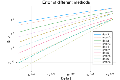
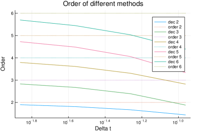
Refer to caption
Refer to caption
Figure 3: Second to sixth order error decay and slope of the errors

5.2 Nonlinear test problem

In this next subsection, we consider the nonlinear test problem

c1(t)superscriptsubscript𝑐1𝑡\displaystyle c_{1}^{\prime}(t) =c1(t)c2(t)c1(t)+1,absentsubscript𝑐1𝑡subscript𝑐2𝑡subscript𝑐1𝑡1\displaystyle=-\frac{c_{1}(t)c_{2}(t)}{c_{1}(t)+1}, (54)
c2(t)superscriptsubscript𝑐2𝑡\displaystyle c_{2}^{\prime}(t) =c1(t)c2(t)c1(t)+10.3c2(t),absentsubscript𝑐1𝑡subscript𝑐2𝑡subscript𝑐1𝑡10.3subscript𝑐2𝑡\displaystyle=\frac{c_{1}(t)c_{2}(t)}{c_{1}(t)+1}-0.3c_{2}(t),
c3(t)superscriptsubscript𝑐3𝑡\displaystyle c_{3}^{\prime}(t) =0.3c2(t)absent0.3subscript𝑐2𝑡\displaystyle=0.3c_{2}(t)

with initial condition 𝐜0=(9.98,0.01,0.01)Tsuperscript𝐜0superscript9.980.010.01𝑇\mathbf{c}^{0}=(9.98,0.01,0.01)^{T}. As before, this problem was proposed in [14]. The PDS system in the matrix formulation can be expressed by

p2,1(𝐜)=d1,2(𝐜)=c1(t)c2(t)c1(t)+1,p3,2(𝐜)=d2,3(𝐜)=0.3c2(t)formulae-sequencesubscript𝑝21𝐜subscript𝑑12𝐜subscript𝑐1𝑡subscript𝑐2𝑡subscript𝑐1𝑡1subscript𝑝32𝐜subscript𝑑23𝐜0.3subscript𝑐2𝑡p_{2,1}(\mathbf{c})=d_{1,2}(\mathbf{c})=\frac{c_{1}(t)c_{2}(t)}{c_{1}(t)+1},\quad p_{3,2}(\mathbf{c})=d_{2,3}(\mathbf{c})=0.3c_{2}(t)

and pi,j(𝐜)=di,j(𝐜)=0subscript𝑝𝑖𝑗𝐜subscript𝑑𝑖𝑗𝐜0p_{i,j}(\mathbf{c})=d_{i,j}(\mathbf{c})=0 for all other combinations of i𝑖i and j𝑗j. This system (54) is used to describe an algal bloom, that transforms nutrients c1subscript𝑐1c_{1} via phytoplankton c2subscript𝑐2c_{2} into detritus c3subscript𝑐3c_{3}. In our test, we consider the time interval [0,30]030[0,30] and Δt=0.5Δ𝑡0.5\Delta t=0.5. We calculate the reference solution with the strong stability preserving Runge-Kutta method 10 stages 4th order introduced by Ketcheson [13], further investigated in [22] and implemented in Julia, see [21] for details.
In Figure 4, the 6-th order mPDeC (black, dash-dotted lines) approximates very precisely the reference solution. The 2-nd order method (solid line, green) shows the same structure as the reference solution but it exhibits a severe error. However, the approximated second order solution is comparable with the results obtained in [14]. We see again that the conservation property is fulfilled in the purple lines.
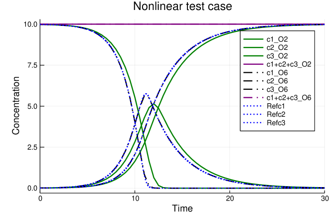
Refer to caption
Figure 4: Second order and sixth order methods together with the reference solution (SSPRK104)

Since we lack of an analytical solution, in the error plots, we compare successive errors between two refinements of the time mesh

EN=1Nn=1N(1Ii=1I(ci,Nnci,2N2n)2)12.subscriptE𝑁1𝑁superscriptsubscript𝑛1𝑁superscript1𝐼superscriptsubscript𝑖1𝐼superscriptsuperscriptsubscript𝑐𝑖𝑁𝑛superscriptsubscript𝑐𝑖2𝑁2𝑛212\mathrm{E}_{N}=\frac{1}{N}\sum_{n=1}^{N}\left(\frac{1}{I}\sum_{i=1}^{I}\left(c_{i,N}^{n}-c_{i,2N}^{2n}\right)^{2}\right)^{\frac{1}{2}}. (55)

Here, the subscript N𝑁N indicates the number of equispaced timesteps used to subdivide the total time interval. The results are presented in Figure 5. As for the linear case, we can see that the error decay fulfils the expected behavior and that the order of accuracy tends to the correct one. The slight decrease of the slope function in the right picture using sixth order can be explained by the fact that the error values are close to machine precision in that area and this causes the deprecation of the slope.

These plots verify our theoretical investigations from section 4.
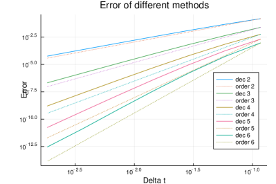
Refer to caption
Refer to caption
Figure 5: Second to sixth order error behaviors and slopes of the errors

5.3 Robertson Test case

In the last test case, we prove the robustness of the mPDeC schemes in presence of stiff problems. The proposed test is the Robertson problem for a chemical reaction system. It consists of

c1(t)superscriptsubscript𝑐1𝑡\displaystyle c_{1}^{\prime}(t) =104c2(t)c3(t)0.04c1(t)absentsuperscript104subscript𝑐2𝑡subscript𝑐3𝑡0.04subscript𝑐1𝑡\displaystyle=10^{4}c_{2}(t)c_{3}(t)-0.04c_{1}(t) (56)
c2(t)superscriptsubscript𝑐2𝑡\displaystyle c_{2}^{\prime}(t) =0.04c1(t)104c2(t)c3(t)3107c2(t)2absent0.04subscript𝑐1𝑡superscript104subscript𝑐2𝑡subscript𝑐3𝑡3superscript107subscript𝑐2superscript𝑡2\displaystyle=0.04c_{1}(t)-10^{4}c_{2}(t)c_{3}(t)-3\cdot 10^{7}c_{2}(t)^{2}
c3(t)superscriptsubscript𝑐3𝑡\displaystyle c_{3}^{\prime}(t) =3107c2(t)2absent3superscript107subscript𝑐2superscript𝑡2\displaystyle=3\cdot 10^{7}c_{2}(t)^{2}

with initial conditions 𝐜0=(1,0,0)superscript𝐜0100\mathbf{c}^{0}=(1,0,0).444To avoid the division by zero in the mPDeC scheme, we slightly modify the initial condition in the practical implementation, i.e., 𝐜0=(12eps,eps,eps)superscript𝐜012𝑒𝑝𝑠𝑒𝑝𝑠𝑒𝑝𝑠\mathbf{c}^{0}=(1-2eps,eps,eps) with eps=2.221016𝑒𝑝𝑠2.22superscript1016eps=2.22\cdot 10^{-16}. The time interval of interest is [106,1010]superscript106superscript1010[10^{-6},10^{10}]. The PDS for (56) reads

p1,2(𝐜)=d2,1(𝐜)=104c2(t)c3(t),p2,1(𝐜)=d1,2(𝐜)=0.04c1(t),p3,2(𝐜)=d2,3(𝐜)=3107c2(t)formulae-sequencesubscript𝑝12𝐜subscript𝑑21𝐜superscript104subscript𝑐2𝑡subscript𝑐3𝑡subscript𝑝21𝐜subscript𝑑12𝐜0.04subscript𝑐1𝑡subscript𝑝32𝐜subscript𝑑23𝐜3superscript107subscript𝑐2𝑡p_{1,2}(\mathbf{c})=d_{2,1}(\mathbf{c})=10^{4}c_{2}(t)c_{3}(t),\quad p_{2,1}(\mathbf{c})=d_{1,2}(\mathbf{c})=0.04c_{1}(t),\quad p_{3,2}(\mathbf{c})=d_{2,3}(\mathbf{c})=3\cdot 10^{7}c_{2}(t)

and zero for the other combinations.
In the Robertson test case, the numerical scheme has to deal with several time scales. Therefore, a constant time step size is not suitable for this purpose.
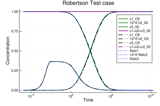
Refer to caption
Figure 6: Second and fifth order solutions and references

Following again the literature [14], we use increasing time steps Δtn=2n1Δt0Δsubscript𝑡𝑛superscript2𝑛1Δsubscript𝑡0\Delta t_{n}=2^{n-1}\Delta t_{0} with Δt0=106Δsubscript𝑡0superscript106\Delta t_{0}=10^{-6}, where n𝑛n indicates the n𝑛n-th timestep. To make the small c2subscript𝑐2c_{2} values visible on the plot, we multiply it by 104superscript10410^{4}. As a comparison, we calculate the reference solution (dotted, blue line) using the function Rodas4555 A 4-th order A-stable stiffly stable Rosenbrock method with a stiff-aware 3rd order interpolant. from Julia, where we split the time-interval into 55 subdomains and we solve it on every subdomain with relative tolerance 1020superscript102010^{-20} and absolute tolerance 1020superscript102010^{-20}. We plot again a second order (green, solid lines) and fifth order (black, dashed-dotted lines) approximations generated by the mPDeC methods and, as it can be seen in figure 6, the designed methods produce reliable and robust results for this kind of stiff problems. As always, the conservation and the positivity properties are fulfilled.

Finally, we can say that the simulations run in this section express the quality of the mPDeC schemes. Moreover, they show that all the targeted properties are obtained even for very problematic test cases.

6 Summary and Outlook

In this paper, we presented a way to build positivity preserving, conservative and arbitrary high-order numerical schemes for production-destructions systems of equations. We adapted the idea of [4] to build modified Patankar type schemes to the Deferred Correction method as an underlying scheme. By altering the 1superscript1\mathcal{L}^{1} and 2superscript2\mathcal{L}^{2} operators using the modified Patankar trick, we were able to obtain schemes with the desired properties. We proved that the proposed modified Patankar DeC (mPDeC) schemes are arbitrary high-order, conservative and positivity preserving. In numerical simulations, we confirmed our theoretical considerations with various test cases.
However, further research can be pursued in this direction. As it was investigated in [15, 14] for families of MPRK, it is possible to study the accuracy and the stability of the method varying the weightings of the production-destruction terms of the schemes. In the spirit of the work [14], a change of the weighting of the Patankar modification in the 1superscript1\mathcal{L}^{1} and 2superscript2\mathcal{L}^{2} operators should be easily applicable to the mPDeC schemes and theoretical investigations will be considered in future research, in particular regarding the stability conditions. Also the distribution of the subtimesteps between tnsuperscript𝑡𝑛t^{n} and tn+1superscript𝑡𝑛1t^{n+1} plays a big role on stability and accuracy of the scheme. Many choices are valid and the possible influence of the properties of the method must be carefully analysed. This idea is already work in progress for the classical DeC approach and will be extended to the mPDeC version in the future. Finally, we want to apply and analyse this type of schemes in context of partial differential equations. Here, we focus on applications and problems as described in [11, 12, 18]. As one can see, there are still many open questions and tasks for the mPDeC schemes and we are looking forward to continue our work in this field.

Appendix A Notation

We provide a small table 1 with the notation of symbols used along the paper. Even if some of the notations are ambiguous, the used indices should always clarify the referred meaning. We prefer to keep this notation to keep fluid the reading.

Notation Meaning
I𝐼I Number of constituents and dimension of the ODE system
i𝑖i Index for constituents
cisubscript𝑐𝑖c_{i} Value of the i𝑖ith constituents
𝐜𝐜\mathbf{c} Vector of all the constituents 𝐜=(c1,,cI)T𝐜superscriptsubscript𝑐1subscript𝑐𝐼𝑇\mathbf{c}=(c_{1},\dots,c_{I})^{T}
N𝑁N Number of time intervals
n𝑛n Index for a timestep
tnsuperscript𝑡𝑛t^{n} Timestep
𝐜nsuperscript𝐜𝑛\mathbf{c}^{n} Variables at timestep tnsuperscript𝑡𝑛t^{n}
M𝑀M Number of subtimeintervals in a timeinterval
m𝑚m Index for subtimesteps
tn,m=tmsuperscript𝑡𝑛𝑚superscript𝑡𝑚t^{n,m}=t^{m} Subtimestep
𝐜n,m=𝐜msuperscript𝐜𝑛𝑚superscript𝐜𝑚\mathbf{c}^{n,m}=\mathbf{c}^{m} Variable at subtimestep m𝑚m
𝐜¯¯𝐜\underline{\mathbf{c}} Vector of variables at all subtimestep m=0,,M𝑚0𝑀m=0,\dots,M
K𝐾K Number of iterations of the DeC procedure
(k)𝑘(k) Index of the iteration
𝐜n,m,(k)=𝐜m,(k)superscript𝐜𝑛𝑚𝑘superscript𝐜𝑚𝑘\mathbf{c}^{n,m,(k)}=\mathbf{c}^{m,(k)} Variables for timestep n𝑛n at the subtimestep m𝑚m and iteration k𝑘k
𝐜¯(k)superscript¯𝐜𝑘\underline{\mathbf{c}}^{(k)} Vector of variables for all subtimesteps m=0,,M𝑚0𝑀m=0,\dots,M at the iteration k𝑘k
1()superscript1\mathcal{L}^{1}(\cdot) First order operator of DeC procedure
2()superscript2\mathcal{L}^{2}(\cdot) High order operator of DeC procedure
2(,)superscript2\mathcal{L}^{2}(\cdot,\cdot) High order operator of mPDeC procedure
𝐜¯superscript¯𝐜\underline{\mathbf{c}}^{*} Solution of the system 2(𝐜¯)=0superscript2superscript¯𝐜0\mathcal{L}^{2}(\underline{\mathbf{c}}^{*})=0.
Table 1: Notation table

Appendix B Algorithm

We present a pseudo-code for the creation of the mass matrix in Algorithm 1 and one for the mPDeC algorithm in box Algorithm 2. Both algorithms are very simple. The first one consists of 3 loops: 2 for the constituents i,j=1,,Iformulae-sequence𝑖𝑗1𝐼i,j=1,\dots,I and one for the subtimesteps r=0,,M𝑟0𝑀r=0,\dots,M and an if statement. The second one consists of 3 nested loops: one for timesteps {tn}n=0Nsuperscriptsubscriptsuperscript𝑡𝑛𝑛0𝑁\{t^{n}\}_{n=0}^{N}, one for corrections of the DeC algorithm k=1,,K𝑘1𝐾k=1,\dots,K and one for the subtimesteps m=1,,M𝑚1𝑀m=1,\dots,M.

Algorithm 1 Mass
0:  Production-destruction functions pi,j(),di,j()subscript𝑝𝑖𝑗subscript𝑑𝑖𝑗p_{i,j}(\cdot),\,d_{i,j}(\cdot), previous correction variables 𝐜¯(k1)superscript¯𝐜𝑘1\underline{\mathbf{c}}^{(k-1)}, actual subtimestep m𝑚m.
1:  M:=0assignM0\mathrm{M}:=0
2:  for i=1𝑖1i=1 to I𝐼I do
3:     for j=1𝑗1j=1 to I𝐼I do
4:        for r=0𝑟0r=0 to M𝑀M do
5:           if θrm0superscriptsubscript𝜃𝑟𝑚0\theta_{r}^{m}\geq 0 then
6:              Mi,j=Mi,jΔtθrmpi,j(𝐜r,(k1))cjm,(k1)subscriptM𝑖𝑗subscriptM𝑖𝑗Δ𝑡superscriptsubscript𝜃𝑟𝑚subscript𝑝𝑖𝑗superscript𝐜𝑟𝑘1superscriptsubscript𝑐𝑗𝑚𝑘1\mathrm{M}_{i,j}=\mathrm{M}_{i,j}-\Delta t\theta_{r}^{m}\frac{p_{i,j}(\mathbf{c}^{r,(k-1)})}{c_{j}^{m,(k-1)}}
7:              Mi,i=Mi,i+Δtθrmdi,j(𝐜r,(k1))cim,(k1)subscriptM𝑖𝑖subscriptM𝑖𝑖Δ𝑡superscriptsubscript𝜃𝑟𝑚subscript𝑑𝑖𝑗superscript𝐜𝑟𝑘1superscriptsubscript𝑐𝑖𝑚𝑘1\mathrm{M}_{i,i}=\mathrm{M}_{i,i}+\Delta t\theta_{r}^{m}\frac{d_{i,j}(\mathbf{c}^{r,(k-1)})}{c_{i}^{m,(k-1)}}
8:           else
9:              Mi,j=Mi,j+Δtθrmdi,j(𝐜r,(k1))cjm,(k1)subscriptM𝑖𝑗subscriptM𝑖𝑗Δ𝑡superscriptsubscript𝜃𝑟𝑚subscript𝑑𝑖𝑗superscript𝐜𝑟𝑘1superscriptsubscript𝑐𝑗𝑚𝑘1\mathrm{M}_{i,j}=\mathrm{M}_{i,j}+\Delta t\theta_{r}^{m}\frac{d_{i,j}(\mathbf{c}^{r,(k-1)})}{c_{j}^{m,(k-1)}}
10:              Mi,i=Mi,iΔtθrmpi,j(𝐜r,(k1))cim,(k1)subscriptM𝑖𝑖subscriptM𝑖𝑖Δ𝑡superscriptsubscript𝜃𝑟𝑚subscript𝑝𝑖𝑗superscript𝐜𝑟𝑘1superscriptsubscript𝑐𝑖𝑚𝑘1\mathrm{M}_{i,i}=\mathrm{M}_{i,i}-\Delta t\theta_{r}^{m}\frac{p_{i,j}(\mathbf{c}^{r,(k-1)})}{c_{i}^{m,(k-1)}}
11:           end if
12:        end for
13:     end for
14:  end for
Algorithm 2 mPDeC
0:  Production-destruction functions pi,j(),di,j()subscript𝑝𝑖𝑗subscript𝑑𝑖𝑗p_{i,j}(\cdot),\,d_{i,j}(\cdot), timesteps {tn}n=0Nsuperscriptsubscriptsuperscript𝑡𝑛𝑛0𝑁\{t^{n}\}_{n=0}^{N}, initial condition 𝐜0superscript𝐜0\mathbf{c}^{0}.
1:  for n=1𝑛1n=1 to N𝑁N do
2:     for k=0𝑘0k=0 to K𝐾K do
3:        Set 𝐜0,(k):=𝐜nassignsuperscript𝐜0𝑘superscript𝐜𝑛\mathbf{c}^{0,(k)}:=\mathbf{c}^{n}
4:     end for
5:     for m=1𝑚1m=1 to M𝑀M do
6:        Set 𝐜m,(0):=𝐜nassignsuperscript𝐜𝑚0superscript𝐜𝑛\mathbf{c}^{m,(0)}:=\mathbf{c}^{n}
7:     end for
8:     for k=1𝑘1k=1 to K𝐾K do
9:        for m=1𝑚1m=1 to M𝑀M do
10:           Compute the mass matrix M(𝐜m,(k1)):=assignMsuperscript𝐜𝑚𝑘1absent\mathrm{M}(\mathbf{c}^{m,(k-1)}):=Mass(𝐜¯(k1),m)superscript¯𝐜𝑘1𝑚(\underline{\mathbf{c}}^{(k-1)},m) using algorithm 1
11:           Compute 𝐜m,(k)superscript𝐜𝑚𝑘\mathbf{c}^{m,(k)} solving the linear system M(𝐜m,(k1))𝐜m,(k)=𝐜nMsuperscript𝐜𝑚𝑘1superscript𝐜𝑚𝑘superscript𝐜𝑛\mathrm{M}(\mathbf{c}^{m,(k-1)})\mathbf{c}^{m,(k)}=\mathbf{c}^{n} given by (25)
12:        end for
13:     end for
14:     Set 𝐜n+1:=𝐜M,(K)assignsuperscript𝐜𝑛1superscript𝐜𝑀𝐾\mathbf{c}^{n+1}:=\mathbf{c}^{M,(K)}
15:  end for

Acknowledgements

P. Öffner has been funded by the the SNF project (Number 175784).
Davide Torlo is supported by ITN ModCompShock project funded by the European Union’s Horizon 2020 research and innovation program under the Marie Sklodowska-Curie grant agreement No 642768.

References

  • [1] R. Abgrall. High order schemes for hyperbolic problems using globally continuous approximation and avoiding mass matrices. Journal of Scientific Computing, 73(2):461–494, Dec 2017.
  • [2] R. Abgrall, E. l. Meledo, and P. Öffner. On the connection between residual distribution schemes and flux reconstruction. arXiv preprint arXiv:1807.01261, 2018.
  • [3] R. Abgrall and D. Torlo. Asymptotic preserving deferred correction residual distribution schemes. arXiv preprint arXiv:1811.09284, 2018.
  • [4] H. Burchard, E. Deleersnijder, and A. Meister. A high-order conservative patankar-type discretisation for stiff systems of production–destruction equations. Applied Numerical Mathematics, 47(1):1–30, 2003.
  • [5] H. Burchard, E. Deleersnijder, and A. Meister. Application of modified patankar schemes to stiff biogeochemical models for the water column. Ocean Dynamics, 55(3-4):326–337, 2005.
  • [6] A. Christlieb, B. Ong, and J.-M. Qiu. Integral deferred correction methods constructed with high order runge-kutta integrators. Mathematics of Computation, 79(270):761–783, 2010.
  • [7] A. Dutt, L. Greengard, and V. Rokhlin. Spectral Deferred Correction Methods for Ordinary Differential Equations. BIT Numerical Mathematics, 40(2):241–266, 2000.
  • [8] S. Gottlieb, D. I. Ketcheson, and C.-W. Shu. Strong stability preserving Runge-Kutta and multistep time discretizations. World Scientific, 2011.
  • [9] E. Hairer, S. P. Nørsett, and G. Wanner. Solving ordinary differential equations. 1, Nonstiff problems. Springer-Vlg, 1991.
  • [10] I. Hense and A. Beckmann. The representation of cyanobacteria life cycle processes in aquatic ecosystem models. Ecological Modelling, 221(19):2330–2338, 2010.
  • [11] J. Huang and C.-W. Shu. Positivity-preserving time discretizations for production–destruction equations with applications to non-equilibrium flows. Journal of Scientific Computing, 78(3):1811–1839, 2019.
  • [12] J. Huang, W. Zhao, and C.-W. Shu. A third-order unconditionally positivity-preserving scheme for production–destruction equations with applications to non-equilibrium flows. Journal of Scientific Computing, pages 1–42, 2018.
  • [13] D. I. Ketcheson. Highly efficient strong stability-preserving Runge-Kutta methods with low-storage implementations. SIAM Journal on Scientific Computing, 30(4):2113–2136, 2008.
  • [14] S. Kopecz and A. Meister. On order conditions for modified patankar–runge–kutta schemes. Applied Numerical Mathematics, 123:159–179, 2018.
  • [15] S. Kopecz and A. Meister. Unconditionally positive and conservative third order modified patankar–runge–kutta discretizations of production–destruction systems. BIT Numerical Mathematics, pages 1–38, 2018.
  • [16] S. Kopecz and A. Meister. On the existence of three-stage third-order modified patankar–runge–kutta schemes. Numerical Algorithms, pages 1–12, 2019.
  • [17] Y. Liu, C.-W. Shu, and M. Zhang. Strong stability preserving property of the deferred correction time discretization. Journal of Computational Mathematics, pages 633–656, 2008.
  • [18] A. Meister and S. Ortleb. On unconditionally positive implicit time integration for the dg scheme applied to shallow water flows. International Journal for Numerical Methods in Fluids, 76(2):69–94, 2014.
  • [19] M. L. Minion. Semi-implicit spectral deferred correction methods for ordinary differential equations. Commun. Math. Sci., 1(3):471–500, 09 2003.
  • [20] S. Patankar. Numerical heat transfer and fluid flow. CRC press, 1980.
  • [21] C. Rackauckas and Q. Nie. Differentialequations. jl–a performant and feature-rich ecosystem for solving differential equations in julia. Journal of Open Research Software, 5(1), 2017.
  • [22] H. Ranocha and P. Öffner. L2subscript𝐿2L_{2} stability of explicit Runge-Kutta schemes. Journal of Scientific Computing, 75(2):1040–1056, 05 2018.
  • [23] H. Ranocha, P. Öffner, and T. Sonar. Summation-by-parts operators for correction procedure via reconstruction. Journal of Computational Physics, 311:299–328, 2016.
  • [24] G. Wanner and E. Hairer. Solving ordinary differential equations II. Springer Berlin Heidelberg, 1996.