Separating Overlapping Tissue Layers from Microscopy Images

Abstract

Manual preparation of tissue slices for microscopy imaging can introduce tissue tears and overlaps. Typically, further digital processing algorithms such as registration and 3D reconstruction from tissue image stacks cannot handle images with tissue tear/overlap artifacts, and so such images are usually discarded. In this paper, we propose an imaging model and an algorithm to digitally separate overlapping tissue data of mouse brain images into two layers. We show the correctness of our model and the algorithm by comparing our results with the ground truth.

Index Terms—  Overlaid artifact, image separation, texture synthesis, Microscopy imaging model, overlapping images

1 Introduction

Tissues of mouse brain images sliced for the purpose of neuron tracing and high resolution digital 3D brain reconstruction, are too thin for robust manual handling [1, 2]. At the time the tissues are laid on the glass for imaging, there can be tissue tears and tissue overlaps. Images of such tissues are typically discarded before further digital processing of tissue image stacks since almost none of the algorithms down the pipeline will be able to handle such artifacts. In this paper, we propose how missing regions of two overlaid tissue layers can be reconstructed using texture synthesis.

There have been previous works on repairing tissue damage artifacts. However, these earlier works paid attention to some of the other microscopy image artifacts. For instance, [3] explored dust air bubbles and particles. Tissue deformations such as stretching and compaction have been addressed in [4]. Moreover, blind separation approach has become popular for separation of two independent overlapping images that have completely different components [5, 6]. Obviously, it fails on separating overlapping tissue layers of a single microscopy image that has same components. Also, same approach is used for denoising medical images in [7]. Furthermore, in our recent work [8, 9], we developed robust registration algorithm to handle images with tissue tears or with missing tissue data. However, tissue overlap artifact handling is still an open problem and is addressed in this article.

Fig. 1: Imaging model with respect to the microscope capturing process. L is the incoming light, $X$ and $Y$ are the reflection coefficients for two overlapping tissue layers $T_{1}$ and $T_{2}$, respectively.

2 Proposed Method

In this section, we propose a method to separate two overlapping tissues in digital images into two layers. The input to our method, is the section of the digital microscopy image that has two-tissue overlap as well as some part outside the overlap region. Using known information in the non-overlapping neighborhoods of the overlapping region and the imaging model, two individual tissue layers are computed and separated. The outputs of our method are two digitally separated tissue layers.

2.1 Texture Synthesis

the information from adjacent non-overlapping neighborhood of the boundary of the overlaps provide the initialization data to start the optimization process of reconstructing the individual tissue layers. We use one of the hole filling methods [10, 11], PatchMatch [12], to initialize the two tissue layers. Following the initialization, the content of each tissue layer is iteratively optimized so that a virtual image of the overlap of the two reconstructed layers matches with the real input image of the overlapping region. We also propose a microscope imaging model in order to capture a virtual image.

2.2 Imaging Model

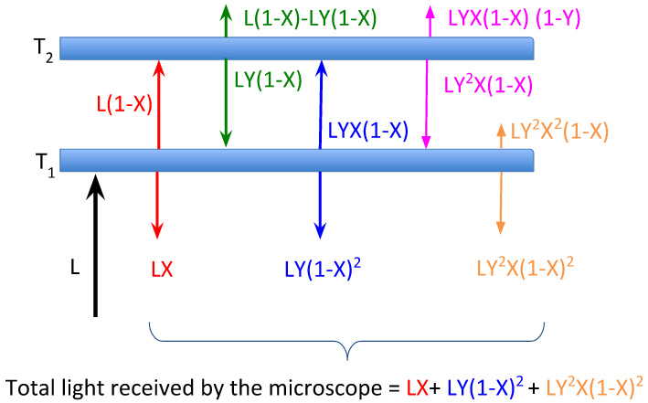
We propose an imaging model to specifically express the overlapping tissue capturing process. Using this model, we virtually capture the digital overlap of the separated output tissues and compare it with the original captured overlaid region to evaluate the results. The imaging model is illustrated in Figure 1 where L is the incoming light, $X$ and $Y$ are the reflection coefficients for the two overlapping tissue layers $T_{1}$ and $T_{2}$, respectively. $X$ and $Y$ are initialized using texture synthesis methods discussed in Section 2.1. They should be updated such that the obtained output $Z$ after applying the imaging model, would be the closest value at that particular pixel in the original overlaid area, cropped from the input. If $Z$ is the total light received by the microscope, then regarding to Figure 1:

$$Z=X+Y(1-X)^{2}+XY^{2}(1-X)^{2}$$ (1)

The two assumptions of our imaging model of overlapping tissue is that the intensity of the source light $L$ is one, and the amount of light absorbed by the tissue is zero. In other words, the incoming light is equal to the sum of the reflected and transmitted light by the tissue. It is worth mentioning that we applied the model just for two paths of bouncing, and we assume that the light that is not accounted for is negligible.

2.3 Regularization

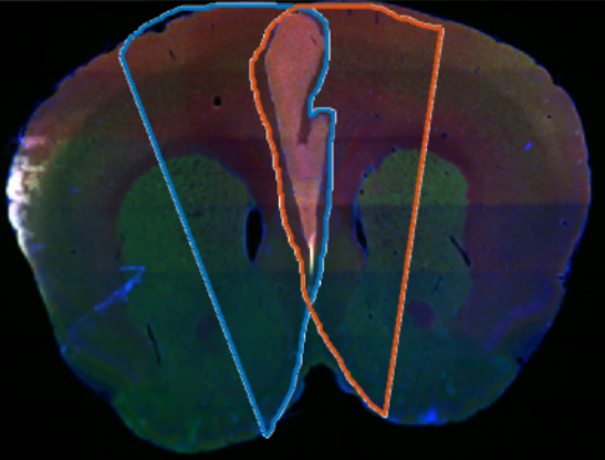
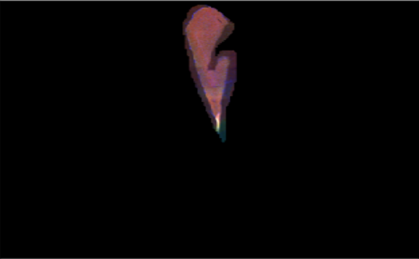
The initialized $X$ and $Y$ produced in Section 2.2 can be tuned in order to minimize the error which is defined as the Mean Square Error (MSE) between the obtained virtual imaging of the overlaid region $Z$ from Equation 1 and the input original image of the overlaid region $Z^{\prime}$. $Z$ and $Z^{\prime}$ are displayed in Figure 3 (b) and (c). For this purpose, two weights are used to update the current $X$ and $Y$ according to Equation 2.

$$X=X\times{W_{1}}\quad\textrm{and}\quad Y=Y\times{W_{2}}$$ (2)

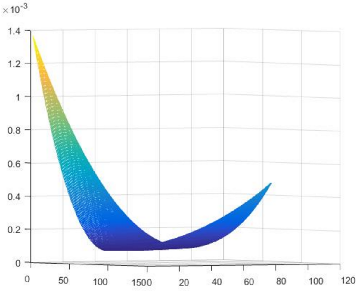
The corresponding error $Z-Z^{\prime}$ is calculated for every possible pair of updated $X$ and $Y$ in terms of all $W_{1}$ and $W_{2}$ in the range of $01$ represented in Figure 2. The optimum $X$ and $Y$ are obtained using gradient descent which is discussed in Section 2.3.1.

Fig. 2: Error surface corresponding to a pair of weights for both engaging tissue layers

2.3.1 Gradient Descent Optimization

In order to find the optimum $X$ and $Y$, we use gradient descent with the objective function $G$ visualized in Figure 2. The gradient of $G$ with respect to $X$ and $Y$ are calculated as follows according to Equation 1. The $X$ and $Y$ values are updated until the error is within the threshold $\epsilon$.

$$G=min\sum_{i=1}^{n}\sum_{j=1}^{m}(Z_{ij}-Z^{\prime}_{ij})^{2}$$

$$\nabla{G}=[\frac{\partial{G}}{\partial{x_{11}}},\frac{\partial{G}}{\partial{x_{12}}},\ldots,\frac{\partial{G}}{\partial{x_{nm}}},\frac{\partial{G}}{\partial{y_{11}}},\frac{\partial{G}}{\partial{y_{12}}},\ldots,\frac{\partial{G}}{\partial{y_{nm}}}]$$

$$\partial{G}/\partial{x_{ij}}=1-2(1-x_{ij})y_{ij}-2x_{ij}(1-x_{ij})y_{ij}^{2}+(1-x_{ij})^{2}y_{ij}^{2}$$

$$\partial{G}/\partial{y_{ij}}=(1-x_{ij})^{2}+2x_{ij}(1-x_{ij})^{2}y_{ij}$$

$$X_{t}=X_{t-1}-\alpha\nabla{G}\quad\textrm{and}\quad Y_{t}=Y_{t-1}-\alpha\nabla{G}$$

$$|G(X_{t})-G(X_{t-1})|<\epsilon\quad\textrm{and}\quad|G(Y_{t})-G(Y_{t-1})|<\epsilon$$

(a) Input image with overlap artifact

(b) Original overlaid area $Z^{\prime}$

(c) Obtained overlaid area $Z$

Fig. 3: The error is defined by the MSE between (b) and (c).

(a)

(b)

(c)

(d)

(e)

(f)

(g)

(h)

(i)

(j)

(k)

(l)

Fig. 4: A sample of three mouse brain slices with overlaid artifact and the overlapping contours depicted by the user are shown in the first row. Cropped recovered region for the right and left side of the damaged tissue within their contours are shown in the second and third row, respectively. Last row represents the separated corresponding contours on the ground truth images.

(a) Obtained right tissue layer

(b) Ground truth for the right tissue

(c) Obtained left tissue layer

(d) Ground truth for the left tissue

Fig. 5: Visual evaluation of the reconstructed tissue layers with the corresponding contour in the ground truth image achieved by recapturing damaged slices for the first sample in Figure 4.

2.4 Implementation and Experiment

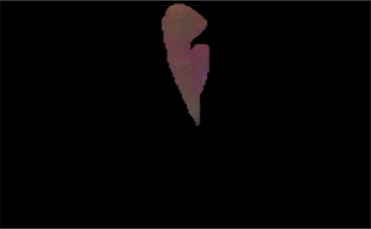
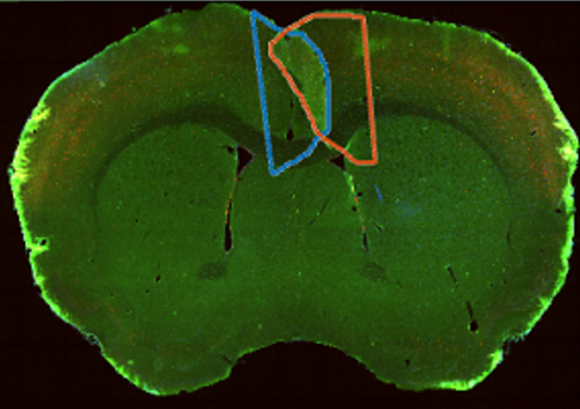
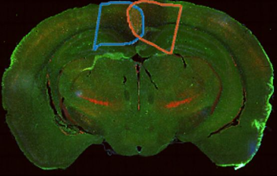
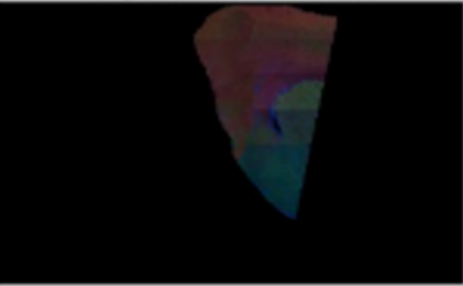
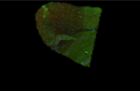
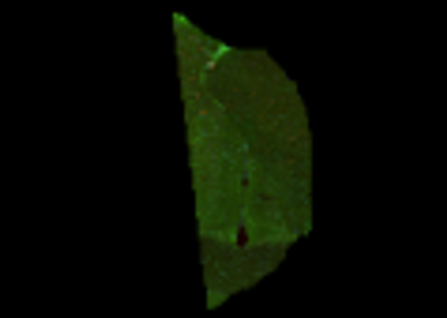
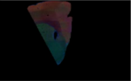
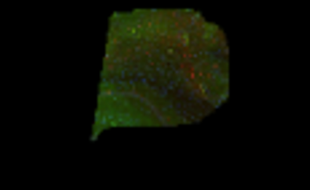
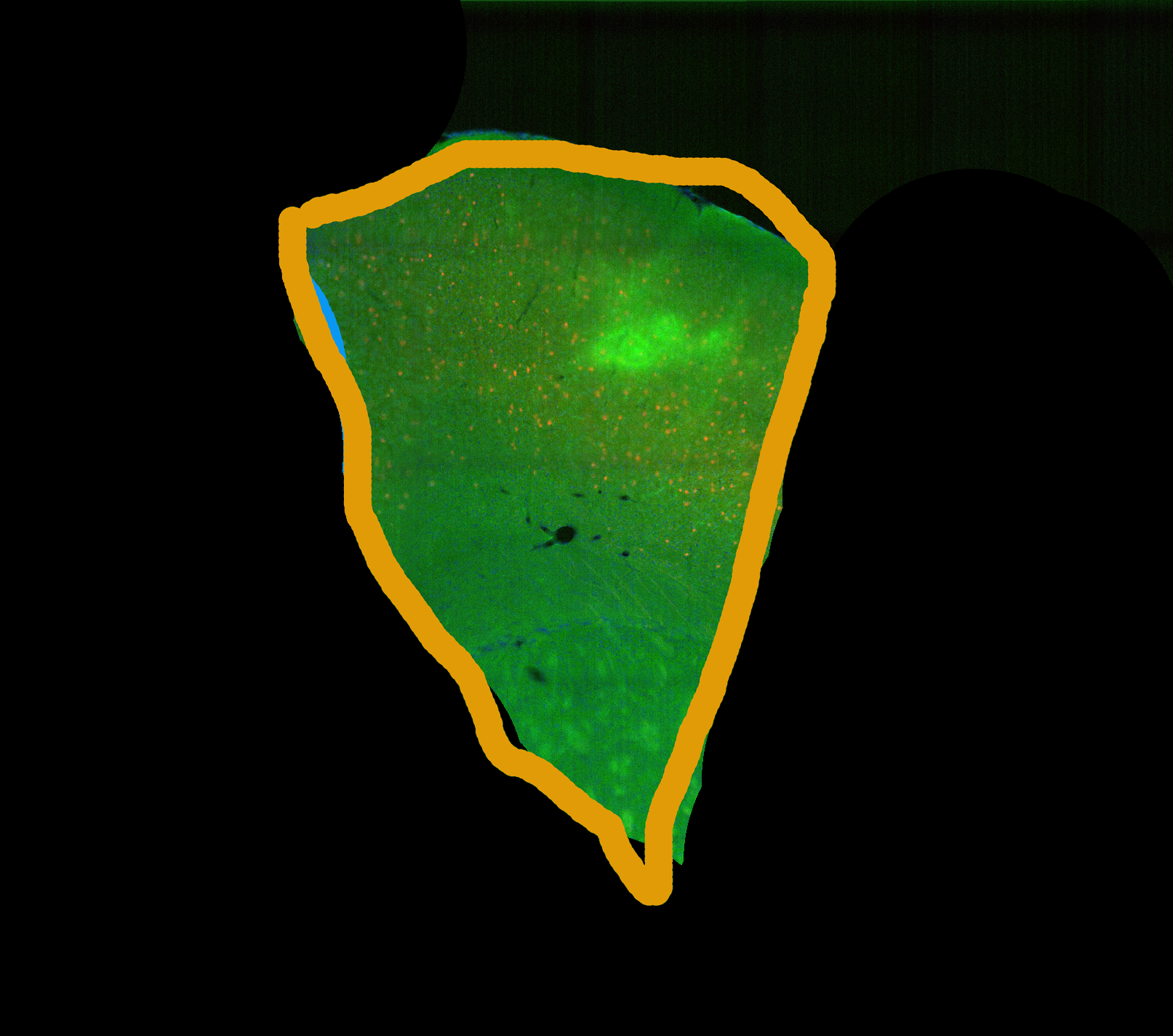
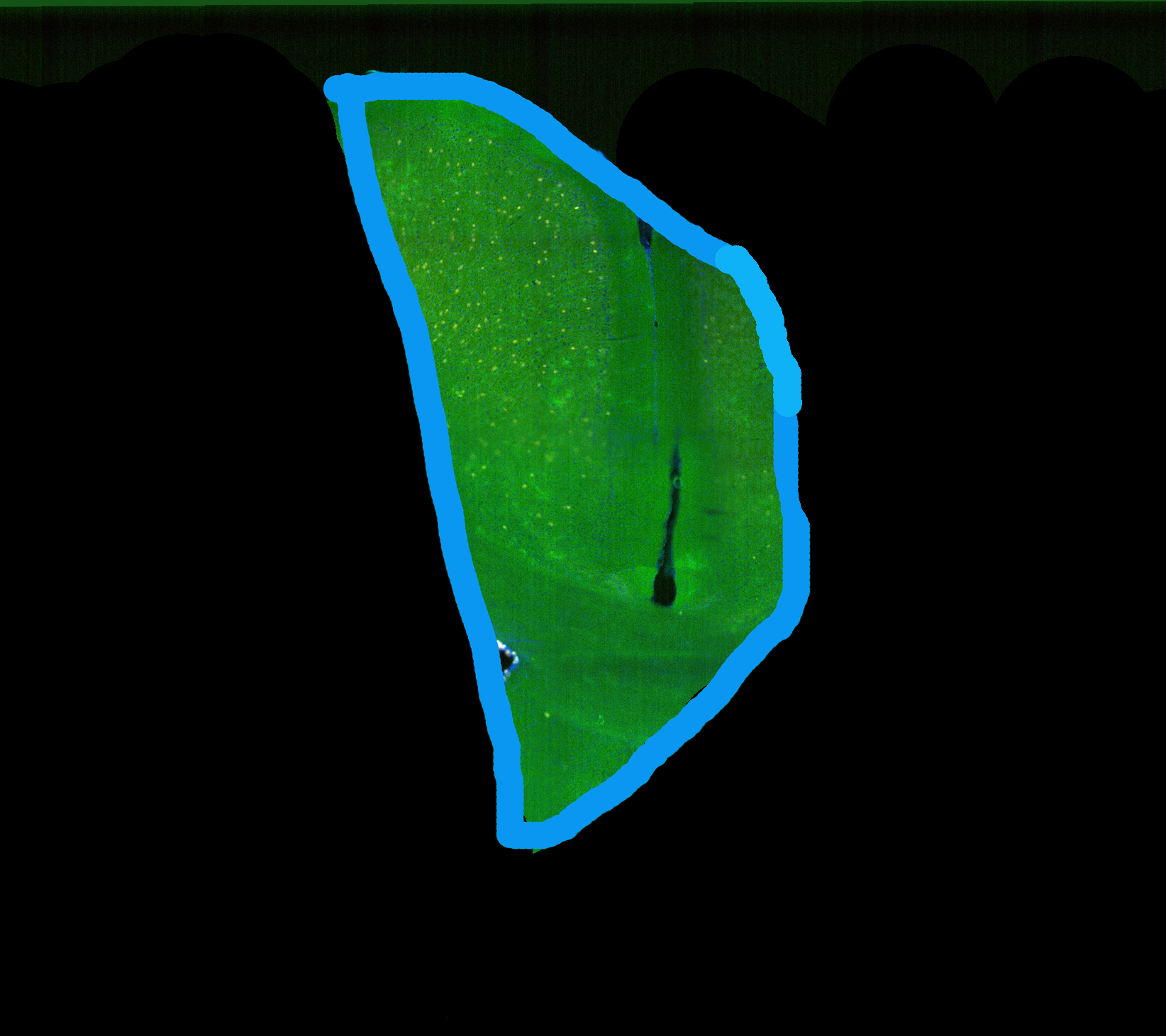
The code is implemented in Matlab and covers all the aforementioned steps in this section. Here is an overview of analysis pipeline illustrated in Figures 3 and 4. The input to our method presented in Figure 3 image (a). The overlaid region is shown brighter, which is expected and predicted by the proposed imaging model. In the middle image the original overlaid region of the two tissue layers is depicted. This is used as the ground truth for regularization section as well as optimization step to be compared with the obtained $Z$ displayed in image (c). As it is discussed in Section 2.1, first, Patch-Match algorithm applied. Then, the regularization step is performed addressed in Section 2.3. In Figure 2, the error for different pair of weights are visualized in 3D. The chart illustrates how the error is changed over the different values. The weights yielding the minimum error are picked for the rest of the pipeline using gradient descent optimization, covered in Section 2.3.1. The iteration stops when the error between the computed and the goal drops below a defined tolerance. The second and third row of Figure 4 demonstrate the final results after separating the overlaid tissue layers.

3 Results and Evaluation

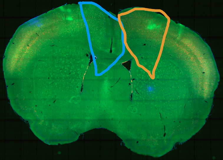
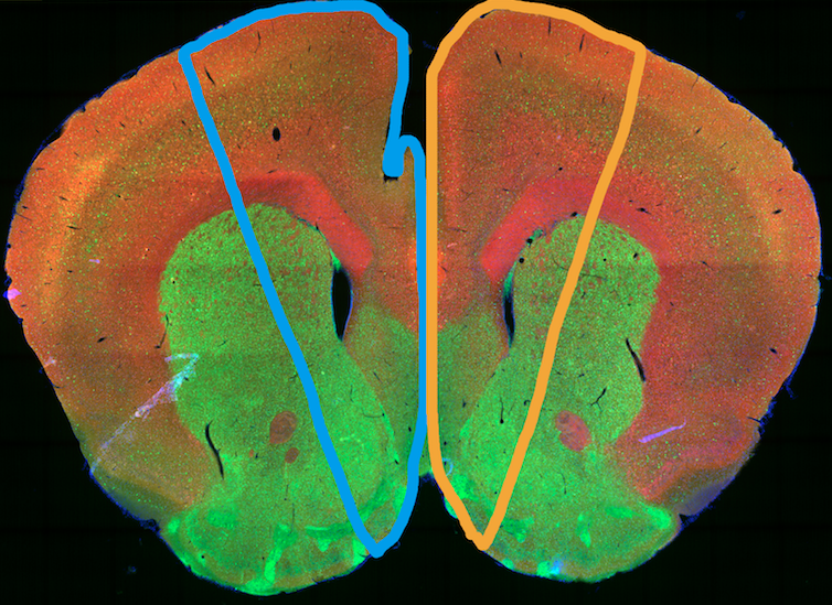
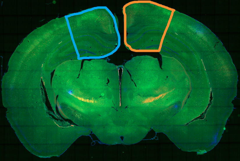
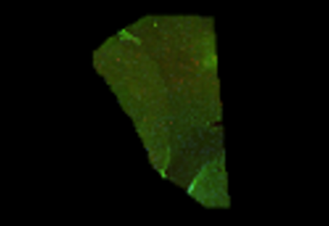
Our method provides two separated tissue layers as an output after employing the aforementioned steps. The final results of three samples with overlapping artifact are shown in Figure 4. In the first row. Results for the reconstructed right and left side of the damaged tissue within their contours are shown in the second and third row, respectively. Most importantly, just for evaluating the proposed microscopy image capture model, we physically separated the tissue slices and recaptured the microscopy images of these separated layers, and compared the new image with the layers of tissue separated by our algorithm. This is represented in the last row. Due to new stretching and contraction of tissues, the new slice will not have pixel to pixel correspondence with the old slice that has overlapping tissue layers. So the evaluation of the correctness of our result is only visual.
Figure 5 expresses the comparison between the obtained results for the two engaging tissue layers and the ground truth which is achieved by recapturing the slice and registering the corresponding regions. The results are from the first sample shown in Figure 4. Recapturing process produces different illumination and a slight changes in orientation due to manual interaction with the slice. Therefore, the ground truth image looks brighter and stretched than the obtained result. According to the results we tested for many samples, it is shown that the overall behavior of the texture has been reconstructed perfectly.

4 Future Work and Conclusion

One of the important plausible works is to extend the method to support the tissues that are folded multiple times. For this purpose, a new imaging model must be proposed depending on the number of overlapping tissues. Then, we can start with the initialization using texture synthesis as before, but one side of known region must be used for estimating the missing data each time. For the next unknown region, the obtained information for the previous unknown area can be used and similarly, the value for the following region will be needed for obtaining the further layers. Obviously, the more folded layers, the less accurate our method would performs.
Another potential direction of future research would be to estimate two indicated contours automatically instead of the user manipulation that we already have. As it mentioned in Section 3, the overlaid region is the brightest area in the tissue which is perceivable by considering the proposed imaging model. Therefore, the overlaid region can be detected automatically. Adequate known neighbor regions are also needed for both sides of the tissue. Having these three regions, one for the bright overlaid region, another two for depicting two neighborhoods, we are all set to pursue the rest of the pipeline.

5 Conclusion

This article proposes a microscopy imaging model for two layer tissue overlap and an efficient end-to-end pipeline for digital separation of overlaid tissues in microscopy images. We have demonstrated the successful results of the two separated tissues after applying our model comparing with the ground truth. We first start with a hole-filling technique, described in Section 2.1, as an initialization for the two tissue layers. Then we apply regularization step, discussed in Section 2.3. Then, an optimization technique is applied to obtain the optimum values for both sides with respect to the defined objective function. This step has been described in Section 2.3.1. Section 3 evaluates the results by comparing them with the ground truth.

6 Acknowledgement

The authors would like to thank Xiaoxiao Lin for providing the mouse brain images.

References

- [1] Hanchuan Peng, “Bioimage informatics: a new area of engineering biology,” Bioinformatics, vol. 24, no. 17, pp. 1827–1836, 2008.
- [2] Leonard Kuan, Yang Li, Chris Lau, David Feng, Amy Bernard, Susan M Sunkin, Hongkui Zeng, Chinh Dang, Michael Hawrylycz, and Lydia Ng, “Neuroinformatics of the allen mouse brain connectivity atlas,” Methods, vol. 73, pp. 4–17, 2015.
- [3] LM Kindle, IA Kakadiaris, T Ju, and JP Carson, “A semiautomated approach for artefact removal in serial tissue cryosections,” Journal of microscopy, vol. 241, no. 2, pp. 200–206, 2011.
- [4] Tao Ju, Joe Warren, James Carson, Musodiq Bello, Ioannis Kakadiaris, Wah Chiu, Christina Thaller, and Gregor Eichele, “3d volume reconstruction of a mouse brain from histological sections using warp filtering,” Journal of Neuroscience Methods, vol. 156, no. 1, pp. 84–100, 2006.
- [5] Anthony J Bell and Terrence J Sejnowski, “An information-maximization approach to blind separation and blind deconvolution,” Neural computation, vol. 7, no. 6, pp. 1129–1159, 1995.
- [6] E. Be’ery and A. Yeredor, “Blind separation of superimposed shifted images using parameterized joint diagonalization,” IEEE Transactions on Image Processing, vol. 17, no. 3, pp. 340–353, March 2008.
- [7] A. Mustafi and S.K. Ghorai, “A novel blind source separation technique using fractional fourier transform for denoising medical images,” Optik - International Journal for Light and Electron Optics, vol. 124, no. 3, pp. 265–271, 2013.
- [8] Nitin Agarwal, Xiangmin Xu, and M. Gopi, “Robust registration of mouse brain slices with severe histological artifacts,” in Proceedings of the Tenth Indian Conference on Computer Vision, Graphics and Image Processing. 2016, ICVGIP ’16, p. 10, ACM.
- [9] Nitin Agarwal, Xiangmin Xu, and M. Gopi, “Automatic detection of histological artifacts in mouse brain slice images,” in International MICCAI Workshop on Medical Computer Vision. Springer, 2016, p. TBD.
- [10] Alexei A. Efros and Thomas K. Leung, “Texture synthesis by non-parametric sampling,” in Proceedings of the International Conference on Computer Vision-Volume 2 - Volume 2, Washington, DC, USA, 1999, ICCV ’99, pp. 1033–, IEEE Computer Society.
- [11] Soheil Darabi, Eli Shechtman, Connelly Barnes, Dan B Goldman, and Pradeep Sen, “Image melding: Combining inconsistent images using patch-based synthesis.,” ACM Trans. Graph., vol. 31, no. 4, pp. 82–1, 2012.
- [12] Connelly Barnes, Eli Shechtman, Adam Finkelstein, and Dan B Goldman, “PatchMatch: A randomized correspondence algorithm for structural image editing,” ACM Transactions on Graphics (Proc. SIGGRAPH), vol. 28, no. 3, Aug. 2009.