WPU-Net: Boundary Learning by Using Weighted Propagation in Convolution Network

Abstract

Deep learning has driven a great progress in natural and biological image processing. However, in material science and engineering, there are often some flaws and indistinctions in material microscopic images induced from complex sample preparation, even due to the material itself, hindering the detection of target objects. In this work, we propose WPU-net that redesigns the architecture and weighted loss of U-Net, which forces the network to integrate information from adjacent slices and pays more attention to the topology in boundary detection task. Then, the WPU-net is applied into a typical material example, i.e., the grain boundary detection of polycrystalline material. Experiments demonstrate that the proposed method achieves promising performance and outperforms state-of-the-art methods. Besides, we propose a new method for object tracking between adjacent slices, which can effectively reconstruct 3D structure of the whole material. Finally, we present a material microscopic image dataset with the goal of advancing the state-of-the-art in image processing for material science.

Microstructure is crucial for controlling the properties and performance in material science (?). And during quantitative analysis of that, an important step is microscopic image processing, which is used for extracting the key information.

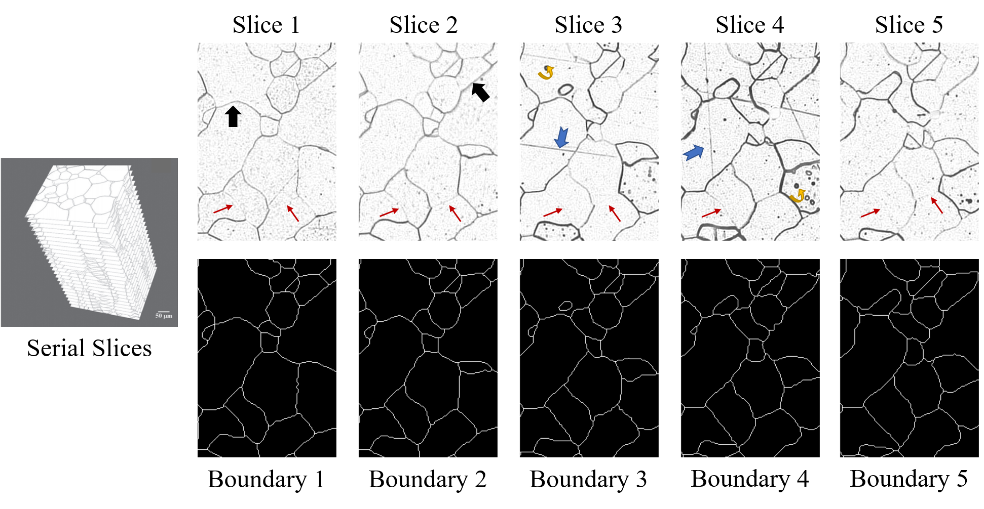
Unlike the image processing task in natural and biological scenes, the microscopic image in material science has its unique problems, which increase the difficulty of image processing and analyzing. Take microstructure analysis of polycrystalline iron for example, the ultimate objective is to obtain the 3D structure of the sample. Due to the opacity of materials, researchers can only use serial section method to obtain serial 2D slices (images) and stack it to reconstruct 3D structure, shown in Figure 1. Thus, there are two important steps in the process: 2D image analysis and 3D reconstruction. Both of them have their own difficulty.

For 2D image analysis, flaws in material microscopic images seriously hinder the target object detection (?). The region of interest in polycrystalline microscopic images is the single-pixel closed boundary of grain (like a cell in biological image) (?), as shown with black straight and thick arrows in Figure 1. Unfortunately, during sample preparation, such as polish and etch processes, the sample will unavoidably produce flaws. There are three types of flaws in polycrystalline microscopic images, which will pose significant problems for boundary detection task.

• Blurred or missing boundary: caused by incomplete etching in the nital solution, as shown with red straight and thin arrows. This kind of flaw may occur in any position of slices, even in the same position of serial slices. It is necessary for an algorithm to recover them correctly.

• Noise: caused in sample preparation, as shown with yellow curved arrows.

• Spurious scratch: unavoidably caused in polished process, which looks similar to the boundary and tends to confuse the image processing algorithm, as shown with blue notched arrows.

Figure 1: Microscopic serial slices of polycrystalline iron. The left is the demonstration of serial slices. The right top is five serial raw slices and its corresponding boundary results at right bottom. For interpretation of the references to color in this figure legend, the reader is referred to the web version of the article.

Attribute to high representative model, convolution neural networks(CNN) has driven a great success on image segmentation (?) and boundary detection (?) in recent years. However, as far as we know, there is no deep learning-based method specially designed for polycrystalline structural materials with such kind of flaws.

For 3D reconstruction, it is a challenge to identify the same grain regions in adjacent slices. Different degrees of deformation exists in the same grain between adjacent slices. In addition, grain disappearance and appearance often occur in slices. Therefore, it is necessary to design an algorithm which can solve all these problems when transforming 2D boundary detection images to 3D label result.

In this work, to solve the problem existed in 2D microscopic images of polycrystalline materials, we propose a novel Weighted Propagation Convolution Neural Network based on U-Net(WPU-Net), which propagates boundary information from adjacent slice to aid the boundary detection in the target slice.

Our work presents four contributions and our code and data are available in https://github.com/clovermini/WPU-Net.

• We propose an adaptive boundary weighted loss to force the network to tolerate minor difference in boundary location and pay more attention to topology preservation.

• We modify u-net by introducing 3D information into U-net architecture, which makes better use of domain knowledge between slices.

• We propose a new solution to reconstruct the 3D structure of sample by using CNN to perform grain object tracking between slices.

• We present a dataset with the goal of advancing the state-of-the-art in image processing for materials sciences.

Related work

Boundary Detection

Many existing methods have been used to detect the boundary of 3D polycrystalline material microscopic images. They can be broadly categorized into two classes: 2D image-based and 3D image-based methods, according to the input of method.

For 2D image-based, Deep Learning based methods (?; ?) for 2D semantic segmentation have become the de facto standard by virtue of its powerful feature learning and expression ability. The U-Net (?) is one of the most commonly used methods as its excellent performance. Many improved methods (?; ?) including ours are based on it. However, the 2D image-based methods have an inherent drawback, that is, it can not make use of the 3D context information between adjacent slices.

The 3D image-based methods can also be broadly grouped into three classes based on how to use 3D information. (I) 3D fully convolution network(FCN) (?; ?), which employs 3D convolution to replace 2D convolution. 3D U-Net (?) and V-Net (?) are the two most representative methods. (II) Combining 2D FCN with RNN. A representative method is UNet+BDCLSTM (?), which uses 2D FCN to extract intra-slice contexts, and recurrent neural network (RNN) to analyze inter-slice contexts. (III) Tracking-based method. (?) developed an interactive segmentation method based on break-point detection, but a lot of artificial correction is needed. (?) proposed the concept ”propagation segmentation” based on graph-cut, it sets the energy function of the target image with information of last slice. (?) improved the setting of binary terms in energy function, filling the blurred or missing boundary in target images with the same boundary in last slice. The tracking-based methods show superior performance when dealing with blurred or missing boundaries and spurious scratches. However, they are usually designed by hand-crafted features which is very time consuming. Our method combines the deep learning-based architecture with tracking-based method to take advantage of both, achieving the promising performance in comparison with state-of-the-art methods.

Weighted Loss

Weighted loss is widely used to handle the class imbalance problem in deep learning, weighted cross-entropy for example (?). However, it does not tolerate minor differences in boundary location. U-net (?) has proposed a weighted map loss to pay more attention to the border of two objects. However, it can only be applied to loosely arranged regions. Besides, it will be equal to weighted cross-entropy when applied to tightly arranged regions.

3D Reconstruction

There are two classes of 3D reconstruction methods to recognize the same regions in adjacent slices. The segmentation based, such as 3D watershed (?), uses distance information or gradient information to determine the relationship between two adjacent pixels. Unfortunately, the polycrystalline structure is complex and staggered, the grain region in one slice is connected to other grains in voxel relation on adjacent slices so that the 3D watershed cannot be applied to this task. The track based methods calculate shape similarity and overlap area between two connected components in two adjacent slices (?). However, both of them rely on hand-crafted features which will unavoidably cause the over-segment problem.

Method

Adaptive Boundary Weighted Map

Traditional weighted cross-entropy rigidly controls the location of the predicted boundary at pixel level. However, in a practical point, the topology of grain and boundary is what truly focused. U-net (?) has proposed a weighted map to force the network to learn the separation borders between two regions. This is very suited to loosely arranged regions. However, for tightly arranged regions, $d_{1}$ and $d_{2}$ are equals to 0 and the result is same with weighted cross-entropy.

By getting inspiration from U-net, an adaptive boundary weighting method is proposed, which is a weighted map incorporated with cross entropy calculation. The formulas are shown as below:

$$E=-\sum_{x\in\Omega}loss\_term(x)$$ (1)

$$loss\_term(x)=$$ (2)

$$\begin{cases}w_{bck}(x)\times log(p_{0}(x)),&\mbox{if }w_{bck}(x)\geq w_{obj}(x)\times m_{d}(x)\\ w_{obj}(x)\times log(p_{1}(x)),&\mbox{if }w_{bck}(x)<w_{obj}(x)\times m_{d}(x)\end{cases}$$

$$w_{bck}(x)=w_{c}(x)+w_{0}\times exp(-\frac{(max\_dis_{i}-d(x))^{2}}{2\times\sigma_{i}^{2}})$$ (3)

$$w_{obj}(x)=w_{c}(x)+w_{0}\times exp(-\frac{d(x)^{2}}{2\times\sigma_{i}^{2}})$$ (4)

$$\sigma_{i}=\frac{max\_dis_{i}}{\gamma}$$ (5)

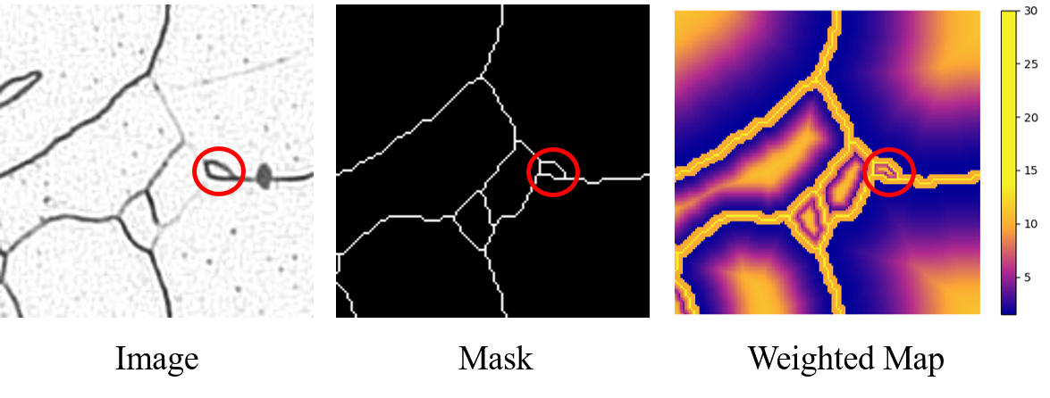
$E$ is the loss function computed by a pixel-wise soft-max over the final feature map combined with the cross-entropy function. The soft-max is defined as $p_{k}(x)=\frac{exp(a_{k}(x))}{\sum_{k^{\prime}}^{K}exp(a_{k^{\prime}}(x))}$ where $a_{k}(x)$ denotes the activation in feature channel $k$ at the pixel position $x$. $K$ is equal to the number of classes. $w_{c}(x)$ is the weighted map to balance the class frequencies. We design two types of weights, $w_{bck}(x)$ and $w_{obj}(x)$, for background and object respectively. For each pixel $x$ in grain $i$, we calculate its distance $d(x)$ to the nearest boundary and get the maximum of $d(x)$ in grain $i$, the $max\_dis_{i}$. We customize the weight for each grain by using $max\_dis_{i}$ in the above formulas. By making such optimization, the algorithm adaptively control the convergence speed of normal function. The smaller the grain size, the faster the weight converge, which protects the tiny grain and tolerate minor differences in boundary location. $m_{d}$ is the dilating result of the single-width mask which controls the range of variation of the boundary. The standard deviation of normal function in each grain $i$ is the result of $max\_dis_{i}$ divided by $\gamma$. In our experiment, $\gamma$ is set to 2.58 because the possibility of normal distribution in range $[-2.58\times\sigma,2.58\times\sigma]$ is 99.00%. The basic principle of these weights is to model the variantion rule of boundary. For $w_{bck}(x)$ , the center of the grain has a larger weight, and the closer to the grain boundary, the smaller the weight. While for $w_{obj}(x)$, the closer to the grain boundary, the weight inclines to be larger. For better understanding, we visualize the adaptive boundary weighted map with $w_{bck}$ and $w_{obj}$ together, as shown in Figure 2.

Figure 2: Demonstration of the adaptive boundary weighted map. From left to right, they are raw image, mask and corresponding weighted map. A tiny grain is specifically marked with red circle to visually display how adaptive weighting protects tiny grains from dilated mask.

Integrate Propagation Information in Network

In order to better solve the problem of blurred or missing boundaries and spurious scratches in the microscopic images of polycrystalline materials, we draw on the advantages of the tracking-based method and deep learning-based method and propose a new network architecture for 3D image segmentation, especially applicable to the polycrystalline image. This architecture propagates the mask information from the last slice to the next target image to assist the boundary detection of target image accurately. More specifically, as shown in Figure 3, the information of the last slice (as shown with the gray image on the left side of Figure 3) is sent to U-Net along with raw image as input. As CNN has strong learning and modeling capabilities, it can learn a powerful feature extraction function related to a specific task based on the training data. The core of our work is to build a deep learning model can use the power of the neural network to learn a much more complex modeling function between two adjacent slices. The ideal state of this function is that it can not only recognize blurred or missing boundaries and spurious scratches in target image with the help of the last slice but also keep the topology of the target image itself.

Figure 3: Proposed Weighted Propagation Convolution Neural Network based on U-Net(WPU-Net) architecture with Multi-level fusion.

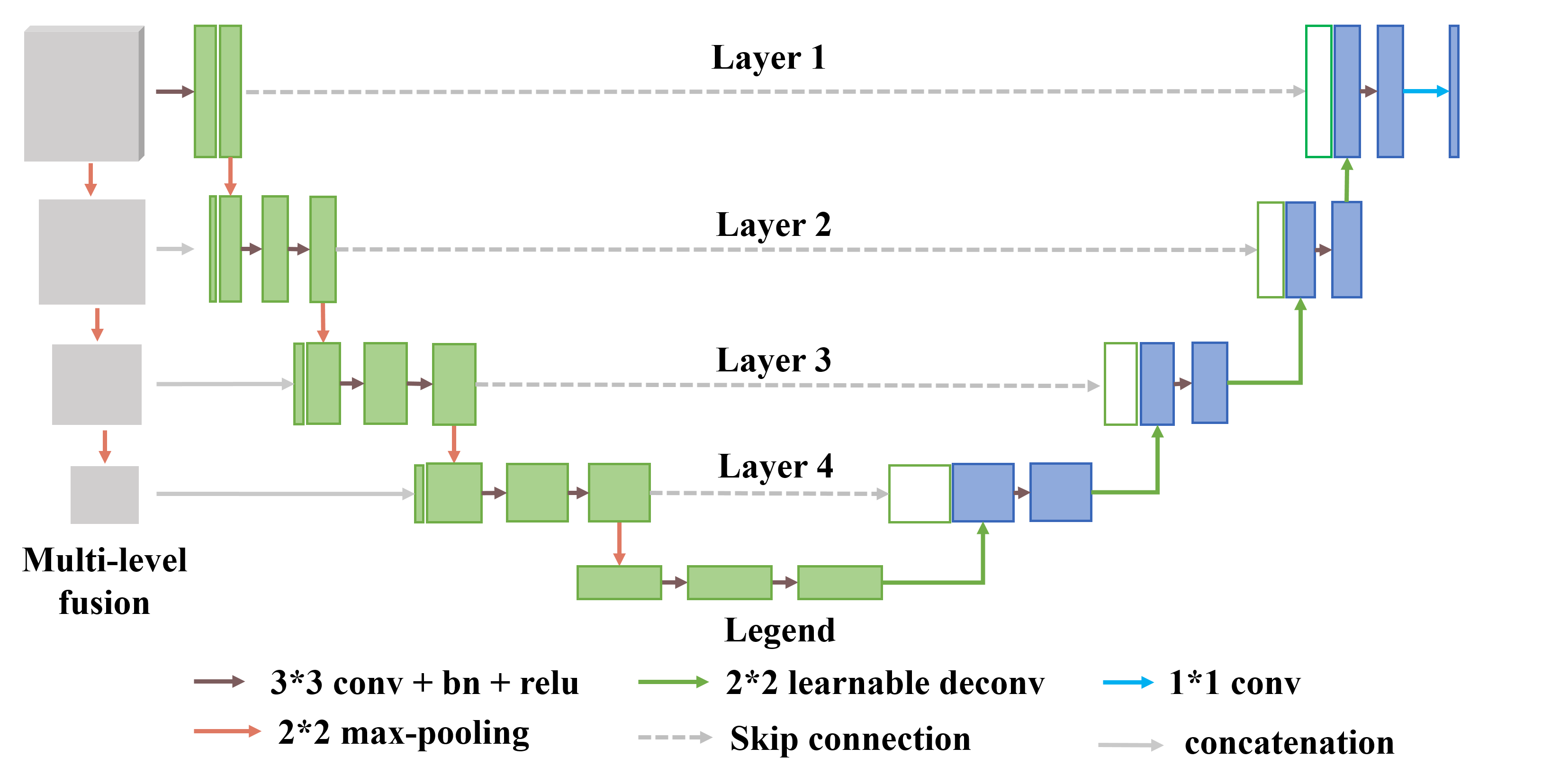
To improve the effect of model, we present a multi-level fusion strategy to make better use of multiple levels of information. As U-Net is a cascaded framework, with the number of convolution layers increases, it gradually extracts high-dimensional information representations. In layer 1 (as shown in Figure 3), U-Net may only learn simple boundary information, but in layer 4, it may be able to learn high-dimensional structural information, which is important in boundary detection on the polycrystalline image. The upper information sent to the network contains not only boundary information, but also rich structural information. Thus, we use a multi-level fusion strategy to make the most of it. The simplest concatenation is used as the fusion strategy.

Grain Object Tracking Slice By Slice

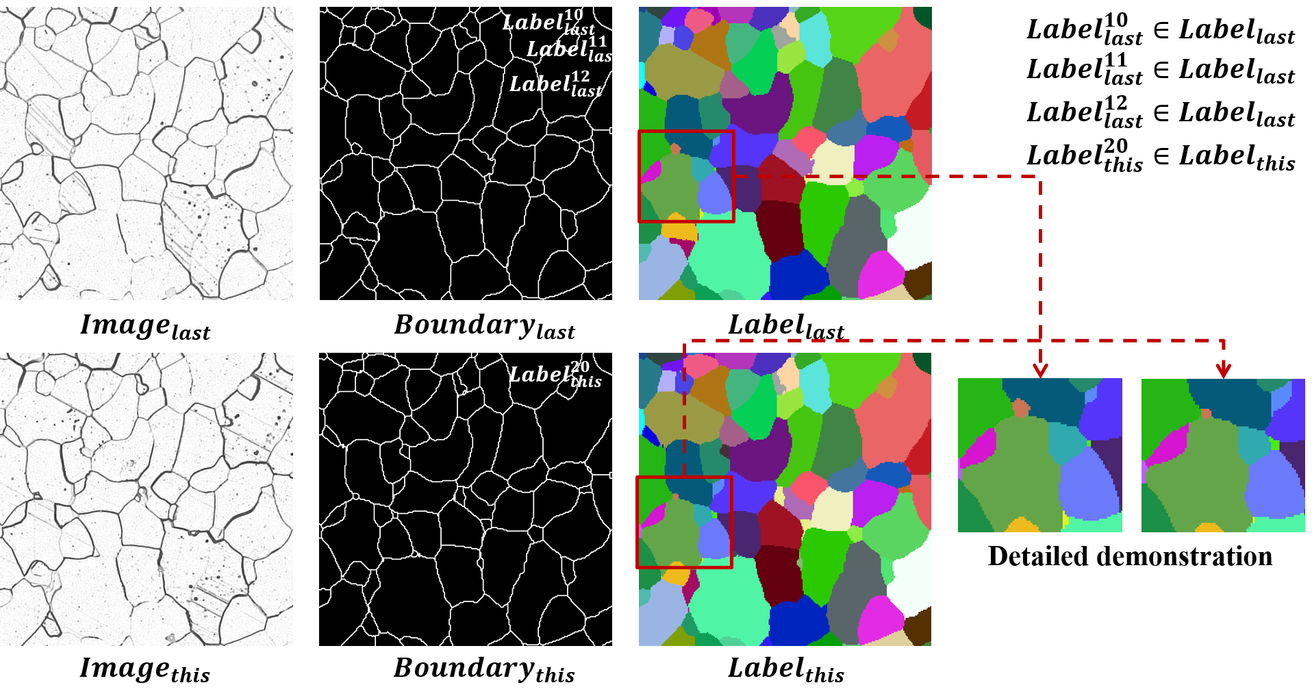
After analyzing all 2D images, there is still a task to reconstruct the 3D structure, which is to recognize the same grain regions in adjacent slices. As shown in Figure 4, Image_last and Image_this are two adjacent slices. Boundary_last and Boundary_this are boundary detection results. Label_last and Label_this are the label results, which can be used to 3D reconstruction. Each grain region is given to a unique label and a certain color to visualize. In Figure 4, various deformations such as deformation, appearance, disappearance may occur with grains in Z direction as shown in detailed demonstration. Therefore, there is a challenge to design an algorithm to solve all these deformations when transform boundary results to label result.

Figure 4: Tracking demonstration. The left column is raw images. The medium column is the boundary result. We need to track each grain between two neighbor slices and transform boundary to label. In label result, each grain region is given to a unique label and a certain color to visualize.

Traditional methods can not solve this problem very well, because they often produce over-segment results. Therefore, we intend to use a learning algorithm to handle this task. Unfortunately, many object tracking algorithms based on deep learning rely on the different appearance of each objects, which is very suited to track the objects in natural scene. By contrast, all the grains have the same pixel value in boundary result or approximate value in origin image.

We propose a new grain object tracking solution using convolution network in image classification task. For each pair of two connected grain regions in three dimensions, we apply a classification network to recognize whether they are belong to the same label.

Figure 5: we use image classification network to achieve the similarity of two regions. The similarity is the probability of success tracking.

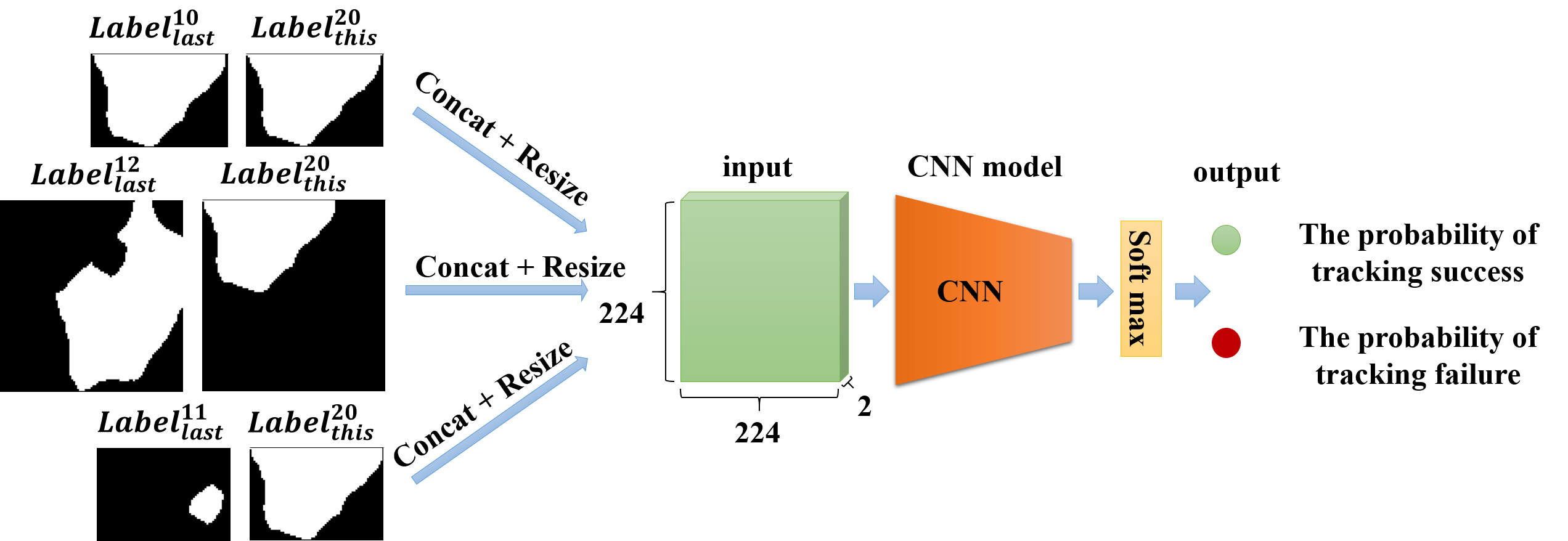
We use Figure 4 and Figure 5 for detailed illustration. Label_last is a set of labels in the last slice, and Label_this is a set of labels in this slice. We pick up image classification algorithm to track grain objects. For each grain in this slice, Label${}_{this}^{20}$ for example, we find its all connected components (such as Label${}_{last}^{10}$, Label${}_{last}^{11}$ and Label${}_{last}^{12}$) in Label_last in Z direction. Then we resize and concatenate each Label${}_{last}^{j}$ with Label${}_{this}^{20}$ to form 2 channels image and feed it to an image classification network. The network has simple 2-class output to get the similarity of two regions or the probability of successful tracking. After that, we can obtain the label $j$ of Label${}_{last}^{j}$ which has maximum similarity with Label${}_{this}^{20}$. If the maximum similarity is beyond a threshold, the tracking process can be thought to success and the label $j$ can be assigned to Label${}_{this}^{20}$.

The pure iron grain dataset

Recently progress in image segmentation has been driven by high-capacity models trained on large dataset. However, unlike public data in nature and biological scenes, the production and labeling of material microscopic image are very time-consuming. Because of the opacity of materials, scientist can only use serial section method to obtain the 2D slices (images) of materials. Besides, the images may suffer many flaws during sample preparation, which makes the labeling process consume much more time than other image data. In total, we think the progress of material microscopic image processing is hindered by the lack of public data.

Therefore, we present our dataset with its label in order to provide a referenced dataset for computer vision community. We provide two types of pure iron data, one real anisotropic dataset and one simulated isotropic dataset. The real dataset is produced and collected in practical experiments with serial section method. It has a stack of 296 microscopic pure iron slices with large resolution ($1024\times 1024$ pixels) for two classes (grain and grain boundary). The goal of processing task is to achieve 3D structure of microstructure. Usually, it is need to firstly detect single-pixel closed the boundary of each grain in each slice, and then reconstruct 3D information. The ground truth of real dataset is labeled by professional material researchers. The simulated dataset is generated by Monte Carlo Potts model, which is used to mimic grown procedure of polycrystalline grain. The simulated dataset consists of a sequence of 2D label slices and corresponding serial boundary images. It contains 400 slices with resolution of $400\times 400$ pixels. Due to the nature of simulation, it does not have the corresponding real original image. Besides, due to the polishing process of sample preparation, the resolution of Z direction is always smaller than X and Y direction for real dataset. By contrast, the simulated dataset is isotropic.

Experiment Results

In this section, adequate experiments will be deployed to demonstrate the effectiveness of our proposed method. We split the real dataset into a train set and a test set with 1:1 ratio, and take 32 continuous images from the train set as a validation set. To ensure sufficient training data, we perform random cropping, flipping and rotation of the data during the training process. And random seed is set for the repeatability of experiments. The test set and validation set use $256\times 256$ pixels images as the input of network and the results are gathered to form a $1024\times 1024$ slice by using overlap-tile strategy (?).

The goal of boundary detection in this work is to achieve single-pixel closed boundary of each grain. Thus, the metric should tolerate minor differences in boundary location between prediction and mask and pay attention to under-segment and over-segment errors.

For fair comparison, we use multiple metrics to evaluate our algorithm, such as Variation of Information (VI) (?; ?), Adjusted Rand Index (ARI) (?) and Mean Average Precision (mAP) (?; ?). For VI metric, a lower value indicates a better performance. While for the other metrics, a larger value indicates a better performance.

We first perform normalization to input images. The weights of nets are initialized with Xavier (?) and all nets are trained from scratch. We adapt batch normalization (BN) (?) after each convolution and before activation. All hidden layers are equipped with Rectified Linear Unit (ReLU (?)). The learning rate is set to 1e-4 initially, decaying by 80 percent per 10 epochs until 1e-6. We optimize the objective function with respect to the weights at all network layer by RMSProp with smoothing constant ($\alpha$)=0.9 and $\epsilon$=1e-5. Each model is trained for 500 epochs on 1 NVIDIA V100 GPU with a batch size of 24. Our implementation of this algorithm is derived from the publicly available Pytorch framework (?). During training, we pick up the parameters when it achieves the smallest loss on the validation set. All the performance in the experimental section Boundary Detection is obtained on the testing set using the above parameters. Except for some complex models, which we have reduced the batch size.

Algorithm	Loss		Mode		VI	mAP	ARI
	CBW	ABW	Layer 1	Layer 1-4
U-net	$\checkmark$	$\times$	$\times$	$\times$	0.3165	0.6067	0.8155
	$\times$	$\checkmark$	$\times$	$\times$	0.2952	0.6171	0.8297
Attention      U-net	$\checkmark$	$\times$	$\times$	$\times$	0.2828	0.6264	0.8298
	$\times$	$\checkmark$	$\times$	$\times$	0.2808	0.6298	0.8370
WPU-net	$\checkmark$	$\times$	$\checkmark$	$\times$	0.1868	0.6703	0.8530
	$\checkmark$	$\times$	$\times$	$\checkmark$	0.1894	0.6718	0.8516
	$\times$	$\checkmark$	$\checkmark$	$\times$	0.1929	0.6925	0.8634
	$\times$	$\checkmark$	$\times$	$\checkmark$	0.1874	0.6959	0.8647

Table 1: Ablation experiments results on loss and mode. CBW means the class-balanced weight, ABW means the adaptive boundary weight. The bold values mean the best performance in each metric.

Boundary Detection

All reported performance is the average of scores for all images in test set. To justify the effectiveness of our proposed adaptive weighted loss and WPU-Net, we have conducted a sufficient ablation experiment, the results are shown in Table 1 and 2. The following is detailed analysis and explanation of the experimental results.

Adaptive Boundary Weighting

As shown in Table 1, adaptive boundary weight (ABW) performs better than class-balanced weighted (CBW) loss in general, especially on mAP. We can see the VI score of CBW and ABW may behave differently on WPU-Net with Layer 1 mode, however, the mAP and ARI score of ABW always perform well. This may benefit from the excellent performance of ABW on small grains. As VI is less sensitive in tiny grains. We can also see that Adaptive Boundary Weight can achieve higher performance both on U-net and Attention U-net architecture. That is suggesting that improvements induced by adaptive boundary weight can be used directly with existing state-of-the-art architectures.

Integrate Propagative Information in Network

To systematically examine the effect of WPU-Net, we firstly conduct the experiment about two fusion modes. One mode is Layer 1, which means the last slice’s information is only merged in the first layer, another is Layer 1-4, means the multi-level strategy. We can see from Table 1 that the results with multi-level fusion are generally better, it proves the effectiveness of multi-level strategy. what should be noted is that in order to obtain a single-pixel boundary result image, all the predictions of networks will undergo skeletonization operation.

Another experiment we conduct is a model comparison between WPU-net and seven state-of-the-art methods, which are 3D U-Net (?), Attention U-Net (?), RDN (?), U-Net (?), UNet+BDCLSTM (?), HED (?) and Fast-FineCut (?). It should be mentioned that all the algorithms we used in this experiment are re-implemented using pytorch based on the original paper and source code (If it provides).

Algorithm	VI	MAP	ARI
WPU-net	0.1874	0.6959	0.8647
3D U-Net	0.2537	0.6496	0.8397
RDN	0.2691	0.6340	0.8418
Attention U-Net	0.2828	0.6264	0.8298
UNet+BDCLSTM	0.3134	0.6193	0.8135
U-Net	0.3165	0.6067	0.8155
Fast-FineCut	0.4183	0.5660	0.8030
HED	0.4436	0.5651	0.7635

Table 2: Model comparison in real dataset. The bold values mean the best performance in each metric.

Figure 6: Detection results with different methods. Four adjacent slices from top to bottom. The yellow arrows represent blurred or missing boundary that does not recover accurately. The blue arrows refer to scratches that does not eliminate. And the red circles mean break of boundary.

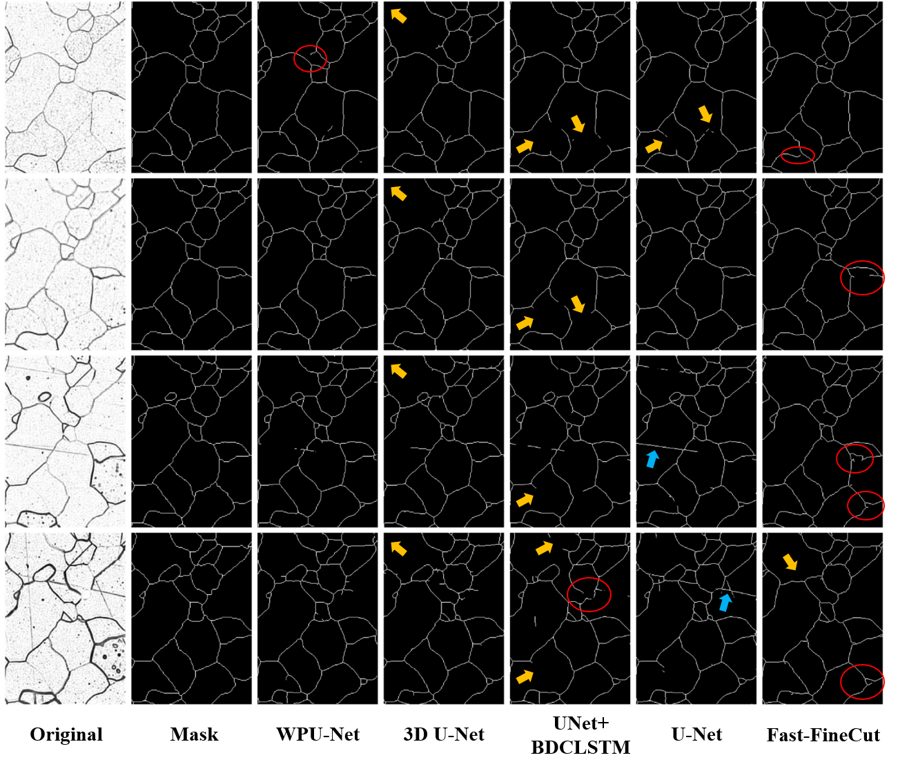
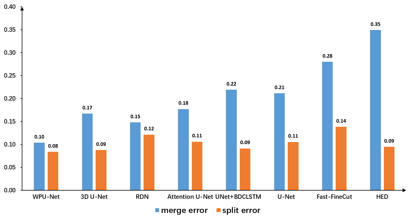
As shown in Table 2 and Figure 6, our proposed method WPU-net outperforms others in every evaluation metrics, especially on VI metrics (the summation of split error and merge error), our method is about $7\%$ smaller than other methods. This proves the feasibility and effectiveness of propagation segmentation network in the boundary detection task of 3D images, especially in polycrystalline materials. The problem of continuous blurring of same grain boundaries and scratch noise in adjacent slices are the two main reasons for the in-applicability of typical methods. To further analyze it, we display the merge error and split error of each method in VI evaluation metric separately in Figure 7. The merge error(under-segmentation) means the error caused by unsuccessful detection of grain boundaries(FN), resulting in two grains in the image being judged to be the same grain (usually occurs at blurred grain boundaries). While the split error (over-segmentation) means the wrong detection of grain boundaries(FP), resulting in one grain in the image is judged as two grains (usually occurs at spurious scratches). From Figure 7, we can see that other models all show much worse performance on blurred grain boundaries generally, except our method. However WPU-net performs better in both problems, especially on blurred boundaries. One interesting phenomenon is that the merge error is abnormally high in UNet+BDCLSTM when compared with the split error, it may indicate that RNN is not good at dealing with the problem of continuous missing.

Figure 7: Model comparison on merge error and split error.

Grain Object Tracking Slice By Slice

We evaluate our object tracking algorithm both on simulated isotropic dataset and real anisotropic dataset. We use VI and ARI as metrics of the object tracking experiments. We compare our algorithm with maximum overlap area algorithm and minimum centroid distance algorithm proposed in the article (?). For image classification model, we choose vgg13_bn (?) and densenet161 (?) for comparison. The learning rate started from 1e-4 and is multiplied by 0.8 after each epoch until decay to 1e-6. The batch size is 40 and uses RMSProp with 0.9 momentum to optimized. Each model was trained for 20 epochs. The tracking threshold is 0.5. The testing set was evaluated on the parameters where models achieve the highest accuracy on the validation set.

In addition, because of lacking information in Z dimension, the tracking algorithm can not achieve 100% accuracy even for ground truth boundary result. Therefore, we choose the best model tested with ground truth boundary tracking task and apply it to the boundary results with different boundary detecting methods. It is reasonable to use tracking results to evaluate the performance of different boundary detect methods.

Note that the number of images is not limitation for CNN classification. There are thousands of pair grain regions in two adjacent slices. Thus, there are million of pair grain regions as training set for real dataset and half million of pair grain regions as training set for simulated one.

Simulated Dataset

For simulated dataset, we use 240 slices as the training set, 80 slices as the validation set and 80 slices as the testing set. As shown in the Table.3, we report the tracking performance of different methods. Tracking methods with deep learning achieve the promising performance in comparison with traditional methods. Besides, it improves the performance when complex and advanced network is applied. However, the duration of deep learning based tracking algorithm consumes much more time than traditional methods. We think it can be optimized by parallel programming.

Algorithm	VI	ARI	Duration(s)
Min Centroid Dis	0.5798	0.9160	41.87
Max Overlap Area	0.5754	0.9206	42.97
Vgg13_bn	0.5832	0.9192	426.92
Densenet161	0.5124	0.9391	759.90

Table 3: Performance of tracking on simulated dataset with different algorithms.

Algorithm	VI	ARI	Duration(s)
Min Centroid Dis	0.5508	0.8856	1100.95
Max Overlap Area	0.6331	0.8582	1126.41
Vgg13_bn	0.5299	0.8972	7934.64
Densenet161	0.4829	0.9131	9228.82

Table 4: Performance of tracking on real dataset with different algorithms.

Algorithm	VI	ARI
WPU-Net	1.4785	0.7577
Fast-Fine Cut	1.7517	0.7050
3D U-net	1.4864	0.7405
Attention U-net	1.6701	0.7348
U-net	1.7326	0.6932
Unet-BDCLSTM	1.7363	0.6841

Table 5: Performance of tracking on real data set with different boundary detection algorithms.

Real Dataset

For real dataset, We use 116 slices as the training set, 32 slices as the validation set and 148 slices as the testing set. As shown in Table 4, it has shown the same result with simulated data. In addition, we choose the densenet161 to track the boundary result of different methods in Table 5. WPU-net achieves the promising result than other methods.

Conclusion

In this work, we propose a Weighted Propagation U-net (WPU-net) to handle the boundary detection in polycrystalline materials. The network integrates information from adjacent slices to aid boundary detection in target slice. And we present adaptive boundary weighting to optimize the model, which can tolerate minor difference in boundary detection and protect the topology of grains. Experiments have shown that our network achieves the promising performance that is superior to previous state-of-the-art methods. The VI metric (summation of merge and split error) of our method is about 7% smaller than the second-best method. In addition, we develop a new solution to reconstruct the 3D structure of the sample by using CNN to perform grain object tracking between slices. Our team will focus on accelerating the speed of tracking and optimizing boundary detection in the future.

References

- [Alom et al. 2018] Alom, M. Z.; Hasan, M.; Yakopcic, C.; Taha, T. M.; and Asari, V. K. 2018. Recurrent residual convolutional neural network based on u-net (r2u-net) for medical image segmentation. CoRR abs/1802.06955.
- [Cantwell et al. 2014] Cantwell, P. R.; Tang, M.; Dillon, S. J.; Luo, J.; Rohrer, G. S.; and Harmer, M. P. 2014. Grain boundary complexions. Acta Materialia 62(1):1–48.
- [Chen et al. 2016] Chen, J.; Yang, L.; Zhang, Y.; Alber, M. S.; and Chen, D. Z. 2016. Combining fully convolutional and recurrent neural networks for 3d biomedical image segmentation. neural information processing systems 3036–3044.
- [Cicek et al. 2016] Cicek, O.; Abdulkadir, A.; Lienkamp, S. S.; Brox, T.; and Ronneberger, O. 2016. 3d u-net: Learning dense volumetric segmentation from sparse annotation. medical image computing and computer assisted intervention 424–432.
- [Glorot and Bengio 2010] Glorot, X., and Bengio, Y. 2010. Understanding the difficulty of training deep feedforward neural networks. Proceedings of the thirteenth international conference on artificial intelligence and statistics 249–256.
- [Hamilton 2018] Hamilton, B. A. 2018. 2018 data science bowl. https://www.kaggle.com/c/data-science-bowl-2018/overview/evaluation.
- [Hu et al. 2017] Hu, J.; Shi, Y.; Sauvage, X.; Sha, G.; and Lu, K. 2017. Grain boundary stability governs hardening and softening in extremely fine nanograined metals. Science 355(6331):1292–1296.
- [Huang et al. 2017] Huang, G.; Liu, Z.; Der Maaten, L. V.; and Weinberger, K. Q. 2017. Densely connected convolutional networks. computer vision and pattern recognition 2261–2269.
- [Ioffe and Szegedy 2015] Ioffe, S., and Szegedy, C. 2015. Batch normalization: Accelerating deep network training by reducing internal covariate shift. international conference on machine learning 448–456.
- [Januszewski et al. 2018] Januszewski, M.; Kornfeld, J.; Li, P. H.; Pope, A.; Blakely, T.; Lindsey, L.; Maitinshepard, J.; Tyka, M.; Denk, W.; and Jain, V. 2018. High-precision automated reconstruction of neurons with flood-filling networks. Nature Methods 15(8):605–610.
- [Krizhevsky, Sutskever, and Hinton 2012] Krizhevsky, A.; Sutskever, I.; and Hinton, G. E. 2012. Imagenet classification with deep convolutional neural networks. neural information processing systems 141(5):1097–1105.
- [Lee et al. 2017] Lee, K.; Zung, J.; Li, P. H.; Jain, V.; and Seung, H. S. 2017. Superhuman accuracy on the snemi3d connectomics challenge. arXiv: Computer Vision and Pattern Recognition.
- [Lin et al. 2014] Lin, T.; Maire, M.; Belongie, S. J.; Hays, J.; Perona, P.; Ramanan, D.; Dollar, P.; and Zitnick, C. L. 2014. Microsoft coco: Common objects in context. In European conference on computer vision, 740–755.
- [Long, Shelhamer, and Darrell 2015] Long, J.; Shelhamer, E.; and Darrell, T. 2015. Fully convolutional networks for semantic segmentation. computer vision and pattern recognition 3431–3440.
- [Ma et al. 2018] Ma, B.; Ban, X.; Huang, H.; Chen, Y.; Liu, W.; and Zhi, Y. 2018. Deep learning-based image segmentation for al-la alloy microscopic images. Symmetry 10(4):107.
- [Ma et al. 2019] Ma, B.; Ban, X.; Su, Y.; Liu, C.; Wang, H.; Xue, W.; Zhi, Y.; and Wu, D. 2019. Fast-finecut: Grain boundary detection in microscopic images considering 3d information. Micron 116:5–14.
- [Meilă 2007] Meilă, M. 2007. Comparing clusterings—an information based distance. Journal of Multivariate Analysis 98(5):873–895.
- [Meyer 1992] Meyer, F. 1992. Color image segmentation. International Conference on Image Processing and its Applications 303–306.
- [Milletari, Navab, and Ahmadi 2016] Milletari, F.; Navab, N.; and Ahmadi, S. 2016. V-net: Fully convolutional neural networks for volumetric medical image segmentation. international conference on 3d vision 565–571.
- [Nuneziglesias et al. 2013] Nuneziglesias, J.; Kennedy, R.; Parag, T.; Shi, J.; and Chklovskii, D. B. 2013. Machine learning of hierarchical clustering to segment 2d and 3d images. PLOS ONE 8(8).
- [Oktay et al. 2018] Oktay, O.; Schlemper, J.; Folgoc, L. L.; Lee, M.; Heinrich, M.; Misawa, K.; Mori, K.; Mcdonagh, S.; Hammerla, N. Y.; and Kainz, B. 2018. Attention u-net: Learning where to look for the pancreas. In International Conference on Medical Imaging with Deep Learning.
- [Pytorch 2019] Pytorch. 2019. https://pytorch.org/.
- [Ronneberger, Fischer, and Brox 2015] Ronneberger, O.; Fischer, P.; and Brox, T. 2015. U-net: Convolutional networks for biomedical image segmentation. medical image computing and computer assisted intervention 234–241.
- [Simonyan and Zisserman 2015] Simonyan, K., and Zisserman, A. 2015. Very deep convolutional networks for large-scale image recognition. international conference on learning representations.
- [Vinh, Epps, and Bailey 2010] Vinh, N. X.; Epps, J.; and Bailey, J. 2010. Information theoretic measures for clusterings comparison: Variants, properties, normalization and correction for chance. Journal of Machine Learning Research 11:2837–2854.
- [Waggoner et al. 2013] Waggoner, J. W.; Zhou, Y.; Simmons, J. P.; De Graef, M.; and Wang, S. 2013. 3d materials image segmentation by 2d propagation: A graph-cut approach considering homomorphism. IEEE Transactions on Image Processing 22(12):5282–5293.
- [Xie and Tu 2015] Xie, S., and Tu, Z. 2015. Holistically-nested edge detection. international conference on computer vision 1395–1403.
- [Xue 2016] Xue, W. 2016. Three-dimensional Modeling and Quantitative Characterization of Grain Structure. Ph.D. Dissertation, University of Science and Technology Beijing.
- [Zeng 2016] Zeng, T. 2016. Residual deconvolutional networks for brain electron microscopy image segmentation. IEEE Transactions on Medical Imaging.