Regulation of renewable resource exploitation

Idris Kharroubi111Sorbonne Université, LPSM, idris.kharroubi @upmc.fr.    Thomas Lim222Laboratoire d’Analyse et Probabilités, Université d’Evry-Val d’Essonne and ENSIIE, lim@ensiie.fr.    Thibaut Mastrolia333CMAP, Ecole Polytechnique, IP Paris, thibaut.mastrolia@polytechnique.edu. This author acknowledges the financial supports of the Chaire Financial Risks hosted by the Louis Bachelier Institute and the ANR project PACMAN ANR-16-CE05-0027.
Abstract

We investigate the impact of a regulation policy imposed on an agent exploiting a possibly renewable natural resource. We adopt a principal-agent model in which the Principal looks for a contract, i.e.formulae-sequence𝑖𝑒i.e. taxes/compensations, leading the Agent to a certain level of exploitation. For a given contract, we first describe the Agent’s optimal harvest using the BSDE theory. Under regularity and boundedness assumptions on the coefficients, we express almost optimal contracts as solutions to HJB equations. We then extend the result to coefficients with less regularity and logistic dynamics for the natural resource. We end by numerical examples to illustrate the impact of the regulation in our model.

Key words: Contract Theory, BSDEs, HJB PDE, Logistic SDE.

1 Introduction

The exploitation of natural resources is fundamental for the survival and development of the growing human population. However, natural resources are limited since they are either non renewable (e.g. minerals, oil, gas and coal) so that the available quantity is limited, or renewable (e.g. food, water and forests) and in this case the natural resource is limited by its ability to renew itself. In particular, an excessive exploitation of such resources might lead to their extinctions and therefore affect the depending economies with, for instance, high increases of prices and higher uncertainty on the future. Thus, the natural resource manager faces a dilemma: either harvesting intensively the resource to increase her incomes, or taking into account the potential externalities induced by an overexploitation of the resource and impacting her future ability to harvest the resource. It has been nevertheless emphasized in [7] that in some cases it is optimal for natural resource manager to harvest until the extinction of the resource. This optimal harvesting strategy thus leads to costs for the global welfare related to the environment degradation.

Therefore, the management and the monitoring of the exploitation of natural resources are a balance between optimal harvest for the natural resource manager and ecological implications for public organizations. This second issue has attracted a lot of interest, especially from governance institutions. For example in its last annual report on sustainable development, the statistical office of the European Union Eurostat dedicates a full section to the question of sustainable consumption and production (see [11], Section 12).

The management of natural resources have also attracted a lot of interest from the academic community. Many studies on natural resources exploitation tried to describe the possible effect of economic incentives on the exploitation (see e.g. [5, 14, 26, 15]). These references stress the need of an incentive policy to ensure the sustainability of the resource. However, even if the regulator have access to the abundance level of natural resource, the unobservability of the natural resource manager behavior induces moral hazards. Thus, the regulator’s issue is to incentivize the resource manager to optimally reduce the cost of the resource degradation, together with ensuring a minimal incomes for the manager, under moral hazard. To the best of our knowledge, this question has been addressed only in the discrete-time framework (see for instance [13]) without considering any randomness in the dynamics of the resource. The aim of this work is to investigate this problem in continuous time with randomness in the system.

To deal with this issue, we consider a principal-agent model under moral hazard. The first elements of contract theory with moral hazard appeared in the 60’s with the articles [3, 29] in which the mechanisms of controlled management were investigated. Then, it has been extended and named as agency problem (see among others [28, 23]) by considering discrete-time models. Concerning the continuous-time framework, the agency problem with moral hazard has been first studied in [16] by modelling the uncertainty of risky incomes with a Brownian motion.

The agency problem can be roughly described as follows. We associate a moral hazard problem with a Stackelberg game in which the leader (named the Principal) proposes at time 00 a compensation to the follower (named the Agent) given at a maturity T>0𝑇0T>0 fixed by the contract, to manage the wealth of the leader. Moreover, the Principal has to propose a compensation high enough (called the reservation utility) to ensure a certain level of utility for the Agent. Although the Principal cannot directly observe the action of the Agent, the former can anticipate the best reaction effort of the latter with respect to a fixed compensation. Hence the agency problem remains to design an optimal compensation proposed by the Principal to the Agent given all the constraints mentioned above under moral hazard.

The common approach to solve this problem consists in proceeding in two steps. The first step is to compute the optimal reaction of the Agent given a fixed compensation proposed by the Principal, i.e. solving the utility maximization problem of the Agent. In all the papers mentioned above, the shape of considered contracts is fundamental to solve the Agent problem by assuming that the compensation is composed by

  • a constant part depending on the reservation utility of the Agent,

  • a part indexed by the (risky) incomes of the Principal,

  • the certain equivalent gain of utility appearing in the Agent maximization.

Using the theory of Backward Stochastic Differential Equations (BSDE for short), [9] proved that this class of smooth contracts, having a relevant economic interpretation, is not restrictive to solve the agency problem. The second step consists in solving the Principal problem. Taking into account this optimal reaction of the Agent, the goal is to compute the optimal compensation. As emphasized in [25] and then in [8, 9], this problem remains to a (classical) stochastic control problem with the wealth of the Principal and the continuation utility value of the Agent as state variables.

In this paper, we identify the natural resource manager as the Agent. The Principal refers to a regulator, which can be a public institution that monitors the resource manager’s activities.

The resource manager can either harvest or renew the natural resource. In the first case the production is sold at a given price on the market and in the second case the resource manager pays for each unit of renewed natural resource. To regulate the natural resource exploitation, the Principal imposes a tax/compensation to the Agent depending on the remaining level of resource at the terminal time horizon. We suppose here that the Agent is risk-averse and we model his preference with an exponential utility function444See for instance [4] for more details on this kind of utility function and the economical interpretations of it.. For a given harvesting strategy, the Agent total gain is composed by the cumulated amounts paid/earned by renewing/harvesting the natural resource and the regulation compensation/tax. The Agent’s aim is then to maximize the expected utility of his total gain over possible harvesting strategies.

On the other side, given the previous optimal harvest of the Agent, the regulator aims at fixing a tax/compensation policy that incentives the Agent to let a reasonable remaining level of natural resource. As a public institution, we assume that the regulator is risk-neutral.

The main features to model the dynamic of a renewable natural resource are its birth and death rates and the inter-species competition. Besides, due to random evolution of the population, we consider uncertainty in the available abundance. Following [12, 2, 21] we choose to model the evolution of the natural resource by a stochastic logistic diffusion.

We then focus on the Principal-agent problem. We first characterize the Agent behavior for a fixed regulation policy represented by a random variable ξ𝜉\xi. Following the BSDEs approaches to deal with exponential utility maximization, we get a unique optimal harvesting strategy as a function of the Z𝑍Z component of the solution to a quadratic BSDE with terminal condition ξ𝜉\xi (see [24, 17]).

We next turn to the regulator problem which consists in maximizing an expected terminal reward depending on the regulation tax ξ𝜉\xi and the level of remaining natural resource according to the Agent’s optimal response. By writing the explicit form of the resource manager’s optimal strategy, we turn the regulator problem into a Markov stochastic control problem of a diffusion with controlled drift. We then look for a regular solution to the related PDE to proceed by verification. However, in our case we face the following three issues.

  • By considering the logistic dynamics for the resource abundance population, the HJB PDE related to the Principal problem involves a term of the form x2xvsuperscript𝑥2subscript𝑥𝑣x^{2}\partial_{x}v where x𝑥x stands for the resource population abundance and v𝑣v is the Principal’s value function. This term, induced by the inter-species competition in the classical logistic case, prevents us from using existence results of regular solutions to PDEs.

  • The shape of the optimal harvest of the manager leads to irregular coefficients for the related PDE, which also prevents from getting regular solutions.

  • Due to the exponential preferences of the Agent, the Principal’s admissible strategies need to satisfy an exponential integrability condition. However, the linear preferences of the Principal leads to an optimal contract that is not necessarily exponential integrable. Therefore, the regulator problem might not have an optimal regulation policy.

To deal with these issues, we first study a model for which the inter-species competition coefficient μ𝜇\mu of the population is bounded. Hence, the term x2xvsuperscript𝑥2subscript𝑥𝑣x^{2}\partial_{x}v is replaced by xμ(x)xv𝑥𝜇𝑥subscript𝑥𝑣x\mu(x)\partial_{x}v. We then construct a regular approximation of the Hamiltonian. By considering the related PDE, we derive a regular solution (see Proposition 4.1) together with an almost optimal control satisfying the admissibility condition (see Theorem 4.2). We notice that our approach can be related to that of Fleming and Soner [27], which consists in an approximating the value function by a sequence of smooth value functions to derive a dynamic programming principle. We next turn to the logistic case i.e.formulae-sequence𝑖𝑒i.e. μ(x)=x𝜇𝑥𝑥\mu(x)=x for which we show that the almost optimal strategy obtained for a truncation of μ𝜇\mu remains an almost optimal strategy for a large value of the truncation parameter (see Theorem 4.3).

We finally illustrate our results by numerical experiments. We compute the almost optimal strategies using approximations of solutions to HJB PDEs and show that the regulation has a significant effect on the level of remaining natural resource.

The remainder of the paper is the following. In Section 2 we describe the considered mathematical problem. We then solve in Section 3 the manager’s problem for a given regulation policy. In Section 4, we first provide almost optimal strategies in the case where the coefficient μ𝜇\mu is bounded and we extend our result to the logisitic dynamics. We end Section 4 by economical insights and numerical experiments.

Notations and spaces

We give in this part all the notations used in this paper. Let (Ω,,)Ω(\Omega,{\cal F},\mathbb{P}) be a complete probability space. We assume that this space is equipped with a standard Brownian motion W𝑊W and we denote by 𝔽:=(t)t0assign𝔽subscriptsubscript𝑡𝑡0\mathbb{F}:=({\cal F}_{t})_{t\geq 0} its right-continuous and complete natural filtration.

Let p1𝑝1p\geq 1 and a time horizon T>0𝑇0T>0, we introduce the following spaces

  • 𝒫()𝒫\mathcal{P}(\mathbb{R}) (resp. 𝒫r()𝒫𝑟\mathcal{P}r(\mathbb{R})) will denote the σ𝜎\sigma-algebra of \mathbb{R}-progressively mesurable, 𝔽𝔽\mathbb{F}-adapted (resp. 𝔽𝔽\mathbb{F}-predictable) integrable processes.

  • 𝒮Tpsubscriptsuperscript𝒮𝑝𝑇\mathcal{S}^{p}_{T} is the set of processes X,𝒫()𝑋𝒫X,\,\mathcal{P}(\mathbb{R})-mesurable and continuous satisfying

    𝔼[sup0tT|Xt|p]<+.𝔼delimited-[]subscriptsupremum0𝑡𝑇superscriptsubscript𝑋𝑡𝑝\mathbb{E}[\sup_{0\leq t\leq T}|X_{t}|^{p}]<+\infty\;.
  • Tpsubscriptsuperscript𝑝𝑇\mathbb{H}^{p}_{T} is the set of processes X,𝒫r()𝑋𝒫𝑟X,\,\mathcal{P}r(\mathbb{R})-mesurable satisfying

    𝔼[(0T|Xt|2𝑑t)p2]<+.𝔼delimited-[]superscriptsuperscriptsubscript0𝑇superscriptsubscript𝑋𝑡2differential-d𝑡𝑝2\mathbb{E}\Big{[}\big{(}\int_{0}^{T}|X_{t}|^{2}dt\big{)}^{\frac{p}{2}}\Big{]}<+\infty\;.
  • For an integer q0𝑞0q\geq 0, a subset D𝐷D of qsuperscript𝑞\mathbb{R}^{q} and for any ν(0,1)𝜈01\nu\in(0,1), we denote by C1+ν(D)superscript𝐶1𝜈𝐷C^{1+\nu}(D) the set of continuously differentiable functions f:D:𝑓𝐷f:~{}D\rightarrow\mathbb{R} such that

    |f|1=supxD(|f(x)|+1iq|xif(x)|+supx,yD1iq|xif(x)xif(y)||xy|ν)<,subscript𝑓1subscriptsupremum𝑥𝐷𝑓𝑥subscript1𝑖𝑞subscriptsubscript𝑥𝑖𝑓𝑥subscriptsupremum𝑥𝑦𝐷subscript1𝑖𝑞subscriptsubscript𝑥𝑖𝑓𝑥subscriptsubscript𝑥𝑖𝑓𝑦superscript𝑥𝑦𝜈|f|_{1}=\sup_{x\in D}\Big{(}|f(x)|+\sum_{1\leq i\leq q}|\partial_{x_{i}}f(x)|+\sup_{x,y\in D}\sum_{1\leq i\leq q}\frac{|\partial_{x_{i}}f(x)-\partial_{x_{i}}f(y)|}{|x-y|^{\nu}}\Big{)}<\infty\;,

    and by C2+ν(D)superscript𝐶2𝜈𝐷C^{2+\nu}(D) the set of twice continuously differentiable functions f:D:𝑓𝐷f:~{}D\rightarrow\mathbb{R} such that

    |f|2+νsubscript𝑓2𝜈\displaystyle|f|_{2+\nu} =\displaystyle= supxD(|f(x)|+1iq|xif(x)|+1i,jq|xi,xjf(x)|)subscriptsupremum𝑥𝐷𝑓𝑥subscript1𝑖𝑞subscriptsubscript𝑥𝑖𝑓𝑥subscriptformulae-sequence1𝑖𝑗𝑞subscriptsubscript𝑥𝑖subscript𝑥𝑗𝑓𝑥\displaystyle\sup_{x\in D}\Big{(}|f(x)|+\sum_{1\leq i\leq q}|\partial_{x_{i}}f(x)|+\sum_{1\leq i,j\leq q}|\partial_{x_{i},x_{j}}f(x)|\Big{)}
    +supx,yD1i,jq|xi,xjf(x)xi,xjf(y)||xy|ν<.subscriptsupremum𝑥𝑦𝐷subscriptformulae-sequence1𝑖𝑗𝑞subscriptsubscript𝑥𝑖subscript𝑥𝑗𝑓𝑥subscriptsubscript𝑥𝑖subscript𝑥𝑗𝑓𝑦superscript𝑥𝑦𝜈\displaystyle+\sup_{x,y\in D}\sum_{1\leq i,j\leq q}\frac{|\partial_{x_{i},x_{j}}f(x)-\partial_{x_{i},x_{j}}f(y)|}{|x-y|^{\nu}}~{}<~{}\infty\;.

2 The model

2.1 The natural resource

We fix a deterministic time horizon T>0𝑇0T>0 and we suppose that the natural resource abundance Xtμsuperscriptsubscript𝑋𝑡𝜇X_{t}^{\mu} at time t0𝑡0t\geq 0 is given by

Xtμ=X0+0tXsμ(λμ(Xsμ))𝑑s+0tσXsμ𝑑Ws,t[0,T],formulae-sequencesuperscriptsubscript𝑋𝑡𝜇subscript𝑋0superscriptsubscript0𝑡superscriptsubscript𝑋𝑠𝜇𝜆𝜇superscriptsubscript𝑋𝑠𝜇differential-d𝑠superscriptsubscript0𝑡𝜎superscriptsubscript𝑋𝑠𝜇differential-dsubscript𝑊𝑠𝑡0𝑇X_{t}^{\mu}=X_{0}+\int_{0}^{t}X_{s}^{\mu}(\lambda-\mu(X_{s}^{\mu}))ds+\int_{0}^{t}\sigma X_{s}^{\mu}dW_{s}\;,\quad t\in[0,T]\;, (2.1)

where X0subscript𝑋0X_{0}, λ𝜆\lambda and σ𝜎\sigma are positive constants. The quantities X0subscript𝑋0X_{0} and λ𝜆\lambda correspond to the initial natural resource abundance and the growth rate respectively. The map μ𝜇\mu represents the competition inside the species considered or more generally an auto-degradation parameter for a natural resource. We assume that the map μ𝜇\mu satisfies the following assumption

(H0) μ𝜇\mu is a map from +subscript\mathbb{R}_{+} to +subscript\mathbb{R}_{+} such that (2.1) admits a unique strong solution in 𝒮T2subscriptsuperscript𝒮2𝑇\mathcal{S}^{2}_{T}.

Note that Assumption (H0) holds for instance if the map xxμ(x)𝑥𝑥𝜇𝑥x\longmapsto x\mu(x) is Lipschitz continuous. Another important example is the so-called logistic equation where μ(x)=x𝜇𝑥𝑥\mu(x)=x on +subscript\mathbb{R}_{+}, see for example in [12]. In this last case, SDE (2.1) admits an explicit unique solution that will be denoted in the sequel by X𝑋X and given by

Xt=X0e(λσ22)t+σWt1+X00te(λσ22)s+σWs𝑑s,t[0,T].formulae-sequencesubscript𝑋𝑡subscript𝑋0superscript𝑒𝜆superscript𝜎22𝑡𝜎subscript𝑊𝑡1subscript𝑋0superscriptsubscript0𝑡superscript𝑒𝜆superscript𝜎22𝑠𝜎subscript𝑊𝑠differential-d𝑠𝑡0𝑇X_{t}=\frac{X_{0}e^{(\lambda-\frac{\sigma^{2}}{2})t+\sigma W_{t}}}{1+X_{0}\int_{0}^{t}e^{(\lambda-\frac{\sigma^{2}}{2})s+\sigma W_{s}}ds}\;,\quad t\in[0,T]\;.

The ecological interpretation of this model is the following. At time t𝑡t, if the coefficient μ(Xtμ)𝜇superscriptsubscript𝑋𝑡𝜇\mu(X_{t}^{\mu}) is larger than λ𝜆\lambda then the drift of the diffusion is negative. Therefore the abundance of the natural resource Xtμsuperscriptsubscript𝑋𝑡𝜇X_{t}^{\mu} decreases in mean. Conversely, if μ(Xtμ)𝜇superscriptsubscript𝑋𝑡𝜇\mu(X_{t}^{\mu}) is smaller than λ𝜆\lambda then the drift of the diffusion is positive. Hence, the abundance Xtμsuperscriptsubscript𝑋𝑡𝜇X_{t}^{\mu} increases in mean. For more details see for instance [21, Proposition 3.4].

More general models can be used in practice and one of the main challenges, see [21], is to rely branching processes with birth and death intensities to the solutions of continuous SDEs.

2.2 The Agent’s problem

We consider an agent who tries to make profit from the natural resource. We suppose that this agent owns facilities to either harvest or renew this resource. We assume that his action happends continuously in time and we denote by αtsubscript𝛼𝑡\alpha_{t} his intervention rate at time t𝑡t, i.e. the abundance Xtμsuperscriptsubscript𝑋𝑡𝜇X_{t}^{\mu} will decrease of an amount αtXtμsubscript𝛼𝑡superscriptsubscript𝑋𝑡𝜇\alpha_{t}X_{t}^{\mu} per unit of time. This means that if the intervention rate αtsubscript𝛼𝑡\alpha_{t} is positive (resp. negative), the Agent harvests (resp. renews) the natural resource. We denote by 𝒜𝒜\mathcal{A} the set of 𝔽𝔽\mathbb{F}-adapted processes defined on [0,T]0𝑇[0,T] and valued in [M¯,M¯]¯𝑀¯𝑀[-\underline{M},\overline{M}] where M¯¯𝑀\underline{M} and M¯¯𝑀\overline{M} are two nonnegative constants. If the Agent is prohibited to renew the resource then M¯=0¯𝑀0\underline{M}=0. This set 𝒜𝒜{\cal A} is called the set of admissible actions.

To take into account the control α𝛼\alpha of the Agent on the natural resource abundance, we introduce the probability measure αsuperscript𝛼\mathbb{P}^{\alpha} defined by its density Hαsuperscript𝐻𝛼H^{\alpha} w.r.t. \mathbb{P} given by

dαd|T:=HTα,assignevaluated-at𝑑superscript𝛼𝑑subscript𝑇subscriptsuperscript𝐻𝛼𝑇{d\mathbb{P}^{\alpha}\over d\mathbb{P}}\Big{|}_{{\cal F}_{T}}:=H^{\alpha}_{T}\;,

where the process Hαsuperscript𝐻𝛼H^{\alpha} is defined by

Htα:=exp(0tαsσ𝑑Ws120s|αsσ|2𝑑s),t[0,T].formulae-sequenceassignsubscriptsuperscript𝐻𝛼𝑡superscriptsubscript0𝑡subscript𝛼𝑠𝜎differential-dsubscript𝑊𝑠12superscriptsubscript0𝑠superscriptsubscript𝛼𝑠𝜎2differential-d𝑠𝑡0𝑇H^{\alpha}_{t}:=\exp\Big{(}-\int_{0}^{t}{\alpha_{s}\over\sigma}dW_{s}-{1\over 2}\int_{0}^{s}\Big{|}{\alpha_{s}\over\sigma}\Big{|}^{2}ds\Big{)}\;,\quad t\in[0,T]\;.

In the sequel, we denote by 𝔼αsuperscript𝔼𝛼\mathbb{E}^{\alpha} and 𝔼tαsubscriptsuperscript𝔼𝛼𝑡\mathbb{E}^{\alpha}_{t} the expectation and conditional expectation given tsubscript𝑡{\cal F}_{t} respectively, for any t[0,T]𝑡0𝑇t\in[0,T], under the probability measure αsuperscript𝛼\mathbb{P}^{\alpha}.

For α𝒜𝛼𝒜\alpha\in{\cal A}, we get from Girsanov Theorem (see e.g. Theorem 5.1 in [18]) that the process Wαsuperscript𝑊𝛼W^{\alpha} defined by

Wtα:=Wt+0tαsσ𝑑s,t[0,T],formulae-sequenceassignsuperscriptsubscript𝑊𝑡𝛼subscript𝑊𝑡superscriptsubscript0𝑡subscript𝛼𝑠𝜎differential-d𝑠𝑡0𝑇W_{t}^{\alpha}:=W_{t}+\int_{0}^{t}\frac{\alpha_{s}}{\sigma}ds\;,\quad t\in[0,T]\;,

is a Brownian motion under the probability αsuperscript𝛼\mathbb{P}^{\alpha}. Thus, for a given admissible effort α𝒜𝛼𝒜\alpha\in{\cal A}, the dynamics of X𝑋X can be rewritten under the probability αsuperscript𝛼\mathbb{P}^{\alpha} as

Xtμ=x+0t(Xsμ(λμ(Xsμ))αsXsμ)𝑑s+0tσXsμ𝑑Wsα,t[0,T].formulae-sequencesuperscriptsubscript𝑋𝑡𝜇𝑥superscriptsubscript0𝑡superscriptsubscript𝑋𝑠𝜇𝜆𝜇superscriptsubscript𝑋𝑠𝜇subscript𝛼𝑠superscriptsubscript𝑋𝑠𝜇differential-d𝑠superscriptsubscript0𝑡𝜎superscriptsubscript𝑋𝑠𝜇differential-dsubscriptsuperscript𝑊𝛼𝑠𝑡0𝑇X_{t}^{\mu}=x+\int_{0}^{t}\big{(}X_{s}^{\mu}(\lambda-\mu(X_{s}^{\mu}))-\alpha_{s}X_{s}^{\mu}\big{)}ds+\int_{0}^{t}\sigma X_{s}^{\mu}dW^{\alpha}_{s}\;,\quad t\in[0,T]\;.

This new dynamics reflects the evolution of the population with a rate αtsubscript𝛼𝑡\alpha_{t} per unit of time. Hence, αtXtμsubscript𝛼𝑡superscriptsubscript𝑋𝑡𝜇\alpha_{t}X_{t}^{\mu} has to be seen as the speed of the exploitation of the natural resource at time t𝑡t.

We then are given a price function p:++:𝑝subscriptsubscriptp:~{}\mathbb{R}_{+}\rightarrow\mathbb{R}_{+} and we suppose that the price per unit of the natural resource on the market is given by p(Xtμ)𝑝superscriptsubscript𝑋𝑡𝜇p(X_{t}^{\mu}) at time t0𝑡0t\geq 0. We make the following assumption on the price function p𝑝p.

(Hp) There exists a constant P𝑃P such that p(x)xP𝑝𝑥𝑥𝑃p(x)x\leq P for all x[0,+)𝑥0x\in[0,+\infty).

This price function p𝑝p allows to take into account the dependence w.r.t. the abundance (the more abundant the resource is, the cheaper it will be and conversely). Such a price dependence has already been used to model liquidity effects on financial market, where empirical studies showed that the impact is of the form p(x)=Peβ1xβ2𝑝𝑥𝑃superscript𝑒subscript𝛽1superscript𝑥subscript𝛽2p(x)=Pe^{-\beta_{1}x^{\beta_{2}}}, x+𝑥subscriptx\in\mathbb{R}_{+}, for some positive constants P𝑃P, β1subscript𝛽1\beta_{1} and β2subscript𝛽2\beta_{2} (see e.g. [1, 20]). In particular, (Hp) is satisfied for this type of dependence. Another basic example for which (Hp) holds is the case p(x)=Px1𝑝𝑥𝑃superscript𝑥1p(x)=Px^{-1}, x>0𝑥0x>0. This last example reflects the inability to buy the natural resource once it is extinct.

We assume that the manager sells the harvested resource on the market at price p(Xtμ)𝑝superscriptsubscript𝑋𝑡𝜇p(X_{t}^{\mu}) per unit at time t𝑡t if αtsubscript𝛼𝑡\alpha_{t} is positive, and pays the price p(Xtμ)𝑝superscriptsubscript𝑋𝑡𝜇p(X_{t}^{\mu}) per unit of natural resource at time t𝑡t if αtsubscript𝛼𝑡\alpha_{t} is negative to renew this one. This provides the global amount 0Tp(Xtμ)Xtμαt𝑑tsuperscriptsubscript0𝑇𝑝subscriptsuperscript𝑋𝜇𝑡subscriptsuperscript𝑋𝜇𝑡subscript𝛼𝑡differential-d𝑡\int_{0}^{T}p(X^{\mu}_{t})X^{\mu}_{t}\alpha_{t}dt over the time horizon [0,T]0𝑇[0,T].

We also suppose that giving an effort is costly for the manager and we consider the classical quadratic cost function k:+:𝑘subscriptk:\mathbb{R}\rightarrow\mathbb{R}_{+} given by k(α)=|α|22,αformulae-sequence𝑘𝛼superscript𝛼22𝛼k(\alpha)=\frac{|\alpha|^{2}}{2},\;\alpha\in\mathbb{R}. Thus, the Agent is penalized by the instantaneous amount k(αt)𝑘subscript𝛼𝑡k(\alpha_{t}) per unit of time for a given effort α𝒜𝛼𝒜\alpha\in{\cal A}. This leads to the global payment 0Tk(αt)𝑑tsuperscriptsubscript0𝑇𝑘subscript𝛼𝑡differential-d𝑡\int_{0}^{T}k(\alpha_{t})dt over the considered time horizon [0,T]0𝑇[0,T].

In our investigation, we recall that the activity of the natural resource manager is regulated by an institution (usually an environment administration) who is taking care about the size of the remaining natural resource. To avoid an over-exploitation, the regulator imposes a tax on the Agent depending on the remaining resource. This tax amount is represented by an Tsubscript𝑇{\cal F}_{T}-measurable random variable ξ𝜉\xi and is paid at time T𝑇T. Note that ξ𝜉\xi can be either positive or negative. In this last case, it means that the regulator gives a compensation to the manager.

Throughout the paper we assume that the Agent’s preferences are given by the exponential utility function uAsubscript𝑢𝐴u_{A} defined by

uA(x):=exp(γx),x,formulae-sequenceassignsubscript𝑢𝐴𝑥𝛾𝑥𝑥u_{A}(x):=-\exp\big{(}-\gamma x\big{)}\;,\quad x\in\mathbb{R}\;,

where γ𝛾\gamma is a positive constant corresponding to the risk aversion of the Agent. We define the value function VA(ξ)subscript𝑉𝐴𝜉V_{A}(\xi) of the Agent associated to the taxation policy ξ𝜉\xi by

VA(ξ):=supα𝒜𝔼α[exp(γ(0Tp(Xsμ)Xsμαs𝑑s0T|αs|22𝑑sξ))].assignsubscript𝑉𝐴𝜉subscriptsupremum𝛼𝒜superscript𝔼𝛼delimited-[]𝛾superscriptsubscript0𝑇𝑝superscriptsubscript𝑋𝑠𝜇subscriptsuperscript𝑋𝜇𝑠subscript𝛼𝑠differential-d𝑠superscriptsubscript0𝑇superscriptsubscript𝛼𝑠22differential-d𝑠𝜉V_{A}(\xi):=\sup_{\alpha\in{\cal A}}\mathbb{E}^{\alpha}\Big{[}-\exp\Big{(}-\gamma\big{(}\int_{0}^{T}p(X_{s}^{\mu})X^{\mu}_{s}\alpha_{s}ds-\int_{0}^{T}\frac{|\alpha_{s}|^{2}}{2}ds-\xi\big{)}\Big{)}\Big{]}\;. (2.2)

For a fixed tax ξ𝜉\xi, we denote by 𝒜(ξ)superscript𝒜𝜉\mathcal{A}^{*}(\xi) the set of efforts α𝒜superscript𝛼𝒜\alpha^{*}\in{\cal A} satisfying the following equality

𝔼α[exp(γ(0Tp(Xsμ)Xsμαs𝑑s0T|αs|22𝑑sξ))]=VA(ξ).superscript𝔼superscript𝛼delimited-[]𝛾superscriptsubscript0𝑇𝑝superscriptsubscript𝑋𝑠𝜇superscriptsubscript𝑋𝑠𝜇subscriptsuperscript𝛼𝑠differential-d𝑠superscriptsubscript0𝑇superscriptsubscriptsuperscript𝛼𝑠22differential-d𝑠𝜉subscript𝑉𝐴𝜉\mathbb{E}^{{\alpha^{*}}}\Big{[}-\exp\Big{(}-\gamma\big{(}\int_{0}^{T}p(X_{s}^{\mu})X_{s}^{\mu}\alpha^{*}_{s}ds-\int_{0}^{T}\frac{|\alpha^{*}_{s}|^{2}}{2}ds-\xi\big{)}\Big{)}\Big{]}=V_{A}(\xi)\;.

An effort α𝒜(ξ)superscript𝛼superscript𝒜𝜉\alpha^{*}\in{\cal A}^{*}(\xi) is said to be optimal for the fixed tax ξ𝜉\xi.

2.3 The Principal’s problem

The aim of the regulator is to stabilize the resource population at a fixed target size at the maturity T𝑇T. For that, a tax ξ𝜉\xi is chosen to incentivize the Agent to manage the natural resource so that the remaining population is close to the targeted size. Hence, the regulator benefits from the tax paid by the Agent and is penalized through a cost function f𝑓f depending on the size of the resource at maturity T𝑇T. The expected reward under the action α𝒜𝛼𝒜\alpha\in{\cal A} of the Agent is then given by

𝔼α[ξf(XTμ)].superscript𝔼𝛼delimited-[]𝜉𝑓superscriptsubscript𝑋𝑇𝜇\mathbb{E}^{{\alpha}}\big{[}\xi-f(X_{T}^{\mu})\big{]}\;.

Typically, we have in mind f(x)=c(βx)+𝑓𝑥𝑐superscript𝛽𝑥f(x)=c(\beta-x)^{+} meaning that the regulator targets a population size β>0𝛽0\beta>0 at time T𝑇T for the sustainability of the resource and pays the cost c𝑐c per unit if the natural resource is over-consumed. This function f𝑓f can be seen as the amount that the regulator must pay to reintroduce the missing resource.

We suppose that the resource manager is rational. Therefore, the Principal anticipates that for a tax ξ𝜉\xi, the Agent will choose an effort α𝛼\alpha in the set 𝒜(ξ)superscript𝒜𝜉\mathcal{A}^{*}(\xi). Note that this set is not necessarily reduced to a singleton555 In our investigation, we will show that the set 𝒜(ξ)superscript𝒜𝜉\mathcal{A}^{*}(\xi) is reduced to a single element., hence, as usual in moral hazard problems (see for instance [16] for the formulation of the moral hazard problem), the regulator solves

supξVP(ξ), with VP(ξ)=supα𝒜(ξ)𝔼α[ξf(XTμ)],subscriptsupremum𝜉superscript𝑉𝑃𝜉 with superscript𝑉𝑃𝜉subscriptsupremum𝛼superscript𝒜𝜉superscript𝔼𝛼delimited-[]𝜉𝑓superscriptsubscript𝑋𝑇𝜇\sup_{\xi}V^{P}(\xi)\;,\text{ with }V^{P}(\xi)=\sup_{\alpha\in\mathcal{A}^{*}(\xi)}\mathbb{E}^{{\alpha}}\Big{[}\xi-f(X_{T}^{\mu})\Big{]}, (2.3)

where ξ𝜉\xi lives in a set of suitable contracts defined in the following section.

2.4 Class of contracts and utility reservation

We now introduce a reserve utility R𝑅R which is a negative constant. This reserve means that the regulator cannot penalize too strongly the Agent for economical reasons so that the utility VA(ξ)subscript𝑉𝐴𝜉V_{A}(\xi) expected by the Agent has to be greater than R𝑅R. For instance, we can choose R𝑅R such that the regulator monitors the Agent by promising the same expected utility as the case without regulation (see Section 4.3.1 for more details). This example reflects a non-punitive taxation policy in which the regulator purely monitors the activities of the Agent. In our model, the sign of the tax ξ𝜉\xi is on purpose. This means that the natural resource manager pays the fee to the regulator when ξ𝜉\xi is positive and conversely, the regulator compensates the Agent’s activity when ξ𝜉\xi is negative. Moreover, we need to impose an exponential integrability on the tax ξ𝜉\xito ensure the well-posdness of VA(ξ)subscript𝑉𝐴𝜉V_{A}(\xi). We therefore introduce the class 𝒞Rμsubscriptsuperscript𝒞𝜇𝑅{\cal C}^{\mu}_{R} of admissible taxes defined as the set of Tsubscript𝑇\mathcal{F}_{T}-measurable random variables ξ𝜉\xi such that

VA(ξ)R,subscript𝑉𝐴𝜉𝑅V_{A}(\xi)\geq R\;, (2.4)

and there exists a constant γ>2γsuperscript𝛾2𝛾\gamma^{\prime}>2\gamma such that

𝔼[exp(γ|ξ|)]<+.𝔼delimited-[]superscript𝛾𝜉\mathbb{E}\big{[}\exp(\gamma^{\prime}|\xi|)\big{]}<+\infty\;. (2.5)

This last condition is very convenient since it allows to deal with the problem by using the theory of BSDEs. Moreover, a straightforward application of Cauchy-Schwarz inequality ensures that the optimization problems VA(ξ)subscript𝑉𝐴𝜉V_{A}(\xi) and VP(ξ)superscript𝑉𝑃𝜉V^{P}(\xi) take finite values.

3 Optimal effort of the natural resource’s manager

We first solve the optimal problem of the Agent (2.2) under taxation policy ξ𝒞Rμ𝜉superscriptsubscript𝒞𝑅𝜇\xi\in{\cal C}_{R}^{\mu}. As in [9], the following result shows that solving the Agent problem gives both an optimal effort αsuperscript𝛼\alpha^{*} and a particular representation of the tax ξ𝜉\xi with respect to the solution of a BSDE.

Theorem 3.1.

Let ξ𝒞Rμ𝜉subscriptsuperscript𝒞𝜇𝑅\xi\in\mathcal{C}^{\mu}_{R} and Assumption (Hp) be satisfied. There exists a unique pair (Y0,Z)(,R~]×T2subscript𝑌0𝑍~𝑅subscriptsuperscript2𝑇(Y_{0},Z)\in(-\infty,\tilde{R}]\times\mathbb{H}^{2}_{T} with R~:=log(R)γassign~𝑅𝑅𝛾\tilde{R}:=\frac{\log(-R)}{\gamma} such that

  1. (i)

    the tax has the following decomposition

    ξ=Y00T(g(Xtμ,Zt)+σ22γ|Zt|2)𝑑t+0TσZt𝑑Wt,𝜉subscript𝑌0superscriptsubscript0𝑇𝑔superscriptsubscript𝑋𝑡𝜇subscript𝑍𝑡superscript𝜎22𝛾superscriptsubscript𝑍𝑡2differential-d𝑡superscriptsubscript0𝑇𝜎subscript𝑍𝑡differential-dsubscript𝑊𝑡\xi=Y_{0}-\int_{0}^{T}\big{(}g(X_{t}^{\mu},Z_{t})+\frac{\sigma^{2}}{2}\gamma|Z_{t}|^{2}\big{)}dt+\int_{0}^{T}\sigma Z_{t}dW_{t}\;, (3.6)

    where g𝑔g is defined for any (x,z)+×𝑥𝑧subscript(x,z)\in\mathbb{R}_{+}\times\mathbb{R} by

    g(x,z)=|a(x,z)|22p(x)xa(x,z)a(x,z)z,𝑔𝑥𝑧superscriptsuperscript𝑎𝑥𝑧22𝑝𝑥𝑥superscript𝑎𝑥𝑧superscript𝑎𝑥𝑧𝑧g(x,z)=\frac{|a^{*}(x,z)|^{2}}{2}-p(x)xa^{*}(x,z)-a^{*}(x,z)z\;,

    and

    a(x,z)=((p(x)x+z)(M¯))M¯,superscript𝑎𝑥𝑧𝑝𝑥𝑥𝑧¯𝑀¯𝑀a^{*}(x,z)=\big{(}(p(x)x+z)\vee(-\underline{M})\big{)}\wedge\overline{M}\;, (3.7)
  2. (ii)

    the value of the Agent is given by

    VA(ξ)=exp(γY0),subscript𝑉𝐴𝜉𝛾subscript𝑌0V_{A}(\xi)=-\exp(\gamma Y_{0})\;,
  3. (iii)

    the process α(ξ)superscript𝛼𝜉\alpha^{*}(\xi) defined by αt(ξ)=a(Xtμ,Zt)subscriptsuperscript𝛼𝑡𝜉superscript𝑎superscriptsubscript𝑋𝑡𝜇subscript𝑍𝑡\alpha^{*}_{t}(\xi)=a^{*}(X_{t}^{\mu},Z_{t}) is the unique optimal effort associated with the tax ξ𝜉\xi given by (3.6).

Proof.

The proof is divided in three steps and is related to the BSDE associated with the value function of the Agent. We first introduce a dynamic extension of the optimization problem (2.2). We denote by J(t,ξ)𝐽𝑡𝜉J(t,\xi) the dynamic value function of the Agent at time t𝑡t for a tax ξ𝜉\xi which is defined by

J(t,ξ):=essinfα𝒜𝔼tα[exp(γ(tTp(Xsμ)Xsμαs𝑑stTk(αs)𝑑sξ))].assign𝐽𝑡𝜉subscriptessinf𝛼𝒜subscriptsuperscript𝔼𝛼𝑡delimited-[]𝛾superscriptsubscript𝑡𝑇𝑝superscriptsubscript𝑋𝑠𝜇superscriptsubscript𝑋𝑠𝜇subscript𝛼𝑠differential-d𝑠superscriptsubscript𝑡𝑇𝑘subscript𝛼𝑠differential-d𝑠𝜉J(t,\xi):=\mathop{\mathrm{ess\;inf}}_{\alpha\in{\cal A}}\mathbb{E}^{\alpha}_{t}\Big{[}\exp\Big{(}-\gamma\big{(}\int_{t}^{T}p(X_{s}^{\mu})X_{s}^{\mu}\alpha_{s}ds-\int_{t}^{T}k(\alpha_{s})ds-\xi\big{)}\Big{)}\Big{]}\;.

Note that VA(ξ)=J(0,ξ)subscript𝑉𝐴𝜉𝐽0𝜉V_{A}(\xi)=-J(0,\xi).

Step 1. Dynamic utility of the Agent and BSDE. We characterize J(,ξ)𝐽𝜉J(\cdot,\xi) as the unique solution of a BSDE and we derive the optimal control by using comparison results.

Let α𝒜𝛼𝒜\alpha\in{\cal A}, we introduce the process Jα(ξ)superscript𝐽𝛼𝜉J^{\alpha}(\xi) defined by

Jtα(ξ):=𝔼tα[exp(γ(tTp(Xsμ)Xsμαs𝑑stTk(αs)𝑑sξ))],assignsubscriptsuperscript𝐽𝛼𝑡𝜉superscriptsubscript𝔼𝑡superscript𝛼delimited-[]𝛾superscriptsubscript𝑡𝑇𝑝superscriptsubscript𝑋𝑠𝜇superscriptsubscript𝑋𝑠𝜇subscript𝛼𝑠differential-d𝑠superscriptsubscript𝑡𝑇𝑘subscript𝛼𝑠differential-d𝑠𝜉J^{\alpha}_{t}(\xi):=\mathbb{E}_{t}^{\mathbb{P}^{\alpha}}\Big{[}\exp\Big{(}-\gamma\big{(}\int_{t}^{T}p(X_{s}^{\mu})X_{s}^{\mu}\alpha_{s}ds-\int_{t}^{T}k(\alpha_{s})ds-\xi\big{)}\Big{)}\Big{]}\;,

so that

J(t,ξ):=essinfα𝒜tJtα(ξ).assign𝐽𝑡𝜉subscriptessinf𝛼subscript𝒜𝑡subscriptsuperscript𝐽𝛼𝑡𝜉J(t,\xi):=\mathop{\mathrm{ess\;inf}}_{\alpha\in{\cal A}_{t}}J^{\alpha}_{t}(\xi)\;. (3.8)

Step 1a. Martingale representation and integrability.

We know that the process Htα(exp(γ0t(k(αs)p(Xsμ)Xsμαs)𝑑s)Jtα(ξ))0tTsuperscriptsubscript𝐻𝑡𝛼subscript𝛾superscriptsubscript0𝑡𝑘subscript𝛼𝑠𝑝superscriptsubscript𝑋𝑠𝜇superscriptsubscript𝑋𝑠𝜇subscript𝛼𝑠differential-d𝑠subscriptsuperscript𝐽𝛼𝑡𝜉0𝑡𝑇H_{t}^{\alpha}(\exp(\gamma\int_{0}^{t}\big{(}k(\alpha_{s})-p(X_{s}^{\mu})X_{s}^{\mu}\alpha_{s}\big{)}ds)J^{\alpha}_{t}(\xi))_{0\leq t\leq T} is a (,𝔽)𝔽(\mathbb{P},\mathbb{F})-martingale. In view of the condition (2.5), there exists ε>0𝜀0\varepsilon>0 and q>1𝑞1q>1 such that (2+ε)qγγ2𝜀𝑞𝛾superscript𝛾(2+\varepsilon)q\gamma\leq\gamma^{\prime}. Hence, for p>1𝑝1p>1 such that 1p+1q=11𝑝1𝑞1\frac{1}{p}+\frac{1}{q}=1, since α𝛼\alpha is bounded and Condition (2.5) is satisfied, we get from Hölder’s inequality

𝔼[|H¯TαJTα(ξ)|2+ε]𝔼delimited-[]superscriptsuperscriptsubscript¯𝐻𝑇𝛼superscriptsubscript𝐽𝑇𝛼𝜉2𝜀\displaystyle\mathbb{E}[|\overline{H}_{T}^{\alpha}J_{T}^{\alpha}(\xi)|^{2+\varepsilon}] \displaystyle\leq 𝔼[|H¯Tα|(2+ε)p]1p𝔼[|e(2+ε)qγξ|]1q<+,𝔼superscriptdelimited-[]superscriptsuperscriptsubscript¯𝐻𝑇𝛼2𝜀𝑝1𝑝𝔼superscriptdelimited-[]superscript𝑒2𝜀𝑞𝛾𝜉1𝑞\displaystyle\mathbb{E}[|\overline{H}_{T}^{\alpha}|^{(2+\varepsilon)p}]^{\frac{1}{p}}\mathbb{E}[|e^{(2+\varepsilon)q\gamma\xi}|]^{\frac{1}{q}}~{}<~{}+\infty\;,

where H¯tα:=Htαexp(γ0t(k(αs)p(Xsμ)Xsμαs)𝑑s)assignsuperscriptsubscript¯𝐻𝑡𝛼superscriptsubscript𝐻𝑡𝛼𝛾superscriptsubscript0𝑡𝑘subscript𝛼𝑠𝑝superscriptsubscript𝑋𝑠𝜇superscriptsubscript𝑋𝑠𝜇subscript𝛼𝑠differential-d𝑠\overline{H}_{t}^{\alpha}:=H_{t}^{\alpha}\exp\Big{(}\gamma\int_{0}^{t}\big{(}k(\alpha_{s})-p(X_{s}^{\mu})X_{s}^{\mu}\alpha_{s}\big{)}ds\Big{)}. Hence, by using Doob’s maximal inequality, H¯αJα(ξ)𝒮2+εsuperscript¯𝐻𝛼superscript𝐽𝛼𝜉superscript𝒮2𝜀\overline{H}^{\alpha}J^{\alpha}(\xi)\in\mathcal{S}^{2+\varepsilon}. So by using the martingale representation theorem, we know there exists a process Z¯αT2+εsuperscript¯𝑍𝛼subscriptsuperscript2𝜀𝑇\overline{Z}^{\alpha}\in\mathbb{H}^{2+\varepsilon}_{T} such that

H¯tαJtα(ξ)superscriptsubscript¯𝐻𝑡𝛼subscriptsuperscript𝐽𝛼𝑡𝜉\displaystyle{\overline{H}}_{t}^{\alpha}J^{\alpha}_{t}(\xi) =\displaystyle= J0α+0tσZ¯sα𝑑Ws,t[0,T].subscriptsuperscript𝐽𝛼0superscriptsubscript0𝑡𝜎subscriptsuperscript¯𝑍𝛼𝑠differential-dsubscript𝑊𝑠𝑡0𝑇\displaystyle J^{\alpha}_{0}+\int_{0}^{t}\sigma\overline{Z}^{\alpha}_{s}dW_{s}\;,\quad t\in[0,T]\;.

Therefore, Jαsuperscript𝐽𝛼J^{\alpha} satisfies

dJtα(ξ)𝑑subscriptsuperscript𝐽𝛼𝑡𝜉\displaystyle dJ^{\alpha}_{t}(\xi) =\displaystyle= (αtZ~tαγ(k(αt)p(Xtμ)Xtμαt)Jtα(ξ))dt+σZ~tαdWt,subscript𝛼𝑡subscriptsuperscript~𝑍𝛼𝑡𝛾𝑘subscript𝛼𝑡𝑝superscriptsubscript𝑋𝑡𝜇superscriptsubscript𝑋𝑡𝜇subscript𝛼𝑡subscriptsuperscript𝐽𝛼𝑡𝜉𝑑𝑡𝜎subscriptsuperscript~𝑍𝛼𝑡𝑑subscript𝑊𝑡\displaystyle(\alpha_{t}\tilde{Z}^{\alpha}_{t}-\gamma(k(\alpha_{t})-p(X_{t}^{\mu})X_{t}^{\mu}\alpha_{t})J^{\alpha}_{t}(\xi))dt+\sigma\tilde{Z}^{\alpha}_{t}dW_{t}\;,

where Z~tα=Z¯tαH¯tα+Jtααtσ2subscriptsuperscript~𝑍𝛼𝑡subscriptsuperscript¯𝑍𝛼𝑡superscriptsubscript¯𝐻𝑡𝛼superscriptsubscript𝐽𝑡𝛼subscript𝛼𝑡superscript𝜎2\tilde{Z}^{\alpha}_{t}=\frac{\overline{Z}^{\alpha}_{t}}{{\overline{H}}_{t}^{\alpha}}+J_{t}^{\alpha}\frac{\alpha_{t}}{\sigma^{2}} for any t[0,T]𝑡0𝑇t\in[0,T], and JTα(ξ)=exp(γξ)superscriptsubscript𝐽𝑇𝛼𝜉𝛾𝜉J_{T}^{\alpha}(\xi)=\exp(\gamma\xi).

We now prove that Z~αT2superscript~𝑍𝛼superscriptsubscript𝑇2\tilde{Z}^{\alpha}\in\mathbb{H}_{T}^{2}. From (2.5), the boundedness of α𝛼\alpha and Assumption (Hp), there exists a positive constant C>0𝐶0C>0 such that

𝔼[0T|Z¯tαH¯tα+Jtααtσ2|2𝑑t]𝔼delimited-[]superscriptsubscript0𝑇superscriptsubscriptsuperscript¯𝑍𝛼𝑡superscriptsubscript¯𝐻𝑡𝛼superscriptsubscript𝐽𝑡𝛼subscript𝛼𝑡superscript𝜎22differential-d𝑡\displaystyle\mathbb{E}\Big{[}\int_{0}^{T}|\frac{\overline{Z}^{\alpha}_{t}}{{\overline{H}}_{t}^{\alpha}}+J_{t}^{\alpha}\frac{\alpha_{t}}{\sigma^{2}}|^{2}dt\Big{]} \displaystyle\leq 2(𝔼[0T|Z¯tαH¯tα|2𝑑t]+𝔼[0T|Jtααtσ2|2𝑑t])2𝔼delimited-[]superscriptsubscript0𝑇superscriptsubscriptsuperscript¯𝑍𝛼𝑡superscriptsubscript¯𝐻𝑡𝛼2differential-d𝑡𝔼delimited-[]superscriptsubscript0𝑇superscriptsuperscriptsubscript𝐽𝑡𝛼subscript𝛼𝑡superscript𝜎22differential-d𝑡\displaystyle 2\Big{(}\mathbb{E}\Big{[}\int_{0}^{T}|\frac{\overline{Z}^{\alpha}_{t}}{{\overline{H}}_{t}^{\alpha}}|^{2}dt\Big{]}+\mathbb{E}\Big{[}\int_{0}^{T}|J_{t}^{\alpha}\frac{\alpha_{t}}{\sigma^{2}}|^{2}dt\Big{]}\Big{)}
\displaystyle\leq C(1+𝔼[0T|Z¯tαH¯tα|2𝑑t]).𝐶1𝔼delimited-[]superscriptsubscript0𝑇superscriptsubscriptsuperscript¯𝑍𝛼𝑡superscriptsubscript¯𝐻𝑡𝛼2differential-d𝑡\displaystyle C\Big{(}1+\mathbb{E}\Big{[}\int_{0}^{T}|\frac{\overline{Z}^{\alpha}_{t}}{{\overline{H}}_{t}^{\alpha}}|^{2}dt\Big{]}\Big{)}\;.

We set q~:=1+ε2assign~𝑞1𝜀2\tilde{q}:=1+\frac{\varepsilon}{2} and p~>1~𝑝1\tilde{p}>1 such that 1p~+1q~=11~𝑝1~𝑞1\frac{1}{\tilde{p}}+\frac{1}{\tilde{q}}=1. Using Hölder and BDG Inequalities and since Z¯αT2+εsuperscript¯𝑍𝛼subscriptsuperscript2𝜀𝑇\overline{Z}^{\alpha}\in\mathbb{H}^{2+\varepsilon}_{T}, we get

𝔼[0T|Z¯tαH¯tα|2𝑑t]𝔼delimited-[]superscriptsubscript0𝑇superscriptsubscriptsuperscript¯𝑍𝛼𝑡superscriptsubscript¯𝐻𝑡𝛼2differential-d𝑡\displaystyle\mathbb{E}[\int_{0}^{T}|\frac{\overline{Z}^{\alpha}_{t}}{{\overline{H}}_{t}^{\alpha}}|^{2}dt] \displaystyle\leq 𝔼[supt[0,T]|(H¯tα)1|20T|Z¯tα|2𝑑t]𝔼delimited-[]subscriptsupremum𝑡0𝑇superscriptsuperscriptsuperscriptsubscript¯𝐻𝑡𝛼12superscriptsubscript0𝑇superscriptsubscriptsuperscript¯𝑍𝛼𝑡2differential-d𝑡\displaystyle\mathbb{E}[\sup_{t\in[0,T]}|({\overline{H}}_{t}^{\alpha})^{-1}|^{2}\int_{0}^{T}|\overline{Z}^{\alpha}_{t}|^{2}dt]
\displaystyle\leq 𝔼[supt[0,T]|(H¯tα)1|2p~]1p~𝔼[(0T|Z¯tα|2𝑑t)q~]1q~𝔼superscriptdelimited-[]subscriptsupremum𝑡0𝑇superscriptsuperscriptsuperscriptsubscript¯𝐻𝑡𝛼12~𝑝1~𝑝𝔼superscriptdelimited-[]superscriptsuperscriptsubscript0𝑇superscriptsubscriptsuperscript¯𝑍𝛼𝑡2differential-d𝑡~𝑞1~𝑞\displaystyle\mathbb{E}[\sup_{t\in[0,T]}|({\overline{H}}_{t}^{\alpha})^{-1}|^{2\tilde{p}}]^{\frac{1}{\tilde{p}}}\mathbb{E}[\big{(}\int_{0}^{T}|\overline{Z}^{\alpha}_{t}|^{2}dt\big{)}^{\tilde{q}}]^{\frac{1}{\tilde{q}}}
<\displaystyle< +.\displaystyle+\infty\;.

Consequently, we get Z~αT2superscript~𝑍𝛼superscriptsubscript𝑇2\tilde{Z}^{\alpha}\in\mathbb{H}_{T}^{2}.

Step 1b. Comparison of BSDEs and optimal effort. We now turn to the characterization of the solution to (3.8) by a BSDE. We introduce the following BSDE

dJ¯t(ξ)𝑑subscript¯𝐽𝑡𝜉\displaystyle d\underline{J}_{t}(\xi) =\displaystyle= infa[M¯,M¯]G(Xtμ,J¯t(ξ),Z¯~t,a)dt+σZ¯~tdWt,J¯T(ξ)=exp(γξ),subscriptinfimum𝑎¯𝑀¯𝑀𝐺superscriptsubscript𝑋𝑡𝜇subscript¯𝐽𝑡𝜉subscript¯~𝑍𝑡𝑎𝑑𝑡𝜎subscript¯~𝑍𝑡𝑑subscript𝑊𝑡subscript¯𝐽𝑇𝜉𝛾𝜉\displaystyle-\inf_{a\in[-\underline{M},\overline{M}]}G(X_{t}^{\mu},\underline{J}_{t}(\xi),\underline{\tilde{Z}}_{t},a)dt+\sigma\underline{\tilde{Z}}_{t}dW_{t}\;,\quad\underline{J}_{T}(\xi)=\exp(\gamma\xi)\;, (3.9)

where

G(x,j,z~,a)𝐺𝑥𝑗~𝑧𝑎\displaystyle G(x,j,\tilde{z},a) :=assign\displaystyle:= γ(k(a)p(x)xa)jaz~.𝛾𝑘𝑎𝑝𝑥𝑥𝑎𝑗𝑎~𝑧\displaystyle\gamma(k(a)-p(x)xa)j-a\tilde{z}\;.

This BSDE has a Lipschitz generator and square integrable terminal condition from (2.5). Therefore it admits a unique solution in 𝒮2×T2superscript𝒮2superscriptsubscript𝑇2\mathcal{S}^{2}\times\mathbb{H}_{T}^{2}. Moreover, for any α𝒜𝛼𝒜\alpha\in\mathcal{A}, we notice that (Jα(ξ),Z~α)superscript𝐽𝛼𝜉superscript~𝑍𝛼(J^{\alpha}(\xi),\tilde{Z}^{\alpha}) satisfies the following BSDE

dJtα(ξ)𝑑subscriptsuperscript𝐽𝛼𝑡𝜉\displaystyle d{J}^{\alpha}_{t}(\xi) =\displaystyle= G(Xtμ,Jtα(ξ),Z~tα,αt)dt+σZ~tαdWt,JTα(ξ)=exp(γξ).𝐺superscriptsubscript𝑋𝑡𝜇subscriptsuperscript𝐽𝛼𝑡𝜉subscriptsuperscript~𝑍𝛼𝑡subscript𝛼𝑡𝑑𝑡𝜎subscriptsuperscript~𝑍𝛼𝑡𝑑subscript𝑊𝑡subscriptsuperscript𝐽𝛼𝑇𝜉𝛾𝜉\displaystyle-G(X_{t}^{\mu},{J}^{\alpha}_{t}(\xi),{\tilde{Z}}^{\alpha}_{t},\alpha_{t})dt+\sigma{\tilde{Z}}^{\alpha}_{t}dW_{t}\;,\quad{J}^{\alpha}_{T}(\xi)=\exp(\gamma\xi)\;.

By classical comparison Theorem, we have

J¯t(ξ)subscript¯𝐽𝑡𝜉\displaystyle\underline{J}_{t}(\xi) \displaystyle\leq J(t,ξ),t[0,T].𝐽𝑡𝜉for-all𝑡0𝑇\displaystyle J(t,\xi)\;,\quad\forall t\in[0,T]\;.

Then, we notice that BSDE (3.9) can be rewritten

dJ¯t(ξ)𝑑subscript¯𝐽𝑡𝜉\displaystyle d\underline{J}_{t}(\xi) =\displaystyle= G(Xtμ,J¯t(ξ),Z¯~t,a(Xtμ,Z¯~tγJ¯t(ξ)))dt+σZ¯~tdWt,J¯T(ξ)=exp(γξ).𝐺superscriptsubscript𝑋𝑡𝜇subscript¯𝐽𝑡𝜉subscript¯~𝑍𝑡superscript𝑎superscriptsubscript𝑋𝑡𝜇subscript¯~𝑍𝑡𝛾subscript¯𝐽𝑡𝜉𝑑𝑡𝜎subscript¯~𝑍𝑡𝑑subscript𝑊𝑡subscript¯𝐽𝑇𝜉𝛾𝜉\displaystyle-G\Big{(}X_{t}^{\mu},\underline{J}_{t}(\xi),\underline{\tilde{Z}}_{t},{a^{*}}\big{(}X_{t}^{\mu},\frac{\underline{\tilde{Z}}_{t}}{\gamma\underline{J}_{t}(\xi)}\big{)}\Big{)}dt+\sigma\underline{\tilde{Z}}_{t}dW_{t}\;,\quad\underline{J}_{T}(\xi)~{}=~{}\exp(\gamma\xi)\;.

In particular, we have J¯(ξ)=Ja(Xμ,Z¯~γJ¯(ξ))(ξ)¯𝐽𝜉superscript𝐽superscript𝑎superscript𝑋𝜇¯~𝑍𝛾¯𝐽𝜉𝜉\underline{J}(\xi)=J^{a^{*}\big{(}X^{\mu},\frac{\underline{\tilde{Z}}}{\gamma\underline{J}(\xi)}\big{)}}(\xi) by uniqueness of the solution to BSDE (3.9). Therefore, we get

J¯t(ξ)subscript¯𝐽𝑡𝜉\displaystyle\underline{J}_{t}(\xi) =\displaystyle= J(t,ξ) and a(Xμ,Z¯~γJ¯(ξ))𝒜(ξ).𝐽𝑡𝜉 and superscript𝑎superscript𝑋𝜇¯~𝑍𝛾¯𝐽𝜉superscript𝒜𝜉\displaystyle J(t,\xi)\quad\text{ and }\quad a^{*}\big{(}X^{\mu},\frac{\underline{\tilde{Z}}}{\gamma\underline{J}(\xi)}\big{)}\in\mathcal{A}^{*}(\xi)\;. (3.10)

We now prove that this optimal effort is unique. Let α~𝒜~𝛼𝒜\tilde{\alpha}\in\mathcal{A} be an other optimal effort, then we have

J0α~superscriptsubscript𝐽0~𝛼\displaystyle J_{0}^{\tilde{\alpha}} =\displaystyle= J0a(Xμ,Z¯~γJ¯(ξ)).superscriptsubscript𝐽0superscript𝑎superscript𝑋𝜇¯~𝑍𝛾¯𝐽𝜉\displaystyle J_{0}^{a^{*}\big{(}X^{\mu},\frac{\underline{\tilde{Z}}}{\gamma\underline{J}(\xi)}\big{)}}\;.

From strict comparison Theorem (see for instance [10, Theorem 2.2]) we get Jα~=Ja(Xμ,Z¯~γJ¯(ξ))superscript𝐽~𝛼superscript𝐽superscript𝑎superscript𝑋𝜇¯~𝑍𝛾¯𝐽𝜉J^{\tilde{\alpha}}=J^{a^{*}\big{(}X^{\mu},\frac{\underline{\tilde{Z}}}{\gamma\underline{J}(\xi)}\big{)}} and

G(Xμ,J¯(ξ),Z¯~,a(Xμ,Z¯~γJ¯(ξ)))𝐺superscript𝑋𝜇¯𝐽𝜉¯~𝑍superscript𝑎superscript𝑋𝜇¯~𝑍𝛾¯𝐽𝜉\displaystyle G\Big{(}X^{\mu},\underline{J}(\xi),\underline{\tilde{Z}},{a^{*}}\big{(}X^{\mu},\frac{\underline{\tilde{Z}}}{\gamma\underline{J}(\xi)}\big{)}\Big{)} =\displaystyle= G(Xμ,J¯(ξ),Z¯~,α~),dtda.e.formulae-sequence𝐺superscript𝑋𝜇¯𝐽𝜉¯~𝑍~𝛼tensor-product𝑑𝑡𝑑𝑎𝑒\displaystyle G\Big{(}X^{\mu},\underline{J}(\xi),\underline{\tilde{Z}},\tilde{\alpha}\Big{)}\;,\quad dt\otimes d\mathbb{P}-a.e.

By the uniqueness of the minimizer of G(Xtμ,J¯t(ξ),Z¯~t,),𝐺superscriptsubscript𝑋𝑡𝜇subscript¯𝐽𝑡𝜉subscript¯~𝑍𝑡G(X_{t}^{\mu},\underline{J}_{t}(\xi),\underline{\tilde{Z}}_{t},\cdot), we deduce that α~=a(Xμ,Z¯~γJ¯(ξ)).~𝛼superscript𝑎superscript𝑋𝜇¯~𝑍𝛾¯𝐽𝜉{\tilde{\alpha}}={a^{*}\big{(}X^{\mu},\frac{\underline{\tilde{Z}}}{\gamma\underline{J}(\xi)}\big{)}}.

Step 2. Representation of ξ𝜉\xi.

Since, by definition, the process Ja(Xμ,Z¯~γJ¯(ξ))superscript𝐽superscript𝑎superscript𝑋𝜇¯~𝑍𝛾¯𝐽𝜉J^{a^{*}\big{(}X^{\mu},\frac{\underline{\tilde{Z}}}{\gamma\underline{J}(\xi)}\big{)}} is positive, we can define the processes Y𝑌Y and Z𝑍Z by

Y:=log(Ja(Xμ,Z¯~γJ¯(ξ)))γassign𝑌superscript𝐽superscript𝑎superscript𝑋𝜇¯~𝑍𝛾¯𝐽𝜉𝛾\displaystyle Y~{}:=~{}\frac{\log\Big{(}J^{a^{*}\big{(}X^{\mu},\frac{\underline{\tilde{Z}}}{\gamma\underline{J}(\xi)}\big{)}}\Big{)}}{\gamma} and Z:=Z¯~γJa(Xμ,Z¯~γJ¯(ξ)).assign𝑍¯~𝑍𝛾superscript𝐽superscript𝑎superscript𝑋𝜇¯~𝑍𝛾¯𝐽𝜉\displaystyle Z~{}:=~{}\frac{\underline{\tilde{Z}}}{\gamma J^{a^{*}\big{(}X^{\mu},\frac{\underline{\tilde{Z}}}{\gamma\underline{J}(\xi)}\big{)}}}\;. (3.11)

We obtain

dYt𝑑subscript𝑌𝑡\displaystyle dY_{t} =(k(a(Xμ,Zt))p(Xtμ)Xtμa(Xμ,Zt)a(Xμ,Zt)Zt+σ22γ|Zt|2)dt+σZtdWt,absent𝑘superscript𝑎superscript𝑋𝜇subscript𝑍𝑡𝑝superscriptsubscript𝑋𝑡𝜇superscriptsubscript𝑋𝑡𝜇superscript𝑎superscript𝑋𝜇subscript𝑍𝑡superscript𝑎superscript𝑋𝜇subscript𝑍𝑡subscript𝑍𝑡superscript𝜎22𝛾superscriptsubscript𝑍𝑡2𝑑𝑡𝜎subscript𝑍𝑡𝑑subscript𝑊𝑡\displaystyle=-\big{(}k(a^{*}(X^{\mu},Z_{t}))-p(X_{t}^{\mu})X_{t}^{\mu}a^{*}(X^{\mu},Z_{t})-a^{*}(X^{\mu},Z_{t})Z_{t}+\frac{\sigma^{2}}{2}\gamma|Z_{t}|^{2}\big{)}dt+\sigma Z_{t}dW_{t}\;,
YTsubscript𝑌𝑇\displaystyle Y_{T} =ξ.absent𝜉\displaystyle=\xi\;.

We first prove Y𝒮2𝑌superscript𝒮2Y\in\mathcal{S}^{2}. Note for any t[0,T]𝑡0𝑇t\in[0,T], by using Jensen inequality, we have

1γlog(J¯t(ξ))1𝛾subscript¯𝐽𝑡𝜉\displaystyle\frac{1}{\gamma}\log(\underline{J}_{t}(\xi)) \displaystyle\geq 𝔼tα[tT(k(αs)p(Xsμ)Xsμαs)𝑑s+ξ]𝔼tα[ξ]TPM,subscriptsuperscript𝔼superscript𝛼𝑡delimited-[]superscriptsubscript𝑡𝑇𝑘subscriptsuperscript𝛼𝑠𝑝superscriptsubscript𝑋𝑠𝜇superscriptsubscript𝑋𝑠𝜇subscriptsuperscript𝛼𝑠differential-d𝑠𝜉superscriptsubscript𝔼𝑡superscript𝛼delimited-[]𝜉𝑇𝑃𝑀\displaystyle\mathbb{E}^{\alpha^{*}}_{t}\Big{[}\int_{t}^{T}\big{(}k(\alpha^{*}_{s})-p(X_{s}^{\mu})X_{s}^{\mu}\alpha^{*}_{s}\big{)}ds+\xi\Big{]}~{}\geq~{}\mathbb{E}_{t}^{\alpha^{*}}[\xi]-TPM\;,

where αsuperscript𝛼\alpha^{*} stands for a(Xμ,Z¯~γJ¯(ξ))superscript𝑎superscript𝑋𝜇¯~𝑍𝛾¯𝐽𝜉a^{*}\big{(}X^{\mu},\frac{\underline{\tilde{Z}}}{\gamma\underline{J}(\xi)}\big{)} and M=M¯M¯𝑀¯𝑀¯𝑀M=\underline{M}\vee\overline{M}. We then notice

  • if J¯t(ξ)1subscript¯𝐽𝑡𝜉1\underline{J}_{t}(\xi)\geq 1 we have

    0log(J¯t(ξ))0subscript¯𝐽𝑡𝜉\displaystyle 0~{}~{}\leq~{}~{}\log(\underline{J}_{t}(\xi)) \displaystyle\leq J¯t(ξ),subscript¯𝐽𝑡𝜉\displaystyle\underline{J}_{t}(\xi)\;,
  • if 0J¯t(ξ)<10subscript¯𝐽𝑡𝜉10\leq\underline{J}_{t}(\xi)<1 we have

    |1γlog(J¯t(ξ))|1𝛾subscript¯𝐽𝑡𝜉\displaystyle\Big{|}\frac{1}{\gamma}\log(\underline{J}_{t}(\xi))\Big{|} \displaystyle\leq TPM+𝔼tα[|ξ|].𝑇𝑃𝑀superscriptsubscript𝔼𝑡superscript𝛼delimited-[]𝜉\displaystyle TPM+\mathbb{E}_{t}^{\alpha^{*}}[|\xi|]\;.

Hence, there exists a constant C>0𝐶0C>0 such that

|1γlog(J¯t(ξ))|2superscript1𝛾subscript¯𝐽𝑡𝜉2\displaystyle\Big{|}\frac{1}{\gamma}\log(\underline{J}_{t}(\xi))\Big{|}^{2} \displaystyle\leq C(1+𝔼tα[|ξ|]2)+1γ2|J¯t(ξ)|2,t[0,T].𝐶1superscriptsubscript𝔼𝑡superscript𝛼superscriptdelimited-[]𝜉21superscript𝛾2superscriptsubscript¯𝐽𝑡𝜉2𝑡0𝑇\displaystyle C(1+\mathbb{E}_{t}^{\alpha^{*}}[|\xi|]^{2})+\frac{1}{\gamma^{2}}|\underline{J}_{t}(\xi)|^{2}\;,\quad t\in[0,T]\;.

From Young inequality, we get

𝔼[supt[0,T]|1γlog(J¯t(ξ))|2]𝔼delimited-[]subscriptsupremum𝑡0𝑇superscript1𝛾subscript¯𝐽𝑡𝜉2\displaystyle\mathbb{E}\Big{[}\sup_{t\in[0,T]}\Big{|}\frac{1}{\gamma}\log(\underline{J}_{t}(\xi))\Big{|}^{2}\Big{]} \displaystyle\leq 2C(1+𝔼[supt[0,T](HTαHtα)4]+𝔼[|ξ|4])+1γ2𝔼[supt[0,T]|J¯t(ξ)|2].2𝐶1𝔼delimited-[]subscriptsupremum𝑡0𝑇superscriptsubscriptsuperscript𝐻superscript𝛼𝑇subscriptsuperscript𝐻superscript𝛼𝑡4𝔼delimited-[]superscript𝜉41superscript𝛾2𝔼delimited-[]subscriptsupremum𝑡0𝑇superscriptsubscript¯𝐽𝑡𝜉2\displaystyle 2C\Big{(}1+\mathbb{E}\Big{[}\sup_{t\in[0,T]}\Big{(}{H^{\alpha^{*}}_{T}\over H^{\alpha^{*}}_{t}}\Big{)}^{4}\Big{]}+\mathbb{E}[|\xi|^{4}]\Big{)}+\frac{1}{\gamma^{2}}\mathbb{E}\Big{[}\sup_{t\in[0,T]}|\underline{J}_{t}(\xi)|^{2}\Big{]}\;.

Since αsuperscript𝛼\alpha^{*} is bounded, we have 𝔼[supt[0,T](HTαHtα)4]<+𝔼delimited-[]subscriptsupremum𝑡0𝑇superscriptsubscriptsuperscript𝐻superscript𝛼𝑇subscriptsuperscript𝐻superscript𝛼𝑡4\mathbb{E}\Big{[}\sup_{t\in[0,T]}\Big{(}{H^{\alpha^{*}}_{T}\over H^{\alpha^{*}}_{t}}\Big{)}^{4}\Big{]}<+\infty.

Using J¯(ξ)𝒮2¯𝐽𝜉superscript𝒮2\underline{J}(\xi)\in\mathcal{S}^{2}, we obtain

𝔼[supt[0,T]|1γlog(J¯t(ξ))|2]<+.𝔼delimited-[]subscriptsupremum𝑡0𝑇superscript1𝛾subscript¯𝐽𝑡𝜉2\mathbb{E}[\sup_{t\in[0,T]}\Big{|}\frac{1}{\gamma}\log(\underline{J}_{t}(\xi))\Big{|}^{2}]<+\infty\;.

Which implies Y𝒮2𝑌superscript𝒮2Y\in\mathcal{S}^{2}.

We now check ZT2𝑍superscriptsubscript𝑇2Z\in\mathbb{H}_{T}^{2}. To this end, we use a localization procedure by introducing the sequence of stopping times (τn)n1subscriptsubscript𝜏𝑛𝑛1(\tau_{n})_{n\geq 1} defined by

τnsubscript𝜏𝑛\displaystyle\tau_{n} :=assign\displaystyle:= inf{t[0,T],0t|Zs|2𝑑sn}T,infimumformulae-sequence𝑡0𝑇superscriptsubscript0𝑡superscriptsubscript𝑍𝑠2differential-d𝑠𝑛𝑇\displaystyle\inf\Big{\{}t\in[0,T],\;\int_{0}^{t}|Z_{s}|^{2}ds\geq n\Big{\}}\wedge T\;,

for any n1𝑛1n\geq 1. Similarly to the proof of [6, Theorem 2], we apply Itô’s Formula to ι(|Y|)𝜄𝑌\iota(|Y|) where ι(x)=1γ2(eγxγx1)𝜄𝑥1superscript𝛾2superscript𝑒𝛾𝑥𝛾𝑥1\iota(x)=\frac{1}{\gamma^{2}}(e^{\gamma x}-\gamma x-1) for x𝑥x\in\mathbb{R}. We obtain

ι(|Y0|)𝜄subscript𝑌0\displaystyle\iota(|Y_{0}|) =\displaystyle= ι(|Yτn|)+0τn(ι(|Ys|)sgn(Ys)(g(Xsμ,Zs)+σ2γ2|Zs|2)12ι′′(|Ys|)σ2|Zs|2)𝑑s𝜄subscript𝑌subscript𝜏𝑛superscriptsubscript0subscript𝜏𝑛superscript𝜄subscript𝑌𝑠sgnsubscript𝑌𝑠𝑔superscriptsubscript𝑋𝑠𝜇subscript𝑍𝑠superscript𝜎2𝛾2superscriptsubscript𝑍𝑠212superscript𝜄′′subscript𝑌𝑠superscript𝜎2superscriptsubscript𝑍𝑠2differential-d𝑠\displaystyle\iota(|Y_{\tau_{n}}|)+\int_{0}^{\tau_{n}}\Big{(}\iota^{\prime}(|Y_{s}|)\textrm{sgn}(Y_{s})\big{(}g(X_{s}^{\mu},Z_{s})+{\sigma^{2}\gamma\over 2}|Z_{s}|^{2}\big{)}-\frac{1}{2}\iota^{\prime\prime}(|Y_{s}|)\sigma^{2}|Z_{s}|^{2}\Big{)}ds
0τnσι(|Ys|)sgn(Ys)Zs𝑑Ws.superscriptsubscript0subscript𝜏𝑛𝜎superscript𝜄subscript𝑌𝑠sgnsubscript𝑌𝑠subscript𝑍𝑠differential-dsubscript𝑊𝑠\displaystyle-\int_{0}^{\tau_{n}}\sigma\iota^{\prime}(|Y_{s}|)\textrm{sgn}(Y_{s})Z_{s}dW_{s}\;.

Since ι′′γι=1superscript𝜄′′𝛾superscript𝜄1\iota^{\prime\prime}-\gamma\iota^{\prime}=1 and ι(x)0superscript𝜄𝑥0\iota^{\prime}(x)\geq 0 for x0𝑥0x\geq 0, we get from BDG and Young inequalities

𝔼[0τn|Zs|2𝑑s]𝔼delimited-[]superscriptsubscript0subscript𝜏𝑛superscriptsubscript𝑍𝑠2differential-d𝑠\displaystyle\mathbb{E}\Big{[}\int_{0}^{\tau_{n}}|Z_{s}|^{2}ds\Big{]} \displaystyle\leq C(1+𝔼[supt[0,T]eγ|Yt|+0Teγ|Yt|(1+|Ys|)]).𝐶1𝔼delimited-[]subscriptsupremum𝑡0𝑇superscript𝑒𝛾subscript𝑌𝑡superscriptsubscript0𝑇superscript𝑒𝛾subscript𝑌𝑡1subscript𝑌𝑠\displaystyle C\Big{(}1+\mathbb{E}\Big{[}\sup_{t\in[0,T]}e^{\gamma|Y_{t}|}+\int_{0}^{T}e^{\gamma|Y_{t}|}\big{(}1+|Y_{s}|\big{)}\Big{]}\Big{)}\;. (3.12)

From the definition of Y𝑌Y and since αsuperscript𝛼\alpha^{*} is bounded, there exists a constant C𝐶C such that

2γ|Yt|2𝛾subscript𝑌𝑡\displaystyle 2\gamma|Y_{t}| \displaystyle\leq C+2γ𝔼tα[|ξ|].𝐶2𝛾superscriptsubscript𝔼𝑡superscript𝛼delimited-[]𝜉\displaystyle C+2\gamma\mathbb{E}_{t}^{\alpha^{*}}[|\xi|]\;.

Using Jensen and Hölder inequalities we get another constant Csuperscript𝐶C^{\prime} such that

𝔼[supt[0,T]e2γ|Yt|]C𝔼[supt[0,T](HTαHtα)γγγ]γγγ𝔼[e2γ|ξ|]γγ.𝔼delimited-[]subscriptsupremum𝑡0𝑇superscript𝑒2𝛾subscript𝑌𝑡superscript𝐶𝔼superscriptdelimited-[]subscriptsupremum𝑡0𝑇superscriptsuperscriptsubscript𝐻𝑇superscript𝛼superscriptsubscript𝐻𝑡superscript𝛼superscript𝛾superscript𝛾𝛾superscript𝛾𝛾superscript𝛾𝔼superscriptdelimited-[]superscript𝑒2superscript𝛾𝜉𝛾superscript𝛾\mathbb{E}\Big{[}\sup_{t\in[0,T]}e^{2\gamma|Y_{t}|}\Big{]}\leq C^{\prime}\mathbb{E}\Big{[}\sup_{t\in[0,T]}\Big{(}{H_{T}^{\alpha^{*}}\over H_{t}^{\alpha^{*}}}\Big{)}^{\gamma^{\prime}\over\gamma^{\prime}-\gamma}\Big{]}^{\gamma^{\prime}-\gamma\over\gamma^{\prime}}\mathbb{E}\Big{[}e^{2\gamma^{\prime}|\xi|}\Big{]}^{\gamma\over\gamma^{\prime}}\;.

Since αsuperscript𝛼\alpha^{*} is bounded, we have 𝔼[supt[0,T](HTαHtα)γγγ]<+𝔼delimited-[]subscriptsupremum𝑡0𝑇superscriptsubscriptsuperscript𝐻superscript𝛼𝑇subscriptsuperscript𝐻superscript𝛼𝑡superscript𝛾superscript𝛾𝛾\mathbb{E}\Big{[}\sup_{t\in[0,T]}\Big{(}{H^{\alpha^{*}}_{T}\over H^{\alpha^{*}}_{t}}\Big{)}^{\gamma^{\prime}\over\gamma^{\prime}-\gamma}\Big{]}<+\infty and we get from (2.5)

𝔼[supt[0,T]e2γ|Yt|]𝔼delimited-[]subscriptsupremum𝑡0𝑇superscript𝑒2𝛾subscript𝑌𝑡\displaystyle\mathbb{E}\Big{[}\sup_{t\in[0,T]}e^{2\gamma|Y_{t}|}\Big{]} <\displaystyle< +.\displaystyle+\infty\;.

Sending n𝑛n to \infty in (3.12), we get from Fatou’s Lemma Z2𝑍superscript2Z\in\mathbb{H}^{2}.

Step 3. Conclusion. We directly deduce (ii)𝑖𝑖(ii) and (iii)𝑖𝑖𝑖(iii) from (3.11) together with (3.10) given that (i)𝑖(i) has been proved in Step 2.

\Box

4 The problem of the regulator

In this section, we focus on the regulation policy. In view of (2.3) and Theorem 3.1 the regulator’s problem turns to be

VRPsubscriptsuperscript𝑉𝑃𝑅\displaystyle V^{P}_{R} =\displaystyle= supξ𝒞Rμ𝔼α(ξ)[ξf(XTμ)].subscriptsupremum𝜉subscriptsuperscript𝒞𝜇𝑅superscript𝔼superscript𝛼𝜉delimited-[]𝜉𝑓superscriptsubscript𝑋𝑇𝜇\displaystyle\sup_{\xi\in{\cal C}^{\mu}_{R}}\mathbb{E}^{\alpha^{*}(\xi)}[\xi-f(X_{T}^{\mu})]\;. (4.13)

We first provide almost optimal contracts for a bounded parameter μ𝜇\mu by a PDE approach. We then extend the study to the logistic case with μ(x)=x𝜇𝑥𝑥\mu(x)=x.

4.1 Almost optimal strategies for bounded auto-degradation and cost parameters

We introduce the following class of contracts

ΞμsuperscriptΞ𝜇\displaystyle\Xi^{\mu} :=assign\displaystyle:= {YTY0,Z,μ=Y00T(h(Xtμ,Zt)+σ22γ|Zt|2)dt+0TσZtdWt,\displaystyle\Big{\{}Y_{T}^{Y_{0},Z,\mu}=Y_{0}-\int_{0}^{T}\big{(}h(X_{t}^{\mu},Z_{t})+\frac{\sigma^{2}}{2}\gamma|Z_{t}|^{2}\big{)}dt+\int_{0}^{T}\sigma Z_{t}dW_{t}\;, (4.14)
Y0R~,Z𝒵},\displaystyle\qquad Y_{0}\leq\tilde{R}\;,~{}Z\in\mathcal{Z}\Big{\}}\;,

where 𝒵𝒵\mathcal{Z} denotes the subset of predictable processes of T2subscriptsuperscript2𝑇\mathbb{H}^{2}_{T} such that

𝔼[exp(γ|YTY0,Z,μ|)]𝔼delimited-[]superscript𝛾superscriptsubscript𝑌𝑇subscript𝑌0𝑍𝜇\displaystyle\mathbb{E}[\exp(\gamma^{\prime}|Y_{T}^{Y_{0},Z,\mu}|)] <\displaystyle< +,\displaystyle+\infty\;, (4.15)

for some γ>2γsuperscript𝛾2𝛾\gamma^{\prime}>2\gamma and we recall that R~=log(R)γ~𝑅𝑅𝛾\tilde{R}={\log(-R)\over\gamma}. When μ𝜇\mu is the identity, we omit the exponent μ𝜇\mu in the previous definitions.

From Theorem 3.1, constraint (2.4) and integrability conditions (2.5) and (4.15), the set 𝒞Rμsubscriptsuperscript𝒞𝜇𝑅\mathcal{C}^{\mu}_{R} coincides with ΞμsuperscriptΞ𝜇\Xi^{\mu} so that the regulator’s problem (4.13) becomes

VRPsubscriptsuperscript𝑉𝑃𝑅\displaystyle V^{P}_{R} =\displaystyle= supY0R~,Z𝒵𝔼a(Xμ,Z)[YTY0,Z,μf(XTμ)],subscriptsupremumformulae-sequencesubscript𝑌0~𝑅𝑍𝒵superscript𝔼superscript𝑎superscript𝑋𝜇𝑍delimited-[]subscriptsuperscript𝑌subscript𝑌0𝑍𝜇𝑇𝑓superscriptsubscript𝑋𝑇𝜇\displaystyle\sup_{Y_{0}\leq\tilde{R},~{}Z\in\mathcal{Z}}\mathbb{E}^{{a^{*}(X^{\mu},Z)}}[Y^{Y_{0},Z,\mu}_{T}-f(X_{T}^{\mu})]\;, (4.16)

with

YtY0,Z,μsuperscriptsubscript𝑌𝑡subscript𝑌0𝑍𝜇\displaystyle Y_{t}^{Y_{0},Z,\mu} =\displaystyle= Y00t(k(αs)p(Xsμ)Xsμαs+σ22γ|Zs|2)𝑑t+0tσZs𝑑Ws,t[0,T],subscript𝑌0superscriptsubscript0𝑡𝑘subscriptsuperscript𝛼𝑠𝑝subscriptsuperscript𝑋𝜇𝑠superscriptsubscript𝑋𝑠𝜇superscriptsubscript𝛼𝑠superscript𝜎22𝛾superscriptsubscript𝑍𝑠2differential-d𝑡superscriptsubscript0𝑡𝜎subscript𝑍𝑠differential-dsubscriptsuperscript𝑊𝑠𝑡0𝑇\displaystyle Y_{0}-\int_{0}^{t}\big{(}k(\alpha^{*}_{s})-p(X^{\mu}_{s})X_{s}^{\mu}\alpha_{s}^{*}+\frac{\sigma^{2}}{2}\gamma|Z_{s}|^{2}\big{)}dt+\int_{0}^{t}\sigma Z_{s}dW^{*}_{s}\;,\quad t\in[0,T]\;,

where Wsuperscript𝑊W^{*} stands for Wa(Xμ,Z)superscript𝑊superscript𝑎superscript𝑋𝜇𝑍W^{a^{*}(X^{\mu},Z)}. We notice that the function to maximize in VRPsubscriptsuperscript𝑉𝑃𝑅V^{P}_{R} is nondeacreasing w.r.t. the variable Y0subscript𝑌0Y_{0}. Therefore the constraint Y0R~subscript𝑌0~𝑅Y_{0}\leq\tilde{R} is saturated and (4.16) can be rewritten under the following form

VRPsuperscriptsubscript𝑉𝑅𝑃\displaystyle V_{R}^{P} =\displaystyle= supZ𝒵𝔼a(Xμ,Z)[YTR~,Z,μf(XTμ)].subscriptsupremum𝑍𝒵superscript𝔼superscript𝑎superscript𝑋𝜇𝑍delimited-[]subscriptsuperscript𝑌~𝑅𝑍𝜇𝑇𝑓superscriptsubscript𝑋𝑇𝜇\displaystyle\sup_{Z\in\mathcal{Z}}\mathbb{E}^{a^{*}(X^{\mu},Z)}[Y^{\tilde{R},Z,\mu}_{T}-f(X_{T}^{\mu})]\;. (4.17)

To construct a solution to the problem (4.17), we introduce the related HJB PDE given by

{tvH(x,xv(t,x),xxv(t,x))=0,(t,x)[0,T)×+,v(T,x)=f(x),x+,casesotherwiseformulae-sequencesubscript𝑡𝑣𝐻𝑥subscript𝑥𝑣𝑡𝑥subscript𝑥𝑥𝑣𝑡𝑥0𝑡𝑥0𝑇superscriptsubscriptotherwiseformulae-sequence𝑣𝑇𝑥𝑓𝑥𝑥superscriptsubscript\begin{cases}&-\partial_{t}v-H\Big{(}x,\partial_{x}v(t,x),\partial_{xx}v(t,x)\Big{)}=0\;,\quad(t,x)\in[0,T)\times\mathbb{R}_{+}^{*}\;,\\ &v(T,x)=-f(x)\;,\quad x\in\mathbb{R}_{+}^{*}\;,\end{cases} (4.18)

where the Hamiltonian H𝐻H is given by

H(x,δ1,δ2)𝐻𝑥subscript𝛿1subscript𝛿2\displaystyle H(x,\delta_{1},\delta_{2}) =\displaystyle= supz{xp(x)a(x,z)k(a(x,z))σ22γz2+x(λμ(x)a(x,z))δ1}subscriptsupremum𝑧𝑥𝑝𝑥superscript𝑎𝑥𝑧𝑘superscript𝑎𝑥𝑧superscript𝜎22𝛾superscript𝑧2𝑥𝜆𝜇𝑥superscript𝑎𝑥𝑧subscript𝛿1\displaystyle\sup_{z\in\mathbb{R}}\left\{xp(x)a^{*}(x,z)-k(a^{*}(x,z))-\frac{\sigma^{2}}{2}\gamma z^{2}+x(\lambda-\mu(x)-a^{*}(x,z))\delta_{1}\right\}
+σ22x2δ2,(x,δ1,δ2)+××,superscript𝜎22superscript𝑥2subscript𝛿2𝑥subscript𝛿1subscript𝛿2superscriptsubscript\displaystyle+\frac{\sigma^{2}}{2}x^{2}\delta_{2}\;,\quad(x,\delta_{1},\delta_{2})\in\mathbb{R}_{+}^{*}\times\mathbb{R}\times\mathbb{R}\;,

and asuperscript𝑎a^{*} is given by (3.7). We first extend PDE (4.18) to the whole domain [0,T]×0𝑇[0,T]\times\mathbb{R} by considering the change of variable w(t,y):=v(t,ey)assign𝑤𝑡𝑦𝑣𝑡superscript𝑒𝑦w(t,y):=v(t,e^{y}) for any (t,y)[0,T]×𝑡𝑦0𝑇(t,y)\in[0,T]\times\mathbb{R}. We get the following PDE

{tw(y,yw(t,y),yyw(t,y))=0,(t,y)[0,T)×,w(T,y)=f(ey),y,casesotherwiseformulae-sequencesubscript𝑡𝑤𝑦subscript𝑦𝑤𝑡𝑦subscript𝑦𝑦𝑤𝑡𝑦0𝑡𝑦0𝑇otherwiseformulae-sequence𝑤𝑇𝑦𝑓superscript𝑒𝑦𝑦\begin{cases}&-\partial_{t}w-\mathcal{H}\Big{(}y,\partial_{y}w(t,y),\partial_{yy}w(t,y)\Big{)}=0\;,\quad(t,y)\in[0,T)\times\mathbb{R}\;,\\ &w(T,y)=-f(e^{y})\;,\quad y\in\mathbb{R}\;,\end{cases} (4.19)

where

(y,δ1,δ2)𝑦subscript𝛿1subscript𝛿2\displaystyle\mathcal{H}(y,\delta_{1},\delta_{2}) :=assign\displaystyle:= supz{eyp(ey)a(ey,z)a(ey,z)22σ22γz2+(λσ22μ(ey)a(ey,z))δ1}subscriptsupremum𝑧superscript𝑒𝑦𝑝superscript𝑒𝑦superscript𝑎superscript𝑒𝑦𝑧superscript𝑎superscriptsuperscript𝑒𝑦𝑧22superscript𝜎22𝛾superscript𝑧2𝜆superscript𝜎22𝜇superscript𝑒𝑦superscript𝑎superscript𝑒𝑦𝑧subscript𝛿1\displaystyle\sup_{z\in\mathbb{R}}\left\{e^{y}p(e^{y})a^{*}(e^{y},z)-{a^{*}(e^{y},z)^{2}\over 2}-\frac{\sigma^{2}}{2}\gamma z^{2}+(\lambda-{\sigma^{2}\over 2}-\mu(e^{y})-a^{*}(e^{y},z))\delta_{1}\right\}
+σ22δ2,(y,δ1,δ2)××.superscript𝜎22subscript𝛿2𝑦subscript𝛿1subscript𝛿2\displaystyle+\frac{\sigma^{2}}{2}\delta_{2}\;,\quad(y,\delta_{1},\delta_{2})\in\mathbb{R}\times\mathbb{R}\times\mathbb{R}\;.

Our aim is to construct a regular solution to this PDE to proceed by verification. Unfortunately, the coefficients of PDE (4.19) are not smooth enough to do so. To overcome this issue, we provide a smooth approximation εsubscript𝜀\mathcal{H}_{\varepsilon} of \mathcal{H} for which we get regular solutions.

Moreover, we introduce the following assumption, which ensure that the optimal control derived from the PDE satisfies the admissibility condition, i.e. belongs to 𝒵𝒵\mathcal{Z}.

(H’) There exists ν(0,1)𝜈01\nu\in(0,1) such that

  • (i)𝑖(i)

    the map yμ(ey)maps-to𝑦𝜇superscript𝑒𝑦y\mapsto\mu(e^{y}) belongs to C1+ν()superscript𝐶1𝜈C^{1+\nu}(\mathbb{R}),

  • (ii)𝑖𝑖(ii)

    the map yf(ey)maps-to𝑦𝑓superscript𝑒𝑦y\mapsto f(e^{y}) belongs to C2+ν()superscript𝐶2𝜈C^{2+\nu}(\mathbb{R}),

  • (iii)𝑖𝑖𝑖(iii)

    the map yp(ey)eymaps-to𝑦𝑝superscript𝑒𝑦superscript𝑒𝑦y\mapsto p(e^{y})e^{y} belongs to C1+ν()superscript𝐶1𝜈C^{1+\nu}(\mathbb{R}).

Proposition 4.1.

Under (H’), there exists a family {ε,ε>0}subscript𝜀𝜀0\{\mathcal{H}_{\varepsilon},~{}\varepsilon>0\} of functions from 3superscript3\mathbb{R}^{3} to \mathbb{R} such that the PDE

{twεε(y,ywε(t,y),yywε(t,y))=0,(t,y)[0,T)×,wε(T,y)=f(ey),y,casesotherwiseformulae-sequencesubscript𝑡subscript𝑤𝜀subscript𝜀𝑦subscript𝑦subscript𝑤𝜀𝑡𝑦subscript𝑦𝑦subscript𝑤𝜀𝑡𝑦0𝑡𝑦0𝑇otherwiseformulae-sequencesubscript𝑤𝜀𝑇𝑦𝑓superscript𝑒𝑦𝑦\begin{cases}&-\partial_{t}w_{\varepsilon}-\mathcal{H}_{\varepsilon}\Big{(}y,\partial_{y}w_{\varepsilon}(t,y),\partial_{yy}w_{\varepsilon}(t,y)\Big{)}=0\;,\quad(t,y)\in[0,T)\times\mathbb{R}\;,\\ &w_{\varepsilon}(T,y)=-f(e^{y})\;,\quad y\in\mathbb{R}\;,\end{cases} (4.20)

admits a unique solution wεsubscript𝑤𝜀w_{\varepsilon} in C2+ν([0,T]×)superscript𝐶2𝜈0𝑇C^{2+\nu}([0,T]\times\mathbb{R}) and

sup3|ε|subscriptsupremumsuperscript3subscript𝜀\displaystyle\sup_{\mathbb{R}^{3}}\big{|}{\cal H}-{\cal H}_{\varepsilon}\big{|} \displaystyle\leq ε𝜀\displaystyle\varepsilon (4.21)

for any ε>0𝜀0\varepsilon>0 .

The proof of Proposition 4.1 consists in an approximation by regularization of the original Hamiltonian {\cal H}. As it is quite technical we postpone this proof to the appendix.

We are now able to describe almost optimal contracts and related almost optimal efforts using the functions wεsubscript𝑤𝜀w_{\varepsilon} given by Proposition 4.1.

Theorem 4.2.

Suppose that (H’) holds. For any ε>0𝜀0\varepsilon>0, the tax policy ξεsubscript𝜉𝜀\xi_{\varepsilon} given by

ξε=R~0T(g(Xtμ,Ztε)+12σ2γ|Ztε|2+Ztε(λμ(Xtμ)))𝑑t+0TZtεXtμ𝑑Xtμ,subscript𝜉𝜀~𝑅superscriptsubscript0𝑇𝑔superscriptsubscript𝑋𝑡𝜇superscriptsubscript𝑍𝑡𝜀12superscript𝜎2𝛾superscriptsubscriptsuperscript𝑍𝜀𝑡2superscriptsubscript𝑍𝑡𝜀𝜆𝜇superscriptsubscript𝑋𝑡𝜇differential-d𝑡superscriptsubscript0𝑇superscriptsubscript𝑍𝑡𝜀superscriptsubscript𝑋𝑡𝜇differential-dsuperscriptsubscript𝑋𝑡𝜇\xi_{\varepsilon}=\tilde{R}-\int_{0}^{T}\big{(}g(X_{t}^{\mu},Z_{t}^{\varepsilon})+\frac{1}{2}\sigma^{2}\gamma|Z^{\varepsilon}_{t}|^{2}+Z_{t}^{\varepsilon}(\lambda-\mu(X_{t}^{\mu}))\big{)}dt+\int_{0}^{T}\frac{Z_{t}^{\varepsilon}}{X_{t}^{\mu}}dX_{t}^{\mu}\;,

where

Ztεsubscriptsuperscript𝑍𝜀𝑡\displaystyle Z^{\varepsilon}_{t} =\displaystyle= xwε(t,log(Xtμ))1+γσ2,t[0,T],subscript𝑥subscript𝑤𝜀𝑡superscriptsubscript𝑋𝑡𝜇1𝛾superscript𝜎2𝑡0𝑇\displaystyle-\frac{\partial_{x}w_{\varepsilon}(t,\log(X_{t}^{\mu}))}{1+\gamma\sigma^{2}}\;,\quad t\in[0,T]\;, (4.22)

is 2Tε2𝑇𝜀2T\varepsilon-optimal for the regulator problem:

VRPsuperscriptsubscript𝑉𝑅𝑃\displaystyle V_{R}^{P} \displaystyle\leq 𝔼a(Xμ,Zε)[ξεf(XTμ)]+2Tε.superscript𝔼superscript𝑎superscript𝑋𝜇superscript𝑍𝜀delimited-[]subscript𝜉𝜀𝑓superscriptsubscript𝑋𝑇𝜇2𝑇𝜀\displaystyle\mathbb{E}^{a^{*}(X^{\mu},Z^{\varepsilon})}\big{[}\xi_{\varepsilon}-f(X_{T}^{\mu})\big{]}+2T\varepsilon\;.
Proof.

We fix some control Z𝒵𝑍𝒵Z\in{\cal Z} and we apply Itô’s formula to the process (YtR~,Z,μ+wε(t,log(Xtμ)))t[0,T]subscriptsubscriptsuperscript𝑌~𝑅𝑍𝜇𝑡subscript𝑤𝜀𝑡superscriptsubscript𝑋𝑡𝜇𝑡0𝑇\big{(}Y^{\tilde{R},Z,\mu}_{t}+w_{\varepsilon}(t,\log(X_{t}^{\mu}))\big{)}_{t\in[0,T]}

YTR~,Z,μ+wε(T,log(XTμ))superscriptsubscript𝑌𝑇~𝑅𝑍𝜇subscript𝑤𝜀𝑇superscriptsubscript𝑋𝑇𝜇\displaystyle Y_{T}^{\tilde{R},Z,\mu}+w_{\varepsilon}(T,\log(X_{T}^{\mu})) =\displaystyle= R~+wε(0,log(X0))~𝑅subscript𝑤𝜀0subscript𝑋0\displaystyle\tilde{R}+w_{\varepsilon}(0,\log(X_{0}))
+0T(twε(s,log(Xsμ))\displaystyle+\int_{0}^{T}\Big{(}\partial_{t}w_{\varepsilon}(s,\log(X^{\mu}_{s}))
+(λσ22μ(Xsμ)a(Xsμ,Zs))xwε(s,log(Xsμ))𝜆superscript𝜎22𝜇subscriptsuperscript𝑋𝜇𝑠superscript𝑎subscriptsuperscript𝑋𝜇𝑠subscript𝑍𝑠subscript𝑥subscript𝑤𝜀𝑠subscriptsuperscript𝑋𝜇𝑠\displaystyle+(\lambda-{\sigma^{2}\over 2}-\mu(X^{\mu}_{s})-a^{*}(X^{\mu}_{s},Z_{s}))\partial_{x}w_{\varepsilon}(s,\log(X^{\mu}_{s}))
+p(Xsμ)a(Xsμ,Zs)Xsμk(a(Xsμ,Zs))σ22γ|Zs|2𝑝subscriptsuperscript𝑋𝜇𝑠superscript𝑎superscriptsubscript𝑋𝑠𝜇subscript𝑍𝑠subscriptsuperscript𝑋𝜇𝑠𝑘superscript𝑎subscriptsuperscript𝑋𝜇𝑠subscript𝑍𝑠superscript𝜎22𝛾superscriptsubscript𝑍𝑠2\displaystyle+p(X^{\mu}_{s})a^{*}(X_{s}^{\mu},Z_{s})X^{\mu}_{s}-k(a^{*}(X^{\mu}_{s},Z_{s}))-\frac{\sigma^{2}}{2}\gamma|Z_{s}|^{2}
+σ22xxwε(s,log(Xsμ)))ds\displaystyle+\frac{\sigma^{2}}{2}\partial_{xx}w_{\varepsilon}(s,\log(X^{\mu}_{s}))\Big{)}ds
+σ0T(xwε(s,log(Xsμ))+Zs)𝑑Ws,𝜎superscriptsubscript0𝑇subscript𝑥subscript𝑤𝜀𝑠subscriptsuperscript𝑋𝜇𝑠subscript𝑍𝑠differential-dsuperscriptsubscript𝑊𝑠\displaystyle+\sigma\int_{0}^{T}\left(\partial_{x}w_{\varepsilon}(s,\log(X^{\mu}_{s}))+Z_{s}\right)dW_{s}^{*}\;,

where Wsuperscript𝑊W^{*} stands for Wa(Xμ,Z)superscript𝑊superscript𝑎superscript𝑋𝜇𝑍W^{a^{*}(X^{\mu},Z)}. Since wεC2+ν([0,T]×)subscript𝑤𝜀superscript𝐶2𝜈0𝑇w_{\varepsilon}\in C^{2+\nu}([0,T]\times\mathbb{R}) and Z𝒵𝑍𝒵Z\in{\cal Z} we get

𝔼a(Xμ,Z)[YTR~,Z,μ+wε(T,log(XTμ))]R~+wε(0,log(X0))+0T𝔼a(Xμ,Z)[(twε+(.,ywε,yywε))(s,log(Xsμ))]ds.\mathbb{E}^{a^{*}(X^{\mu},Z)}\left[Y_{T}^{\tilde{R},Z,\mu}+w_{\varepsilon}(T,\log(X_{T}^{\mu}))\right]~{}\leq~{}\tilde{R}+w_{\varepsilon}(0,\log(X_{0}))\\ +\int_{0}^{T}\mathbb{E}^{a^{*}(X^{\mu},Z)}\Big{[}\Big{(}\partial_{t}w_{\varepsilon}+{\cal H}\Big{(}.,\partial_{y}w_{\varepsilon},\partial_{yy}w_{\varepsilon}\Big{)}\Big{)}(s,\log(X^{\mu}_{s}))\Big{]}ds\;.

From (4.21) we get

𝔼a(Xμ,Z)[YTR~,Z,μ+wε(T,log(XTμ))]R~+wε(0,log(X0))+Tε+0T𝔼a(Xμ,Z)[(twε+ε(.,ywε,yywε))(s,log(Xsμ))]ds,\mathbb{E}^{a^{*}(X^{\mu},Z)}\left[Y_{T}^{\tilde{R},Z,\mu}+w_{\varepsilon}(T,\log(X_{T}^{\mu}))\right]~{}\leq~{}\tilde{R}+w_{\varepsilon}(0,\log(X_{0}))+T\varepsilon\\ +\int_{0}^{T}\mathbb{E}^{a^{*}(X^{\mu},Z)}\Big{[}\Big{(}\partial_{t}w_{\varepsilon}+{\cal H}_{\varepsilon}\Big{(}.,\partial_{y}w_{\varepsilon},\partial_{yy}w_{\varepsilon}\Big{)}\Big{)}(s,\log(X^{\mu}_{s}))\Big{]}ds\;,

and since wεsubscript𝑤𝜀w_{\varepsilon} is solution to (4.20), we get

𝔼a(Xμ,Z)[YTR~,Z,μf(XTμ)]superscript𝔼superscript𝑎superscript𝑋𝜇𝑍delimited-[]superscriptsubscript𝑌𝑇~𝑅𝑍𝜇𝑓superscriptsubscript𝑋𝑇𝜇\displaystyle\mathbb{E}^{a^{*}(X^{\mu},Z)}\left[Y_{T}^{\tilde{R},Z,\mu}-f(X_{T}^{\mu})\right] \displaystyle\leq R~+wε(0,log(X0))+Tε.~𝑅subscript𝑤𝜀0subscript𝑋0𝑇𝜀\displaystyle\tilde{R}+w_{\varepsilon}(0,\log(X_{0}))+T\varepsilon\;.

Since Z𝑍Z is arbitrarily chosen in 𝒵𝒵{\cal Z} we get

VRPsuperscriptsubscript𝑉𝑅𝑃\displaystyle V_{R}^{P} \displaystyle\leq R~+wε(0,log(X0))+Tε.~𝑅subscript𝑤𝜀0subscript𝑋0𝑇𝜀\displaystyle\tilde{R}+w_{\varepsilon}(0,\log(X_{0}))+T\varepsilon\;. (4.23)

We now take Z=Zε𝑍superscript𝑍𝜀Z=Z^{\varepsilon} where Zεsuperscript𝑍𝜀Z^{\varepsilon} is given by (4.22). We now notice that Zε𝒵superscript𝑍𝜀𝒵Z^{\varepsilon}\in\mathcal{Z} since Zεsuperscript𝑍𝜀Z^{\varepsilon} is bounded, and by definition of Zεsuperscript𝑍𝜀Z^{\varepsilon} we have

(log(Xμ),ywε(.,log(Xμ)),yywε(.,log(Xμ)))\displaystyle{\cal H}\Big{(}\log(X^{\mu}),\partial_{y}w_{\varepsilon}(.,\log(X^{\mu})),\partial_{yy}w_{\varepsilon}(.,\log(X^{\mu}))\Big{)}
=\displaystyle= Xμp(Xμ)a(Xμ,Zε)a(Xμ,Zε)22σ22γ|Zε|2+σ22yywε(.,log(Xμ))\displaystyle X^{\mu}p(X^{\mu})a^{*}(X^{\mu},Z^{\varepsilon})-{a^{*}(X^{\mu},Z^{\varepsilon})^{2}\over 2}-\frac{\sigma^{2}}{2}\gamma\big{|}Z^{\varepsilon}\big{|}^{2}+\frac{\sigma^{2}}{2}\partial_{yy}w_{\varepsilon}(.,\log(X^{\mu}))
+(λσ22μ(Xμ)a(Xμ,Zε))ywε(.,log(Xμ))\displaystyle+\quad\big{(}\lambda-{\sigma^{2}\over 2}-\mu(X^{\mu})-a^{*}(X^{\mu},Z^{\varepsilon})\big{)}\partial_{y}w_{\varepsilon}(.,\log(X^{\mu}))

for any [0,T]0𝑇[0,T]. A straightforward application of Itô’s formula and Girsanov Theorem give

𝔼a(Xμ,Zε)[YTR~,Zε,μf(XTμ)]superscript𝔼superscript𝑎superscript𝑋𝜇superscript𝑍𝜀delimited-[]superscriptsubscript𝑌𝑇~𝑅superscript𝑍𝜀𝜇𝑓superscriptsubscript𝑋𝑇𝜇\displaystyle\mathbb{E}^{a^{*}(X^{\mu},Z^{\varepsilon})}[Y_{T}^{\tilde{R},Z^{\varepsilon},\mu}-f(X_{T}^{\mu})] =\displaystyle= R~+wε(0,log(X0))~𝑅subscript𝑤𝜀0subscript𝑋0\displaystyle\tilde{R}+w_{\varepsilon}(0,\log(X_{0}))
+0T𝔼a(Xμ,Zε)[(twε+(.,ywε,yywε))(s,log(Xsμ))]ds.\displaystyle+\int_{0}^{T}\mathbb{E}^{a^{*}(X^{\mu},Z^{\varepsilon})}\Big{[}\Big{(}\partial_{t}w_{\varepsilon}+{\cal H}\Big{(}.,\partial_{y}w_{\varepsilon},\partial_{yy}w_{\varepsilon}\Big{)}\Big{)}(s,\log(X^{\mu}_{s}))\Big{]}ds\;.

From Propositions (4.20) and (4.21) we get

𝔼a(Xμ,Zε)[YTR~,Zε,μf(XTμ)]superscript𝔼superscript𝑎superscript𝑋𝜇superscript𝑍𝜀delimited-[]superscriptsubscript𝑌𝑇~𝑅superscript𝑍𝜀𝜇𝑓superscriptsubscript𝑋𝑇𝜇\displaystyle\mathbb{E}^{a^{*}(X^{\mu},Z^{\varepsilon})}[Y_{T}^{\tilde{R},Z^{\varepsilon},\mu}-f(X_{T}^{\mu})] \displaystyle\geq R~+wε(0,log(X0))Tε.~𝑅subscript𝑤𝜀0subscript𝑋0𝑇𝜀\displaystyle\tilde{R}+w_{\varepsilon}(0,\log(X_{0}))-T\varepsilon\;.

Hence, we get from (4.23)

VRPsuperscriptsubscript𝑉𝑅𝑃\displaystyle V_{R}^{P} \displaystyle\leq 𝔼a(Xμ,Zε)[YTR~,Zε,μf(XTμ)]+2Tε.superscript𝔼superscript𝑎superscript𝑋𝜇superscript𝑍𝜀delimited-[]superscriptsubscript𝑌𝑇~𝑅superscript𝑍𝜀𝜇𝑓superscriptsubscript𝑋𝑇𝜇2𝑇𝜀\displaystyle\mathbb{E}^{a^{*}(X^{\mu},Z^{\varepsilon})}[Y_{T}^{\tilde{R},Z^{\varepsilon},\mu}-f(X_{T}^{\mu})]+2T\varepsilon\;.

Therefore, we get ξε=YTR~,Zε,μsubscript𝜉𝜀superscriptsubscript𝑌𝑇~𝑅superscript𝑍𝜀𝜇\xi_{\varepsilon}=Y_{T}^{\tilde{R},Z^{\varepsilon},\mu} is a 2Tε2𝑇𝜀2T\varepsilon-optimal policy for the regulator.

4.2 Extension to the logistic equation and continuous cost

We consider in this section an approximation method to build a sequence of almost optimal taxes in the case the classical logistic dynamic for SDE (2.1), i.e. μ(x)=x𝜇𝑥𝑥\mu(x)=x. More precisely, we introduce a sequence of approximated models from which we derive almost optimal strategy from the previous section. We show that this sequence remains almost optimal for the logistic model. We also weaken the assumption (H’) (ii)𝑖𝑖(ii) as follows.

(Hf’) The function f𝑓f is bounded and continuous on \mathbb{R}.

We introduce the sequence of mollifiers ρn::subscript𝜌𝑛\rho_{n}:~{}\mathbb{R}\rightarrow\mathbb{R}, n1𝑛1n\geq 1, defined by

ρn(x)subscript𝜌𝑛𝑥\displaystyle\rho_{n}(x) :=assign\displaystyle:= nρ(nx)ρ(u)𝑑u,x,𝑛𝜌𝑛𝑥subscript𝜌𝑢differential-d𝑢𝑥\displaystyle{n\rho(nx)\over\int_{\mathbb{R}}\rho(u)du}\;,\qquad x\in\mathbb{R}\;,

where the function ρ::𝜌\rho:~{}\mathbb{R}\rightarrow\mathbb{R} is defined by

ρ(x):=exp(11|x|2)𝟙|x]<1.\rho(x):=\exp\big{(}{-1\over 1-|x|^{2}}\big{)}{\mathds{1}}_{|x]<1}\;.

We then define the functions fnsubscript𝑓𝑛f_{n}, n1𝑛1n\geq 1, by

fn(x)subscript𝑓𝑛𝑥\displaystyle f_{n}(x) :=assign\displaystyle:= f(y)ρn(xy)𝑑y,x.subscript𝑓𝑦subscript𝜌𝑛𝑥𝑦differential-d𝑦𝑥\displaystyle\int_{\mathbb{R}}f(y)\rho_{n}(x-y)dy\;,\quad x\in\mathbb{R}\;.

From classical results, we know that fnsubscript𝑓𝑛f_{n} satisfies (H’)(ii)(H’)𝑖𝑖\textbf{(H')}(ii) for all n1𝑛1n\geq 1 and fnsubscript𝑓𝑛f_{n} converges to f𝑓f as n𝑛n goes to infinity uniformly on every compact subset of \mathbb{R}.

We also define the functions μn:Š:subscript𝜇𝑛Š\mu_{n}:~{}Š\mathbb{R}\rightarrow\mathbb{R}, n1𝑛1n\geq 1, by

μn(x)subscript𝜇𝑛𝑥\displaystyle\mu_{n}(x) :=assign\displaystyle:= x(Θ(x+en+1)Θ(x(en+1))),x,𝑥Θ𝑥superscript𝑒𝑛1Θ𝑥superscript𝑒𝑛1𝑥\displaystyle x\big{(}\Theta(x+e^{n}+1)-\Theta(x-(e^{n}+1))\big{)}\;,\quad x\in\mathbb{R}\;, (4.24)

where the function Θ::Θ\Theta:\mathbb{R}\rightarrow\mathbb{R} is given by

Θ(u)Θ𝑢\displaystyle\Theta(u) :=assign\displaystyle:= uρ(r)𝑑rρ(r)𝑑r,u.superscriptsubscript𝑢𝜌𝑟differential-d𝑟subscript𝜌𝑟differential-d𝑟𝑢\displaystyle{\int_{-\infty}^{u}\rho(r)dr\over\int_{\mathbb{R}}\rho(r)dr}\;,\quad u\in\mathbb{R}\;. (4.25)

We then notice that μnsubscript𝜇𝑛\mu_{n} satisisfes (H’) (i)𝑖(i) and

μn(x)subscript𝜇𝑛𝑥\displaystyle\mu_{n}(x) =\displaystyle= x,x[en,en],𝑥𝑥superscript𝑒𝑛superscript𝑒𝑛\displaystyle x\;,\quad x\in[-e^{n},e^{n}]\;,

for n1𝑛1n\geq 1. We first have the following preliminary result on the convergence of Xμnsuperscript𝑋subscript𝜇𝑛X^{\mu_{n}} to X𝑋X.

Lemma 4.1.

There exists a constant C𝐶C such that

supt[0,T]𝔼[|XtμnXt|2]subscriptsupremum𝑡0𝑇𝔼delimited-[]superscriptsuperscriptsubscript𝑋𝑡subscript𝜇𝑛subscript𝑋𝑡2\displaystyle\sup_{t\in[0,T]}\mathbb{E}\Big{[}\big{|}X_{t}^{\mu_{n}}-X_{t}\big{|}^{2}\Big{]} \displaystyle\leq Cexp(n24σ2),𝐶superscript𝑛24superscript𝜎2\displaystyle C\exp\Big{(}-{n^{2}\over 4\sigma^{2}}\Big{)}\;,

for all n1𝑛1n\geq 1.

Proof.

We define the sequence of stopping times (τn)n1subscriptsubscript𝜏𝑛𝑛1(\tau_{n})_{n\geq 1} by

τnsubscript𝜏𝑛\displaystyle\tau_{n} :=assign\displaystyle:= inf{t[0,T],Xten},n1.infimumformulae-sequence𝑡0𝑇subscript𝑋𝑡superscript𝑒𝑛𝑛1\displaystyle\inf\{t\in[0,T],\;X_{t}\geq e^{n}\}\;,\quad n\geq 1\;. (4.26)

We then notice that

Xtτnsubscript𝑋𝑡subscript𝜏𝑛\displaystyle X_{t\wedge\tau_{n}} =\displaystyle= x+0tτnXs(λXs)𝑑s+0tτnσXs𝑑Ws𝑥superscriptsubscript0𝑡subscript𝜏𝑛subscript𝑋𝑠𝜆subscript𝑋𝑠differential-d𝑠superscriptsubscript0𝑡subscript𝜏𝑛𝜎subscript𝑋𝑠differential-dsubscript𝑊𝑠\displaystyle x+\int_{0}^{t\wedge\tau_{n}}X_{s}(\lambda-X_{s})ds+\int_{0}^{t\wedge\tau_{n}}\sigma X_{s}dW_{s}
=\displaystyle= x+0t𝟏sτnXs(λμn(Xs))𝑑s+0tσ𝟏sτnXs𝑑Ws,𝑥superscriptsubscript0𝑡subscript1𝑠subscript𝜏𝑛subscript𝑋𝑠𝜆subscript𝜇𝑛subscript𝑋𝑠differential-d𝑠superscriptsubscript0𝑡𝜎subscript1𝑠subscript𝜏𝑛subscript𝑋𝑠differential-dsubscript𝑊𝑠\displaystyle x+\int_{0}^{t}\mathbf{1}_{s\leq\tau_{n}}X_{s}(\lambda-\mu_{n}(X_{s}))ds+\int_{0}^{t}\sigma\mathbf{1}_{s\leq\tau_{n}}X_{s}dW_{s}\;,

for all t[0,T]𝑡0𝑇t\in[0,T]. Therefore (Xtτn)t[0,T]subscriptsubscript𝑋𝑡subscript𝜏𝑛𝑡0𝑇(X_{t\wedge\tau_{n}})_{t\in[0,T]} and (Xtτnμn)t[0,T]subscriptsuperscriptsubscript𝑋𝑡subscript𝜏𝑛subscript𝜇𝑛𝑡0𝑇(X_{t\wedge\tau_{n}}^{\mu_{n}})_{t\in[0,T]} satisfy the same SDE with random and Lipschitz coefficients. By strong uniqueness, we have

Xtτnsubscript𝑋𝑡subscript𝜏𝑛\displaystyle X_{t\wedge\tau_{n}} =\displaystyle= Xtτnμn,t[0,T].superscriptsubscript𝑋𝑡subscript𝜏𝑛subscript𝜇𝑛𝑡0𝑇\displaystyle X_{t\wedge\tau_{n}}^{\mu_{n}}\;,\quad t\in[0,T]\;.

Which implies

supt[0,T]𝔼[|XtμnXt|2]=supt[0,T]𝔼[|XtμnXt|2𝟙τnt].subscriptsupremum𝑡0𝑇𝔼delimited-[]superscriptsuperscriptsubscript𝑋𝑡subscript𝜇𝑛subscript𝑋𝑡2subscriptsupremum𝑡0𝑇𝔼delimited-[]superscriptsuperscriptsubscript𝑋𝑡subscript𝜇𝑛subscript𝑋𝑡2subscript1subscript𝜏𝑛𝑡\sup_{t\in[0,T]}\mathbb{E}\Big{[}\big{|}X_{t}^{\mu_{n}}-X_{t}\big{|}^{2}\Big{]}=\sup_{t\in[0,T]}\mathbb{E}\Big{[}\big{|}X_{t}^{\mu_{n}}-X_{t}\big{|}^{2}\mathds{1}_{\tau_{n}\leq t}\Big{]}\;.

Hence, by using Cauchy-Schwarz Inequality, we have

supt[0,T]𝔼[|XtμnXt|2]subscriptsupremum𝑡0𝑇𝔼delimited-[]superscriptsuperscriptsubscript𝑋𝑡subscript𝜇𝑛subscript𝑋𝑡2\displaystyle\sup_{t\in[0,T]}\mathbb{E}\Big{[}\big{|}X_{t}^{\mu_{n}}-X_{t}\big{|}^{2}\Big{]} \displaystyle\leq supt[0,T]𝔼[|XtμnXt|4]12(τnT)12,subscriptsupremum𝑡0𝑇𝔼superscriptdelimited-[]superscriptsuperscriptsubscript𝑋𝑡subscript𝜇𝑛subscript𝑋𝑡412superscriptsubscript𝜏𝑛𝑇12\displaystyle\sup_{t\in[0,T]}\mathbb{E}\Big{[}\big{|}X_{t}^{\mu_{n}}-X_{t}\big{|}^{4}\Big{]}^{1\over 2}\mathbb{P}\big{(}{\tau_{n}\leq T}\big{)}^{1\over 2}\;, (4.27)

for all n1𝑛1n\geq 1.

We then notice that

Xμ0XμnX>0superscript𝑋subscript𝜇0superscript𝑋subscript𝜇𝑛𝑋0X^{\mu_{0}}\geq X^{\mu_{n}}\geq X>0 (4.28)

for all n1𝑛1n\geq 1. Indeed, by setting δn:=XμnXassignsuperscript𝛿𝑛superscript𝑋subscript𝜇𝑛𝑋\delta^{n}:=X^{\mu_{n}}-X, we have

δtn=0tbsδsn𝑑s+0tσδsn𝑑Ws+0tcs𝑑ssuperscriptsubscript𝛿𝑡𝑛superscriptsubscript0𝑡subscript𝑏𝑠superscriptsubscript𝛿𝑠𝑛differential-d𝑠superscriptsubscript0𝑡𝜎superscriptsubscript𝛿𝑠𝑛differential-dsubscript𝑊𝑠superscriptsubscript0𝑡subscript𝑐𝑠differential-d𝑠\delta_{t}^{n}=\int_{0}^{t}b_{s}\delta_{s}^{n}ds+\int_{0}^{t}\sigma\delta_{s}^{n}dW_{s}+\int_{0}^{t}c_{s}ds

where

b:={Xμn(λμn(Xμn))X(λμn(X))δn if XμnX0,0 if XμnX=0,assign𝑏casessuperscript𝑋subscript𝜇𝑛𝜆subscript𝜇𝑛superscript𝑋subscript𝜇𝑛𝑋𝜆subscript𝜇𝑛𝑋subscript𝛿𝑛 if superscript𝑋subscript𝜇𝑛𝑋00 if superscript𝑋subscript𝜇𝑛𝑋0b:=\left\{\begin{array}[]{ccc}\frac{X^{\mu_{n}}(\lambda-\mu_{n}(X^{\mu_{n}}))-X(\lambda-\mu_{n}(X))}{\delta_{n}}&\mbox{ if }&X^{\mu_{n}}-X\neq 0\;,\\ 0&\mbox{ if }&X^{\mu_{n}}-X=0\;,\end{array}\right.

is a bounded process since xx(λμn(x))maps-to𝑥𝑥𝜆subscript𝜇𝑛𝑥x\mapsto x(\lambda-\mu_{n}(x)) is Lipschitz continuous, and

c𝑐\displaystyle c =\displaystyle= X(λμn(X))X(λX)𝑋𝜆subscript𝜇𝑛𝑋𝑋𝜆𝑋\displaystyle X(\lambda-\mu_{n}(X))-X(\lambda-X)

is a nonnegative process since μn(x)xsubscript𝜇𝑛𝑥𝑥\mu_{n}(x)\leq x for x[0,+)𝑥0x\in[0,+\infty). A straightforward computation shows that

δtnsubscriptsuperscript𝛿𝑛𝑡\displaystyle\delta^{n}_{t} =\displaystyle= Rt0tcsRs𝑑s,t[0,T],subscript𝑅𝑡superscriptsubscript0𝑡subscript𝑐𝑠subscript𝑅𝑠differential-d𝑠𝑡0𝑇\displaystyle R_{t}\int_{0}^{t}{c_{s}\over R_{s}}ds\;,\quad t\in[0,T]\;,

where Rt=exp(0t(bsσ2/2)𝑑s+σWt)subscript𝑅𝑡superscriptsubscript0𝑡subscript𝑏𝑠superscript𝜎22differential-d𝑠𝜎subscript𝑊𝑡R_{t}=\exp(\int_{0}^{t}(b_{s}-\sigma^{2}/2)ds+\sigma W_{t}) for t[0,T]𝑡0𝑇t\in[0,T]. Since c0𝑐0c\geq 0 we get XμnXsuperscript𝑋subscript𝜇𝑛𝑋X^{\mu_{n}}\geq X. The same argument applied to δ~n=XμnXμn+1superscript~𝛿𝑛superscript𝑋subscript𝜇𝑛superscript𝑋subscript𝜇𝑛1\tilde{\delta}^{n}=X^{\mu_{n}}-X^{\mu_{n+1}} gives XμnXμn+1superscript𝑋subscript𝜇𝑛superscript𝑋subscript𝜇𝑛1X^{\mu_{n}}\geq X^{\mu_{n+1}}.

From (4.27) and (4.28), there exists a constant C𝐶C such that

supt[0,T]𝔼[|XtμnXt|2]subscriptsupremum𝑡0𝑇𝔼delimited-[]superscriptsuperscriptsubscript𝑋𝑡subscript𝜇𝑛subscript𝑋𝑡2\displaystyle\sup_{t\in[0,T]}\mathbb{E}\Big{[}\big{|}X_{t}^{\mu_{n}}-X_{t}\big{|}^{2}\Big{]} \displaystyle\leq C(τnT)12,n1.𝐶superscriptsubscript𝜏𝑛𝑇12𝑛1\displaystyle C\mathbb{P}\big{(}{\tau_{n}\leq T}\big{)}^{1\over 2}\;,\quad n\geq 1\;. (4.29)

Still using Xμ0X>0superscript𝑋subscript𝜇0𝑋0X^{\mu_{0}}\geq X>0 and since Xμ0superscript𝑋subscript𝜇0X^{\mu_{0}} is a geometric drifted brownian motion, we have

(τnT)subscript𝜏𝑛𝑇\displaystyle\mathbb{P}\big{(}{\tau_{n}\leq T}\big{)} \displaystyle\leq (supt[0,T]Wtn(λσ2/2)Tσ).subscriptsupremum𝑡0𝑇subscript𝑊𝑡𝑛𝜆superscript𝜎22𝑇𝜎\displaystyle\mathbb{P}\big{(}\sup_{t\in[0,T]}W_{t}\geq{n-(\lambda-\sigma^{2}/2)T\over\sigma}\Big{)}\;.

Since supt[0,T]Wtsubscriptsupremum𝑡0𝑇subscript𝑊𝑡\sup_{t\in[0,T]}W_{t} has the same law as |WT|subscript𝑊𝑇|W_{T}|, we get

(τnT)2n(λσ2/2)Tσ+ey22dy2πCexp(n22σ2),n1,formulae-sequencesubscript𝜏𝑛𝑇2superscriptsubscript𝑛𝜆superscript𝜎22𝑇𝜎superscript𝑒superscript𝑦22𝑑𝑦2𝜋𝐶superscript𝑛22superscript𝜎2𝑛1\mathbb{P}({\tau_{n}\leq T}\big{)}\leq 2\int_{{n-(\lambda-\sigma^{2}/2)T\over\sigma}}^{+\infty}e^{-y^{2}\over 2}{dy\over\sqrt{2\pi}}\leq C\exp\big{(}-{n^{2}\over 2\sigma^{2}}\big{)}\;,\quad n\geq 1\;, (4.30)

and we get the result from (4.29). ∎

We then define the function VR,nPsubscriptsuperscript𝑉𝑃𝑅𝑛V^{P}_{R,n} as the optimal value of the regulator problem in the model with coefficients μnsubscript𝜇𝑛\mu_{n} and fnsubscript𝑓𝑛f_{n} in place of μ𝜇\mu and f𝑓f respectively

VR,nPsubscriptsuperscript𝑉𝑃𝑅𝑛\displaystyle V^{P}_{R,n} =\displaystyle= supξ𝒞Rμn𝔼a(Xμn,Z)[ξfn(XTμn)].subscriptsupremum𝜉subscriptsuperscript𝒞subscript𝜇𝑛𝑅superscript𝔼superscript𝑎superscript𝑋subscript𝜇𝑛𝑍delimited-[]𝜉subscript𝑓𝑛superscriptsubscript𝑋𝑇subscript𝜇𝑛\displaystyle\sup_{\xi\in{\cal C}^{\mu_{n}}_{R}}\mathbb{E}^{a^{*}(X^{\mu_{n}},Z)}[\xi-f_{n}(X_{T}^{\mu_{n}})]\;.

Since μnsubscript𝜇𝑛\mu_{n} and fnsubscript𝑓𝑛f_{n} satisfy Assumptions (H’) (i)𝑖(i) and (H’) (ii)𝑖𝑖(ii) respectively for all n1𝑛1n\geq 1, we get, from Theorem 4.2, a sequence of bounded processes (Zε,n)n1subscriptsuperscript𝑍𝜀𝑛𝑛1(Z^{\varepsilon,n})_{n\geq 1} such that

VR,nPsubscriptsuperscript𝑉𝑃𝑅𝑛\displaystyle V^{P}_{R,n} \displaystyle\leq 𝔼a(Xμn,Zε,n)[YTR~,Zε,n,μnfn(XTμn)]+2Tε,n1.superscript𝔼superscript𝑎superscript𝑋subscript𝜇𝑛superscript𝑍𝜀𝑛delimited-[]subscriptsuperscript𝑌~𝑅superscript𝑍𝜀𝑛subscript𝜇𝑛𝑇subscript𝑓𝑛superscriptsubscript𝑋𝑇subscript𝜇𝑛2𝑇𝜀𝑛1\displaystyle\mathbb{E}^{a^{*}(X^{\mu_{n}},Z^{\varepsilon,n})}[Y^{\tilde{R},Z^{\varepsilon,n},\mu_{n}}_{T}-f_{n}(X_{T}^{\mu_{n}})]+2T\varepsilon\;,\quad n\geq 1\;.

We introduce the control Z~ε,nsuperscript~𝑍𝜀𝑛\tilde{Z}^{\varepsilon,n} defined by

Z~tε,nsubscriptsuperscript~𝑍𝜀𝑛𝑡\displaystyle\tilde{Z}^{\varepsilon,n}_{t} :=assign\displaystyle:= Ztε,n𝟙[0,τn](t),t[0,T],subscriptsuperscript𝑍𝜀𝑛𝑡subscript10subscript𝜏𝑛𝑡𝑡0𝑇\displaystyle Z^{\varepsilon,n}_{t}\mathds{1}_{[0,\tau_{n}]}(t)\;,\quad t\in[0,T]\;,

where the stopping time τnsubscript𝜏𝑛\tau_{n} is defined in (4.26), and we denote by ξ~ε,nsubscript~𝜉𝜀𝑛\tilde{\xi}_{\varepsilon,n} the related contract

ξ~ε,n=YTR,Z~ε,n.subscript~𝜉𝜀𝑛superscriptsubscript𝑌𝑇𝑅superscript~𝑍𝜀𝑛\tilde{\xi}_{\varepsilon,n}=Y_{T}^{R,\tilde{Z}^{\varepsilon,n}}\;.

We then have the following almost optimality result.

Theorem 4.3.

Suppose that (Hf’) and (H’) (iii)𝑖𝑖𝑖(iii) hold. Then VRP<+superscriptsubscript𝑉𝑅𝑃V_{R}^{P}<+\infty and we have

lim supn+(VRP𝔼a(X,Z~ε,n)[ξ~ε,nf(XT)])2Tεsubscriptlimit-supremum𝑛subscriptsuperscript𝑉𝑃𝑅superscript𝔼superscriptsuperscript𝑎𝑋superscript~𝑍𝜀𝑛delimited-[]subscript~𝜉𝜀𝑛𝑓subscript𝑋𝑇2𝑇𝜀\limsup_{n\rightarrow+\infty}\Big{(}V^{P}_{R}-\mathbb{E}^{\mathbb{P}^{a^{*}(X,\tilde{Z}^{\varepsilon,n})}}\big{[}\tilde{\xi}_{\varepsilon,n}-f(X_{T})\big{]}\Big{)}\leq 2T\varepsilon

for any ε>0𝜀0\varepsilon>0.

Proof.

We proceed in four steps.

Step 1. The optimal value VRPsuperscriptsubscript𝑉𝑅𝑃V_{R}^{P} is finite.

From (4.17) and the dynamics of YR~,Zsuperscript𝑌~𝑅𝑍Y^{\tilde{R},Z} we have

VRPsuperscriptsubscript𝑉𝑅𝑃\displaystyle V_{R}^{P} \displaystyle\leq supZ𝒵𝔼a(X,Z)[R~+TM¯Pf(XT)]<+.subscriptsupremum𝑍𝒵superscript𝔼superscript𝑎𝑋𝑍delimited-[]~𝑅𝑇¯𝑀𝑃𝑓subscript𝑋𝑇\displaystyle\sup_{Z\in\mathcal{Z}}\mathbb{E}^{a^{*}(X,Z)}[{\tilde{R}}+T\underline{M}P-f(X_{T})]~{}<~{}+\infty\;.

Since f𝑓f is bounded, we get VRP<+superscriptsubscript𝑉𝑅𝑃V_{R}^{P}<+\infty.

Step 2. Comparison of ΞμsuperscriptΞ𝜇\Xi^{\mu} and ΞμsuperscriptΞsuperscript𝜇\Xi^{\mu^{\prime}}.

We fix two functions μ,μ𝜇superscript𝜇\mu,\mu^{\prime} satisfying (H0) and we show that Ξμ=ΞμsuperscriptΞ𝜇superscriptΞsuperscript𝜇\Xi^{\mu}=\Xi^{\mu^{\prime}}where ΞμsuperscriptΞ𝜇\Xi^{\mu} and ΞμsuperscriptΞsuperscript𝜇\Xi^{\mu^{\prime}} are defined by (4.14). Let ξ=YTY0,Z,μΞμ𝜉superscriptsubscript𝑌𝑇subscript𝑌0𝑍𝜇superscriptΞ𝜇\xi=Y_{T}^{Y_{0},Z,\mu}\in\Xi^{\mu}. Then, we have by definition

𝔼[exp(γ|YTY0,Z,μ|)]𝔼delimited-[]superscript𝛾superscriptsubscript𝑌𝑇subscript𝑌0𝑍𝜇\displaystyle\mathbb{E}[\exp(\gamma^{\prime}|Y_{T}^{Y_{0},Z,\mu}|)] <\displaystyle< +,\displaystyle+\infty\;,

for some γ>2γsuperscript𝛾2𝛾\gamma^{\prime}>2\gamma, with

YTY0,Z,μ=Y00T(|a(Xsμ,Zs)|22a(Xsμ,Zs)(p(Xsμ)Xsμ+Zs)+σ22γ|Zs|2)𝑑s+0TσZs𝑑Ws.superscriptsubscript𝑌𝑇subscript𝑌0𝑍𝜇subscript𝑌0superscriptsubscript0𝑇superscriptsuperscript𝑎subscriptsuperscript𝑋𝜇𝑠subscript𝑍𝑠22superscript𝑎subscriptsuperscript𝑋𝜇𝑠subscript𝑍𝑠𝑝subscriptsuperscript𝑋𝜇𝑠superscriptsubscript𝑋𝑠𝜇subscript𝑍𝑠superscript𝜎22𝛾superscriptsubscript𝑍𝑠2differential-d𝑠superscriptsubscript0𝑇𝜎subscript𝑍𝑠differential-dsubscript𝑊𝑠Y_{T}^{Y_{0},Z,\mu}=Y_{0}-\int_{0}^{T}\big{(}\frac{|a^{*}(X^{\mu}_{s},Z_{s})|^{2}}{2}-a^{*}(X^{\mu}_{s},Z_{s})(p(X^{\mu}_{s})X_{s}^{\mu}+Z_{s})+\frac{\sigma^{2}}{2}\gamma|Z_{s}|^{2}\big{)}ds+\int_{0}^{T}\sigma Z_{s}dW_{s}\;.

Since the optimal effort asuperscript𝑎a^{*} is bounded and Assumption (H’) (iii)𝑖𝑖𝑖(iii) holds, there exists a positive constant C𝐶C such that

𝔼[exp(γ|YTY0,Z,μ|)]𝔼delimited-[]superscript𝛾superscriptsubscript𝑌𝑇subscript𝑌0𝑍superscript𝜇\displaystyle\mathbb{E}\big{[}\exp(\gamma^{\prime}|Y_{T}^{Y_{0},Z,\mu^{\prime}}|)\big{]} =\displaystyle= 𝔼[eγ|Y00T(|a(Xsμ,Zs)|22a(Xsμ,Zs)(p(Xsμ)Xsμ+Zs)+σ22γ|Zs|2)𝑑s+0TσZs𝑑Ws|]𝔼delimited-[]superscript𝑒superscript𝛾subscript𝑌0superscriptsubscript0𝑇superscriptsuperscript𝑎subscriptsuperscript𝑋superscript𝜇𝑠subscript𝑍𝑠22superscript𝑎subscriptsuperscript𝑋superscript𝜇𝑠subscript𝑍𝑠𝑝subscriptsuperscript𝑋superscript𝜇𝑠superscriptsubscript𝑋𝑠superscript𝜇subscript𝑍𝑠superscript𝜎22𝛾superscriptsubscript𝑍𝑠2differential-d𝑠superscriptsubscript0𝑇𝜎subscript𝑍𝑠differential-dsubscript𝑊𝑠\displaystyle\mathbb{E}\Big{[}e^{\gamma^{\prime}\big{|}Y_{0}-\int_{0}^{T}\big{(}\frac{|a^{*}(X^{\mu^{\prime}}_{s},Z_{s})|^{2}}{2}-a^{*}(X^{\mu^{\prime}}_{s},Z_{s})(p(X^{\mu^{\prime}}_{s})X_{s}^{\mu^{\prime}}+Z_{s})+\frac{\sigma^{2}}{2}\gamma|Z_{s}|^{2}\big{)}ds+\int_{0}^{T}\sigma Z_{s}dW_{s}\big{|}}\Big{]}
\displaystyle\leq C𝔼[eγ(|Y00T(|a(Xsμ,Zs)|22a(Xsμ,Zs)Zs+σ22γ|Zs|2)𝑑s+0TσZs𝑑Ws|)]𝐶𝔼delimited-[]superscript𝑒superscript𝛾subscript𝑌0superscriptsubscript0𝑇superscriptsuperscript𝑎subscriptsuperscript𝑋𝜇𝑠subscript𝑍𝑠22superscript𝑎subscriptsuperscript𝑋superscript𝜇𝑠subscript𝑍𝑠subscript𝑍𝑠superscript𝜎22𝛾superscriptsubscript𝑍𝑠2differential-d𝑠superscriptsubscript0𝑇𝜎subscript𝑍𝑠differential-dsubscript𝑊𝑠\displaystyle C\mathbb{E}\Big{[}e^{\gamma^{\prime}\big{(}\big{|}Y_{0}-\int_{0}^{T}\big{(}\frac{|a^{*}(X^{\mu}_{s},Z_{s})|^{2}}{2}-a^{*}(X^{\mu^{\prime}}_{s},Z_{s})Z_{s}+\frac{\sigma^{2}}{2}\gamma|Z_{s}|^{2}\big{)}ds+\int_{0}^{T}\sigma Z_{s}dW_{s}\big{|}\big{)}}\Big{]}
\displaystyle\leq C𝔼[eγ|YTY0,Z,μ|eδT],𝐶𝔼delimited-[]superscript𝑒superscript𝛾superscriptsubscript𝑌𝑇subscript𝑌0𝑍𝜇superscript𝑒subscriptsuperscript𝛿𝑇\displaystyle C\mathbb{E}\big{[}e^{\gamma^{\prime}|Y_{T}^{Y_{0},Z,\mu}|}e^{\delta^{*}_{T}}\big{]}\;,

where δT=γ0T|a(Xsμ,Zs)a(Xsμ,Zs)||Zs|𝑑s.subscriptsuperscript𝛿𝑇superscript𝛾superscriptsubscript0𝑇superscript𝑎subscriptsuperscript𝑋superscript𝜇𝑠subscript𝑍𝑠superscript𝑎subscriptsuperscript𝑋𝜇𝑠subscript𝑍𝑠subscript𝑍𝑠differential-d𝑠\delta^{*}_{T}={\gamma^{\prime}\int_{0}^{T}|a^{*}(X^{\mu^{\prime}}_{s},Z_{s})-a^{*}(X^{\mu}_{s},Z_{s})||Z_{s}|ds}\;. We then notice that

|a(X,z)a(X,Z)||z|superscript𝑎superscript𝑋𝑧superscript𝑎𝑋𝑍𝑧\displaystyle|a^{*}(X^{\prime},z)-a^{*}(X,Z)||z| =\displaystyle= |(M¯(p(x)x+z)(M¯))(M¯(p(x)x+z)(M¯))||z|¯𝑀𝑝superscript𝑥superscript𝑥𝑧¯𝑀¯𝑀𝑝𝑥𝑥𝑧¯𝑀𝑧\displaystyle\big{|}(\overline{M}\wedge(p(x^{\prime})x^{\prime}+z)\vee(-\underline{M}))-(\overline{M}\wedge(p(x)x+z)\vee(-\underline{M}))\big{|}|z|
\displaystyle\leq (M¯+M¯)(P+M¯+M¯)¯𝑀¯𝑀𝑃¯𝑀¯𝑀\displaystyle(\overline{M}+\underline{M})(P+\overline{M}+\underline{M})

for any z𝑧z\in\mathbb{R}. Hence, we get

𝔼[exp(γ|YTY0,Z,μ|)]CeγT(M¯+M¯)(P+M¯+M¯)𝔼[eγ|YTY0,Z,μ|].𝔼delimited-[]superscript𝛾superscriptsubscript𝑌𝑇subscript𝑌0𝑍superscript𝜇𝐶superscript𝑒superscript𝛾𝑇¯𝑀¯𝑀𝑃¯𝑀¯𝑀𝔼delimited-[]superscript𝑒superscript𝛾superscriptsubscript𝑌𝑇subscript𝑌0𝑍𝜇\mathbb{E}[\exp(\gamma^{\prime}|Y_{T}^{Y_{0},Z,\mu^{\prime}}|)]\leq Ce^{\gamma^{\prime}T(\overline{M}+\underline{M})(P+\overline{M}+\underline{M})}\mathbb{E}\big{[}e^{\gamma^{\prime}|Y_{T}^{Y_{0},Z,\mu}|}\big{]}\;.

Hence, we get ξΞμ𝜉superscriptΞ𝜇\xi\in\Xi^{\mu}. We then write ΞΞ\Xi for ΞμsuperscriptΞ𝜇\Xi^{\mu} in the sequel.

Step 3. Convergence of the values for a given Z𝑍Z.

We fix ZΞ𝑍ΞZ\in\Xi. We then have

Δn(Z)subscriptΔ𝑛𝑍\displaystyle\Delta_{n}(Z) :=|𝔼a(Xμn,Z)[YTR~,Z,μnfn(XTμn)]𝔼a(X,Z)[YTR~,Zf(XT)]|assignabsentsuperscript𝔼superscript𝑎superscript𝑋subscript𝜇𝑛𝑍delimited-[]superscriptsubscript𝑌𝑇~𝑅𝑍subscript𝜇𝑛subscript𝑓𝑛superscriptsubscript𝑋𝑇subscript𝜇𝑛superscript𝔼superscript𝑎𝑋𝑍delimited-[]superscriptsubscript𝑌𝑇~𝑅𝑍𝑓subscript𝑋𝑇\displaystyle:=\big{|}\mathbb{E}^{a^{*}(X^{\mu_{n}},Z)}[Y_{T}^{\tilde{R},Z,\mu_{n}}-f_{n}(X_{T}^{\mu_{n}})]-\mathbb{E}^{a^{*}(X,Z)}[Y_{T}^{\tilde{R},Z}-f(X_{T})]\big{|}
Δ1n(Z)+Δ2n(Z),absentsubscriptsuperscriptΔ𝑛1𝑍subscriptsuperscriptΔ𝑛2𝑍\displaystyle\leq\Delta^{n}_{1}(Z)+\Delta^{n}_{2}(Z)\;,

with

Δ1n(Z)subscriptsuperscriptΔ𝑛1𝑍\displaystyle\Delta^{n}_{1}(Z) =\displaystyle= 𝔼[|HTa(Xμn,Z)HTa(X,Z)||YTR~,Zf(XT)|]𝔼delimited-[]superscriptsubscript𝐻𝑇superscript𝑎superscript𝑋subscript𝜇𝑛𝑍superscriptsubscript𝐻𝑇superscript𝑎𝑋𝑍superscriptsubscript𝑌𝑇~𝑅𝑍𝑓subscript𝑋𝑇\displaystyle\mathbb{E}\Big{[}|H_{T}^{a^{*}(X^{\mu_{n}},Z)}-H_{T}^{a^{*}(X,Z)}||Y_{T}^{\tilde{R},Z}-f(X_{T})|\Big{]}

and

Δ2n(Z)subscriptsuperscriptΔ𝑛2𝑍\displaystyle\Delta^{n}_{2}(Z) =\displaystyle= 𝔼[HTa(Xμn,Z)|(YTR~,Zf(XT))(YTR~,Z,μnfn(XTμn))|].𝔼delimited-[]superscriptsubscript𝐻𝑇superscript𝑎superscript𝑋subscript𝜇𝑛𝑍superscriptsubscript𝑌𝑇~𝑅𝑍𝑓subscript𝑋𝑇superscriptsubscript𝑌𝑇~𝑅𝑍subscript𝜇𝑛subscript𝑓𝑛superscriptsubscript𝑋𝑇subscript𝜇𝑛\displaystyle\mathbb{E}\Big{[}H_{T}^{a^{*}(X^{\mu_{n}},Z)}|(Y_{T}^{\tilde{R},Z}-f(X_{T}))-(Y_{T}^{\tilde{R},Z,\mu_{n}}-f_{n}(X_{T}^{\mu_{n}}))|\Big{]}\;.

We now study the convergence of Δn1superscriptsubscriptΔ𝑛1\Delta_{n}^{1} and Δn2superscriptsubscriptΔ𝑛2\Delta_{n}^{2}.

Substep 3.1. Convergence of Δ1nsuperscriptsubscriptΔ1𝑛\Delta_{1}^{n}.

By Cauchy-Schwarz inequality we have

Δ1n(Z)superscriptsubscriptΔ1𝑛𝑍\displaystyle\Delta_{1}^{n}(Z) \displaystyle\leq 𝔼[|HTa(Xμn,Z)HTa(X,Z)|2]12𝔼[|YTR~,Zf(XT)|2]12.𝔼superscriptdelimited-[]superscriptsuperscriptsubscript𝐻𝑇superscript𝑎superscript𝑋subscript𝜇𝑛𝑍superscriptsubscript𝐻𝑇superscript𝑎𝑋𝑍212𝔼superscriptdelimited-[]superscriptsuperscriptsubscript𝑌𝑇~𝑅𝑍𝑓subscript𝑋𝑇212\displaystyle\mathbb{E}[|H_{T}^{a^{*}(X^{\mu_{n}},Z)}-H_{T}^{a^{*}(X,Z)}|^{2}]^{\frac{1}{2}}\mathbb{E}[|Y_{T}^{\tilde{R},Z}-f(X_{T})|^{2}]^{\frac{1}{2}}\;.

From (4.15) and (Hf’), 𝔼[|YTR~,Zf(XT)|2]12𝔼superscriptdelimited-[]superscriptsuperscriptsubscript𝑌𝑇~𝑅𝑍𝑓subscript𝑋𝑇212\mathbb{E}[|Y_{T}^{\tilde{R},Z}-f(X_{T})|^{2}]^{\frac{1}{2}} is uniformly bounded w.r.t. n𝑛n. The convergence of Δ1n(Z)superscriptsubscriptΔ1𝑛𝑍\Delta_{1}^{n}(Z) remains to the convergence of

Δ~1n(Z)subscriptsuperscript~Δ𝑛1𝑍\displaystyle\tilde{\Delta}^{n}_{1}(Z) =\displaystyle= 𝔼[|HTa(Xμn,Z)HTa(X,Z)|2].𝔼delimited-[]superscriptsuperscriptsubscript𝐻𝑇superscript𝑎superscript𝑋subscript𝜇𝑛𝑍superscriptsubscript𝐻𝑇superscript𝑎𝑋𝑍2\displaystyle\mathbb{E}[|H_{T}^{a^{*}(X^{\mu_{n}},Z)}-H_{T}^{a^{*}(X,Z)}|^{2}]\;.

From the definition of asuperscript𝑎a^{*}, for all q1𝑞1q\geq 1, there exists a constant Cqsubscript𝐶𝑞C_{q} such that

𝔼[|a(X,Z)a(Xμn,Z)|q]𝔼delimited-[]superscriptsuperscript𝑎𝑋𝑍superscript𝑎superscript𝑋subscript𝜇𝑛𝑍𝑞\displaystyle\mathbb{E}[|a^{*}(X,Z)-a^{*}(X^{\mu_{n}},Z)|^{q}] \displaystyle\leq Cq𝔼[|a(X,Z)a(Xμn,Z)|2],n1.subscript𝐶𝑞𝔼delimited-[]superscriptsuperscript𝑎𝑋𝑍superscript𝑎superscript𝑋subscript𝜇𝑛𝑍2𝑛1\displaystyle C_{q}\mathbb{E}[|a^{*}(X,Z)-a^{*}(X^{\mu_{n}},Z)|^{2}]\;,\quad n\geq 1\;.

Therefore we have

supt[0,T]𝔼[|a(Xt,Zt)a(Xtμn,Zt)|q]subscriptsupremum𝑡0𝑇𝔼delimited-[]superscriptsuperscript𝑎subscript𝑋𝑡subscript𝑍𝑡superscript𝑎subscriptsuperscript𝑋subscript𝜇𝑛𝑡subscript𝑍𝑡𝑞\displaystyle\sup_{t\in[0,T]}\mathbb{E}[|a^{*}(X_{t},Z_{t})-a^{*}(X^{\mu_{n}}_{t},Z_{t})|^{q}] n+𝑛absent\displaystyle\xrightarrow[n\rightarrow+\infty]{} 00\displaystyle 0

for all q1𝑞1q\geq 1. From Lemma 4.1 and Theorem 2.8.1 in [19] we get Δ~1n(Z)n+0𝑛absentsubscriptsuperscript~Δ𝑛1𝑍0\tilde{\Delta}^{n}_{1}(Z)\xrightarrow[n\rightarrow+\infty]{}0.

Substep 3.2. Convergence of Δ2nsuperscriptsubscriptΔ2𝑛\Delta_{2}^{n}.

From Cauchy-Schwarz Inequality, there exists a positive constant C>0𝐶0C>0 such that

Δ2n(Z)subscriptsuperscriptΔ𝑛2𝑍\displaystyle\Delta^{n}_{2}(Z) \displaystyle\leq 𝔼[|HTa(Xμn,Z)|2]12𝔼[|(YTR~,Zf(XT))(YTR~,Z,μnfn(XTμn))|2]12𝔼superscriptdelimited-[]superscriptsuperscriptsubscript𝐻𝑇superscript𝑎superscript𝑋subscript𝜇𝑛𝑍212𝔼superscriptdelimited-[]superscriptsuperscriptsubscript𝑌𝑇~𝑅𝑍𝑓subscript𝑋𝑇superscriptsubscript𝑌𝑇~𝑅𝑍subscript𝜇𝑛subscript𝑓𝑛superscriptsubscript𝑋𝑇subscript𝜇𝑛212\displaystyle\mathbb{E}[|H_{T}^{a^{*}(X^{\mu_{n}},Z)}|^{2}]^{\frac{1}{2}}\mathbb{E}[|(Y_{T}^{\tilde{R},Z}-f(X_{T}))-(Y_{T}^{\tilde{R},Z,\mu_{n}}-f_{n}(X_{T}^{\mu_{n}}))|^{2}]^{\frac{1}{2}}
\displaystyle\leq C𝔼[|HTa(Xμn,Z)|2]12(𝔼[|YTR~,Z,μnYTR~,Z|2]12+𝔼[|f(XT)fn(XTμn)|2]12).𝐶𝔼superscriptdelimited-[]superscriptsuperscriptsubscript𝐻𝑇superscript𝑎superscript𝑋subscript𝜇𝑛𝑍212𝔼superscriptdelimited-[]superscriptsuperscriptsubscript𝑌𝑇~𝑅𝑍subscript𝜇𝑛superscriptsubscript𝑌𝑇~𝑅𝑍212𝔼superscriptdelimited-[]superscript𝑓subscript𝑋𝑇subscript𝑓𝑛superscriptsubscript𝑋𝑇subscript𝜇𝑛212\displaystyle C\;\mathbb{E}[|H_{T}^{a^{*}(X^{\mu_{n}},Z)}|^{2}]^{\frac{1}{2}}\Big{(}\mathbb{E}\big{[}\big{|}Y_{T}^{\tilde{R},Z,\mu_{n}}-Y_{T}^{\tilde{R},Z}\big{|}^{2}\big{]}^{1\over 2}+\mathbb{E}\big{[}\big{|}f(X_{T})-f_{n}(X_{T}^{\mu_{n}})\big{|}^{2}\big{]}^{1\over 2}\Big{)}\;.

First note that

𝔼[|HTa(Xμn,Z)|2]𝔼delimited-[]superscriptsuperscriptsubscript𝐻𝑇superscript𝑎superscript𝑋subscript𝜇𝑛𝑍2\displaystyle\mathbb{E}[|H_{T}^{a^{*}(X^{\mu_{n}},Z)}|^{2}] =\displaystyle= 𝔼[e20Ta(Xsμn,Zs)σ1𝑑Ws0T|a(Xsμn,Zs)|2σ2𝑑s]𝔼delimited-[]superscript𝑒2superscriptsubscript0𝑇superscript𝑎subscriptsuperscript𝑋subscript𝜇𝑛𝑠subscript𝑍𝑠superscript𝜎1differential-dsubscript𝑊𝑠superscriptsubscript0𝑇superscriptsuperscript𝑎subscriptsuperscript𝑋subscript𝜇𝑛𝑠subscript𝑍𝑠2superscript𝜎2differential-d𝑠\displaystyle\mathbb{E}[e^{-2\int_{0}^{T}a^{*}(X^{\mu_{n}}_{s},Z_{s})\sigma^{-1}dW_{s}-\int_{0}^{T}|a^{*}(X^{\mu_{n}}_{s},Z_{s})|^{2}\sigma^{-2}ds}]
=\displaystyle= 𝔼[e0T|a(Xsμn,Zs)|2σ2𝑑s],superscript𝔼delimited-[]superscript𝑒superscriptsubscript0𝑇superscriptsuperscript𝑎subscriptsuperscript𝑋subscript𝜇𝑛𝑠subscript𝑍𝑠2superscript𝜎2differential-d𝑠\displaystyle\mathbb{E}^{\mathbb{Q}}[e^{\int_{0}^{T}|a^{*}(X^{\mu_{n}}_{s},Z_{s})|^{2}\sigma^{-2}ds}]\;,

with d/d=HT2a(Xμn,Z)𝑑𝑑superscriptsubscript𝐻𝑇2superscript𝑎superscript𝑋subscript𝜇𝑛𝑍d\mathbb{Q}/d\mathbb{P}=H_{T}^{2a^{*}(X^{\mu_{n}},Z)}. Since |a(Xμn,Z)|superscript𝑎superscript𝑋subscript𝜇𝑛𝑍|a^{*}(X^{\mu_{n}},Z)| is bounded by M¯M¯¯𝑀¯𝑀\underline{M}\vee\overline{M}, we deduce that

𝔼[|HTa(Xμn,Z)|2]eT(M¯M¯)2σ2.𝔼delimited-[]superscriptsuperscriptsubscript𝐻𝑇superscript𝑎superscript𝑋subscript𝜇𝑛𝑍2superscript𝑒𝑇superscript¯𝑀¯𝑀2superscript𝜎2\mathbb{E}[|H_{T}^{a^{*}(X^{\mu_{n}},Z)}|^{2}]\leq e^{\frac{T(\underline{M}\vee\overline{M})^{2}}{\sigma^{2}}}.

We then have

𝔼[|f(XT)fn(XTμn)|2]12C𝔼[|f(XT)fn(XT)|2]12+C𝔼[|fn(XT)fn(XTμn)|2]12.𝔼superscriptdelimited-[]superscript𝑓subscript𝑋𝑇subscript𝑓𝑛superscriptsubscript𝑋𝑇subscript𝜇𝑛212𝐶𝔼superscriptdelimited-[]superscript𝑓subscript𝑋𝑇subscript𝑓𝑛subscript𝑋𝑇212𝐶𝔼superscriptdelimited-[]superscriptsubscript𝑓𝑛subscript𝑋𝑇subscript𝑓𝑛superscriptsubscript𝑋𝑇subscript𝜇𝑛212\mathbb{E}\big{[}\big{|}f(X_{T})-f_{n}(X_{T}^{\mu_{n}})\big{|}^{2}\big{]}^{1\over 2}\leq C\;\mathbb{E}\big{[}\big{|}f(X_{T})-f_{n}(X_{T})\big{|}^{2}\big{]}^{1\over 2}+C\;\mathbb{E}\big{[}\big{|}f_{n}(X_{T})-f_{n}(X_{T}^{\mu_{n}})\big{|}^{2}\big{]}^{1\over 2}\;.

Since f𝑓f is continuous and bounded, we get from the dominated convergence Theorem

𝔼[|f(XT)fn(XT)|2]n+0.𝑛absent𝔼delimited-[]superscript𝑓subscript𝑋𝑇subscript𝑓𝑛subscript𝑋𝑇20\mathbb{E}\big{[}\big{|}f(X_{T})-f_{n}(X_{T})\big{|}^{2}\big{]}\xrightarrow[n\rightarrow+\infty]{}0\;.

Then from the definition of fnsubscript𝑓𝑛f_{n} there exists a constant L𝐿L such that fnsubscript𝑓𝑛f_{n} is L𝐿L-Lipchitz continuous for all n1𝑛1n\geq 1. Therefore, we get from Lemma 4.1

𝔼[|fn(XT)fn(XTμn)|2]𝔼delimited-[]superscriptsubscript𝑓𝑛subscript𝑋𝑇subscript𝑓𝑛superscriptsubscript𝑋𝑇subscript𝜇𝑛2\displaystyle\mathbb{E}\big{[}\big{|}f_{n}(X_{T})-f_{n}(X_{T}^{\mu_{n}})\big{|}^{2}\big{]} n+𝑛absent\displaystyle\xrightarrow[n\rightarrow+\infty]{} 0.0\displaystyle 0\;.

Since asuperscript𝑎a^{*} is continuous and bounded, and Z𝒵𝑍𝒵Z\in{\cal Z}, we get from Lemma 4.1 and the definition of YR~,Z,μnsuperscript𝑌~𝑅𝑍subscript𝜇𝑛Y^{\tilde{R},Z,\mu_{n}} and YR~,Zsuperscript𝑌~𝑅𝑍Y^{\tilde{R},Z}

𝔼[|YTR~,Z,μnYTR~,Z|2]𝔼delimited-[]superscriptsuperscriptsubscript𝑌𝑇~𝑅𝑍subscript𝜇𝑛superscriptsubscript𝑌𝑇~𝑅𝑍2\displaystyle\mathbb{E}\big{[}\big{|}Y_{T}^{\tilde{R},Z,\mu_{n}}-Y_{T}^{\tilde{R},Z}\big{|}^{2}\big{]} n+𝑛absent\displaystyle\xrightarrow[n\rightarrow+\infty]{} 0.0\displaystyle 0\;.

Hence we get limn+Δ2n(Z)=0subscript𝑛subscriptsuperscriptΔ𝑛2𝑍0\lim_{n\rightarrow+\infty}\Delta^{n}_{2}(Z)=0.

Step 4. Almost optimality of Z~ε,nsuperscript~𝑍𝜀𝑛\tilde{Z}^{\varepsilon,n}.

We fix η>0𝜂0\eta>0 and ZηΞsuperscript𝑍𝜂ΞZ^{\eta}\in\Xi such that

VRPsubscriptsuperscript𝑉𝑃𝑅\displaystyle V^{P}_{R} \displaystyle\leq 𝔼a(X,Zη)[YTR~,Zηf(XT)]+η.superscript𝔼superscript𝑎𝑋superscript𝑍𝜂delimited-[]superscriptsubscript𝑌𝑇~𝑅superscript𝑍𝜂𝑓subscript𝑋𝑇𝜂\displaystyle\mathbb{E}^{a^{*}(X,Z^{\eta})}[Y_{T}^{\tilde{R},Z^{\eta}}-f(X_{T})]+\eta\;.

By definition of Zε,nsuperscript𝑍𝜀𝑛Z^{\varepsilon,n}, we get

VRP𝔼a(Xμn,Zε,n)[ξε,nfn(XTμn)]subscriptsuperscript𝑉𝑃𝑅superscript𝔼superscriptsuperscript𝑎superscript𝑋subscript𝜇𝑛superscript𝑍𝜀𝑛delimited-[]subscript𝜉𝜀𝑛subscript𝑓𝑛superscriptsubscript𝑋𝑇superscript𝜇𝑛\displaystyle V^{P}_{R}-\mathbb{E}^{\mathbb{P}^{a^{*}(X^{\mu_{n}},Z^{\varepsilon,n})}}[\xi_{\varepsilon,n}-f_{n}(X_{T}^{\mu^{n}})] \displaystyle\leq η+4Tε+Δn(Zη),n1.𝜂4𝑇𝜀subscriptΔ𝑛superscript𝑍𝜂𝑛1\displaystyle\eta+4T\varepsilon+\Delta_{n}(Z^{\eta})\;,\quad n\geq 1\;.

Sending n𝑛n to \infty, we get from Step 2

lim supn+VRP𝔼a(Xμn,Zε,n)[ξε,nfn(XTμn)]subscriptlimit-supremum𝑛subscriptsuperscript𝑉𝑃𝑅superscript𝔼superscriptsuperscript𝑎superscript𝑋subscript𝜇𝑛superscript𝑍𝜀𝑛delimited-[]subscript𝜉𝜀𝑛subscript𝑓𝑛superscriptsubscript𝑋𝑇subscript𝜇𝑛\displaystyle\limsup_{n\rightarrow+\infty}V^{P}_{R}-\mathbb{E}^{\mathbb{P}^{a^{*}(X^{\mu_{n}},Z^{\varepsilon,n})}}[\xi_{\varepsilon,n}-f_{n}(X_{T}^{\mu_{n}})] \displaystyle\leq 4Tε+η4𝑇𝜀𝜂\displaystyle 4T\varepsilon+\eta

for any η>0𝜂0\eta>0. Which implies

lim supn+VRP𝔼a(Xμn,Zε,n)[ξε,nfn(XTμn)]subscriptlimit-supremum𝑛subscriptsuperscript𝑉𝑃𝑅superscript𝔼superscriptsuperscript𝑎superscript𝑋subscript𝜇𝑛superscript𝑍𝜀𝑛delimited-[]subscript𝜉𝜀𝑛subscript𝑓𝑛superscriptsubscript𝑋𝑇subscript𝜇𝑛\displaystyle\limsup_{n\rightarrow+\infty}V^{P}_{R}-\mathbb{E}^{\mathbb{P}^{a^{*}(X^{\mu_{n}},Z^{\varepsilon,n})}}[\xi_{\varepsilon,n}-f_{n}(X_{T}^{\mu_{n}})] \displaystyle\leq 4Tε.4𝑇𝜀\displaystyle 4T\varepsilon\;. (4.31)

Since f𝑓f and asuperscript𝑎a^{*} are bounded, there exists a constant C𝐶C such that

|𝔼a(Xμn,Zε,n)[fn(XTμn)]𝔼a(X,Z~ε,n)[f(XT)]|C(𝔼[|HTa(Xμn,Zε,n)HTa(X,Zε,n)|2]12+(τnT)+𝔼[|f(XT)fn(XTμn)|2]12).superscript𝔼superscriptsuperscript𝑎superscript𝑋subscript𝜇𝑛superscript𝑍𝜀𝑛delimited-[]subscript𝑓𝑛superscriptsubscript𝑋𝑇subscript𝜇𝑛superscript𝔼superscriptsuperscript𝑎𝑋superscript~𝑍𝜀𝑛delimited-[]𝑓subscript𝑋𝑇𝐶𝔼superscriptdelimited-[]superscriptsuperscriptsubscript𝐻𝑇superscript𝑎superscript𝑋subscript𝜇𝑛superscript𝑍𝜀𝑛superscriptsubscript𝐻𝑇superscript𝑎𝑋superscript𝑍𝜀𝑛212subscript𝜏𝑛𝑇𝔼superscriptdelimited-[]superscript𝑓subscript𝑋𝑇subscript𝑓𝑛superscriptsubscript𝑋𝑇subscript𝜇𝑛212|\mathbb{E}^{\mathbb{P}^{a^{*}(X^{\mu_{n}},Z^{\varepsilon,n})}}[f_{n}(X_{T}^{\mu_{n}})]-\mathbb{E}^{\mathbb{P}^{a^{*}(X,\tilde{Z}^{\varepsilon,n})}}[f(X_{T})]|\\ \leq C\Big{(}\mathbb{E}[|H_{T}^{a^{*}(X^{\mu_{n}},Z^{\varepsilon,n})}-H_{T}^{a^{*}(X,Z^{\varepsilon,n})}|^{2}]^{1\over 2}+\mathbb{P}(\tau_{n}\leq T)+\mathbb{E}\big{[}\big{|}f(X_{T})-f_{n}(X_{T}^{\mu_{n}})\big{|}^{2}\big{]}^{1\over 2}\Big{)}\;.

We therefore get from Step 3 and (4.30)

𝔼a(Xμn,Zε,n)[fn(XTμn)]𝔼a(X,Z~ε,n)[f(XT)]superscript𝔼superscriptsuperscript𝑎superscript𝑋subscript𝜇𝑛superscript𝑍𝜀𝑛delimited-[]subscript𝑓𝑛superscriptsubscript𝑋𝑇subscript𝜇𝑛superscript𝔼superscriptsuperscript𝑎𝑋superscript~𝑍𝜀𝑛delimited-[]𝑓subscript𝑋𝑇\displaystyle\mathbb{E}^{\mathbb{P}^{a^{*}(X^{\mu_{n}},Z^{\varepsilon,n})}}[f_{n}(X_{T}^{\mu_{n}})]-\mathbb{E}^{\mathbb{P}^{a^{*}(X,\tilde{Z}^{\varepsilon,n})}}[f(X_{T})] n+𝑛absent\displaystyle\xrightarrow[n\rightarrow+\infty]{} 0.0\displaystyle 0\;. (4.32)

From (H’) (i)𝑖(i) and the definition of asuperscript𝑎a^{*} we have

𝔼a(Xμn,Zε,n)[YTR,Zε,n]𝔼a(X,Z~ε,n)[ξ~ε,n]𝔼[HTa(X,Z~ε,n)0T(a(Xs,Z~sε,n)22+a(Xs,Z~sε,n)p(Xs)Xs)𝑑s]𝔼[HTa(Xμn,Zε,n)0T(a(Xsμn,Zsε,n)22+a(Xsμn,Zsε,n)p(Xsμn)Xsμn)𝑑s]+γσ22𝔼[HTa(X,Z~ε,n)0T|Z~sε,n|2𝑑sHTa(Xμn,Zε,n)0τn|Zsε,n|2𝑑s].superscript𝔼superscriptsuperscript𝑎superscript𝑋subscript𝜇𝑛superscript𝑍𝜀𝑛delimited-[]superscriptsubscript𝑌𝑇𝑅superscript𝑍𝜀𝑛superscript𝔼superscriptsuperscript𝑎𝑋superscript~𝑍𝜀𝑛delimited-[]subscript~𝜉𝜀𝑛𝔼delimited-[]subscriptsuperscript𝐻superscript𝑎𝑋superscript~𝑍𝜀𝑛𝑇superscriptsubscript0𝑇superscript𝑎superscriptsubscript𝑋𝑠subscriptsuperscript~𝑍𝜀𝑛𝑠22superscript𝑎subscript𝑋𝑠subscriptsuperscript~𝑍𝜀𝑛𝑠𝑝subscript𝑋𝑠subscript𝑋𝑠differential-d𝑠𝔼delimited-[]subscriptsuperscript𝐻superscript𝑎superscript𝑋subscript𝜇𝑛superscript𝑍𝜀𝑛𝑇superscriptsubscript0𝑇superscript𝑎superscriptsubscriptsuperscript𝑋subscript𝜇𝑛𝑠subscriptsuperscript𝑍𝜀𝑛𝑠22superscript𝑎subscriptsuperscript𝑋subscript𝜇𝑛𝑠subscriptsuperscript𝑍𝜀𝑛𝑠𝑝subscriptsuperscript𝑋subscript𝜇𝑛𝑠subscriptsuperscript𝑋subscript𝜇𝑛𝑠differential-d𝑠𝛾superscript𝜎22𝔼delimited-[]superscriptsubscript𝐻𝑇superscript𝑎𝑋superscript~𝑍𝜀𝑛superscriptsubscript0𝑇superscriptsubscriptsuperscript~𝑍𝜀𝑛𝑠2differential-d𝑠superscriptsubscript𝐻𝑇superscript𝑎superscript𝑋subscript𝜇𝑛superscript𝑍𝜀𝑛superscriptsubscript0subscript𝜏𝑛superscriptsubscriptsuperscript𝑍𝜀𝑛𝑠2differential-d𝑠\mathbb{E}^{\mathbb{P}^{a^{*}(X^{\mu_{n}},Z^{\varepsilon,n})}}[Y_{T}^{R,Z^{\varepsilon,n}}]-\mathbb{E}^{\mathbb{P}^{a^{*}(X,\tilde{Z}^{\varepsilon,n})}}[\tilde{\xi}_{\varepsilon,n}]\\ \leq\mathbb{E}\Big{[}H^{{a^{*}(X,\tilde{Z}^{\varepsilon,n})}}_{T}\int_{0}^{T}\Big{(}{a^{*}(X_{s},\tilde{Z}^{\varepsilon,n}_{s})^{2}\over 2}+a^{*}(X_{s},\tilde{Z}^{\varepsilon,n}_{s})p(X_{s})X_{s}\Big{)}ds\Big{]}\\ \qquad\qquad-\mathbb{E}\Big{[}H^{{a^{*}(X^{\mu_{n}},Z^{\varepsilon,n})}}_{T}\int_{0}^{T}\Big{(}{a^{*}(X^{\mu_{n}}_{s},Z^{\varepsilon,n}_{s})^{2}\over 2}+a^{*}(X^{\mu_{n}}_{s},Z^{\varepsilon,n}_{s})p(X^{\mu_{n}}_{s})X^{\mu_{n}}_{s}\Big{)}ds\Big{]}\\ +{\gamma\sigma^{2}\over 2}\mathbb{E}\Big{[}H_{T}^{{a^{*}(X,\tilde{Z}^{\varepsilon,n})}}\int_{0}^{T}|\tilde{Z}^{\varepsilon,n}_{s}|^{2}ds-H_{T}^{{a^{*}(X^{\mu_{n}},Z^{\varepsilon,n})}}\int_{0}^{\tau_{n}}|Z^{\varepsilon,n}_{s}|^{2}ds\Big{]}\;. (4.33)

By definition of τnsubscript𝜏𝑛\tau_{n} we have

𝔼[HTa(X,Z~ε,n)0T|Z~sε,n|2𝑑sHTa(Xμn,Zε,n)0τn|Zsε,n|2𝑑s]𝔼delimited-[]superscriptsubscript𝐻𝑇superscript𝑎𝑋superscript~𝑍𝜀𝑛superscriptsubscript0𝑇superscriptsubscriptsuperscript~𝑍𝜀𝑛𝑠2differential-d𝑠superscriptsubscript𝐻𝑇superscript𝑎superscript𝑋subscript𝜇𝑛superscript𝑍𝜀𝑛superscriptsubscript0subscript𝜏𝑛superscriptsubscriptsuperscript𝑍𝜀𝑛𝑠2differential-d𝑠\displaystyle\mathbb{E}\Big{[}H_{T}^{{a^{*}(X,\tilde{Z}^{\varepsilon,n})}}\int_{0}^{T}|\tilde{Z}^{\varepsilon,n}_{s}|^{2}ds-H_{T}^{{a^{*}(X^{\mu_{n}},Z^{\varepsilon,n})}}\int_{0}^{\tau_{n}}|Z^{\varepsilon,n}_{s}|^{2}ds\Big{]} =\displaystyle= 0,0\displaystyle 0\;, (4.34)

and

𝔼[HTa(X,Z~ε,n)0Tτn(a(Xs,Z~sε,n)22+a(Xs,Z~sε,n)p(Xs)Xs)𝑑s]𝔼delimited-[]subscriptsuperscript𝐻superscript𝑎𝑋superscript~𝑍𝜀𝑛𝑇superscriptsubscript0𝑇subscript𝜏𝑛superscript𝑎superscriptsubscript𝑋𝑠subscriptsuperscript~𝑍𝜀𝑛𝑠22superscript𝑎subscript𝑋𝑠subscriptsuperscript~𝑍𝜀𝑛𝑠𝑝subscript𝑋𝑠subscript𝑋𝑠differential-d𝑠\displaystyle\mathbb{E}\Big{[}H^{{a^{*}(X,\tilde{Z}^{\varepsilon,n})}}_{T}\int_{0}^{T\wedge\tau_{n}}\Big{(}{a^{*}(X_{s},\tilde{Z}^{\varepsilon,n}_{s})^{2}\over 2}+a^{*}(X_{s},\tilde{Z}^{\varepsilon,n}_{s})p(X_{s})X_{s}\Big{)}ds\Big{]} (4.35)
𝔼[HTa(Xμn,Zε,n)0Tτn(a(Xsμn,Zsε,n)22+a(Xsμn,Zsε,n)p(Xsμn)Xsμn)𝑑s]𝔼delimited-[]subscriptsuperscript𝐻superscript𝑎superscript𝑋subscript𝜇𝑛superscript𝑍𝜀𝑛𝑇superscriptsubscript0𝑇subscript𝜏𝑛superscript𝑎superscriptsubscriptsuperscript𝑋subscript𝜇𝑛𝑠subscriptsuperscript𝑍𝜀𝑛𝑠22superscript𝑎subscriptsuperscript𝑋subscript𝜇𝑛𝑠subscriptsuperscript𝑍𝜀𝑛𝑠𝑝subscriptsuperscript𝑋subscript𝜇𝑛𝑠subscriptsuperscript𝑋subscript𝜇𝑛𝑠differential-d𝑠\displaystyle-\mathbb{E}\Big{[}H^{{a^{*}(X^{\mu_{n}},Z^{\varepsilon,n})}}_{T}\int_{0}^{T\wedge\tau_{n}}\Big{(}{a^{*}(X^{\mu_{n}}_{s},Z^{\varepsilon,n}_{s})^{2}\over 2}+a^{*}(X^{\mu_{n}}_{s},Z^{\varepsilon,n}_{s})p(X^{\mu_{n}}_{s})X^{\mu_{n}}_{s}\Big{)}ds\Big{]} =\displaystyle= 0.0\displaystyle 0\;.\quad

Since asuperscript𝑎a^{*} and xp(x)xmaps-to𝑥𝑝𝑥𝑥x\mapsto p(x)x are bounded, we get from (4.30)

𝔼[HTa(X,Z~ε,n)TτnT(a(Xs,Z~sε,n)22+a(Xs,Z~sε,n)p(Xs)Xs)𝑑s]𝔼delimited-[]subscriptsuperscript𝐻superscript𝑎𝑋superscript~𝑍𝜀𝑛𝑇superscriptsubscript𝑇subscript𝜏𝑛𝑇superscript𝑎superscriptsubscript𝑋𝑠subscriptsuperscript~𝑍𝜀𝑛𝑠22superscript𝑎subscript𝑋𝑠subscriptsuperscript~𝑍𝜀𝑛𝑠𝑝subscript𝑋𝑠subscript𝑋𝑠differential-d𝑠\displaystyle\mathbb{E}\Big{[}H^{{a^{*}(X,\tilde{Z}^{\varepsilon,n})}}_{T}\int_{T\wedge\tau_{n}}^{T}\Big{(}{a^{*}(X_{s},\tilde{Z}^{\varepsilon,n}_{s})^{2}\over 2}+a^{*}(X_{s},\tilde{Z}^{\varepsilon,n}_{s})p(X_{s})X_{s}\Big{)}ds\Big{]} (4.36)
𝔼[HTa(Xμn,Zε,n)TτnT(a(Xsμn,Zsε,n)22+a(Xsμn,Zsε,n)p(Xsμn)Xsμn)𝑑s]𝔼delimited-[]subscriptsuperscript𝐻superscript𝑎superscript𝑋subscript𝜇𝑛superscript𝑍𝜀𝑛𝑇superscriptsubscript𝑇subscript𝜏𝑛𝑇superscript𝑎superscriptsubscriptsuperscript𝑋subscript𝜇𝑛𝑠subscriptsuperscript𝑍𝜀𝑛𝑠22superscript𝑎subscriptsuperscript𝑋subscript𝜇𝑛𝑠subscriptsuperscript𝑍𝜀𝑛𝑠𝑝subscriptsuperscript𝑋subscript𝜇𝑛𝑠subscriptsuperscript𝑋subscript𝜇𝑛𝑠differential-d𝑠\displaystyle-\mathbb{E}\Big{[}H^{{a^{*}(X^{\mu_{n}},Z^{\varepsilon,n})}}_{T}\int_{T\wedge\tau_{n}}^{T}\Big{(}{a^{*}(X^{\mu_{n}}_{s},Z^{\varepsilon,n}_{s})^{2}\over 2}+a^{*}(X^{\mu_{n}}_{s},Z^{\varepsilon,n}_{s})p(X^{\mu_{n}}_{s})X^{\mu_{n}}_{s}\Big{)}ds\Big{]} n+𝑛absent\displaystyle\xrightarrow[n\rightarrow+\infty]{} 0.0\displaystyle 0\;.\qquad

Therefore we get from (4.32), (4.33), (4.34), (4.35) and (4.36)

lim supn+𝔼a(Xμn,Zε,n)[YTR,Zε,nfn(XTμn)]𝔼a(X,Z~ε,n)[ξ~ε,nf(XT)]subscriptlimit-supremum𝑛superscript𝔼superscriptsuperscript𝑎superscript𝑋subscript𝜇𝑛superscript𝑍𝜀𝑛delimited-[]superscriptsubscript𝑌𝑇𝑅superscript𝑍𝜀𝑛subscript𝑓𝑛superscriptsubscript𝑋𝑇subscript𝜇𝑛superscript𝔼superscriptsuperscript𝑎𝑋superscript~𝑍𝜀𝑛delimited-[]subscript~𝜉𝜀𝑛𝑓subscript𝑋𝑇\displaystyle\limsup_{n\rightarrow+\infty}\mathbb{E}^{\mathbb{P}^{a^{*}(X^{\mu_{n}},Z^{\varepsilon,n})}}[Y_{T}^{R,Z^{\varepsilon,n}}-f_{n}(X_{T}^{\mu_{n}})]-\mathbb{E}^{\mathbb{P}^{a^{*}(X,\tilde{Z}^{\varepsilon,n})}}[\tilde{\xi}_{\varepsilon,n}-f(X_{T})] \displaystyle\leq 0.0\displaystyle 0\;.

This last inequality with (4.31) give the result.

4.3 Applications and economical interpretations

4.3.1 Non-regulated case and reservation utility

In this part, we provide a way to monitor the activities of the natural resource manager without penalizing him by choosing a relevant reservation utility R𝑅R. The natural way is to consider the problem of the regulator without regulation policy

V¯A:=supα𝒜𝔼α[exp(γ(0Tp(Xsμ)αsXsμ𝑑s0T|αs|22𝑑s))].assignsubscript¯𝑉𝐴subscriptsupremum𝛼𝒜superscript𝔼𝛼delimited-[]𝛾superscriptsubscript0𝑇𝑝superscriptsubscript𝑋𝑠𝜇subscript𝛼𝑠subscriptsuperscript𝑋𝜇𝑠differential-d𝑠superscriptsubscript0𝑇superscriptsubscript𝛼𝑠22differential-d𝑠\overline{V}_{A}:=\sup_{\alpha\in{\cal A}}\mathbb{E}^{\alpha}\Big{[}-\exp\Big{(}-\gamma\big{(}\int_{0}^{T}p(X_{s}^{\mu})\alpha_{s}X^{\mu}_{s}ds-\int_{0}^{T}\frac{|\alpha_{s}|^{2}}{2}ds\big{)}\Big{)}\Big{]}\;.

This problem can be solved explicitly by direct computations. If the regulator chooses R=V¯A𝑅subscript¯𝑉𝐴R=\overline{V}_{A} then any admissible tax ξ𝜉\xi will satisfy VA(ξ)V¯Asubscript𝑉𝐴𝜉subscript¯𝑉𝐴V_{A}(\xi)\geq\overline{V}_{A}. In other words, the choice of R𝑅R ensures a non-punitive regulation policy.

4.3.2 Numerical examples

We now give some numerical results to illustrate our theoretical results. For that we consider μnsubscript𝜇𝑛\mu_{n} given by (4.24), p(x)=px1𝑝𝑥𝑝superscript𝑥1p(x)=px^{-1} with p>0𝑝0p>0 and f(x)=(ccβx)𝟏x<β𝑓𝑥𝑐𝑐𝛽𝑥subscript1𝑥𝛽f(x)=(c-\frac{c}{\beta}x)\mathbf{1}_{x<\beta} where c𝑐c is the cost of the resource for the regulator and β𝛽\beta is the target size of the population.

We use the following parameters: γ=0.1𝛾0.1\gamma=0.1, λ=1.2𝜆1.2\lambda=1.2, σ=0.1𝜎0.1\sigma=0.1, P=1𝑃1P=1, T=1𝑇1T=1, β=0.9𝛽0.9\beta=0.9, c=3𝑐3c=3, M¯=M¯=10¯𝑀¯𝑀10\underline{M}=\overline{M}=10, n=100𝑛100n=100, ε=0.01𝜀0.01\varepsilon=0.01 with X0=1.2subscript𝑋01.2X_{0}=1.2. We use an approximation grid of 200020002000 points for the space and 500050005000 points for the time. In our case R=V¯A=exp(γP2T)𝑅subscript¯𝑉𝐴𝛾superscript𝑃2𝑇R=\overline{V}_{A}=-\exp(-\gamma P^{2}T).

Refer to caption
Figure 1: The optimal harvest rate w.r.t. the time t𝑡t and the population abundance Xtsubscript𝑋𝑡X_{t}.
Refer to caption
Figure 2: The value function wεsubscript𝑤𝜀w_{\varepsilon} w.r.t. the time and the population abundance.

Figure 2 shows the Agent harvests moderately at the beginning and the rate is increasing w.r.t. the abundance population. On the contrary, for times close to the maturity the strategy depends on the abundance of the resource. Indeed, for an abundance below the target β𝛽\beta, i.e. Xtα<0.9subscriptsuperscript𝑋𝛼𝑡0.9X^{\alpha}_{t}<0.9, the Agent renews the population, and for an abundance higher than β𝛽\beta, i.e. Xtα0.9subscriptsuperscript𝑋𝛼𝑡0.9X^{\alpha}_{t}\geq 0.9, the Agent harvests. Moreover, the lowest is the abundance, the most the Agent renews the population, and the highest is the abundance, the most the Agent harvests the population.

Figure 2 presents the graph of the value function wεsubscript𝑤𝜀w_{\varepsilon} of the Principal. The function wεsubscript𝑤𝜀w_{\varepsilon} is increasing w.r.t. the population abundance. This property is expected in view of the Principal optimization problem. We also remark that the value function wεsubscript𝑤𝜀w_{\varepsilon} is decreasing w.r.t. the time to maturity. Indeed, the longer is the time to maturity, the best it is for the Agent and the Principal since the resource has more time to regenerates itself.
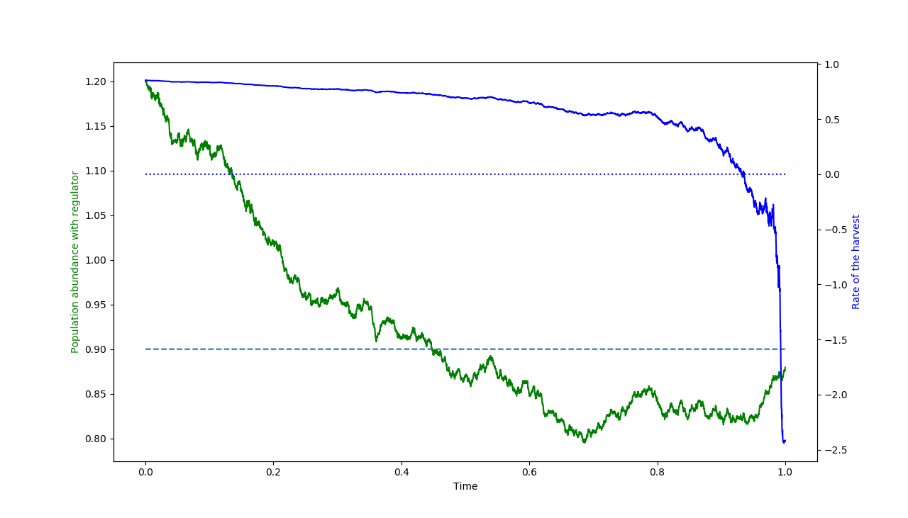
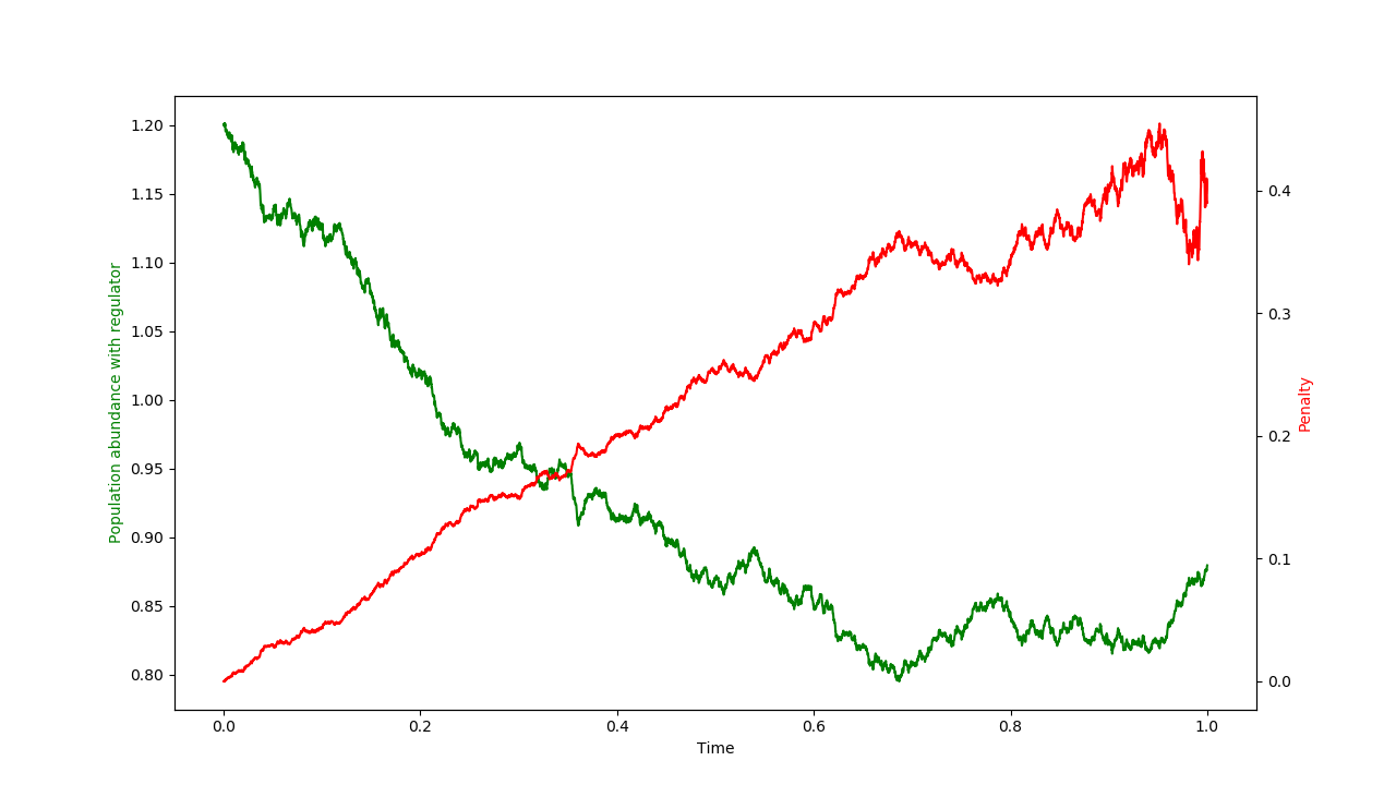
Refer to caption
Figure 3: A trajectory of the optimally controlled population abundance (green curve, y𝑦y-axis on the left) and the associated optimal harvest rate (blue curve, y𝑦y-axis on the right) w.r.t. the time (x𝑥x-axis). The dotted line corresponds to α=0𝛼0\alpha=0, and the dashed line corresponds to Xtα=βsuperscriptsubscript𝑋𝑡superscript𝛼𝛽X_{t}^{\alpha^{*}}=\beta.
Refer to caption
Figure 4: The evolution of the penalty (y𝑦y-axis on the right, red curve) and the population abundance (y𝑦y-axis on the left, green curve) w.r.t. the time (x𝑥x-axis).

Figure 4 shows that the Agent harvests with an important rate at the beginning : αtsubscript𝛼𝑡\alpha_{t} is around 0.60.60.6. As he get closer to the matirity, the Agent slows down the harvest and then renew the resource. This can be interpreted as follows.

The Agent harvests with a high rate and do note care about the tax at maturity since the population as has time to regenerate itself.

Getting closer to the maturity, the Agent take into acount the tax and slows down the harvest. When very close to maturity, t0.93𝑡0.93t\approx 0.93, the Agent renews the population to ensure an abundance close to the target β=0.9𝛽0.9\beta=0.9 to limit the tax. This shows that the incentive policy is efficient.

Figure 4 presents the forecast of the penalty (i.e. YR~,Zε,nsuperscript𝑌~𝑅superscript𝑍𝜀𝑛Y^{\tilde{R},Z^{\varepsilon},n}) in red, and the abundance population in green. We notice these two quantities evolve in opposite ways: for high values of the abundance, the expected tax is low, and for low abundance the penalty becomes greater.

We now study the sensitivity of the incentive policy w.r.t. the target β𝛽\beta (see Figure 6) and w.r.t. the renewal cost c𝑐c (see Figure 6).

Refer to caption
Figure 5: Evolution in mean of the population abundance w.r.t. the time for different values of β𝛽\beta.
Refer to caption
Figure 6: Evolution in mean of the population abundance w.r.t. the time for different values of c𝑐c.

Figure 6 presents the evolution in mean of the abundance w.r.t. time for several values of β𝛽\beta. The mean is approximated by the empirical mean over 1000 trajectories. We remark that at each time the mean of the population abundance is more important as β𝛽\beta is larger. This shows that the choice of β𝛽\beta influences the behavior of the resource manager: the most is important β𝛽\beta the least the Agent harvests. We also notice that for each value of β𝛽\beta, the mean terminal value reaches the target, which also shows the incentive effect of the parameter β𝛽\beta.

Figure 6 shows the evolution of the mean of the resource abundance w.r.t. time for several values of the costs parameter c𝑐c. The mean is approximated by the empirical mean over for 1000 trajectories. We remark that the population abundance is nondecreasing w.r.t. c𝑐c. In particular, the highest the penalty is, the most the Agent is concerned, through the incentive policy, by the size of the population at the end.

We now compare the situation for which the Agent can renew the population abundance (that is M¯>0¯𝑀0\underline{M}>0) with the situation for which the Agent can only harvest (that is M¯=0¯𝑀0\underline{M}=0).

Refer to caption
Figure 7: Evolution in mean of the population abundance w.r.t. the time when the Agent can (blue curve) and cannot (orange curve) renew the population abundance.

In Figure 7 the mean is approximated by the empirical mean over 1000 trajectories. We remark that at each time the population abundance is more important in mean if the Agent cannot renew the resource. Indeed, if the resource is not renewable, the Agent reduces his harvesting rate in prevision of the terminal tax. On the contrary, if the resource can be renewed, the Agent harvests more to generate a higher profit since he can reduce the terminal tax by renewing the resource at the end.

Appendix A Proof of Proposition 4.1

We first recall that {\cal H} is defined by

(y,δ1,δ2)𝑦subscript𝛿1subscript𝛿2\displaystyle\mathcal{H}(y,\delta_{1},\delta_{2}) =\displaystyle= supz{eyp(ey)a(ey,z)a(ey,z)22σ22γz2+(λσ22μ(ey)a(ey,z))δ1}subscriptsupremum𝑧superscript𝑒𝑦𝑝superscript𝑒𝑦superscript𝑎superscript𝑒𝑦𝑧superscript𝑎superscriptsuperscript𝑒𝑦𝑧22superscript𝜎22𝛾superscript𝑧2𝜆superscript𝜎22𝜇superscript𝑒𝑦superscript𝑎superscript𝑒𝑦𝑧subscript𝛿1\displaystyle\sup_{z\in\mathbb{R}}\left\{e^{y}p(e^{y})a^{*}(e^{y},z)-{a^{*}(e^{y},z)^{2}\over 2}-\frac{\sigma^{2}}{2}\gamma z^{2}+(\lambda-{\sigma^{2}\over 2}-\mu(e^{y})-a^{*}(e^{y},z))\delta_{1}\right\}
+σ22δ2,(y,δ1,δ2)××.superscript𝜎22subscript𝛿2𝑦subscript𝛿1subscript𝛿2\displaystyle+\frac{\sigma^{2}}{2}\delta_{2}\;,\quad(y,\delta_{1},\delta_{2})\in\mathbb{R}\times\mathbb{R}\times\mathbb{R}\;.

From the definition of asuperscript𝑎a^{*} given in (3.7) we can rewrite {\cal H} by considering the different cases eyp(ey)+z<M¯superscript𝑒𝑦𝑝superscript𝑒𝑦𝑧¯𝑀e^{y}p(e^{y})+z<-\underline{M}, M¯eyp(ey)+zM¯¯𝑀superscript𝑒𝑦𝑝superscript𝑒𝑦𝑧¯𝑀-\underline{M}\leq e^{y}p(e^{y})+z\leq\overline{M} and eyp(ey)+z>M¯superscript𝑒𝑦𝑝superscript𝑒𝑦𝑧¯𝑀e^{y}p(e^{y})+z>\overline{M}, and making the variable change zeyp(ey)𝑧superscript𝑒𝑦𝑝superscript𝑒𝑦z-e^{y}p(e^{y}) for z𝑧z under the following form

(y,δ1,δ2)𝑦subscript𝛿1subscript𝛿2\displaystyle\mathcal{H}(y,\delta_{1},\delta_{2}) =\displaystyle= max{𝒦1(y,δ1),𝒦2(y,δ1),𝒦3(y,δ1)}+(λσ22μ(ey))δ1+σ22δ2,subscript𝒦1𝑦subscript𝛿1subscript𝒦2𝑦subscript𝛿1subscript𝒦3𝑦subscript𝛿1𝜆superscript𝜎22𝜇superscript𝑒𝑦subscript𝛿1superscript𝜎22subscript𝛿2\displaystyle\max\Big{\{}\mathcal{K}_{1}(y,\delta_{1}),\mathcal{K}_{2}(y,\delta_{1}),\mathcal{K}_{3}(y,\delta_{1})\Big{\}}+(\lambda-\frac{\sigma^{2}}{2}-\mu(e^{y}))\delta_{1}+\frac{\sigma^{2}}{2}\delta_{2}\;,

where

𝒦1(y,δ1)subscript𝒦1𝑦subscript𝛿1\displaystyle\mathcal{K}_{1}(y,\delta_{1}) =\displaystyle= supzM¯{(δ1eyp(ey)M¯2)M¯σ22γ(zeyp(ey))2}subscriptsupremum𝑧¯𝑀subscript𝛿1superscript𝑒𝑦𝑝superscript𝑒𝑦¯𝑀2¯𝑀superscript𝜎22𝛾superscript𝑧superscript𝑒𝑦𝑝superscript𝑒𝑦2\displaystyle\sup_{z\leq-\underline{M}}\left\{\left(\delta_{1}-e^{y}p(e^{y})-{\underline{M}\over 2}\right)\underline{M}-{\sigma^{2}\over 2}\gamma\left(z-e^{y}p(e^{y})\right)^{2}\right\}
=\displaystyle= (δ1eyp(ey)M¯2)M¯σ22γ(M¯+eyp(ey))2,subscript𝛿1superscript𝑒𝑦𝑝superscript𝑒𝑦¯𝑀2¯𝑀superscript𝜎22𝛾superscript¯𝑀superscript𝑒𝑦𝑝superscript𝑒𝑦2\displaystyle\left(\delta_{1}-e^{y}p(e^{y})-{\underline{M}\over 2}\right)\underline{M}-{\sigma^{2}\over 2}\gamma\left(\underline{M}+e^{y}p(e^{y})\right)^{2}\;,
𝒦2(y,δ1)subscript𝒦2𝑦subscript𝛿1\displaystyle\mathcal{K}_{2}(y,\delta_{1}) =\displaystyle= supzM¯{(δ1eyp(ey)M¯2)M¯σ22γ(zeyp(ey))2}subscriptsupremum𝑧¯𝑀subscript𝛿1superscript𝑒𝑦𝑝superscript𝑒𝑦¯𝑀2¯𝑀superscript𝜎22𝛾superscript𝑧superscript𝑒𝑦𝑝superscript𝑒𝑦2\displaystyle\sup_{z\geq\overline{M}}\left\{\left(\delta_{1}-e^{y}p(e^{y})-{\overline{M}\over 2}\right)\overline{M}-{\sigma^{2}\over 2}\gamma\left(z-e^{y}p(e^{y})\right)^{2}\right\}
=\displaystyle= (δ1+eyp(ey)M¯2)M¯σ22γ([M¯eyp(ey)]+)2,subscript𝛿1superscript𝑒𝑦𝑝superscript𝑒𝑦¯𝑀2¯𝑀superscript𝜎22𝛾superscriptsubscriptdelimited-[]¯𝑀superscript𝑒𝑦𝑝superscript𝑒𝑦2\displaystyle\left(-\delta_{1}+e^{y}p(e^{y})-{\overline{M}\over 2}\right)\overline{M}-{\sigma^{2}\over 2}\gamma\left(\left[\overline{M}-e^{y}p(e^{y})\right]_{+}\right)^{2}\;,

and

𝒦3(y,δ1)=supM¯zM¯{12(1+γσ2)z2+(eyp(ey)(1+γ2σ)δ1)z}σ22γ|eyp(ey)|2subscript𝒦3𝑦subscript𝛿1subscriptsupremum¯𝑀𝑧¯𝑀121𝛾superscript𝜎2superscript𝑧2superscript𝑒𝑦𝑝superscript𝑒𝑦1superscript𝛾2𝜎subscript𝛿1𝑧superscript𝜎22𝛾superscriptsuperscript𝑒𝑦𝑝superscript𝑒𝑦2\mathcal{K}_{3}(y,\delta_{1})=\sup_{-\underline{M}\leq z\leq\overline{M}}\left\{-{1\over 2}(1+\gamma\sigma^{2})z^{2}+\big{(}e^{y}p(e^{y})(1+\gamma^{2}\sigma)-\delta_{1}\big{)}z\right\}-\frac{\sigma^{2}}{2}\gamma|e^{y}p(e^{y})|^{2}

for all y,δ1𝑦subscript𝛿1y,\delta_{1}\in\mathbb{R}.

A straightforward computation gives 𝒦3(y,δ1)=Q(eyp(ey),δ1)subscript𝒦3𝑦subscript𝛿1𝑄superscript𝑒𝑦𝑝superscript𝑒𝑦subscript𝛿1\mathcal{K}_{3}(y,\delta_{1})=Q(e^{y}p(e^{y}),\delta_{1}) where

Q(𝔭,δ1)𝑄𝔭subscript𝛿1\displaystyle Q(\mathfrak{p},\delta_{1}) =\displaystyle= (𝔭(1+γ2σ)δ1)22(1+γσ2)𝟙𝔭δ11+γσ2[M¯,M¯]superscript𝔭1superscript𝛾2𝜎subscript𝛿1221𝛾superscript𝜎2subscript1𝔭subscript𝛿11𝛾superscript𝜎2¯𝑀¯𝑀\displaystyle{\big{(}\mathfrak{p}(1+\gamma^{2}\sigma)-\delta_{1}\big{)}^{2}\over 2(1+\gamma\sigma^{2})}\mathds{1}_{\mathfrak{p}-{\delta_{1}\over 1+\gamma\sigma^{2}}\in[-\underline{M},\overline{M}]}
+(12(1+γσ2)M¯2+(𝔭(1+γ2σ)δ1)M¯)𝟙𝔭δ11+γσ2(M¯,+)121𝛾superscript𝜎2superscript¯𝑀2𝔭1superscript𝛾2𝜎subscript𝛿1¯𝑀subscript1𝔭subscript𝛿11𝛾superscript𝜎2¯𝑀\displaystyle+\left(-{1\over 2}(1+\gamma\sigma^{2})\overline{M}^{2}+\big{(}\mathfrak{p}(1+\gamma^{2}\sigma)-\delta_{1}\big{)}\overline{M}\right)\mathds{1}_{\mathfrak{p}-{\delta_{1}\over 1+\gamma\sigma^{2}}\in(\overline{M},+\infty)}
+(12(1+γσ2)M¯2(𝔭(1+γ2σ)δ1)M¯)𝟙𝔭δ11+γσ2(,M¯)121𝛾superscript𝜎2superscript¯𝑀2𝔭1superscript𝛾2𝜎subscript𝛿1¯𝑀subscript1𝔭subscript𝛿11𝛾superscript𝜎2¯𝑀\displaystyle+\left(-{1\over 2}(1+\gamma\sigma^{2})\underline{M}^{2}-\big{(}\mathfrak{p}(1+\gamma^{2}\sigma)-\delta_{1}\big{)}\underline{M}\right)\mathds{1}_{\mathfrak{p}-{\delta_{1}\over 1+\gamma\sigma^{2}}\in(-\infty,-\underline{M})}
σ22γ|𝔭|2superscript𝜎22𝛾superscript𝔭2\displaystyle-\frac{\sigma^{2}}{2}\gamma|\mathfrak{p}|^{2}

for all 𝔭,δ1𝔭subscript𝛿1\mathfrak{p},\delta_{1}\in\mathbb{R}.

We then introduce the functions absε:+:subscriptabs𝜀subscript\mathrm{abs}_{\varepsilon}:~{}\mathbb{R}\rightarrow\mathbb{R}_{+} and maxε:2:subscript𝜀superscript2\max_{\varepsilon}:~{}\mathbb{R}^{2}\rightarrow\mathbb{R} defined by

absε(x)subscriptabs𝜀𝑥\displaystyle\mathrm{abs}_{\varepsilon}(x) =\displaystyle= |x|(Θ(4εx3)+Θ(4εx3)),x,𝑥Θ4𝜀𝑥3Θ4𝜀𝑥3𝑥\displaystyle|x|\Big{(}\Theta\Big{(}-\frac{4}{\varepsilon}x-3\Big{)}+\Theta\Big{(}\frac{4}{\varepsilon}x-3\Big{)}\Big{)}\;,\quad x\in\mathbb{R}\;,
maxε(x,y)subscriptmax𝜀𝑥𝑦\displaystyle\mathrm{max}_{\varepsilon}(x,y) =\displaystyle= absε(xy)+x+y2,x,y,subscriptabs𝜀𝑥𝑦𝑥𝑦2𝑥𝑦\displaystyle{\mathrm{abs}_{\varepsilon}(x-y)+x+y\over 2}\;,\quad x,y\in\mathbb{R}\;,

for any ε>0𝜀0\varepsilon>0 where we recall that the function ΘΘ\Theta is defined by (4.25). From the definition of ΘΘ\Theta, the function maxεsubscriptmax𝜀\mathrm{max}_{\varepsilon} is infinitely differentiable with bounded derivatives and we have

supx,y|max(x,y)maxε(x,y)|subscriptsupremum𝑥𝑦𝑥𝑦subscriptmax𝜀𝑥𝑦\displaystyle\sup_{x,\,y\,\in\,\mathbb{R}}\big{|}\max(x,y)-\mathrm{max}_{\varepsilon}(x,y)\big{|} \displaystyle\leq ε3𝜀3\displaystyle{\varepsilon\over 3} (A.37)

for all ε>0𝜀0\varepsilon>0.

Fix the constant Γ:=max{M¯(1+γσ2),(P+M¯)(1+γσ2)}assignΓ¯𝑀1𝛾superscript𝜎2𝑃¯𝑀1𝛾superscript𝜎2\Gamma:=\max\left\{\overline{M}(1+\gamma\sigma^{2}),(P+\underline{M})(1+\gamma\sigma^{2})\right\}. Since the function Q𝑄Q is continuous on 2superscript2\mathbb{R}^{2}, there exists Qεsubscript𝑄𝜀Q_{\varepsilon} infinitely differentiable on 2superscript2\mathbb{R}^{2} such that

sup(𝔭,δ1)[0,P]×[(Γ+1),Γ+1]|Q(𝔭,δ1)Qε(𝔭,δ1)|subscriptsupremum𝔭subscript𝛿10𝑃Γ1Γ1𝑄𝔭subscript𝛿1subscript𝑄𝜀𝔭subscript𝛿1\displaystyle\sup_{(\mathfrak{p},\delta_{1})\in[0,P]\times[-(\Gamma+1),\;\Gamma+1]}|Q(\mathfrak{p},\delta_{1})-Q_{\varepsilon}(\mathfrak{p},\delta_{1})| \displaystyle\leq ε3.𝜀3\displaystyle{\varepsilon\over 3}\;. (A.38)

We then define 𝒦3,εsubscript𝒦3𝜀{\cal K}_{3,\varepsilon} for any y,δ1𝑦subscript𝛿1y,\delta_{1}\in\mathbb{R} by

𝒦3,ε(y,δ1)subscript𝒦3𝜀𝑦subscript𝛿1\displaystyle{\cal K}_{3,\varepsilon}(y,\delta_{1}) =\displaystyle= Qε(eyp(ey),δ1)(1Θ(2(δ1Γ)1)Θ(2(Γ+δ1)1)))\displaystyle Q_{\varepsilon}(e^{y}p(e^{y}),\delta_{1}){\Big{(}1-\Theta(2(\delta_{1}-\Gamma)-1)-\Theta\big{(}-2(\Gamma+\delta_{1})-1)\big{)}\Big{)}}
+(12(1+γσ2)M¯2(eyp(ey)(1+γ2σ)δ1)M¯)Θ(2(δ1Γ)1)121𝛾superscript𝜎2superscript¯𝑀2superscript𝑒𝑦𝑝superscript𝑒𝑦1superscript𝛾2𝜎subscript𝛿1¯𝑀Θ2subscript𝛿1Γ1\displaystyle+\left(-{1\over 2}(1+\gamma\sigma^{2})\underline{M}^{2}-\big{(}e^{y}p(e^{y})(1+\gamma^{2}\sigma)-\delta_{1}\big{)}\underline{M}\right){\Theta\big{(}2(\delta_{1}-\Gamma)-1\big{)}}
+(12(1+γσ2)M¯2+(eyp(ey)(1+γ2σ)δ1)M¯)Θ(2(Γ+δ1)1).121𝛾superscript𝜎2superscript¯𝑀2superscript𝑒𝑦𝑝superscript𝑒𝑦1superscript𝛾2𝜎subscript𝛿1¯𝑀Θ2Γsubscript𝛿11\displaystyle+\left(-{1\over 2}(1+\gamma\sigma^{2})\overline{M}^{2}+\big{(}e^{y}p(e^{y})(1+\gamma^{2}\sigma)-\delta_{1}\big{)}\overline{M}\right){\Theta\big{(}-2(\Gamma+\delta_{1})-1\big{)}}\;.

From (A.38) we have

sup2|𝒦3,ε𝒦3|ε3.subscriptsupremumsuperscript2subscript𝒦3𝜀subscript𝒦3𝜀3\sup_{\mathbb{R}^{2}}|\mathcal{K}_{3,\varepsilon}-\mathcal{K}_{3}|\leq{\varepsilon\over 3}\;.

We then define for any y,δ1,δ2𝑦subscript𝛿1subscript𝛿2y,\delta_{1},\delta_{2}\in\mathbb{R} the approximated Hamiltonian εsubscript𝜀{\cal H}_{\varepsilon} by

ε(y,δ1,δ2):=maxε{𝒦1(y,δ1),𝒦2(y,δ1),𝒦3,ε(y,δ1)}+σ22δ2+(λσ22μ(ey))δ1.assignsubscript𝜀𝑦subscript𝛿1subscript𝛿2subscriptmax𝜀subscript𝒦1𝑦subscript𝛿1subscript𝒦2𝑦subscript𝛿1subscript𝒦3𝜀𝑦subscript𝛿1superscript𝜎22subscript𝛿2𝜆superscript𝜎22𝜇superscript𝑒𝑦subscript𝛿1\mathcal{H}_{\varepsilon}(y,\delta_{1},\delta_{2}):=\mathrm{max}_{\varepsilon}\Big{\{}\mathcal{K}_{1}(y,\delta_{1}),\mathcal{K}_{2}(y,\delta_{1}),\mathcal{K}_{3,\varepsilon}(y,\delta_{1})\Big{\}}+\frac{\sigma^{2}}{2}\delta_{2}+(\lambda-\frac{\sigma^{2}}{2}-\mu(e^{y}))\delta_{1}\;.

We therefore get from (A.37)

sup3|ε|ε.subscriptsupremumsuperscript3subscript𝜀𝜀\sup_{\mathbb{R}^{3}}|\mathcal{H}_{\varepsilon}-\mathcal{H}|\leq\varepsilon\;.

We then turn the PDE driven by εsubscript𝜀{\cal H}_{\varepsilon} that writes

{twεε(y,ywε(t,y),yywε(t,y))=0,(t,y)[0,T)×,wε(T,y)=f(ey),y.casesotherwiseformulae-sequencesubscript𝑡subscript𝑤𝜀subscript𝜀𝑦subscript𝑦subscript𝑤𝜀𝑡𝑦subscript𝑦𝑦subscript𝑤𝜀𝑡𝑦0𝑡𝑦0𝑇otherwiseformulae-sequencesubscript𝑤𝜀𝑇𝑦𝑓superscript𝑒𝑦𝑦\begin{cases}&-\partial_{t}w_{\varepsilon}-\mathcal{H}_{\varepsilon}\Big{(}y,\partial_{y}w_{\varepsilon}(t,y),\partial_{yy}w_{\varepsilon}(t,y)\Big{)}=0\;,\quad(t,y)\in[0,T)\times\mathbb{R}\;,\\ &w_{\varepsilon}(T,y)=-f(e^{y})\;,\quad y\in\mathbb{R}\;.\end{cases} (A.39)

Under Assumption (H’), we can write the approximated Hamiltonian 3,εsubscript3𝜀{\cal H}_{3,\varepsilon} under the form

3,ε(y,δ1,δ2)=σ22δ2+bε(u,δ1)δ1+cε(y,δ1)subscript3𝜀𝑦subscript𝛿1subscript𝛿2superscript𝜎22subscript𝛿2subscript𝑏𝜀𝑢subscript𝛿1subscript𝛿1subscript𝑐𝜀𝑦subscript𝛿1{\cal H}_{3,\varepsilon}(y,\delta_{1},\delta_{2})=\frac{\sigma^{2}}{2}\delta_{2}+b_{\varepsilon}(u,\delta_{1})\delta_{1}+c_{\varepsilon}(y,\delta_{1})

where the coefficients bεsubscript𝑏𝜀b_{\varepsilon} and cεsubscript𝑐𝜀c_{\varepsilon} satisfy Conditions A, B and D of [22]. Then, according to Theorem 14 in [22], PDE (A.39) admits a unique solution wεC2+ν([0,T]×)subscript𝑤𝜀superscript𝐶2𝜈0𝑇w_{\varepsilon}\in C^{2+\nu}([0,T]\times\mathbb{R}).

References

  • [1] Robert Almgren, Chee Thum, Emmanuel Hauptmann, and Hong Li. Equity market impact. Risk, 18:58–62, 2003.
  • [2] Luis HR Alvarez and Erkki Koskela. Optimal harvesting under resource stock and price uncertainty. Journal of Economic Dynamics and Control, 31(7):2461–2485, 2007.
  • [3] Kenneth Arrow. Research in management controls: a critical synthesis. Management Controls: New Directions in Basic Research, pages 317–327, 1964.
  • [4] Kenneth J Arrow. The theory of risk aversion. Essays in the theory of risk-bearing, pages 90–120, 1971.
  • [5] Edward B. Barbier. The role of economic incentives for natural resource economic progress and environmental concerns. pages 153–178. A Publications of the Egon-Sohmen-Foundation. Springer, Berlin, Heidelberg, 1993.
  • [6] Philippe Briand and Ying Hu. Bsde with quadratic growth and unbounded terminal value. Probability Theory and Related Fields, 136(4):604–618, 2006.
  • [7] Colin W Clark. Profit maximization and the extinction of animal species. Journal of Political Economy, 81(4):950–961, 1973.
  • [8] Jakša Cvitanić, Dylan Possamaï, and Nizar Touzi. Moral hazard in dynamic risk management. Management Science, 63(10):3328–3346, 2016.
  • [9] Jakša Cvitanić, Dylan Possamaï, and Nizar Touzi. Dynamic programming approach to princial–agent problems. Finance and Stochastics, 22(1):1–37, 2018.
  • [10] Nicole El Karoui, Shige Peng, and Marie Claire Quenez. Backward stochastic differential equations in finance. Mathematical finance, 7(1):1–71, 1997.
  • [11] Eurostat. Sustainable development in the european union. Technical report, 2018 Edition.
  • [12] Steven N Evans, Alexandru Hening, and Sebastian J Schreiber. Protected polymorphisms and evolutionary stability of patch-selection strategies in stochastic environments. Journal of mathematical biology, 71(2):325–359, 2015.
  • [13] Gérard Gaudet and Pierre Lasserre. The management of natural resources under asymmetry of information. Annu. Rev. Resour. Econ., 7(1):291–308, 2015.
  • [14] Heidi Gjertsen and Eduard Niesten. Incentive-based approaches in marine conservation: applications for sea turtles. Conservation and Society, 8(1):5–14, 2010.
  • [15] R Quentin Grafton, Ragnar Arnason, Trond Bjørndal, David Campbell, Harry F Campbell, Colin W Clark, Robin Connor, Diane P Dupont, Rögnvaldur Hannesson, Ray Hilborn, et al. Incentive-based approaches to sustainable fisheries. Canadian Journal of Fisheries and Aquatic Sciences, 63(3):699–710, 2006.
  • [16] Bengt Holmstrom and Paul Milgrom. Aggregation and linearity in the provision of intertemporal incentives. Econometrica: Journal of the Econometric Society, pages 303–328, 1987.
  • [17] Ying Hu, Peter Imkeller, Matthias Müller, et al. Utility maximization in incomplete markets. The Annals of Applied Probability, 15(3):1691–1712, 2005.
  • [18] Ioannis Karatzas and Steven E Shreve. BrownianMotionandStochasticCalculus, volume 113 of Gradute Texts in Mathematics. Springer, second edition edition, 1998.
  • [19] Nicolai V. Krylov. Controlled Diffusion Processes, volume 14 of Application of Mathematics. Springer, 1980.
  • [20] Fabrizio Lillo, J. Doyne Farmer, and Rosario N. Mantagna. Master curve for price impact function. Nature, 421:129–130, 2003.
  • [21] Sylvie Méléard and Vincent Bansaye. Some stochastic models for structured populations: scaling limits and long time behavior. arXiv preprint arXiv:1506.04165 v1, 2015.
  • [22] Olga Arsen’evna Oleinik and Stanislav Nikolaevich Kruzhkov. Quasi-linear second-order parabolic equations with many independent variables. Russian Mathematical Surveys, 16(5):105–146, 1961.
  • [23] Stephen A Ross. The economic theory of agency: The principal’s problem. The American economic review, 63(2):134–139, 1973.
  • [24] Richard Rouge and Nicole El Karoui. Pricing via utility maximization and entropy. Mathematical Finance, 10(2):259–276, 2000.
  • [25] Yuliy Sannikov. A continuous-time version of the principal-agent problem. The Review of Economic Studies, 75(3):957–984, 2008.
  • [26] Helen Suich. The effectiveness of economic incentives for sustaining community based natural resource management. Land Use Policy, 31:441–449, 2013.
  • [27] Fleming Wendell H. and H. M. Soner. Controlled Markov Processes and Viscosity Solutions, volume 25 of Stochastic Modelling and Applied Probability. Springer, second edition edition, 2006.
  • [28] Robert Wilson. The theory of syndicates. Econometrica: journal of the Econometric Society, pages 119–132, 1968.
  • [29] Robert B Wilson. The structure of incentives for decentralization under uncertainty. Number 121. Graduate School of Business, Stanford University, 1967.