A whole-year simulation study on nonlinear mixed-integer model predictive control for a thermal energy supply system with multi-use components

Abstract

This work presents a whole-year simulation study on nonlinear mixed-integer Model Predictive Control (MPC) for a complex thermal energy supply system which consists of a heat pump, stratified water storages, free cooling facilities, and a large underground thermal storage. For solution of the arising Mixed-Integer Non-Linear Programs (MINLPs) we apply an existing general and optimal-control-suitable decomposition approach. To compensate deviation of forecast inputs from measured disturbances, we introduce a moving horizon estimation step within the MPC strategy. The MPC performance for this study, which consists of more than 50,000 real time suitable MINLP solutions, is compared to an elaborate conventional control strategy for the system. It is shown that MPC can significantly reduce the yearly energy consumption while providing a similar degree of constraint satisfaction, and autonomously identify previously unknown, beneficial operation modes.

1 Introduction

The transition towards a sustainable energy system requires a substantial contribution in the buildings sector, which is responsible for approximately 40 % of the energy consumption in the EU (Berardi, 2017). Low-energy buildings enable efficient utilization of provided thermal energy and, in combination with thermal component activation, facilitate the deployment of free cooling and efficient use of heat pumps. An intelligent mix of heat sources and sinks in combination with smart storage management can increase the efficiency of these systems considerably, cf. Hesaraki et al. (2015). However, such configurations might incorporate numerous operating modes and states, which makes it difficult to identify and implement conventional, rule-based control strategies that are able to determine the most efficient operating mode at any given time point.

During recent years, a strand of literature has built which shows that MPC is well suited for control of energy systems. The incorporation of models and forecasts allows for efficient machinery utilization as well as situation-dependent, predictive control decisions, and renders MPC well suited for systems governed by slow dynamics and/or large delays. Successful applications can be found for a variety of systems, such as heat pump systems (Fischer et al., 2017; Baeten et al., 2017), district heating systems (Dainese et al., 2019) and microgrids (Zachar and Daoutidis, 2019; Iovine et al., 2019).

Due to switching behavior of components such as heat pumps, combined heat and power plants etc., application of MPC for energy systems often requires the solution of mixed-integer optimization problems on real time suitable time scales. Therefore, according optimization problems are often formulated as either Mixed-Integer Linear Programs (MILPs) as in Bianchini et al. (2019) and Lv et al. (2019), or Mixed-Integer Quadratic Programs (MIQPs) as in Vasallo and Bravo (2016) and Killian et al. (2018), using linear(ized) models for system modeling.

However, the underlying processes are often characterized by nonlinear correlations, so that the utilization of nonlinear models for mixed-integer MPC can improve the accuracy of system descriptions, and with this, the quality of control decisions. The solution of the arising Mixed-Integer Non-Linear Programs (MINLPs) on suitable time scales remains a challenging task though, which for non-trivial problems can only be achieved approximately, cf. Schweiger et al. (2017), Dias et al. (2018), Kuboth et al. (2019).

Within this work, we show a successful application of a general, optimal-control-suitable approach for approximate MINLP solution by Sager (2009), Sager et al. (2011) within a whole-year simulation study for mixed-integer MPC of the nonlinear model of a complex thermal energy supply system. The system consists of a Heat Pump (HP), stratified water storages, free cooling facilities, and a large underground thermal storage. Model nonlinearities arise, amongst others, from consideration of mass flow rates as continuous controls of the system as well as nonlinear Coefficient Of Performance (COP) computations for the HP, which further introduces switching behavior due to minimal part load. Since the quality of utilized forecasts highly influences performance (cf. Oldewurtel et al. (2012)), we introduce a Moving Horizon Estimation (MHE) step for online correction of forecasts within the MPC strategy to compensate deviation of forecasted inputs from measured disturbances. The performance of the MPC strategy applied for this study, which consists of more than 50,000 real time suitable MINLPs solutions, is compared to an elaborate, conventional control strategy for the system.

The contributions of this paper are as follows. First, the use of techniques for reduction of nonlinearities and elimination of discontinuities on modeling of real-life sized energy systems for later application within derivative-based optimization methods are demonstrated. Then, the developed models are applied within an integrated approach for simulation of a complete MPC-MHE loop for a nonlinear switched thermal energy system. The methods applied for solving the arising MINLPs are general and suitable not only for simulation, but also for real-time control applications of physical systems. Finally, it its shown within a case study that the MPC is capable not only to significantly reduce the yearly energy consumption while providing a similar degree of constraint satisfaction, but also to identify beneficial operation modes which have not been identified before by the designers of the conventional controller.

The remainder of this paper is organized as follows. The system subject to this study is introduced in Section 2, while Section 3 presents the chosen modeling approach. The elaborate conventional control strategy is introduced in Section 4 and the MPC strategy in Section 5. The performance of the applied control strategies is compared within a simulation study in Section 6, followed by a conclusion and outlook in Section 7.

2 System description

In the following, a description of the system subject to this study is given by introducing its components, function principles, operation modes and limits.

Figure 1: Schematic depiction of the thermal energy supply system considered within this study: green boxes indicates controllable quantities, orange boxes indicate time-varying parameters determined by external factors. Red arrows indicate the main energy flows across the system boundaries.

2.1 System components

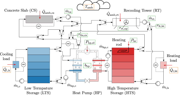
This study is inspired by an innovative thermal energy supply system for an office building under construction in Karlsruhe, Germany. The system variant and model used within this work originated from a research project of Ottensmeier Ingenieure GmbH, Paderborn and Karlsruhe University of Applied Sciences focused on the dimensioning of system components and control design for the physical system.

An overview of the system considered within this study and the possible interactions between its components is given in Figure 1. One key component of the system is a Concrete Slab (CS) which is located below surface level of the building. This component, which assembles the underground parking deck of the building, is thermally activated through encased tubes within the concrete. These tubes with diameter $d_{\mathrm{t,rc}}=2.62\,\mathrm{cm}$ are embedded as $n_{\mathrm{cs}}=306$ identical Reinforcement Cages (RCs), exemplary shown in Figure 2. Each cage is $w_{\mathrm{rc}}=0.5\,\mathrm{m}$ wide, $h_{\mathrm{rc}}=1.1\,\mathrm{m}$ high, $l_{\mathrm{rc}}=9.0\,\mathrm{m}$ long and contains three layers of pipe loop with a total tube length of 58 m per cage. Hydraulically, all cages are connected in parallel. The bottom of the CS rests on soil, the top of the CS is exposed to the air in the underground car park.

Figure 2: Schematic depiction of one of the reinforcement cages that build the underground concrete slab.

Further, two stratified water storages are installed: a Low Temperature Storage (LTS) with a volume of $V_{\mathrm{lts}}=10.0\,\mathrm{m}^{3}$ and a High Temperature Storage (HTS) with a volume of $V_{\mathrm{hts}}=5.0\,\mathrm{m}^{3}$. Connected to these is a HP with a maximum electric compressor power of $P_{\mathrm{hp,el,max}}=60\,\mathrm{kW}$. Additionally, the HTS is equipped with electrical Heating Rods (HRs) with total maximum heating power $P_{\mathrm{hr,max}}=400\,\mathrm{kW}$ intended as backup heating devices. Outside of the building, a Recooling Tower (RT) with total heat exchange area $A_{\mathrm{rt}}=2145.0\,\mathrm{m}^{2}$, fluid volume $V_{\mathrm{rt}}=0.208\,\mathrm{m}^{3}$ and heat transfer coefficient $\alpha_{\mathrm{rt}}=21.6\,\mathrm{W}/\mathrm{K}$ is installed and connected to the indoor components. While the heating and cooling demands of the building on the one hand strongly depend on the current ambient temperature and solar irradiation, additional constant cooling demands arise from a number of server computers operated in the building.

Multiple temperature sensors are installed inside CS, storages and RT as well as at their corresponding inlets and outlets. Additionally, five Heat Meters (HMs) are installed in selected positions to enable monitoring and improved control decisions.

2.2 Interaction of components

The LTS is the heat source for the HP. When the HP is active, water is extracted from the top of the LTS and returned to the bottom of the storage with reduced temperature. From the bottom of the LTS, water is extracted to cover cooling loads, resulting in water with increased temperature returning to the top of the storage.

Accordingly, the HTS is the heat sink of the HP, which extracts water from the bottom and returns it to the top of the storage with increased temperature. From the top of the HTS, water is extracted to cover heating loads, resulting in water with reduced temperature returning to the bottom of the storage. The temperature of the HTS can additionally be increased using the HRs.

Medium from both storages can be supported to the outdoor RT for heat exchange with the ambient air. Depending on current ambient temperature and operation level of the RT, this allows to either cool down the LTS in free cooling mode, or to heat up the LTS when acting as a heat source for the HP. On the other hand, the RT can be utilized for cooling of the HTS which enables the HTS to act as recooling for the HP.

Further, water from the LTS can be transferred through the CS to either reduce or increase the temperature inside of the LTS, so that the CS acts as both heat source and heat sink for the LTS. Additionally, a splitter installed behind the RT can be utilized to affect how much of the medium flowing through the RT is led to the LTS and how much is led into the CS.

2.3 Controls, operation limits and parameters

Within this study, we assume that the mass flow $\dot{m}_{\mathrm{rt}}$ of the RT pump and the mass flow $\dot{m}_{\mathrm{cs}}$ of the CS pump can be chosen directly and on a continuous scale. Control $r_{\mathrm{rt,op}}$ sets the operation level of the RT. The control $r_{\mathrm{lt,ht}}$ depicts a mixing valve which influences how much of the mass flow through the RT is supported towards the Low Temperature (LT) side of the system, while the remaining fraction is supported towards the High Temperature (HT) side. Control $r_{\mathrm{lts,cs}}$ is an additional mixing valve to determine how much of the medium flowing from the RT to the LT side is supported to the LTS, while the remaining fraction is supported to the CS.

The HP can be activated using a binary switch $b_{\mathrm{hp}}$. Once the machine is turned on, it is assumed to operate with minimum part load $P_{\mathrm{hp,el,min}}=2.0\,\mathrm{kW}$. From that, the electrical power $P_{\mathrm{hp,el}}$ of the HP can be modulated continuously. The power of the HRs can be chosen on a continuous scale. A summary of all controls is given in Table 1.

Control	Type	Minimum	Maximum
$\dot{m}_{\mathrm{rt}}$	continuous	$0.0\,\mathrm{kg/s}$	$200.0\,\mathrm{kg/s}$
$\dot{m}_{\mathrm{cs}}$	continuous	$0.0\,\mathrm{kg/s}$	$75.0\,\mathrm{kg/s}$
$r_{\mathrm{rt,op}}$	continuous	0.0	1.0
$r_{\mathrm{lt,ht}}$	continuous	0.0	1.0
$r_{\mathrm{lts,cs}}$	continuous	0.0	1.0
$b_{\mathrm{hp}}$	binary	0	1
$P_{\mathrm{hp,el}}$	continuous	$2\,\mathrm{kW}$	$60\,\mathrm{kW}$
$\dot{Q}_{\mathrm{hr}}$	continuous	$0\,\mathrm{kW}$	$400\,\mathrm{kW}$

Table 1: System controls and control boundaries.

The bottom temperature of the LTS must not go below $3.0\,^{\circ}\mathrm{C}$ or exceed $18.0\,^{\circ}\mathrm{C}$, the top temperature of the HTS must not go below $32.0\,^{\circ}\mathrm{C}$ or exceed $40.0\,^{\circ}\mathrm{C}$. The lower boundary for CS temperatures is defined as $2.5\,^{\circ}\mathrm{C}$, the upper boundary as $40.0\,^{\circ}\mathrm{C}$. The maximum mass flow through the CS is limited to a total of $\dot{m}_{\mathrm{cs,max}}=75\,\mathrm{kg/s}$, the maximum mass flow through the RT to a total of $\dot{m}_{\mathrm{rt,max}}=200\,\mathrm{kg/s}$.

The ambient temperature $T_{\mathrm{amb}}$, heating demands $\dot{Q}_{\mathrm{l,ht}}$ and cooling demands $\dot{Q}_{\mathrm{l,lt}}$ enter the model as external time varying parameters.

3 Modeling approach

The models used within this study are nonlinear models based on mass and energy balances. If not stated explicitly, energy losses of components to their surroundings are neglected. Material and media is assumed incompressible and with constant specific heat capacities $c$ and densities $\rho$.

In the following, two model versions of the system will be used. For MPC and MHE computations, a model with reduced complexity adapted to fulfill all necessary requirements regarding differentiability for use within derivative-based optimization methods, cf. Biegler (2010), is utilized, further referred to as MPC model $f_{\mathrm{mpc}}$. For simulation of the conventional controller as well as for simulation of the MPC-generated controls applied to the system, a more detailed model is used, further referred to as simulation model $f_{\mathrm{sim}}$. Both models are systems of Ordinary Differential Equations (ODEs), while the simulation model contains a total of $n_{x,\mathrm{sim}}=199$ states and the MPC model contains $n_{x,\mathrm{mpc}}=36$ states. The models $f_{\mathrm{sim}}$ and $f_{\mathrm{mpc}}$ are supplied with different datasets for the external time-varying parameters, where the set $\{\dot{Q}_{\mathrm{l,ht,fc}},\,\dot{Q}_{\mathrm{l,lt,fc}},\,T_{\mathrm{amb,fc}}\}$ corresponds to forecast data used for MPC computations and the set $\{\dot{Q}_{\mathrm{l,ht,m}},\,\dot{Q}_{\mathrm{l,lt,m}},\,T_{\mathrm{amb,m}}\}$ corresponds to measured data acting on the simulation model.

In the upcoming sections, the common modeling aspects for the several system components are given as well as a description of the differences between MPC model and simulation model.

3.1 Concrete slab

Since all RCs within the CS are connected in parallel, we can assume the temperature development within each RC identical. Therefore, the CS can be represented by a single cage that is supplied by a corresponding fraction of the total mass flow through the CS and scaling the power according to the total number of cages. For modeling the temperature distribution inside the cage, its volume is discretized into a number of balance volumes of fluid and concrete. Additional volumes of soil and air build the cage’s surrounding. A schematic depiction showing the modeling approach on the discretization along the height and width of the RC is given in Figure 3.

Figure 3: Schematic depiction of the several balance volumes of the reinforcement cage model.

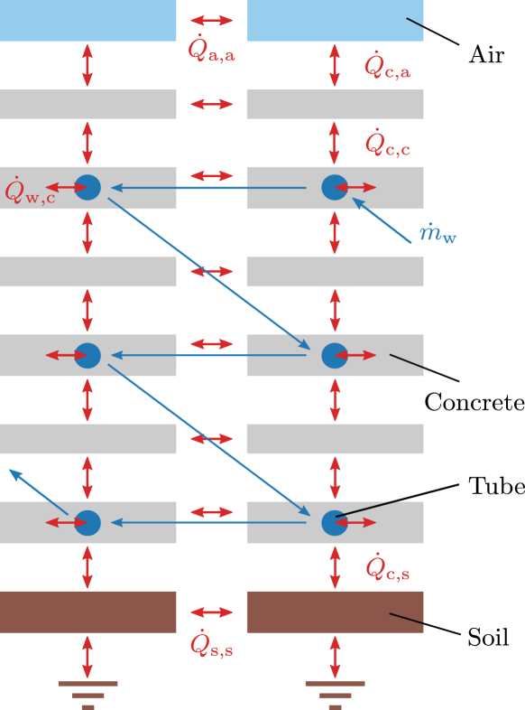
The tube inside the cage is modeled by a number of fluid-filled volumes that exchange media and heat with neighboring volumes. The temperature $T_{\mathrm{cs,w}}$ within such a volume is calculated as

$$\begin{split}\dot{T}_{\mathrm{cs,w}}(t)={}&(\rho_{\mathrm{w}}V_{\mathrm{cs,w}})^{-1}\Bigl{(}\dot{m}_{\mathrm{cs,t}}(t)(T_{\mathrm{cs,w,pre}}(t)\\ &-T_{\mathrm{cs,w}}(t))-c_{\mathrm{w}}^{-1}\dot{Q}_{\mathrm{cs,w,c}}(t)\Bigr{)}\end{split}$$ (1)

$$\begin{split}\dot{m}_{\mathrm{cs,t}}(t)={}&n_{\mathrm{cs}}^{-1}\Big{(}\dot{m}_{\mathrm{cs}}(t)\\ &+r_{\mathrm{lt,ht}}(1.0-r_{\mathrm{lts,cs}}(t))\dot{m}_{\mathrm{rt}}(t)\Big{)}\end{split}$$ (2)

$$\dot{Q}_{\mathrm{cs,w,c}}(t)={} \alpha_{\mathrm{cs,w,c}}A_{\mathrm{cs,w,c}}(T_{\mathrm{cs,w}}(t)-T_{\mathrm{cs,c}}(t))$$ (3)

with $V_{\mathrm{cs,w}}$ the constant fluid volume and $A_{\mathrm{cs,w,c}}$ the heat exchange area between fluid and concrete (i. e., the tube surface within the volume) depending on the discretization, $\alpha_{\mathrm{cs,w,c}}$ a constant heat transfer coefficient and $T_{\mathrm{cs,c}}$ the temperature of the surrounding concrete. For the volume at the inlet of the CS, $T_{\mathrm{cs,w,pre}}$ results from the mixing of the RT outlet temperature $T_{\mathrm{rt}}$ and the LTS outlet temperature $T_{\mathrm{lts}}$ according to their mass flow ratios, for the upcoming volumes it is the temperature of the preceding volume.

Concrete within the cage is modeled by a number of solid volumes that exchange only heat with neighboring volumes. The temperature within a concrete volume $T_{\mathrm{cs,c}}$ is calculated as

$$\dot{T}_{\mathrm{cs,c}}(t)={} (\rho_{\mathrm{c}}V_{\mathrm{cs,c}}c_{\mathrm{c}})^{-1}\left(\dot{Q}_{\mathrm{cs,c,s}}(t)+\dot{Q}_{\mathrm{cs,c,a}}(t)\right.$$ (4)

$$\left.+\dot{Q}_{\mathrm{cs,w,c}}(t)+\textstyle\sum_{i}\dot{Q}_{\mathrm{cs,c,c},i}(t)\right)$$

where $\dot{Q}_{\mathrm{cs,c,s}}$ is the heat flowing from the center of the volume towards a neighboring soil volume (if existing), $\dot{Q}_{\mathrm{cs,c,a}}$ towards a neighboring air volume (if existing) and $\dot{Q}_{\mathrm{cs,c,c},i}$ towards the $i$th neighboring concrete volume. Accordingly, the temperature $T_{\mathrm{cs,s}}$ within a soil volume is calculated as

$$\dot{T}_{\mathrm{cs,s}}(t)=\frac{\dot{Q}_{\mathrm{cs,s,c}}(t)+\textstyle\sum_{i}\dot{Q}_{\mathrm{cs,s,s},i}(t)}{\rho_{\mathrm{s}}V_{\mathrm{cs,s}}c_{\mathrm{s}}}$$ (5)

and the temperature $T_{\mathrm{cs,a}}$ within an air volume as

$$\dot{T}_{\mathrm{cs,a}}(t)=\frac{\dot{Q}_{\mathrm{cs,a,c}}(t)+\textstyle\sum_{i}\dot{Q}_{\mathrm{a,a},i}(t)}{\rho_{\mathrm{a}}V_{\mathrm{cs,a}}c_{\mathrm{a}}}.$$ (6)

Heat exchange between solid volumes is modeled depending on the adjoining heat exchange areas of volumes, the distance from the volume center to these areas and the thermal conductivity of the contained material, so that the current heat flow $\dot{Q}_{\mathrm{x,y}}$ between two solid volumes with temperatures $T_{\mathrm{x}}$ and $T_{\mathrm{y}}$ is given by

$$\dot{Q}_{\mathrm{x,y}}(t)=A\lambda_{x}\lambda_{y}\frac{T_{\mathrm{x}}(t)-T_{\mathrm{y}}(t)}{\Delta_{x}\lambda_{y}+\Delta_{y}\lambda_{x}},$$ (7)

with $\lambda_{\mathrm{\{x,y\}}}$ the thermal conductivities, $A$ the area of the adjoining surfaces and $\Delta_{\mathrm{\{x,y\}}}$ the distances of the center from the adjoining surface of a volume.

While for the MPC model the discretization is deducted only along the height and width of the cage as shown shown in Figure 3, additional discretization using $n_{l}=5$ volumes along the length of the cage has been applied for the simulation model. Furthermore, within the MPC model, the fraction of the mass flow from the RT through the CS is introduced as an individual control variable $\dot{m}_{\mathrm{rt,cs}}$ such that (2) is replaced by

$$\dot{m}_{\mathrm{cs,t}}(t)=n_{\mathrm{cs}}^{-1}(\dot{m}_{\mathrm{cs}}(t)+\dot{m}_{\mathrm{rt,cs}}(t))$$ (8)

to reduce nonlinearity of the MPC model.

3.2 Storages

Both the LTS and HTS are modeled by a number of water-filled balance volumes. In both $f_{\mathrm{sim}}$ and $f_{\mathrm{mpc}}$, a discretization along the height of the storages using $n_{\mathrm{lts}}=n_{\mathrm{hts}}=5$ volumes is deducted to depict temperature stratifications inside each storage, while the mass exchange and corresponding flow directions between the several volumes depend on the current mass flows at the storages in- and outlets, cf. Streckiene et al. (2011).

For the simulation model, the energy balance that determines the temperature $T_{\mathrm{lts},1}$ of the LTS bottom volume is formulated as

$$\dot{T}_{\mathrm{lts},1}(t)={} (\rho_{\mathrm{w}}V_{\mathrm{lts}})^{-1}\Bigl{(}\dot{m}_{\mathrm{cs}}(t)T_{\mathrm{cs,w},-1}(t)$$ (9)

$$+r_{\mathrm{lt,ht}}(t)r_{\mathrm{lts,cs}}(t)\dot{m}_{\mathrm{rt}}(t)T_{\mathrm{rt},-1}(t)$$

$$+b_{\mathrm{hp}}\dot{m}_{\mathrm{hp,lt}}(t)T_{\mathrm{hp,lt}}(t)$$

$$-\dot{m}_{\mathrm{l,lt}}(t)T_{\mathrm{lts},1}(t)$$

$$+\dot{m}_{\mathrm{lts,+}}(t)T_{\mathrm{lts},2}(t)$$

$$-\dot{m}_{\mathrm{lts,-}}(t)T_{\mathrm{lts},1}(t)\Bigr{)}$$

where $V_{\mathrm{lts}}$ is a constant fluid volume of the LTS, $T_{\mathrm{cs,w},-1}$ the CS outlet water temperature, $T_{\mathrm{rt},-1}$ the RT outlet temperature, $\dot{m}_{\mathrm{hp,lt}}$ the mass flow rate and $T_{\mathrm{hp,lt}}$ the outlet temperature of the LT side of the HP and $\dot{m}_{\mathrm{l,lt}}$ the LT load mass flow. The mass flows $\dot{m}_{\mathrm{lts},+}$ and $\dot{m}_{\mathrm{lts},-}$ from and towards the neighboring storage volume, respectively, are determined by the mass balances

$$\begin{split}\dot{m}_{\mathrm{lts},+}(t)={}&\max(0,\,\dot{m}_{\mathrm{l,lt}}(t)-\dot{m}_{\mathrm{cs}}(t)\\ &-r_{\mathrm{lt,ht}}(t)r_{\mathrm{lts,cs}}(t)\dot{m}_{\mathrm{rt}}(t)\\ &-b_{\mathrm{hp}}\dot{m}_{\mathrm{hp,lt}}(t))\end{split}$$ (10)

$$\begin{split}\dot{m}_{\mathrm{lts},-}(t)={}&\max(0,\,\dot{m}_{\mathrm{cs}}(t)+b_{\mathrm{hp}}\dot{m}_{\mathrm{hp,lt}}(t)\\ &+r_{\mathrm{lt,ht}}(t)r_{\mathrm{lts,cs}}(t)\dot{m}_{\mathrm{rt}}(t)\\ &-\dot{m}_{\mathrm{l,lt}}(t))\end{split}$$ (11)

and are valid for all volumes within the LTS, so it is not necessary to compute these balances for each discrete volume individually.

The discontinuities introduced to $f_{\mathrm{sim}}$ by 10 and 11 must be avoided within $f_{\mathrm{mpc}}$ to preserve differentiability. One possible way to achieve this would be to use only one volume per storage, however, not representing storage stratification at all results in insufficient information for the MPC on the current storage state and can therefore lead to severe performance losses regarding both optimality as well as constraint satisfaction.

Therefore, it should be preferred to introduce multiple volumes per storage and suitable, smooth approximations for the mass flows between those. According to the method presented by Sawant et al. (2019) and introducing a separate control variable $\dot{m}_{\mathrm{rt,lts}}$ for the fraction of the mass flow from the RT through the LTS to reduce model nonlinearity, Eq. (9) is reformulated for use within $f_{\mathrm{mpc}}$ as

$$\begin{split}\dot{m}_{\mathrm{lts,s}}(t)={}&\dot{m}_{\mathrm{rt,lts}}(t)+\dot{m}_{\mathrm{cs}}(t)\\ &+b_{\mathrm{hp}}\dot{m}_{\mathrm{hp,lt}}(t)-\dot{m}_{\mathrm{l,lt}}(t)\end{split}$$ (12)

$$\dot{m}_{\mathrm{lts,\bar{s}}}(t)={} \sqrt{\dot{m}_{\mathrm{lts,s}}^{2}(t)+\epsilon\,}$$ (13)

$$\begin{split}\dot{T}_{\mathrm{lts},1}(t)={}&(\rho_{\mathrm{w}}V_{\mathrm{lts}})^{-1}\biggl{(}\dot{m}_{\mathrm{cs}}(t)T_{\mathrm{cs,w},-1}(t)\\ &+\dot{m}_{\mathrm{rt,lts}}(t)T_{\mathrm{rt},-1}(t)\\ &+b_{\mathrm{hp}}\dot{m}_{\mathrm{hp,lt}}(t)T_{\mathrm{hp,lt}}(t)\\ &-\dot{m}_{\mathrm{l,lt}}(t)T_{\mathrm{lts},1}(t)\\ &-\Bigl{(}\dot{m}_{\mathrm{lts,s}}(t)(T_{\mathrm{lts},1}(t)+T_{\mathrm{lts},2}(t))/2\\ &+\dot{m}_{\mathrm{lts,\bar{s}}}(t)(T_{\mathrm{lts},1}(t)-T_{\mathrm{lts},2}(t))/2\Bigr{)}\biggr{)}.\end{split}$$ (14)

Though the approximation of the absolute value in (13) is better the smaller $\epsilon$ is chosen, smaller values for $\epsilon$ increase the nonlinearity introduced to the model, so that $\epsilon$ must be considered as a tuning parameter and chosen based on the actual quantities of the mass flows. Within this study, $\epsilon=0.5$ is used.

The HTS is modeled analogously to the LTS, however $T_{\mathrm{hts},1}$ marks the temperature of the top volume of the HTS. The HR is installed in the top and can therefore be used to directly increase $T_{\mathrm{hts},1}$. Also, the mass flow from the RT to the HTS is introduced as an individual control $\dot{m}_{\mathrm{rt,hts}}$ in $f_{\mathrm{mpc}}$, accordingly to $\dot{m}_{\mathrm{rt,lts}}$ for the LTS.

3.3 Heat pump

For modeling the HP, we assume that its internal controller realizes a constant temperature difference of $\Delta T_{\mathrm{hp}}=4\,\mathrm{K}$ between inlet and outlet on both the LT and HT side of the HP as in

$$T_{\mathrm{hp,ht}}(t) =T_{\mathrm{hts},n_{\mathrm{hts}}}(t)+\Delta T_{\mathrm{hp}},$$ (15)

$$T_{\mathrm{hp,lt}}(t) =T_{\mathrm{lts},n_{\mathrm{lts}}}(t)-\Delta T_{\mathrm{hp}}.$$ (16)

The COP is calculated from the Carnot COP for the machine and a degree of efficiency factor $\eta_{\mathrm{hp}}=0.52$ as in

$$\mathrm{COP}_{\mathrm{hp}}(t)=\eta_{\mathrm{hp}}\frac{T_{\mathrm{hp,ht}}(t)}{T_{\mathrm{hp,ht}}(t)-T_{\mathrm{hp,lt}}(t)}.$$ (17)

Using $\mathrm{COP}_{\mathrm{hp}}$ and the electrical power $P_{\mathrm{hp,el}}$ of the machine, the heating power $\dot{Q}_{\mathrm{hp,ht}}$ and cooling power $\dot{Q}_{\mathrm{hp,lt}}$ under current operation conditions can be computed as

$$\dot{Q}_{\mathrm{hp,ht}}(t) =\mathrm{COP}_{\mathrm{hp}}(t)P_{\mathrm{hp,el}}(t),$$ (18)

$$\dot{Q}_{\mathrm{hp,lt}}(t) =\dot{Q}_{\mathrm{hp,ht}}(t)-P_{\mathrm{hp,el}}(t).$$ (19)

Finally, the current mass flow on the LT and HT side of the machine can be calculated as

$$\dot{m}_{\mathrm{hp,lt}}(t) =\frac{\dot{Q}_{\mathrm{hp,lt}}(t)}{c_{\mathrm{w}}(T_{\mathrm{lts},n_{\mathrm{lts}}}(t)-T_{\mathrm{hp,lt}}(t))},$$ (20)

$$\dot{m}_{\mathrm{hp,ht}}(t) =\frac{\dot{Q}_{\mathrm{hp,ht}}(t)}{c_{\mathrm{w}}(T_{\mathrm{hp,ht}}(t)-T_{\mathrm{hts},n_{\mathrm{hts}}}(t))}.$$ (21)

3.3.1 Recooling tower

The RT is modeled by a number of fluid volumes that exchange heat with their environment depending on ambient temperature $T_{\mathrm{amb}}$ and current RT operation level $r_{\mathrm{rt,op}}$. Since the RT is designed as an air-water cross-flow heat exchanger, air mass flows are assumed to be high and resulting air temperature differences small. Following this assumption, no further air balance volume discretization is conducted. For simplicity, $r_{\mathrm{tr,op}}$ is modeled to directly influence the current heat exchange of the RT, so that the temperature $T_{\mathrm{rt}}$ within a balance volume is calculated as

$$\dot{T}_{\mathrm{rt}}(t)={} \frac{\dot{m}_{\mathrm{rt}}(t)(T_{\mathrm{rt,pre}}(t)-T_{\mathrm{rt}}(t))-\frac{\dot{Q}_{\mathrm{rt}}(t)}{c_{\mathrm{w}}}}{\rho_{\mathrm{w}}V_{\mathrm{rt}}}$$ (22)

$$\dot{Q}_{\mathrm{rt}}(t)={} r_{\mathrm{rt,op}}(t)\alpha_{\mathrm{rt}}A_{\mathrm{rt}}(T_{\mathrm{rt}}(t)-T_{\mathrm{amb}}(t))$$ (23)

with $V_{\mathrm{rt}}$ the constant fluid volume and $A_{\mathrm{rt}}$ the heat exchange area between fluid and outside environment depending on the discretization. For the volume at the inlet of the RT, $T_{\mathrm{rt,pre}}$ results from the mixing of the outlet temperatures of CS, LTS and HTS according to their mass flow ratios, for the upcoming volumes it is the temperature of the preceding volume.

While for the MPC model the RT is modeled using a single volume, the RT is discretized into $n_{\mathrm{rt}}=5$ volumes for the simulation model.

3.4 Modeling of thermal loads of the building

Cooling loads $\dot{Q}_{\mathrm{l,lt}}$ are covered from the LTS and heating loads $\dot{Q}_{\mathrm{l,ht}}$ from the HTS. In the following, we assume that an internal, low-level controller realizes a constant temperature difference $\Delta T_{\mathrm{l}}$ by supply flow addition in the heating and cooling circuits, while setting the mass flows in the distribution circuits to meet demands. The return temperatures and mass flows entering and leaving the storages are then given by

$$T_{\mathrm{l,lt}}(t)={} T_{\mathrm{lts},1}(t)+\Delta T_{\mathrm{l}},$$ (24)

$$\dot{m}_{\mathrm{l,lt}}(t)={} \left(c_{\mathrm{w}}\Delta T_{\mathrm{l}}\right)^{-1}\dot{Q}_{\mathrm{l,lt}}(t),$$ (25)

$$T_{\mathrm{l,ht}}(t)={} T_{\mathrm{hts,1}}(t)-\Delta T_{\mathrm{l}},$$ (26)

$$\dot{m}_{\mathrm{l,ht}}(t)={} \left(c_{\mathrm{w}}\Delta T_{\mathrm{l}}\right)^{-1}\dot{Q}_{\mathrm{l,ht}}(t).$$ (27)

While utilization of a detailed building model may facilitate further efficiency gains within the later control applications, this would also further increase the complexity of the model through addition of multiple states and control variables, and is therefore considered future work.

3.5 Auxiliary states

The MPC model contains the auxiliary states $C_{\dot{Q}_{\mathrm{l,lt}}}$, $C_{\dot{Q}_{\mathrm{l,ht}}}$ and $C_{T_{\mathrm{amb}}}$ used for compensation of deviations between forecasted and measured time-varying parameters to increase performance of the MPC. Those are determined by solving an MHE problem in between two subsequent MPC steps. Exemplary, the auxiliary state for $T_{\mathrm{amb}}$ reads as

$$\dot{C}_{T_{\mathrm{amb}}}(t)=-(\tau_{C}^{-1}C_{T_{\mathrm{amb}}}(t))$$ (28)

with $\tau_{C}$ a time constant which allows for modeling a decaying influence of the current deviation with increasing time. With this and $T_{\mathrm{amb,fc}}$ the raw forecast inputs, $T_{\mathrm{amb}}$ then enters $f_{\mathrm{mpc}}$ as

$$T_{\mathrm{amb}}(t)=T_{\mathrm{amb,fc}}(t)+C_{T_{\mathrm{amb}}}(t).$$ (29)

4 Development of a conventional control strategy

In the following, an elaborate Conventional Control (CC) strategy for the system is described, which has been developed and improved iteratively using the presented simulation model. A schematic depiction of the CC loop is given in Figure 4.

Figure 4: Schematic depiction of the CC loop.

4.1 General controller design principles

The CC strategy aims at covering heating and cooling demands in a reliable and simultaneously energy efficient manner, realized through a sophisticated storage management approach. Since requirements regarding storage management differ between seasons, separate operation modes have been developed for summer and winter operation, which are described in more detail in the upcoming sections. Transition between summer and winter mode is carried out at fixed time points during the year.

Activation of devices is mainly realized using set-point-based control and switching hystereses depending on current temperatures of LTS, HTS, RT and CS. Mass flows $\dot{m}_{\mathrm{rt}}$, $\dot{m}_{\mathrm{cs}}$ and ratios $r_{\mathrm{lts,cs}}$, $r_{\mathrm{rt,op}}$ are determined using PI-controllers depending on specified temperature differences between inlets and outlet of the several components. Despite technically possible, $r_{\mathrm{lt,ht}}$ is not chosen on a continuous scale within the CC but always fully switched depending on whether the HP is currently mainly used for covering of cooling or heating demands.

4.2 Operation in summer mode

Summer mode is especially focused on covering cooling loads with irregularly occurring heating demands. For this, the following hierarchy for activation of cooling devices for decreasing LTS temperature is defined: 1) free cooling via the RT, 2) storing energy from the cooling loads in the CS, and 3) cooling via the HP.

In times of spare cooling capacity, the LTS and the CS are cooled down using free cooling via the RT. In case their temperatures have exceeded a certain threshold value, also the HP is used to pro-actively cool down these storages in order to generate cooling energy under more favorable conditions and store it for later usage. If the HTS temperature increases too much during HP operation, the HTS is cooled down via the RT. Occurring heating loads are covered utilizing the HP.

In case the HP is active, the current driving power $P_{\mathrm{hp,el}}$ for the HP is modulated in order to cover the maximum of a) the current heating load and b) the current cooling load that cannot be covered using RT and CS.

4.3 Operation in winter mode

Winter mode is especially focused on covering heating loads while accounting for the permanently occurring cooling demands caused by the running server computers, but also for irregularly occurring cooling demands arising, e. g., in case of high solar irradiation on the building. Free cooling via the RT is avoided and storing the energy from cooling loads in the CS is preferred to facilitate later usage for covering of heating demands via the HP.

In case the heating demands exceed the cooling demands in winter mode, RT and CS are utilized to increase the LTS temperature to prevent undercooling. In case the LT side of the system cannot provide enough energy for operation of the HP, the HRs are utilized to cover remaining loads.

4.4 Setup and implementation

Simulation model $f_{\mathrm{sim}}$ and the CC strategy are implemented in Modelica and simulated using Dymola 2019 with DASSL integrator, which directly facilitates a simulation of the CC strategy.

5 Development of a model-predictive control strategy

In this section, the MPC strategy is presented by first introducing the Optimal Control Problem (OCP) formulated for the controller and the utilized solution strategy and software implementation, followed by the formulation and implementation of the MHE problem used for compensation of model mismatch and forecast deviations. A schematic depiction of the MPC loop is given in Figure 5.

Figure 5: Schematic depiction of the MPC loop.

5.1 OCP formulation

Within the OCP, all boundaries on non-auxiliary system states, which are the temperature constraints for the several components, are formulated as soft constraints to prevent infeasibility of the OCP in case of state constraint violations, cf. Rawlings et al. (2017). For this, we introduce a vector of $n_{s}=33$ slack variables $s$.

With continuous controls $u^{\top}=[\dot{m}_{\mathrm{rt,hts}}~{}\allowbreak\dot{m}_{\mathrm{rt,lts}}~{}\allowbreak\dot{m}_{\mathrm{rt,cs}}~{}\allowbreak\dot{m}_{\mathrm{cs}}~{}\allowbreak r_{\mathrm{rt,op}}~{}\allowbreak P_{\mathrm{hr}}~{}\allowbreak P_{\mathrm{hp,el}}]$ and time-varying parameters $c^{\top}=[T_{\mathrm{amb,fc}}~{}\allowbreak\dot{Q}_{\mathrm{l,lt,fc}}~{}\allowbreak\dot{Q}_{\mathrm{l,ht,fc}}]$, the Mixed-Integer Optimal Control Problem (MIOCP) reads as

$$\hskip 0.0pt\mkern-35.0mu\begin{aligned} \underset{{\begin{subarray}{c}x(\cdot),u(\cdot),\\ b_{\mathrm{hp}}(\cdot),s(\cdot)\end{subarray}}}{\mathrm{min}}&\hskip 5.69046pt\int_{t_{0}}^{t_{\text{f}}}\left(s(t)^{\top}W_{s}s(t)+w_{s}^{\top}s(t)\right)\,\text{d}t\\ &\hskip 5.69046pt+\int_{t_{0}}^{t_{\text{f}}}w_{u}^{\top}u(t)\,\text{d}t\\ \end{aligned}$$ (30a)

$$\mathrm{s.\,t.} \hskip 2.84544pt\text{for }t\in[t_{0},t_{\mathrm{f}}]:$$

$$\hskip 2.84544pt\dot{x}(t)=f_{\mathrm{mpc}}(x(t),u(t),b_{\mathrm{hp}}(t),c(t)),$$ (30b)

$$\hskip 2.84544pt0\leq\sum\dot{m}_{\mathrm{rt,\{hts,lts,cs\}}}(t)\leq\dot{m}_{\mathrm{rt,max}},$$ (30c)

$$\hskip 2.84544pt0\leq\dot{m}_{\mathrm{rt,cs}}(t)+\dot{m}_{\mathrm{cs}}(t)\leq\dot{m}_{\mathrm{cs,max}},$$ (30d)

$$\hskip 2.84544ptT_{\mathrm{lb}}-s(t)\leq Zx(t)\leq T_{\mathrm{ub}}+s(t),$$ (30e)

$$\hskip 2.84544ptu_{\mathrm{lb}}\leq u(t)\leq u_{\mathrm{ub}},$$ (30f)

$$\hskip 2.84544ptb_{\mathrm{hp}}(t)\in\{0,1\},$$ (30g)

$$\hskip 2.84544pts(t)\geq 0,$$ (30h)

$$\hskip 2.84544ptx(t_{0})=x_{0}.$$ (30i)

The objective of the MIOCP given in (30a) is a Lagrange-type objective and contains the sum of squares of the slack variables, the sum of the slack variables and the sum of the continuous controls, weighted by appropriate diagonal weighting matrix $W_{\mathrm{s}}\in\mathbb{R}^{n_{s}\times n_{s}}$ and vectors $w_{\mathrm{s}}\in\mathbb{R}^{n_{s}}$ and $w_{\mathrm{u}}\in\mathbb{R}^{n_{u}}$, respectively. The dynamics of the system are given in (30b). Equations 30c and 30d ensure that the maximum mass flows through RT and CS are not exceeded. With $Z$ a selection matrix that selects the constrained temperatures from $x$, the soft constraints for the state boundaries are given in (30e), while the boundaries on the continuous controls are given as hard constraints in (30f). Finally, the binary constraint is given in (30g), positivity of the slack variables is ensured by (30h) and the initial state constraint is given in (30i).

5.2 OCP setup and implementation

For solving OCPs, utilization of direct methods, especially direct multiple shooting (Bock and Plitt, 1984) or direct collocation (Tsang et al., 1975), is favorable, cf. Sager (2009); Binder et al. (2001). For implementation and solution of (30), a control horizon of $t_{\mathrm{f}}=24\,\mathrm{h}$ has been chosen and discretized into $N=29$ control intervals, whereof the first 6 intervals are of length $\Delta t_{\mathrm{s}}=10\,\mathrm{min}$ and the remaining 23 intervals of length $\Delta t_{\mathrm{l}}=1\,\mathrm{h}$, using direct collocation with Lagrange polynomials with Radau collocation points.

For solution of the resulting MINLP on MPC suitable time scales, application of general MINLP solvers is usually not favorable. Therefore, the decomposition approach by Sager (2009) is applied, where the solution of the original MINLP is approximated by solving first a relaxed version of the MINLP, which is a Non-Linear Program (NLP), then obtaining an integer trajectory for the discrete controls by application of either Sum-Up-Rounding (SUR) (Sager, 2009) or Combinatorial Integral Approximation (CIA) (Sager et al., 2011), and afterwards solving the NLP again with binary controls fixed according to the solution of the integer approximation step. In the literature, several successful applications of this approach can be found (Kirches, 2011; Ebrahim et al., 2018; Bürger et al., 2018a).

The NLP is implemented using the dynamic optimization framework CasADi (Andersson et al., 2018) in Python. For solution of the arising NLPs, Ipopt (Wächter and Biegler, 2006) with linear solver MA57 (HSL, 2018) is used. For solution of the integer approximation problem, the binary approximation package pycombina is applied, which is presented in Bürger et al. (2018b).

The controls for the system obtained by solution of the MINLP for the first 10 min of the control horizon are applied to the simulation model $f_{\mathrm{sim}}$ implemented in Modelica to accept external control inputs via the Python interface of Dymola.

Figure 6: Heating demands $\dot{Q}_{\mathrm{l,lt}}$, cooling demands $\dot{Q}_{\mathrm{l,ht}}$ and ambient temperatures $T_{\mathrm{amb}}$ assumed within this study. In the left hand side plots, suffix “fc” indicates forecasts used for the MPC and suffix “m” indicates corresponding measured values used for simulation. The hatched blue area marks the constant cooling demand induced by the server computers. The right hand side plots are violin plots showing the distribution of the deviations from forecasts to measurements.

5.3 MHE formulation

The MHE problem for estimation of the current system state and compensation of the current forecast deviations based on the previous $M=4$ measurements reads as

$$\hskip 0.0pt\mkern-35.0mu\begin{aligned} \underset{x(\cdot),w(\cdot)}{\mathrm{min}}&\hskip 5.69046pt\sum_{k=0}^{M}\|y(x_{k},u_{k},b_{\mathrm{hp},k},c_{k})-x_{k}\|_{W^{-1}}^{2}\\ &\hskip 5.69046pt+\sum_{k=0}^{M}\|w_{k}\|_{Q^{-1}}^{2}+\|x_{0}-\hat{x}\|_{P^{-1}}^{2}\\ \end{aligned}$$ (31a)

$$\mathrm{s.\,t.} \hskip 2.84544pt\text{for }k=0,\dots,M-1:$$

$$\hskip 5.69046ptx_{k+1}=\bar{f}_{\mathrm{mpc}}(x_{k},u_{k},b_{\mathrm{hp},k},c_{k},w_{k})$$ (31b)

with $y$ the measurement function and $W$ the covariance matrix of the measurements, $w$ an additive process noise with covariance matrix $Q$ acting on the system state, $\|x_{0}-\hat{x}\|_{P^{-1}}^{2}$ the arrival cost with covariance matrix $P$, and $\bar{f}_{\mathrm{mpc}}$ the solution of the MPC model for a discrete time step.

More detailed information on MHE and interpretation of the arrival cost can be found in, e. g., Kühl et al. (2011) and Kraus et al. (2013).

5.4 MHE setup and implementation

Similar to the OCP, the MHE problem is implemented using direct collocation and the arising NLPs are solved using Ipopt and MA57. An application of the decomposition approach is not necessary, as the MHE problem contains no discrete optimization variables. Arrival cost updates are conducted using a smoothened Extended Kalman Filter (EKF), cf. Girrbach et al. (2018).

The resulting measurements after simulating the first 10 min of the horizon in Dymola are passed as measurements to the MHE. The estimated system states resulting from solution of the MHE problem are then used for initialization of the subsequent MPC step. By repeating this procedure, a simulation of the MPC strategy is carried out.

6 Comparison of controller performances

In the following, the controller performances are compared on an annual simulation for each controller. All computations are conducted on a Fujitsu P920 Desktop PC with an Intel Core i5-4570 3.20 GHz CPU and 16 GB RAM running Debian 9, using Python 3.5, gcc 6.3, Dymola 2019, CasADi 3.4.5 and pycombina 0.2.

6.1 Scenario of the simulation study

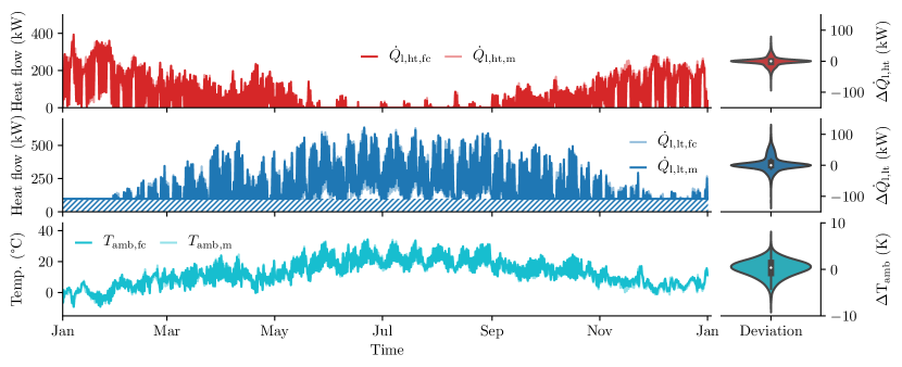
The forecasted and measured thermal loads $\dot{Q}_{\mathrm{l,ht},\{\mathrm{fc,m}\}}$ and $\dot{Q}_{\mathrm{l,lt},\{\mathrm{fc,m}\}}$ of the building assumed within this study are calculated using a dynamic building simulation in accordance to VDI 2078 based on forecasts and measured weather data provided by City of Karlsruhe (2017). These are depicted in Figure 6 next to the forecasted and measured ambient temperature $T_{\mathrm{amb},\{\mathrm{fc,m}\}}$.

For realistic initialization of the system states, their initial values have been chosen based on the final states obtained from preliminary simulations.

6.2 Comparison of simulation results

Figure 7: Simulated temperatures within HTS, LTS and CS throughout the year obtained by MPC and CC. The upper plots show the temperatures $T_{\mathrm{hts,1}}$ at the top and $T_{\mathrm{hts,5}}$ at the bottom of the HTS, the dashed black lines indicate the temperature constraints for $T_{\mathrm{hts,1}}$. The middle plots show the temperatures $T_{\mathrm{lts,1}}$ at the bottom and $T_{\mathrm{lts,5}}$ at the top of the LTS, the dashed black lines indicate the temperature constraints for $T_{\mathrm{lts,1}}$. The lower plots show the water temperatures $T_{\mathrm{cs,w,1}}$ at the inlet and $T_{\mathrm{cs,w,5}}$ at the outlet of the CS and the dashed black lines denote their constraints.

Figure 8: Detailed view on system operation using MPC (left) and CC (right) in January.

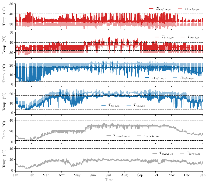
An overview of the results of the simulation study is given in Figure 7 by the temperatures of the HTS, LTS and CS throughout the year for both MPC and CC. The plot reveals substantially different behaviors of the controllers, which is discussed in more detail in the following.

6.2.1 LTS and HTS management

Figure 7 shows that the CC aims to achieve a certain margin of the storage temperatures from their boundary values. This is necessary for the controller to stay reactive in case of altering loads. Therefore, it takes action once a temperature value moves close towards a boundary and drives the temperature value towards the opposite direction.

For the MPC however, it can be observed that the controller runs the storage on temperatures which are very close to their respected boundaries. Explicitly, the MPC tries to always run the LTS at the upper temperature boundary and the HTS at the lower temperature boundary. This increases the efficiency of the HP, and consequently, decreases its electrical power consumption.

Figure 9: Detailed view on system operation using MPC (left) and CC (right) in May.

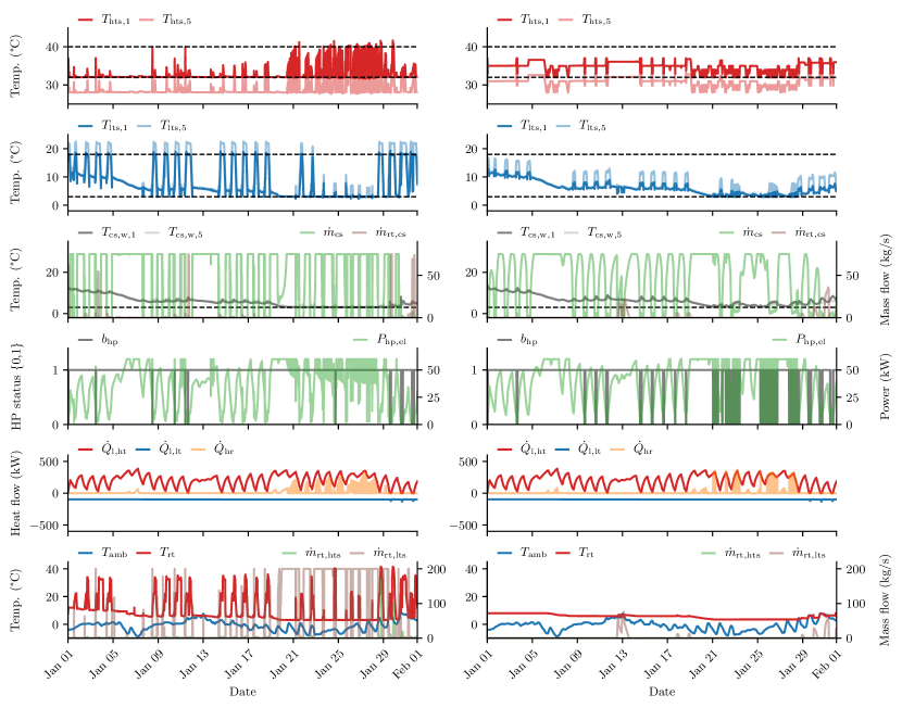
A more detailed depiction of this behavior can be found in Figure 8, which depicts the trajectories of states and controls in January. Here, the LTS acts as a heat source for the HP, and it can be observed how the MPC favors HP efficiency by increasing the temperature of the LTS periodically in times of low heating load while keeping the HTS temperature at its lower boundary. Consistently, it can be seen that the electric power $P_{\mathrm{hp,el}}$ consumed by the HP is often lower for the MPC than for the CC.

Operation of the storages this close to their respected boundary temperatures is only possible due to the incorporation of (corrected) forecasts in the MPC strategy and its knowledge of the system behavior through the included model $f_{\mathrm{mpc}}$. This is a clear advantage of the MPC over the CC, however, coming at the price of an increased complexity of controller design and implementation.

6.2.2 Concrete slab utilization

Figure 10: Detailed view on system operation using MPC (left) and CC (right) in August.

The winter mode of the CC strategy, which is designed for times dominated by heating loads, utilizes the CS to increase the temperature of the LTS, and with this, as a heat source for the HP covering the occurring heating loads. During such load scenarios, the MPC utilizes the CS similarly to the CC, as shown by the CS temperatures in Figure 7 and by the CS temperatures, pump operation and HP operation in Figure 8.

In times dominated by cooling loads though, the strategies of the controllers differ. Here, the summer mode of the CC utilizes the CS to provide cooling power for reducing the temperature of the LTS, i. e., to store energy from the LTS, and is regenerated in times of low ambient temperatures using the RT or, in rare cases, the HP.

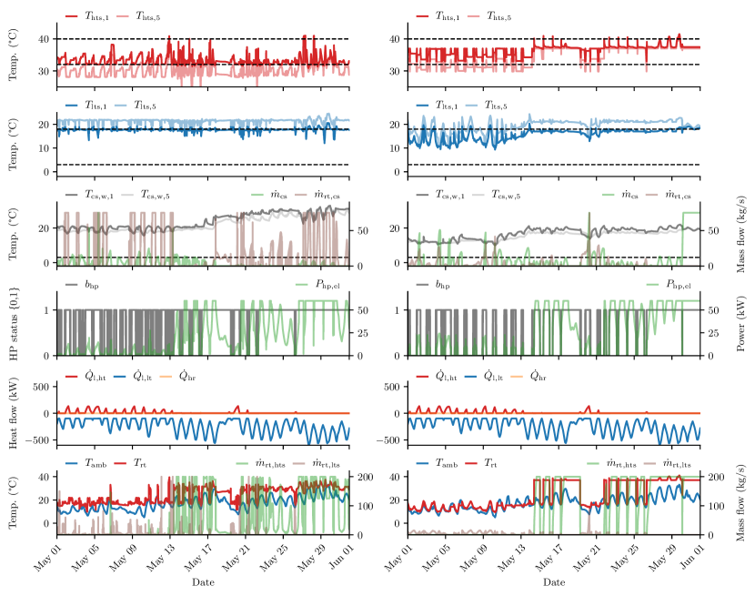
The MPC however utilizes the CS to store energy also from the HTS. More insight into the reason behind this can be found in Figure 9, which depicts the trajectories of states and controls in May. While it is shown that in the first half of the month the MPC uses the CS similarly to the CC as a cold source for the LTS, in the second half of the month the MPC realizes mass flows from the HTS to the RT and from the CS to the RT at the same time, which results in the CS being used as a recooling device for the HP. Due to the lower recooling temperature supported to the HTS in comparison of using only the RT individually, the operation efficiency of the HP increases.

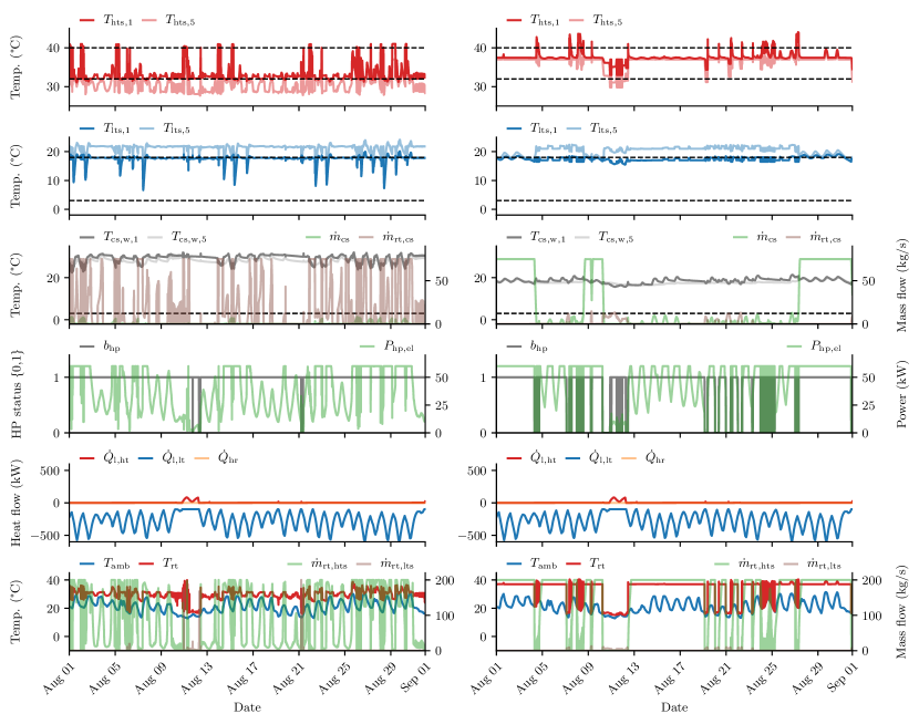
The energy stored in the CS this way can then be emitted to the ambient via the RT during times of lower ambient temperature. A higher temperature difference between CS and ambient can also be achieve easier now as if the CS was used to merely cool down the LTS which operates at a much lower maximum temperature than the HTS. Further, this results in a higher utilization of the CS within the MPC when compared to the CC, which can be observed in Figure 10, which depicts the trajectories of states and controls in August.

This utilization of the CS for recooling of the HP, which turns out to be an efficient and favorable operation mode, was identified autonomously by the MPC but not during the design phase of the CC, which shows the advantages of MPC for flexible identification of situation-dependent and non-intuitive operation modes.

6.2.3 Constraint satisfaction

Figure 11: Total duration and severity of storage temperature constraint violations over the whole simulation time.

Figure 7 already indicates that for the relevant storage temperatures $T_{\mathrm{hts,1}}$ and $T_{\mathrm{lts,1}}$ as well as for the temperatures of the CS, both controllers achieve a high quality of constraint satisfaction. A more detailed analysis on the duration and levels of constraint violations throughout the year is shown in Figure 11.

The plot shows the total duration and severity of the differences between these storage temperatures and their upper and lower boundaries over the whole simulation time. For both storage temperatures, their respective boundaries are violated by more than 0.5 K in less than 572 h throughout the year, which corresponds to less than 7 % of the simulated time.

For the CC, one can observe that the lower temperature boundaries are never violated. This is due to the implementation of the CC, which does not operate on a fixed time grid and directly stops HP operation in the event of too low LTS temperatures and activates the HRs in the event of too low HTS temperatures.

The MPC, however, operates on a fixed time grid that allows changes of the requested operations of components only every $\Delta t_{\mathrm{s}}=10\,\mathrm{min}$. Since the MPC tends to operate the storage close to their boundary values, sudden mismatches between forecasted and occurring loads can cause violations of these boundaries. Such violations could possibly be further reduced by decreasing the MPC time step size $\Delta t_{\mathrm{s}}$, and consequently, the reaction time on occurring disturbances. However, due to the already high computation time for deduction of this MPC simulation study (cf. Section 6.3), this has not been further investigated.

While the violations of the upper temperature boundaries for the LTS are comparable for CC and MPC, the upper boundaries for the HTS tend to be violated less for the MPC than for the CC, which can be explained by the MPC generally operating the HTS at its lower boundary.

Figure 12: Integrated electrical energy consumption $E(t)=\int_{t_{0}}^{t}\bigl{(}P_{\mathrm{hp,el}}(\tau)+P_{\mathrm{hr}}(\tau)\bigr{)}\mathrm{d}\tau$ of HP and HRs for MPC and CC.

6.2.4 Energy consumption

The integrated electrical energy consumption of the HP and the HRs are shown for each controller in Figure 12. Until April, the consumptions are comparable and only slightly lower for the MPC, which can be explained by the similar behavior of both controllers until that time and the relatively small number of options for control actions to satisfy the high heating loads during these times.

After that, the relative consumption for the MPC reduces throughout the rest of the year due to the more efficient operation modes identified by the MPC during summer times. Also, the resulting higher amount of energy stored in the CS at the end of the warmer season can be used for driving the HP more efficiently in upcoming colder seasons. At the end of the year, the main electrical energy consumption is reduced by more than 18 % using MPC.

Additionally, using MPC drastically reduces the amount of power-cycles for the HP, which is switched merely 2135 times over the year, compared to 7075 power-cycles requested by the CC.

Figure 13: Durations of the runtime-critical stages of the MINLP solution process for all N = 52,560 steps. The boxes range from the 25 % to the 75 % quartile, the whiskers of the boxes extend these by 1.5 times the inter-quartile range. Values outside of this range are regarded as outliers and denoted as dots.

6.3 Runtime of critical MINLP solution steps

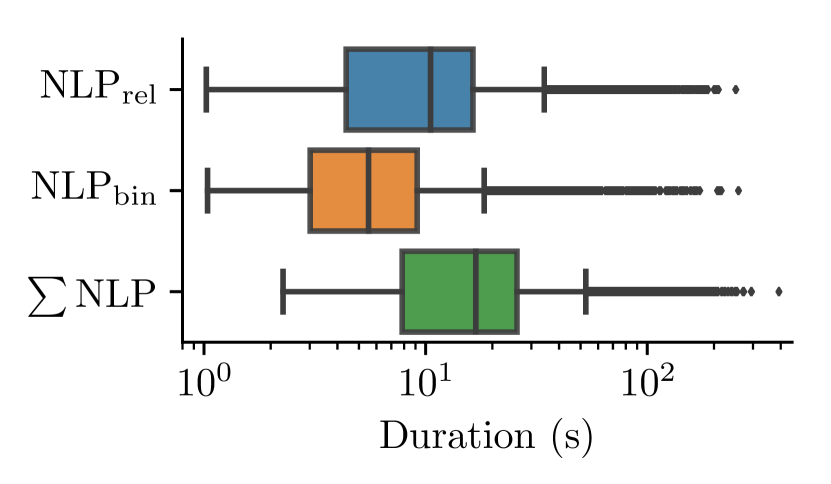
Figure 13 shows the runtimes of those MINLP solution steps with significant contribution to the overall runtime of the algorithm, which are the solutions of the NLPs described in Section 5.2. The runtime of the binary approximation step and the solution of the MHE problem within this study is always within the range of seconds and therefore negligible.

The plot shows that both the typical solution time as well as the maximum duration of both steps are below 400 s and with this far below the step size of the MPC, which renders the method generally applicable also for real-time usage on the physical system.

6.4 Significance of the MHE step

To investigate significance and impact of the MHE step on the MPC performance, several attempts have been made to run the simulation study without a dedicated state estimator and the auxiliary states described above, only utilizing simple approaches for correction of forecasts, e. g., calculation of a rolling mean on the deviations between measured and forecasted inputs. However, none of these approaches was able to sufficiently correct the forecasts, which at some point during simulation caused the MPC to fail due to severe storage temperature constraint violations. Prior to failing, constraint satisfaction was generally worse and small to medium sized violations occurred more often compared to using MHE. These findings render the MHE step significant for the overall MPC performance.

7 Conclusion

We presented a whole-year simulation study on nonlinear mixed-integer MPC for a complex thermal energy supply system and compared its performance to a conventional, set point based control strategy. We showed that MPC was able to reduce the yearly electrical energy consumption of HP and HRs by more than 18 % while providing a similar degree of constraint satisfaction. Furthermore, the MPC enabled the planner to identify previously unknown, beneficial operation modes.

Future work should consider incorporation of a detailed building model, which could facilitate further efficiency gains. Considerations on the electricity consumption of pumps could provide further potential for operation optimization. Also, through consideration of dynamic electricity prices, the system could be utilized in the context of demand response.

Conflict of interest

None.

References

-
Andersson et al. (2018)
Andersson, J. A. E., Gillis, J., Horn, G., Rawlings, J. B., Diehl, M., 2018.
CasADi: a software framework for nonlinear optimization and optimal
control. Mathematical Programming Computation.
URL https://doi.org/10.1007/s12532-018-0139-4 -
Baeten et al. (2017)
Baeten, B., Rogiers, F., Helsen, L., 2017. Reduction of heat pump induced peak
electricity use and required generation capacity through thermal energy
storage and demand response. Applied Energy 195, 184 – 195.
URL https://doi.org/10.1016/j.apenergy.2017.03.055 -
Berardi (2017)
Berardi, U., 2017. A cross-country comparison of the building energy
consumptions and their trends. Resources, Conservation and Recycling 123, 230
– 241.
URL https://doi.org/10.1016/j.resconrec.2016.03.014 -
Bianchini et al. (2019)
Bianchini, G., Casini, M., Pepe, D., Vicino, A., Zanvettor, G. G., 2019. An
integrated model predictive control approach for optimal HVAC and energy
storage operation in large-scale buildings. Applied Energy 240, 327 – 340.
URL https://doi.org/10.1016/j.apenergy.2019.01.187 -
Biegler (2010)
Biegler, L., 2010. Nonlinear Programming. Society for Industrial and Applied
Mathematics.
URL https://doi.org/10.1137/1.9780898719383 - Binder et al. (2001) Binder, T., Blank, L., Bock, H. G., Bulirsch, R., Dahmen, W., Diehl, M., Kronseder, T., Marquardt, W., Schlöder, J. P., von Stryk, O., 2001. Online Optimization of Large Scale Systems. Springer Berlin Heidelberg, Ch. Introduction to Model Based Optimization of Chemical Processes on Moving Horizons, pp. 295 – 339.
Bock and Plitt (1984)
Bock, H., Plitt, K., 1984. A multiple shooting algorithm for direct solution of
optimal control problems. IFAC Proceedings Volumes 17 (2), 1603–1608.
URL https://doi.org/10.1016/S1474-6670(17)61205-9 -
Bürger et al. (2018a)
Bürger, A., Zeile, C., Altmann-Dieses, A., Sager, S., Diehl, M.,
2018a. An algorithm for mixed-integer optimal control of solar
thermal climate systems with MPC-capable runtime. In: 2018 European Control
Conference (ECC). pp. 1379–1385.
URL https://doi.org/10.23919/ECC.2018.8550424 -
Bürger et al. (2018b)
2018b. Design, implementation and simulation of an MPC
algorithm for switched nonlinear systems under combinatorial constraints.
Last accessed May 17, 2019.
URL http://www.optimization-online.org/DB_HTML/2018/07/6713.html - City of Karlsruhe (2017) City of Karlsruhe, 2017. Dataset “Daten der Wetterstation auf der Heinrich-Hübsch-Schule” for 2017. https://transparenz.karlsruhe.de/dataset/a639453f-0c2f-4a92-a895-7353394b3e60, published under the license “Datenlizenz Deutschland - Namensnennung - Version 2.0” (https://www.govdata.de/dl-de/by-2-0), last accessed May 17, 2019.
Dainese et al. (2019)
Dainese, C., Faè, M., Gambarotta, A., Morini, M., Premoli, M., Randazzo, G.,
Rossi, M., Rovati, M., Saletti, C., 2019. Development and application of a
predictive controller to a mini district heating network fed by a biomass
boiler. Energy Procedia 159, 48 – 53, renewable Energy Integration with
Mini/Microgrid.
URL https://doi.org/10.1016/j.egypro.2018.12.016 -
Dias et al. (2018)
Dias, L. S., Pattison, R. C., Tsay, C., Baldea, M., Ierapetritou, M. G., 2018.
A simulation-based optimization framework for integrating scheduling and
model predictive control, and its application to air separation units.
Computers & Chemical Engineering 113, 139–151.
URL https://doi.org/10.1016/j.compchemeng.2018.03.009 -
Ebrahim et al. (2018)
Ebrahim, T., Subramaianan, S., Engell, S., 2018. Hybrid NMPC for switching
systems applied to a supermarket refrigeration system. In: 2018 European
Control Conference (ECC). pp. 813–818.
URL https://doi.org/10.23919/ECC.2018.8550609 -
Fischer et al. (2017)
Fischer, D., Bernhardt, J., Madani, H., Wittwer, C., 2017. Comparison of
control approaches for variable speed air source heat pumps considering time
variable electricity prices and pv. Applied Energy 204, 93 – 105.
URL https://doi.org/10.1016/j.apenergy.2017.06.110 -
Girrbach et al. (2018)
Girrbach, F., Hol, J. D., Zandbergen, R., Verschueren, R., Bellusci, G., Diehl,
M., 2018. On the effect of stabilization methods for quaternion invariants on
the uncertainty in optimization-based estimation. IFAC-PapersOnLine 51 (25),
116 – 121, 9th IFAC Symposium on Robust Control Design ROCOND 2018.
URL https://doi.org/10.1016/j.ifacol.2018.11.091 -
Hesaraki et al. (2015)
Hesaraki, A., Holmberg, S., Haghighat, F., 2015. Seasonal thermal energy
storage with heat pumps and low temperatures in building projects—a
comparative review. Renewable and Sustainable Energy Reviews 43, 1199 –
1213.
URL https://doi.org/10.1016/j.rser.2014.12.002 -
HSL (2018)
HSL, 2018. A collection of Fortran codes for large scale scientific
computation. Last accessed May 17, 2019.
URL http://www.hsl.rl.ac.uk/ -
Iovine et al. (2019)
Iovine, A., Rigaut, T., Damm, G., Santis, E. D., Benedetto, M. D. D., 2019.
Power management for a DC MicroGrid integrating renewables and storages.
Control Engineering Practice 85, 59 – 79.
URL https://doi.org/10.1016/j.conengprac.2019.01.009 -
Killian et al. (2018)
Killian, M., Zauner, M., Kozek, M., 2018. Comprehensive smart home energy
management system using mixed-integer quadratic-programming. Applied Energy
222, 662 – 672.
URL https://doi.org/10.1016/j.apenergy.2018.03.179 -
Kirches (2011)
Kirches, C., 2011. Fast Numerical Methods for Mixed-Integer Nonlinear
Model-Predictive Control. Vieweg+Teubner Verlag, Wiesbaden.
URL https://doi.org/10.1007/978-3-8348-8202-8 -
Kraus et al. (2013)
Kraus, T., Ferreau, H., Kayacan, E., Ramon, H., Baerdemaeker, J. D., Diehl, M.,
Saeys, W., 2013. Moving horizon estimation and nonlinear model predictive
control for autonomous agricultural vehicles. Computers and Electronics in
Agriculture 98, 25 – 33.
URL https://doi.org/10.1016/j.compag.2013.06.009 -
Kuboth et al. (2019)
Kuboth, S., Heberle, F., König-Haagen, A., Brüggemann, D., 2019.
Economic model predictive control of combined thermal and electric
residential building energy systems. Applied Energy 240, 372 – 385.
URL https://doi.org/10.1016/j.apenergy.2019.01.097 -
Kühl et al. (2011)
Kühl, P., Diehl, M., Kraus, T., Schlöder, J. P., Bock, H. G., 2011. A
real-time algorithm for moving horizon state and parameter estimation.
Computers & Chemical Engineering 35 (1), 71 – 83.
URL https://doi.org/10.1016/j.compchemeng.2010.07.012 -
Lv et al. (2019)
Lv, C., Yu, H., Li, P., Wang, C., Xu, X., Li, S., Wu, J., 2019. Model
predictive control based robust scheduling of community integrated energy
system with operational flexibility. Applied Energy 243, 250 – 265.
URL https://doi.org/10.1016/j.apenergy.2019.03.205 -
Oldewurtel et al. (2012)
Oldewurtel, F., Parisio, A., Jones, C. N., Gyalistras, D., Gwerder, M., Stauch,
V., Lehmann, B., Morari, M., 2012. Use of model predictive control and
weather forecasts for energy efficient building climate control. Energy and
Buildings 45, 15 – 27.
URL https://doi.org/10.1016/j.enbuild.2011.09.022 - Rawlings et al. (2017) Rawlings, J. B., Mayne, D. Q., Diehl, M. M., 2017. Model Predictive Control: Theory, Computation, and Design, 2nd Edition. Nob Hill.
Sager (2009)
Sager, S., 2009. Reformulations and algorithms for the optimization of
switching decisions in nonlinear optimal control. Journal of Process Control
19 (8), 1238 – 1247, special Section on Hybrid Systems: Modeling, Simulation
and Optimization.
URL https://doi.org/10.1016/j.jprocont.2009.03.008 -
Sager et al. (2011)
Sager, S., Jung, M., Kirches, C., 2011. Combinatorial Integral
Approximation. Mathematical Methods of Operations Research 73 (3),
363–380.
URL https://doi.org/10.1007/s00186-011-0355-4 -
Sawant et al. (2019)
Sawant, P., Bürger, A., Doan, M. D., Felsmann, C., Pfafferott, J., 2019.
Development and experimental evaluation of grey-box models for application in
model predictive control of a microscale polygeneration system. Last
accessed May 17, 2019.
URL https://arxiv.org/abs/1905.03967 -
Schweiger et al. (2017)
Schweiger, G., Larsson, P.-O., Magnusson, F., Lauenburg, P., Velut, S., 2017.
District heating and cooling systems – framework for Modelica-based
simulation and dynamic optimization. Energy 137, 566–578.
URL https://doi.org/10.1016/j.energy.2017.05.115 - Streckiene et al. (2011) Streckiene, G., Martinaitis, V., Vaitiekunas, P., 2011. Simulation of thermal stratification in the heat storage for CHP plant. In: 8th International Conference on Environmental Engineering.
Tsang et al. (1975)
Tsang, T. H., Himmelblau, D. M., Edgar, T. F., 1975. Optimal control via
collocation and non-linear programming. International Journal of Control
21 (5), 763–768.
URL https://doi.org/10.1080/00207177508922030 -
Vasallo and Bravo (2016)
Vasallo, M. J., Bravo, J. M., 2016. A MPC approach for optimal generation
scheduling in CSP plants. Applied Energy 165, 357 – 370.
URL https://doi.org/10.1016/j.apenergy.2015.12.092 -
Wächter and Biegler (2006)
Wächter, A., Biegler, L. T., 2006. On the implementation of an
interior-point filter line-search algorithm for large-scale nonlinear
programming. Mathematical Programming 106 (1), 25–57.
URL https://doi.org/10.1007/s10107-004-0559-y - Wystrcil and Kalz (2013) Wystrcil, D., Kalz, D., 2013. Model-based optimization of control strategies for low-exergy space heating systems using an environmental heat source. In: 13th Conference of International Building Performance Simulation Association BS2013.
Zachar and Daoutidis (2019)
Zachar, M., Daoutidis, P., 2019. Scheduling and supervisory control for cost
effective load shaping of microgrids with flexible demands. Journal of
Process Control 74, 202 – 214, efficient energy management.
URL https://doi.org/10.1016/j.jprocont.2017.06.004