Offline state estimation for hybrid systems
via nonsmooth variable projection

Abstract

A hybrid dynamical system switches between dynamic regimes at time- or state-triggered events. We propose an offline algorithm that simultaneously estimates discrete and continuous components of a hybrid system’s state. We formulate state estimation as a continuous optimization problem by relaxing the discrete component and use a robust loss function to accommodate large changes in the continuous component during switching events. Subsequently, we develop a novel nonsmooth variable projection algorithm with Gauss-Newton updates to solve the state estimation problem and prove the algorithm’s global convergence to stationary points. We demonstrate the effectiveness of our approach on simple piecewise-linear and -nonlinear mechanical systems undergoing intermittent impact.

, , ,

1 Introduction

This paper considers the problem of using noisy measurements from a piecewise-continuous trajectory to estimate a hybrid system’s state. The state estimation problem has been extensively studied in classical dynamical systems whose states evolve according to one (possibly time–varying) smooth model. This problem is fundamentally more challenging for hybrid systems since the set of discrete state sequences generally grows combinatorially in time.

When the discrete state sequence and switching times are known a priori or directly measured, only the continuous state needs to be estimated, yielding a classical state estimation problem; this approach has been applied to piecewise-linear systems [30, Chap. 4.5] and to nonlinear mechanical systems undergoing impacts [25]. When the discrete state is not known or measured, estimating both the discrete and continuous states simultaneously improves estimation performance. One approach uses a bank of filters, each tuned to one discrete state, and selects the discrete states as the filter with the lowest residual [10, §4.1]. This filter bank method has been applied to hybrid systems with linear dynamics [8, §4.1] [20], nonlinear dynamics [11], and jumps in the continuous state when the discrete state changes [9]. Likewise, particle filter methods for hybrid systems [14, 17, 29] use a collection of filters, identified as particles, and are applicable to more general nonlinear process dynamics. Particle filters and filter banks are effective when the number of discrete states and dimension of continuous state spaces are small.

Another approach formulates a moving-horizon estimator over both the continuous and discrete states, resulting in a mixed-integer optimization problem [13]. The inherently discrete nature of the problem formulation enables estimation of the exact sample when the discrete state switches, at the expensive of combinatorial growth of the set of discrete decision variables as the horizon increases. Multiple methods have been developed to mitigate the challenge posed by this combinatorial complexity. One approach entails summarizing past measurements and state estimates with a penalty term in the the objective function [19]. Another approach, applicable to systems with bounded noise, entails restricting the set of possible discrete state sequences using a priori knowledge of the system [1, 2].

An alternative approach to circumventing the combinatorial challenge entailed by exactly estimating the discrete state sequence involves relaxing the discrete state estimate to take on continuous values as in [7, 22]. The latter reference uses a sparsity-promoting convex program whose objective incorporates a nonsmooth penalty across all possible discrete state sequences, and guarantees the estimate converges to the true continuous and discrete states. Both approaches are formulated for piecewise-linear systems whose continuous states do not jump when switching between subsystems; in the language of hybrid systems, the continuous states are reset using the identity function.

Our approach and contributions

We propose an offline algorithm for estimating the state of hybrid systems with nonlinear dynamics, non–identity resets, and noisy process and observation models. Our starting point is the optimization perspective on generalized and robust state estimation [3, 4]. To formulate state estimation as a continuous optimization problem, we relax the discrete state to take on continuous values as in prior work. Unlike prior work, we model process noise using the Student’s $t$ distribution, which allows large innovations and makes the method applicable to systems with non-identity resets.

In combination, these elements yield a nonsmooth nonconvex continuous optimization formulation (Sec. 2). We develop a Gauss-Newton type algorithm to solve this problem and prove the algorithm globally converges to stationary points (Sec. 3). The problem formulation and algorithm is evaluated on piecewise-linear and -nonlinear hybrid system models (Sec. 4).

2 Problem formulation

2.1 Process and observation models

We consider a class of discrete-time switched systems

$$x_{t+1} =\sum_{m=1}^{M}\mathcal{F}_{m}(x_{t})w_{t}[m]+\sigma_{t}$$ (1)

$$y_{t} =\mathcal{H}_{t}(x_{t})+\delta_{t}$$

where $m\in M$ indexes the continuously-differentiable process model $\mathcal{F}_{m}\colon\mathbb{R}^{n}\rightarrow\mathbb{R}^{n}$, $\mathcal{H}_{t}\colon\mathbb{R}^{n}\rightarrow\mathbb{R}^{d}$ is the continuously-differentiable measurement model that generates observations $y_{t}\in\mathbb{R}^{d}$ of the hidden continuous state $x_{t}\in\mathbb{R}^{n}$, $\sigma_{t},\delta_{t}$ are process and measurement noises, and $w_{t}\in\mathcal{D}^{M}$ is a one-hot vectorthat indicates which process model is active at time $t$. Note that the observations do not depend explicitly on the active model $m$, which must be inferred from measurements of the continuous state $x_{t}$.

The model $m$ that is active during each time step may be determined by an exogenous signal, prescribed as a function of time or state, or some combination thereof. Thus, the equation in (1) can represent the process and observation models of a wide variety of hybrid systems. We are motivated theoretically and experimentally to focus on cases where the active model is constant for many time steps, only occasionally switching to a new model. Such cases arise, for instance, when sampling trajectories of a hybrid dynamical system with a fixed timestep (so long as the timestep is much smaller then the average dwell time [21]).

When the discrete state changes in a hybrid system, the continuous state may change abruptly according to a reset map. As an example, the velocity of a rigid mass changes abruptly when it impacts a rigid surface [24]. Empirically, these discrete reset dynamics are much more poorly characterized than their continuous counterparts. For instance, whereas the ballistic trajectory of a rigid mass is well-approximated by Newton’s laws, the abrupt change in velocity that occurs at impact is not consistent with any established impact law [18]. Including such a reset in the system model (1) will introduce bias into the state estimate because the model will generate erroneous predictions at resets, diminishing the accuracy of estimated states at nearby times. This observation motivates us in the next section to account for the effect of unknown resets as part of the process noise.

2.2 Process noise and observation noise models

Instead of incorporating continuous state resets explicitly into the model (1), we introduce a distributional assumption on the process noise $\sigma_{t}$ that accepts large instantaneous changes in the continuous state estimate. Specifically, we assume that process noise $\sigma_{t}$ follows a Student’s $t$ distribution. Compared with the commonly-used Gaussian distribution, the heavy-tailed Student’s $t$ is tolerant to large deviations in the estimate of the hidden continuous state $x_{t}$ [6]. Hence, the Student’s $t$ error model allows an instantaneous change in the state that is consistent with (1) before and after the change. The negative log-likelihood of the Student’s $t$ (as a function of $\sigma_{t}$) is given by

$$r\log\left(r+\left\|Q^{-1/2}\sigma_{t}\right\|^{2}\right)-r\log(r),$$

where $r$ is the degrees of freedom parameter of the Student’s $t$, and $Q$ is the covariance matrix.

If the continuous state $x_{t}$ was known, then any residual between the predicted observations $\mathcal{H}_{t}(x_{t})$ and actual measurements $y_{t}$ at time $t$ is due to measurement noise; in particular, the residual does not exhibit large deviations due to continuous state resets at switching times. Thus, we assume the measurement noise $\delta_{t}$ follows the usual Gaussian distribution, with negative log-likelihood

$$\frac{1}{2}\left\|R^{-1/2}\delta_{t}\right\|^{2},$$

where $R$ is the covariance matrix. The plots below provide a comparison between the probability density (left) and the negative log-likelihood (right) for the scalar Gaussian (solid blue) and Student’s $t$ distributions (dashed red; degree-of-freedom $r=1$). probability density negative log-likelihood

2.3 State estimation problem formulation

The maximum a posteriori (MAP) likelihood for estimating states of (1) is given by

$$\min_{x_{t},w_{t}\in\mathcal{D}^{m}}\sum_{t=0}^{T-1}\frac{1}{2}\left\|R^{-1/2}\left(y_{t}-\mathcal{H}_{t}(x_{t})\right)\right\|^{2}+$$ (2)

$$r\log\left(r+\left\|Q^{-1/2}\left(x_{t+1}-\sum_{m=1}^{M}\mathcal{F}_{m}(x_{t})w_{t}[m]\right)\right\|^{2}\right).$$

Problem (2) is a nonlinear mixed-integer program with respect to both the continuous ($x_{t}$) and discrete ($w_{t}$) decision variables. We can significantly simplify the structure by establishing the following lemma.

Lemma 1 (Formulation Equivalence).

Given $w\in\mathcal{D}^{M}$, any vectors $x_{1},x_{2}$, models $\mathcal{F}_{i}$, and any penalty functional $g$, we have

$$\min_{w\in\mathcal{D}^{M}}\quad g\left(x_{2}-\sum_{m=1}^{M}w[m]\mathcal{F}_{m}(x_{1})\right)$$

$$= \min_{w\in\mathcal{D}^{M}}\quad\sum_{m=1}^{M}w[m]g\left(x_{2}-\mathcal{F}_{m}(x_{1})\right)$$

and

$$\operatornamewithlimits{argmin}_{w\in\mathcal{D}^{M}}g\left(x_{2}-\sum_{m=1}^{M}w[m]\mathcal{F}_{m}(x_{1})\right)$$

$$= \operatornamewithlimits{argmin}_{w\in\mathcal{D}^{M}}\quad\sum_{m=1}^{M}w[m]g\left(x_{2}-\mathcal{F}_{m}(x_{1})\right).$$

Proof:

Since $w\in\mathcal{D}^{M}$ for both problems, there are only $m$ possible values for both objective functions, i.e.

$$g(x_{2}-\mathcal{F}_{1}(x_{1})),\quad g(x_{2}-\mathcal{F}_{2}(x_{1})),\quad\dots,\quad g(x_{2}-\mathcal{F}_{m}(x_{1})).$$

Hence, the minimum objective value for both problems will be $\min_{i}g(x_{2}-\mathcal{F}_{i}(x_{1}))$ and every minimizer is a one-hot vector that selects a minimum value. $\square$

Therefore, an equivalent formulation to (2) is given by

$$\min_{x_{t},w_{t}\in\mathcal{D}^{M}}\sum_{t=0}^{T-1}\bigg{(}\frac{1}{2}\left\|R^{-1/2}\left(y_{t}-\mathcal{H}_{t}(x_{t})\right)\right\|^{2}+$$ (3)

$$\sum_{m=1}^{M}w_{t}[m]r\log\left(r+\left\|Q^{-1/2}\left(x_{t+1}-\mathcal{F}_{m}(x_{t})\right)\right\|^{2}\right)\bigg{)}.$$

Although still a mixed-integer program, this reformulation exhibits linear coupling between the discrete variables $w_{t}$ and continuous variables $x_{t}$. We will leverage this linear coupling when we develop our estimation algorithm based on the relaxed problem formulation introduced in the next section.

2.4 Relaxed state estimation problem formulation

Ultimately, the discrete state estimate will be specified as a one-hot vector, $w_{t}\in\mathcal{D}^{M}\subset\mathbb{R}^{M}$. To formulate a continuous optimization problem that approximates the mixed-integer problem formulated in the previous section, we relax the decision variable $w_{t}$ to take values in the convex hull $\Delta^{M}$ of $\mathcal{D}^{M}$. The optimal relaxed $w_{t}$ will generally lie on the interior of the simplex, so we project the result from our relaxed optimization problem to return the one-hot discrete state estimate. Since this relaxation-optimization-projection process tends to induce frequent changes in the discrete state estimate, we introduce a smoothing term on $w_{t}$,

$$\nu\|w_{t+1}-w_{t}\|_{2}^{2},$$

yielding the continuous relaxation of (3) given by

$$\min_{x_{t},w_{t}}f(x,w):=\sum_{t=0}^{T-1}\bigg{(}\frac{1}{2}\left\|R^{-1/2}\left(y_{t}-\mathcal{H}_{t}(x_{t})\right)\right\|^{2}$$ (4)

$$+\sum_{m=1}^{M}w_{t}[m]r\log\left(r+\left\|Q^{-1/2}\left(x_{t+1}-\mathcal{F}_{m}(x_{t})\right)\right\|^{2}\right)$$

$$+\nu\|w_{t+1}-w_{t}\|_{2}^{2}+I(w_{t}|\Delta^{M})\bigg{)},$$

where $x$ is the concatenated variable containing all $x_{t}$, $w$ is the concatenated variable containing all $w_{t}$, and convex indicator function $I$ is defined by

$$I(w_{t}|\Delta^{M}):=\begin{cases}0,&w_{t}\in\Delta^{M};\\ \infty,&w_{t}\not\in\Delta^{M}.\end{cases}$$

The optimal relaxed discrete state estimate $w_{t}\in\Delta^{M}$ is projected onto $\mathcal{D}^{M}$ by choosing the (unique) one-hot vector whose $\operatornamewithlimits{argmax}_{i}{w}_{t}[i]$ component is equal to 1.

3 State estimation algorithm

We develop an algorithm to solve the relaxed state estimation problem formulated in (4) using two key ideas:

1. nonsmooth variable projection;

2. Gauss-Newton descent with Student’s $t$ penalties.

These two ideas are explained in the next two subsections, followed by a convergence analysis in the third subsection.

3.1 Nonsmooth variable projection

The first idea is to pass to the value function, projecting out (partially minimizing over) the $w$ variables. Define

$$v(x):=\min_{w}f(x,w)$$ (5)

with $f(x,w)$ as in (4). The objective $f(x,w)$ is convex in $w$, but not strictly convex. To guarantee differentiability of $v(x)$, we add a smoothing term and consider

$$v_{\beta}(x):=\min_{w}f(x,w)+\frac{\beta}{2}\|w\|^{2}.$$ (6)

where $\beta$ is usually taken to be a very small number (e.g. $10^{-4}$) so that the added term has minimal effect on the original value function. (The minimizer of $v_{\beta}$ is different from that of $v$.) The function $v_{\beta}(x)$ is a Moreau envelope [27, Def 1.22] of the true value function $v$; we refer the interested reader to [5] for details and examples concerning the Moreau envelope specifically (and nonsmooth variable projection more broadly). The unique minimizer $w(x)$ can be found quickly and accurately since the minimization problem with respect to $w$ is strongly convex: projected gradient descent converges linearly and can be accelerated using the Fast Iterative Shrinkage-Thresholding Algorithm (FISTA) [12] approach. With the minimizer $w(x)$, the gradient of $v_{\beta}$ is readily computed as

$$\nabla v_{\beta}(x)=\partial_{x}f(x,w)|_{w=w(x)}.$$ (7)

Plugging $w(x)$ back into (4) we obtain the problem

$$\min_{x}v_{\beta}(x)= \frac{1}{2}\sum_{t=0}^{T-1}\|y_{t}-\mathcal{H}(x_{t})\|_{R^{-1}}^{2}+\nu\|w_{t+1}(x)-w_{t}(x)\|_{2}^{2}$$ (8)

$$+ \sum_{m=1}^{M}w_{t,m}(x)r\log\left(1+\frac{\|x_{t+1}-\mathcal{F}_{m}(x_{t})\|_{Q^{-1}}^{2}}{r}\right)$$

$$+ \nu\|w_{t+1}(x)-w_{t}(x)\|_{2}^{2}+\frac{\beta}{2}\|w(x)\|^{2},$$

where $w_{t,m}(x)\equiv w_{t}[m](x)$.

3.2 Gauss-Newton descent with Student’s $t$ penalties

In this section we write the objective function (8) as a convex composite function and specify the line search we use to update $x$. The particular line search method was first proposed in [15] for a general class of algorithms for convex composite problems; the Gauss-Newton update derived here is a special case of this general line search scheme.

To cast the objective into a convex composite function, let $v_{\beta}=\rho\circ F$, where

$$F(x)=\begin{pmatrix}f_{1}(x)\\ f_{2}(x)\end{pmatrix}$$

with

$$f_{1}(x)= \frac{1}{2}\sum_{t=0}^{T-1}\sum_{m=1}^{M}w_{t,i}(x)r\log\left(1+\frac{\|x_{t+1}-\mathcal{F}_{m}(x_{t})\|_{Q^{-1}}^{2}}{r}\right)$$

$$+\nu\|w_{t+1}(x)-w_{t}(x)\|_{2}^{2}+\frac{\beta}{2}\|w(x)\|^{2}$$

$$f_{2}(x)= \mathcal{H}(x)-y$$

and

$$\rho\begin{pmatrix}c\\ u\end{pmatrix}=c+\frac{1}{2}\|u\|_{R^{-1}}^{2}+\delta_{[0,+\infty]}(c).$$

At each iteration, we choose a search direction $d^{*}(x)$ that

$$d^{*}\in\text{argmin}_{d} \quad\rho(F(x)+F^{(1)}(x)d)+\frac{1}{2}d^{T}U(x)d$$ (9)

$$\in\text{argmin}_{d} \quad f_{1}(x)+\nabla f_{1}(x)d+\frac{1}{2}\|f_{2}(x)+\nabla f_{2}(x)d\|^{2}_{R^{-1}}$$

$$\quad+\frac{1}{2}d^{T}U(x)d$$

$$\in\text{argmin}_{d} \quad\frac{1}{2}d^{T}\left(U(x)+\nabla\mathcal{H}(x)^{T}R^{-1}\nabla\mathcal{H}(x)\right)d$$

$$+\nabla v_{\beta}(x)^{T}d$$

where the equivalence is obtained by dropping terms independent of $d$. In general $U(x)$ can be any positive semidefinite matrix that varies continuously with respect to $x$, but for our particular objective function involving Student’s t penalty, $U(x)$ is chosen to be a Hessian approximation of the Student’s $t$ term in $f_{1}(x)$. Therefore the update can be interpreted as a Gauss-Newton style update. This approximation, proposed in [6, (5.5), (5.6)], is employed here because of its significant computational advantage; it is of the form

$$U=\begin{bmatrix}U_{1}&A_{2}^{T}&0&\\ A_{2}&U_{2}&A_{3}^{T}&0\\ 0&\ddots&\ddots&\ddots\\ &0&A_{T}&U_{T}\end{bmatrix}$$ (10)

with

$$A_{t}=-r\sum_{m=1}^{M}w_{t-1,m}(x)\frac{Q^{-1}\nabla\mathcal{F}_{m}(x_{t-1})}{r+\|x_{t}-\mathcal{F}_{m}(x_{t-1})\|^{2}},$$

$$U_{t}= r\sum_{m=1}^{M}\frac{w_{t,m}(x)\nabla\mathcal{F}_{m}(x_{t})^{T}Q^{-1}\nabla\mathcal{F}_{m}(x_{t})}{r+\|x_{t+1}-\mathcal{F}_{m}(x_{t})\|^{2}}$$

$$+ \frac{w_{t-1,m}(x)Q^{-1}}{r+\|x_{t}-\mathcal{F}_{m}(x_{t-1})\|^{2}}$$

for $1\leq t\leq T-1$, and

$$U_{T}=\frac{rw_{T-1,m}(x)Q^{-1}}{r+\|x_{T}-\mathcal{F}_{m}(x_{T-1})\|^{2}}.$$

We can rewrite $U(x)$ as

$$U(x)=\sum_{m}\mathcal{F}_{m}(x)^{T}\tilde{Q}_{m}(w(x))^{-1}\mathcal{F}_{m}(x),$$

where

$$G_{m}(x)=\begin{bmatrix}I&0&0&\\ -\nabla\mathcal{F}_{m}(x_{2})&I&0&0\\ 0&\ddots&\ddots&\ddots\\ \dots&0-\nabla\mathcal{F}_{m}(x_{T})&&I\end{bmatrix}$$

and

$$\tilde{Q}_{m}(w(x))^{-1}=\text{diag}(\tilde{Q}_{m,t}(w(x))^{-1})$$

$$\tilde{Q}_{m,t}(w(x))^{-1}=\frac{rw_{t-1,m}(x)Q^{-1}}{r+\|x_{t}-\mathcal{F}_{i}(x_{t-1})\|^{2}}.$$

Clearly $U(x)$ is positive semidefinite; we show in Lemma 3 that $U(x)$ is actually positive definite, so problem (9) reduces to the block triadiagonal linear system

$$\left(U(x)+\nabla\mathcal{H}(x)^{T}R^{-1}\nabla\mathcal{H}(x)\right)d+\nabla v_{\beta}(x)=0.$$

Given $d^{*}(x)$, the new $x^{+}$ is of the form

$$x^{+}=x+\delta d^{*},$$

where $\delta$ is a step size selected using the Armijo-type [26, Sec. 3.1] line search criterion.

$$\delta=\max\{\gamma^{l}\colon \rho(F(x+\gamma^{l}d^{*}))\leq\rho(F(x))+c\gamma^{l}\Delta(x;d^{*})$$ (11)

$$\text{and }c\in(0,1)\}$$

with

$$\Delta(x;d)=\rho(F(x)+F^{(1)}(x)d)+\frac{1}{2}d^{T}U(x)d-\rho(F(x)).$$

When $d=0$, we have $\Delta(x;0)=0$, and since we choose the minimizing

$$d^{*}=\operatornamewithlimits{argmin}_{d}~{}\rho(F(x)+F^{(1)}(x)d)+\frac{1}{2}d^{T}U(x)d,$$

we have $\Delta(x;d^{*})\leq 0$. Further,

$$\Delta(x;d^{*})=0 \Leftrightarrow 0\in\operatornamewithlimits{argmin}_{d}\rho(F(x)+F^{(1)}(x)d)+\frac{1}{2}d^{T}U(x)d$$

$$\Leftrightarrow 0\in\partial\rho(F(x))F^{(1)}(x)$$

by [15, Thm. 3.6]. In other words, stationarity is achieved when $\Delta(x;d^{*})=0$. When $\Delta(x;d)<0$, we are guaranteed to have descent

$$\rho(F(x)+F^{(1)}(x)d)<\rho(F(x))$$

since $U(x)$ is positive semidefinite. This condition ensures that the line search step (11) is well-defined [15, Lemma 2.3].

Our approach is summarized in Algorithm 1. The positive parameter $\epsilon$ in the algorithm specifies the stopping condition. Finally, we project the relaxed discrete state estimate ${w}_{t}\in\Delta^{M}$ to obtain a discrete state estimate in $\mathcal{D}^{M}$ as described in Section 2.4.

Algorithm 1 Variable Projection for (4).

1:$x,w,Q,R,r,\nu,\beta,\epsilon$

2:for $k=1,2,3,...$ do

3:     $d^{(k)}$ $\leftarrow$ Gauss-Newton direction for $x^{(k)}$

4:     $x^{(k+1)}$ $\leftarrow$ $x^{(k)}+\delta d^{(k)}$

5:     $w^{(k+1)}$ $\leftarrow$ $\text{InnerSolver}_{\Pi_{t}\Delta}(w^{(k)})$

6:     loss_k $\leftarrow$ $f(x^{(k+1)},w^{(k+1)})$

7:Iterate till $\Delta(x^{(k)};d^{(k)})\geq-\epsilon$.

3.3 Convergence of state estimation algorithm

The convergence of Algorithm 1 to a stationary point for a general class of convex composite objective functions is established in [15] and [6]. In particular  [6, Theorem 5.1] establishes the possible outcomes when applying this type of algorithm; informally, either the algorithm converges or the search direction $d_{k}$ diverges. In the remainder of this section we provide two technical results needed to formalize this intuition:

• Lemma 2 establishes a set of sufficient conditions that prevent divergence ($\|d^{(k)}\|\to\infty$);

• Lemma 3 proves that the sufficient conditions are satisfied.

Lemma 2.

Let $\Lambda=\{y|\rho(y)\leq v_{\beta}(x^{(0)})\}$. If $F^{-1}(\Lambda)=\{x|F(x)\in\Lambda\}$ is bounded and $U(x)$ is positive definite for all $x\in F^{-1}(\Lambda)$, then the hypotheses in [6, Theorem 5.1] are satisfied and the sequence of search directions $\{d^{(k)}\}$ is bounded.

Proof: The hypotheses in [6, Theorem 5.1] require that $F^{(1)}$ to be bounded and uniformly continuous on the set $S=\bar{co}(F^{(-1)}(\Lambda))$ where $\bar{co}$ stands for the closed convex hull. $F^{(1)}$ is continuous on $S$ since $f_{1}^{(1)}$ exists and is continuous by property of Moreau envelope and proximal operator, and $f_{2}^{(1)}$ is continuous trivially. Further, given that $S$ is closed by definition and bounded by assumption, it is compact. Hence $F^{(1)}$ is bounded and uniformly continuous on $S$.

Now we need to show that the sequence of search direction is bounded. At any iteration, the search direction $d$ we choose satisfies

$$0\leq\rho(F(x)+F^{(1)}(x)d)+\frac{1}{2}d^{T}U(x)d\leq\rho(F(x))\leq\rho(F(x^{0}))$$

where the first inequality relies on $\rho\geq 0$ and on the positive semidefinite property of $U(x)$; the second inequality comes from $\Delta(x;d)\leq 0$; the third inequality results from the line search condition that creates a decreasing sequence $\{\rho(F(x^{(k)})\}$.

Since $\rho(F(x^{0}))$ is finite, $d^{T}U(x)d<\infty$ for all iterations. Because $\Lambda$ is closed by closedness of $\rho$ and $F$ is continuous, $F^{-1}(\Lambda)$ is also closed. Along with its boundedness by assumption, $F^{-1}(\Lambda)$ is compact. Since $x\in F^{-1}(\Lambda)\mapsto\lambda_{\min}(U(x))$ is continuous, its image is bounded, hence given that $U(x)$ is positive definite there exists some $\lambda_{\min}>0$ for all $x\in F^{-1}(\Lambda)$. Therefore $0<\lambda_{\min}\|d\|^{2}\leq d^{T}U(x)d<\infty$, which implies that $d^{(k)}$ cannot be unbounded. $\square$

Lemma 3.

$F^{-1}(\Lambda)$ is bounded for problem (8) and $U(x)$ is positive definite for all $x\in F^{-1}(\Lambda)$.

Proof: First note that $\Lambda$ is bounded by the coercivity of $\rho$. This implies that for an unbounded sequence $\|x^{(k)}\|\to\infty$, we still have $f_{1}(x^{(k)})<\infty$ and $\|f_{2}(x^{(k)})\|<\infty$.

If $\|x^{(k)}\|\to\infty$, then we can find some $t+1$ and a subsequence $J$ such that $\lim_{k\in J}\|x_{t+1}^{(k)}\|=\infty$. By the definition of $f_{1}$ and $f_{1}(x^{(k)})<\infty$, $\lim_{k\in J}\|\mathcal{F}_{i}(x_{t}^{(k)})\|=\infty$, which further implies that $\lim_{k\in J}\|x_{t}^{(k)}\|=\infty$. Iteratively this means that $\lim_{k\in J}\|x_{t}^{(k)}\|=\infty$ for all $t$, in particular for the given starting point $x_{0}$, but that is not possible.

To show that $U(x)$ in (10) is positive definite, recall that we can rewrite $U(x)$ as

$$U(x)=\sum_{m}G_{m}(x)^{T}\tilde{Q}_{m}(w(x))^{-1}G_{m}(x)\succeq 0.$$

If there exists some $d$ such that $d^{T}U(x)d=0$, then

$$d^{T}\left(\sum_{m}G_{m}(x)^{T}\tilde{Q}_{m}(w(x))^{-1}G_{m}(x)\right)d$$

$$= \sum_{m}\underbrace{d^{T}G_{m}(x)^{T}}_{z_{m}(x)^{T}}\tilde{Q}_{m}(w(x))^{-1}\underbrace{G_{m}(x)d}_{z_{m}(x)}$$

$$= \sum_{m}z_{m}(x)^{T}\tilde{Q}_{m}(w(x))^{-1}z_{m}(x)=0,$$

$$\Rightarrow z_{m}(x)^{T}\tilde{Q}_{m}(w(x))^{-1}z_{m}(x)=0~{}\forall i$$

$$\Rightarrow z_{m,t}(x)^{T}\tilde{Q}_{m,t}(w(x))^{-1}z_{m,t}(x)=0\forall t~{}\forall i$$

since $\tilde{Q}_{m}(w(x))^{-1}=\text{diag}(\tilde{Q}_{m,t}(w(x))^{-1})$, and

$$\tilde{Q}_{m,t}(w(x))^{-1}=\frac{rw(x)_{t,m}Q^{-1}}{r+\|x_{t+1}-\mathcal{F}_{m}(x_{t})\|^{2}}$$

are positive semidefinite. However because each $w_{t}\in\Delta$, there has to be some $\tilde{Q}_{m,t}^{-1}\succ 0$ for each $t$. Therefore $U(x)$ must be positive definite for all $x\in F^{-1}(\Lambda)$. $\square$

4 Experiments

To evaluate the proposed approach to state estimation for hybrid systems, we apply our algorithm to linear and nonlinear impact oscillators. In addition to being well-studied ([16, §1.2], [28]), these mechanical systems were chosen since they are among the simplest physically-relevant models that satisfy our assumptions, including non–identity reset maps. The parameter and trajectory regime considered in what follows is representative of a jumping robot constructed from one limb of a commercially-available quadrupedal robot [23] and controlled with an event-triggered stiffness adjustment; Figure 1(a) contains a photograph of the limb. The jumping robot’s hip and foot are constrained to move vertically in a gravitational field, so the rigid pantograph mechanism depicted in Figure 1(b) has two mechanical degrees-of-freedom (DOF) coupled through nonlinear pin-joint constraints. These two DOF are preserved, but their nonlinear coupling is neglected, in the piecewise-linear model illustrated in Figure 1(c). The hybrid dynamics of these linear and nonlinear impact oscillators are specified in Section 4.1

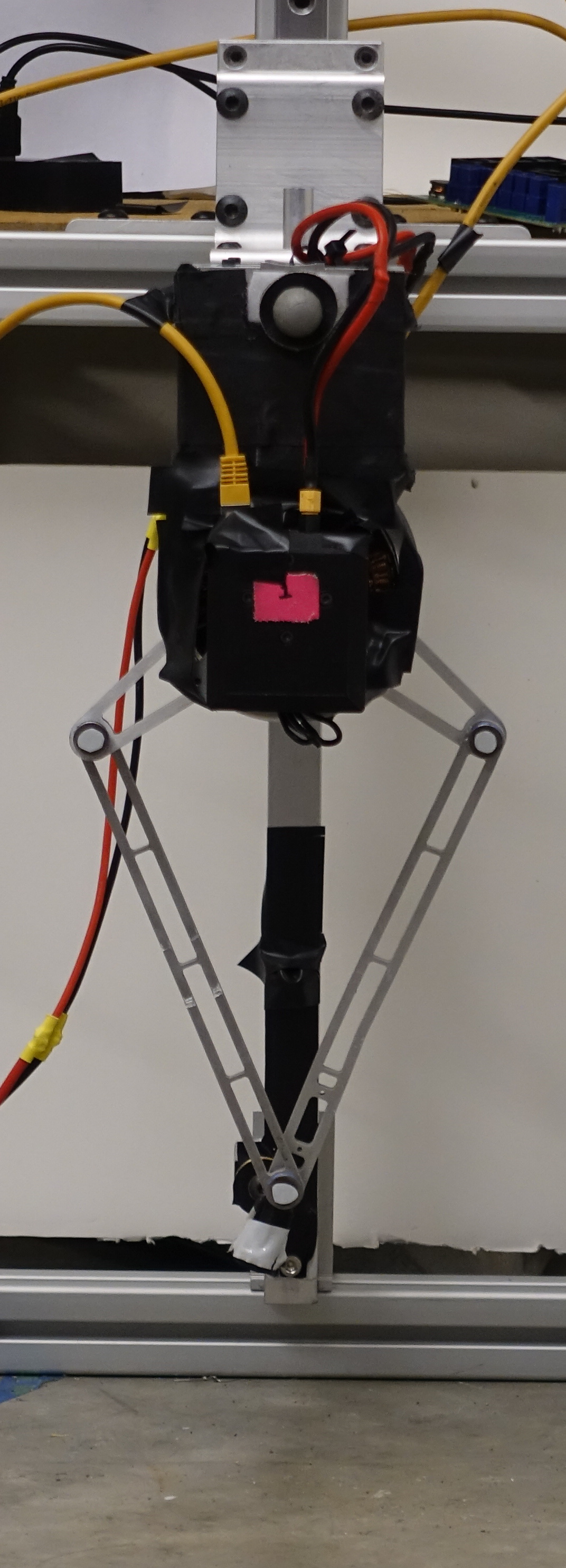
(a)

(b)

(c)

Figure 1: Jumping robot and impact oscillator hybrid system models (Sec. 4.1). (1(a)) Photograph of the physical robot (one leg from a Minitaur [23]) that inspired the simulation models. (1(b)) Nonlinear model consisting of two masses coupled with a linear spring and a nonlinear pantograph mechanism. (1(c)) Linear model consisting of two masses coupled with a linear spring.

We perform two sets of experiments. The first set of experiments in Sec. 4.2 concern the piecewise-linear model depicted in Figure 1(c) and explore the consequences of our modelling assumptions and the efficacy of our proposed algorithm:

• Sec. 4.2.1 demonstrates the advantage of employing a Student’s $t$ distribution for process noise as compared to a Gaussian distribution;

• Sec. 4.2.2 demonstrates the superior convergence rate yielded by Gauss-Newton descent directions as compared to gradient (steepest) descent;

• Sec. 4.2.3 demonstrates the advantage of smoothing the relaxed discrete state estimate; and

• Sec. 4.2.4 demonstrates the algorithm’s performance when onboard measurements are used instead of offboard measurements.

The second set of experiments in Sec. 4.3 evaluate our proposed approach using the nonlinear model depicted in Figure 1(b).

Since this section is devoted to comparing estimated states to ground truth simulation results, and since our approach entails the determination of a relaxed discrete state estimate en route to obtaining the discrete state estimate, we now introduce notation that distinguishes these quantities:

• $w_{t}$ $\in\mathcal{D}^{M}$ denotes the ground truth discrete state;

• $\widetilde{w}_{t}$ $\in\Delta^{M}$ denotes the relaxed discrete state estimate;

• $\widehat{w}_{t}$ $\in\mathcal{D}^{M}$ denotes the discrete state estimate.

This notational distinction was not introduced previously in the interest of readability since there was no ambiguity entailed by overloading notation in the problem formulation and algorithm specification.

4.1 Impact oscillator hybrid system models

The continuous state $x=(q,\dot{q})\in\mathbb{R}^{4}$ for the jumping robot hybrid system model consists of the two-dimensional configuration vector $q\in\mathbb{R}^{2}$ and corresponding velocity $\dot{q}\in\mathbb{R}^{2}$, where $q[1]$ and $q[2]$ denote the vertical height of the hip and foot, respectively. The foot is not permitted to penetrate the ground, $q[2]\geq 0$, so the first part of the discrete state indicates whether this constraint is active: A (air) if $q[2]>0$, G (ground) if $q[2]=0$. To compensate for energy losses at impact, an event-triggered controller stiffens or softens a spring based on which direction the hip is traveling, so the second part of the discrete state indicates the direction of travel for $q[1]$: $\uparrow$ if up, $\downarrow$ if down. With $\ddot{q}_{m}(q,\dot{q})\in\mathbb{R}^{2}$ denoting the acceleration of the hip and foot in discrete state $m\in\left\{\text{A}\!\downarrow,\text{G}\!\downarrow,\text{G}\!\uparrow,\text{A}\!\uparrow\right\}$, formulae for this acceleration are given in Table 1. At the moment of impact (when the discrete state changes from $w_{t}\in\{\text{A}\!\downarrow,\text{A}\!\uparrow\}$ to $w_{t+1}\in\{\text{G}\!\downarrow,\text{G}\!\uparrow\}$) the foot velocity $\dot{q}[2]$ is instantaneously reset to $0$, corresponding to perfectly plastic impact. An example of the jump in continuous state when transitioning from $\text{A}\!\downarrow$ to $\text{G}\!\downarrow$ on the foot velocity $\dot{q}[2]$ is shown in Figure 2 near time 17.5s.

Discrete state $w$	Icon	$\ddot{q}_{w}(x)$
$w=\text{A}\!\downarrow$		$\begin{bmatrix}\frac{1}{m_{h}}\left(-k_{1}(q,\dot{q})\right)-g\\ \frac{1}{m_{t}}\left(k_{1}(q,\dot{q})\right)-g\\ \end{bmatrix}$
$w=\text{G}\!\downarrow$		$\begin{bmatrix}\frac{1}{m_{h}}\left(-k_{1}(q,\dot{q})\right)-g\\ 0\\ \end{bmatrix}$
$w=\text{G}\!\uparrow$		$\begin{bmatrix}\frac{1}{m_{h}}\left(-k_{2}(q,\dot{q})\right)-g\\ 0\\ \end{bmatrix}$
$w=\text{A}\!\uparrow$		$\begin{bmatrix}\frac{1}{m_{h}}\left(-k_{2}(q,\dot{q})\right)-g\\ \frac{1}{m_{t}}\left(k_{2}(q,\dot{q})\right)-g\\ \end{bmatrix}$

Table 1: Discrete states and continuous dynamics for impact oscillator hybrid system models (Sec. 4.1). Note that the continuous dynamics $\ddot{q}$ have the same general form for both the piecewise-linear and -nonlinear models, with the spring law $k$ being a linear or nonlinear function of the continuous state $x=(q,\dot{q})$ depending on which model is considered.

4.2 Piecewise-linear impact oscillator experiment

In this subsection, we employ the linear spring laws

$$k_{1}(q,\dot{q})=10(q[1]-q[2])-3,$$

$$k_{2}(q,\dot{q})=15(q[1]-q[2])-3,$$

with parameter values $m_{h}=3,m_{t}=1,g=2$.

In our first demonstration the observed states are $q[1]$ and $q[2]$, position of the hip and foot, leaving the velocities unobserved:

$$\mathcal{H}_{\text{pos}}(x)=q.$$ (12)

State estimation results for this system are shown in Figure 5.

In the remainder of this subsection, we demonstrate the effects of the choices we made in our problem formulation (Sec. 2) and algorithm derivation (Sec. 3) using the piecewise-linear model as a running example. We also consider a variation where the measurements correspond to the leg length and velocity, which are more representative of the onboard measurements available to an autonomous robot operating outside of the laboratory.

4.2.1 Student’s $t$ versus Gaussian process noise

Figure 2 compares the estimation of foot velocity using Student’s $t$ with $r=0.01$ versus using Gaussian for the process noise distribution; in both cases the true discrete state is given. The estimated trajectory for both distributions match the true simulated trajectory away from jumps, while near jumps, such as around times $16.6$s and $17.5$s, using the Student’s $t$ distribution enables closer tracking of the instantaneous change in the true foot velocity $\dot{q}[2]$ than when using a Gaussian distribution.

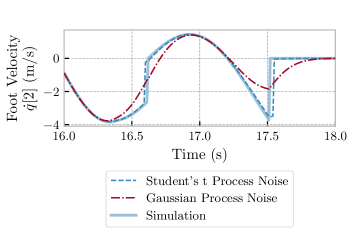
Figure 2: The Student’s $t$ distribution process noise yields better estimates of instantaneous changes in continuous state (Sec. 4.2.1). In this plot, estimates of the foot velocity are shown near two impacts ($\approx 16.6$s, $17.5$s).

4.2.2 Gauss-Newton versus gradient (steepest) descent

We empirically compared convergence rates for continuous state $x_{t}$ updates obtained using Gauss-Newton and gradient (steepest) descent directions (Algorithm 1, line 3). Figure 3 shows the log loss versus algorithm iteration for the two methods; the actual discrete state $w_{t}$ was taken as given to perform this comparison. As expected, the objective value decreases significantly faster when the search direction is determined by the Gauss-Newton scheme as compared to the direction of steepest descent, reaching the stopping criterion in ten times fewer iterations in our tests.

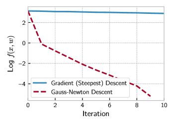
Figure 3: Gauss-Newton descent directions yield faster convergence than gradient (steepest) descent (Sec. 4.2.2). In this plot, the discrete state variables $w$ are given and the second line of Algorithm 1 is modified to use either Gauss-Newton descent directions or gradient (steepest) descent to estimate the continuous state variables $x$ by minimizing the relaxed objective function $f(x,w)$ (4).

4.2.3 Smoothing the relaxed discrete state versus not

If the continuous states are given, the discrete state estimate returned by our algorithm (skipping lines 2 and 3 of Algorithm 1) is very close to the true discrete state regardless of whether a smoothing term is included in the relaxed problem formulation. When simultaneously estimating both the continuous and discrete states, the smoothing term becomes crucial, as illustrated by comparing the discrete state estimates ($\widehat{w}_{t}$) in Figure 4 (without smoothing) and Figure 5 (with smoothing). In particular, the estimated discrete state switches rapidly without smoothing, whereas with smoothing the discrete state tends to remain constant for many samples and change mostly near ground-truth switching times.

Figure 4: Without smoothing ($\nu=0$), the discrete state estimate switches frequently (Sec. 4.2.3). The top plot shows the true discrete state of the system $w\in D^{M}$, the relaxed discrete state estimate $\widetilde{w}\in\Delta^{M}$, and the discrete state estimate $\widehat{w}\in D^{M}$ for a simulation of the piecewise-linear system. The subsequent plots show the estimate, simulation, and error $\epsilon$ values for position and velocity of the hip and foot.

Figure 5: With smoothing ($\nu>0$), the discrete state estimate mostly switches near the true switching times. (Sec. 4.2.3). This plot shows results from the piecewise-linear system; the notational and plotting conventions are adopted from Figure 4.

4.2.4 Onboard versus offboard measurements

In the laboratory, the positions of the robot hip and foot can be directly measured offboard, e.g. with an external camera system. Outside of the laboratory, only the relative position of the hip and foot can be directly measured onboard our robot. Thus, we are motivated by this practical consideration to evaluate our algorithm’s performance in the case where only the relative position and velocity of the hip and foot are measured,

$$\mathcal{H}_{\text{relative}}(x)=\begin{bmatrix}q[1]-q[2]\\ \dot{q}[1]-\dot{q}[2]\end{bmatrix}.$$ (13)

Although the full hybrid system state is formally unobservable with these relative measurements, our algorithm nevertheless yields good estimates of the discrete state as shown in Figure 6; due to large errors in the estimate of (unobservable) continuous states, we omit those results from the figure.

Figure 6: Estimated discrete state using onboard (relative position and velocity) measurements $\mathcal{H}_{\text{relative}}$ (13) for the piecewise-linear system closely matches true discrete state. (Sec. 4.2.4). Continuous state estimates are not shown since they are formally unobservable using only onboard measurements (in practice, they drift away from ground truth over time).

4.3 Piecewise-nonlinear impact oscillator experiment

To test Algorithm 1 on a nonlinear model, we included the kinematic constraints depicted in Figure 1(b), resulting in a nonlinear spring force. In this model we set the two spring laws to be the same $k_{1}=k_{2}$, decreasing the number of discrete states from four to two: $w=\text{A}$ when $q[2]>0$ and $w=\text{G}$ when $q[2]=0$. State estimation results compare favorably with the analogous results from the piecewise-linear system when using either absolute position measurements $\mathcal{H}_{\text{pos}}$ (12) (compare Figure 7 with Figure 5) or relative measurements $\mathcal{H}_{\text{relative}}$ (13) (compare Figure 8 with Figure 6).

In Figure 7 we see that the model can estimate continuous and discrete states in the nonlinear setting. However, we do notice that the estimated trajectories are not as close to ground truth as in the linear case. In particular, when $q[2]$ has a value only slightly greater than 0 (e.g. between times 3s and 4s), the algorithm fails to detect the transition between $w=\text{A}$ and $w=\text{G}$.

Figure 7: Continuous and discrete states estimated for the piecewise-nonlinear model (Sec. 4.3). Notational and plotting conventions are adopted from Figure 4; note that this model only has two discrete states (Sec. 4.1).

Figure 8: Estimated discrete state using onboard (relative position and velocity) measurements $\mathcal{H}_{\text{relative}}$ (13) for the piecewise-nonlinear system closely matches true discrete state. (Sec. 4.2.4). As with Figure 6, continuous state estimates are not shown since they drift from the true values over time; note that this nonlinear model only has two discrete states (Sec. 4.1).

5 Conclusion

We proposed a new state estimation algorithm for hybrid systems, analyzed its convergence properties, and evaluated its performance on piecewise-linear and -nonlinear hybrid systems with non-identity resets. The algorithm leverages a relaxed state estimation problem formulation where the decision variables corresponding to the discrete state are allowed to take on continuous values. This relaxation yields a continuous optimization problem that can be solved using recently-developed nonsmooth variable projection techniques. The effectiveness of the approach was demonstrated on hybrid system models of mechanical systems undergoing impact.

References

- [1] A. Alessandri, M. Baglietto, and G. Battistelli. Receding-horizon estimation for switching discrete-time linear systems. IEEE Transactions on Automatic Control, 50(11):1736–1748, November 2005.
- [2] Angelo Alessandri, Marco Baglietto, and Giorgio Battistelli. Minimum-Distance Receding-Horizon State Estimation for Switching Discrete-Time Linear Systems. In Rolf Findeisen, Frank Allgöwer, and Lorenz T. Biegler, editors, Assessment and Future Directions of Nonlinear Model Predictive Control, number 358 in Lecture Notes in Control and Information Sciences, pages 348–366. Springer-Verlag Berlin Heidelberg, 2007.
- [3] A. Y. Aravkin, J. V. Burke, L. Ljung, A. Lozano, and G. Pillonetto. Generalized Kalman Smoothing: Modeling and Algorithms. arXiv:1609.06369 [math, stat], September 2016.
- [4] Aleksandr Aravkin, James V. Burke, and Gianluigi Pillonetto. Robust and Trend-following Kalman Smoothers using Student’s t. IFAC Proceedings Volumes, 45(16):1215–1220, July 2012.
- [5] Aleksandr Aravkin, Dmitriy Drusvyatskiy, and Tristan van Leeuwen. Variable projection without smoothness. arXiv preprint arXiv:1601.05011, 2016.
- [6] Aleksandr Y Aravkin, James V Burke, and Gianluigi Pillonetto. Robust and trend-following student’s t kalman smoothers. SIAM Journal on Control and Optimization, 52(5):2891–2916, 2014.
- [7] Laurent Bako and Stéphane Lecoeuche. A sparse optimization approach to state observer design for switched linear systems. Systems & Control Letters, 62(2):143–151, February 2013.
- [8] A. Balluchi, L. Benvenuti, M.D. Di Benedetto, and A.L. Sangiovanni-Vincentelli. Observability for hybrid systems. In 42nd IEEE International Conference on Decision and Control (IEEE Cat. No.03CH37475), volume 2, pages 1159–1164. IEEE, 2003.
- [9] Andrea Balluchi, Luca Benvenuti, Maria D. Di Benedetto, and Alberto Sangiovanni-Vincentelli. The design of dynamical observers for hybrid systems: Theory and application to an automotive control problem. Automatica, 49(4):915–925, 2013.
- [10] Andrea Balluchi, Luca Benvenuti, Maria D. Di Benedetto, and Alberto L. Sangiovanni-Vincentelli. Design of Observers for Hybrid Systems. In Gerhard Goos, Juris Hartmanis, Jan van Leeuwen, Claire J. Tomlin, and Mark R. Greenstreet, editors, Hybrid Systems: Computation and Control, volume 2289, pages 76–89. Springer Berlin Heidelberg, Berlin, Heidelberg, 2002.
- [11] N. Barhoumi, F. Msahli, M. Djemaï, and K. Busawon. Observer design for some classes of uniformly observable nonlinear hybrid systems. Nonlinear Analysis: Hybrid Systems, 6(4):917–929, 2012.
- [12] Amir Beck and Marc Teboulle. A fast iterative shrinkage-thresholding algorithm for linear inverse problems. SIAM Journal on Imaging Sciences, 2(1):183–202, 2009.
- [13] A. Bemporad, D. Mignone, and M. Morari. Moving horizon estimation for hybrid systems and fault detection. In Proceedings of the 1999 American Control Conference (Cat. No. 99CH36251), volume 4, pages 2471–2475 vol.4, June 1999.
- [14] H. A. P. Blom and E. A. Bloem. Exact Bayesian and particle filtering of stochastic hybrid systems. IEEE Transactions on Aerospace and Electronic Systems, 43(1):55–70, 2007.
- [15] James V Burke. Descent methods for composite nondifferentiable optimization problems. Mathematical Programming, 33(3):260–279, 1985.
- [16] M. Di Bernardo, editor. Piecewise-Smooth Dynamical Systems: Theory and Applications. Number 163 in Applied Mathematical Sciences. Springer, London, 2008. OCLC: ocn144515657.
- [17] A. Doucet, N. J. Gordon, and V. Krishnamurthy. Particle filters for state estimation of jump Markov linear systems. IEEE Transactions on Signal Processing, 49(3):613–624, 2001.
- [18] Nima Fazeli, Samuel Zapolsky, Evan Drumwright, and Alberto Rodriguez. Learning Data-Efficient Rigid-Body Contact Models: Case Study of Planar Impact. In Proceedings of the 1st Annual Conference on Robot Learning, page 10, 2017.
- [19] G. Ferrari-Trecate, D. Mignone, and M. Morari. Moving horizon estimation for hybrid systems. IEEE Transactions on Automatic Control, 47(10):1663–1676, October 2002.
- [20] D. Gómez-Gutiérrez, S. Čelikovský, A. Ramírez-Treviño, J. Ruiz-Léon, and S. Di Gennaro. Sliding mode observer for Switched Linear Systems. In 2011 IEEE International Conference on Automation Science and Engineering, pages 725–730, 2011.
- [21] J. P. Hespanha and A. S. Morse. Stability of switched systems with average dwell-time. In Proceedings of the 38th IEEE Conference on Decision and Control (Cat. No.99CH36304), volume 3, pages 2655–2660 vol.3, December 1999.
- [22] Scott C Johnson. Observability and Observer Design for Switched Linear Systems. PhD thesis, Purdue University, December 2016.
- [23] Gavin Kenneally, Avik De, and D. E. Koditschek. Design Principles for a Family of Direct-Drive Legged Robots. IEEE Robotics and Automation Letters, 1(2):900–907, July 2016.
- [24] Per Lötstedt. Mechanical Systems of Rigid Bodies Subject to Unilateral Constraints. SIAM Journal on Applied Mathematics, 42(2):281–296, 1982.
- [25] L. Menini and A. Tornambe. Asymptotic tracking of periodic trajectories for a simple mechanical system subject to nonsmooth impacts. IEEE Transactions on Automatic Control, 46(7):1122–1126, July 2001.
- [26] Jorge Nocedal and Stephen J Wright. Nonlinear Equations. Springer, 2006.
- [27] R. Tyrrell Rockafellar and Roger J.-B. Wets. Variational Analysis. Springer Verlag, Heidelberg, Berlin, New York, 1998.
- [28] M Schatzman. Uniqueness and continuous dependence on data for one–dimensional impact problems. Mathematical and computer modelling, 28(4—8):1–18, 1998.
- [29] C E Seah and I Hwang. State estimation for stochastic linear hybrid systems with Continuous-State-Dependent transitions: An IMM approach. IEEE transactions on aerospace and electronic systems, 45(1):376–392, January 2009.
- [30] Robert R. Stengel. Optimal Control and Estimation. Dover, 1994.