On LSE in regression model for long-range dependent random fields on spheres.

\nameVo Anha,b, Andriy Olenkoc and Volodymyr Vaskovychc CONTACT Andriy Olenko. Email: a.olenko@latrobe.edu.au aSchool of Mathematical Sciences, Queensland University of Technology, Brisbane, Queensland, 4001, Australia
bFaculty of Science, Engineering and Technology, Swinburne University of Technology, Victoria, 3122, Australia
cDepartment of Mathematics and Statistics, La Trobe University, Melbourne, 3086, Australia
Abstract

We study the asymptotic behaviour of least squares estimators in regression models for long-range dependent random fields observed on spheres. The least squares estimator can be given as a weighted functional of long-range dependent random fields. It is known that in this scenario the limits can be non-Gaussian. We derive the limit distribution and the corresponding rate of convergence for the estimators. The results were obtained under rather general assumptions on the random fields. Simulation studies were conducted to support theoretical findings.

keywords:
Spatial regression, LSE, Long-range dependence, Non-central limit theorems, Hermite-type distribution.
{amscode}

62H11, 62J05, 60G60.

1 Introduction

Studying the asymptotic behavior of the regression parameter estimators is an important topic in Spatial Statistics, see [1], [2], [3]. A potential area of application of the results in this paper is cosmology, and more specifically, models involving the cosmic microwave background (CMB). The recent data obtained by the Wilkinson Microwave Anisotropy Probe and Planck missions, combined with data that will be obtained during the future missions, will allow to predict the behaviour of CMB at increasing distances that are far beyond the reach of any modern telescopes. Another area of application is studying the porosity of mineral resources, see, for example, [4] about data and analysis of the porosity of hydrocarbon reservoirs. Some other potential applications of the model discussed in this article might involve 3D rupture models, soil fertility and paleomagnetism.

One of the first works that developed statistical theory of random fields was the book by [5]. Direct probability techniques for models involving random fields were proposed and various estimators of regression parameters were investigated. The asymptotic behaviour of some of these estimators was studied in [6]. Both Gaussian and non-Gaussian limits were obtained for particular models. No results about rates of convergence were given.

In this paper we consider the regression model ξ(x)=ah(x)+ψ(x)𝜉𝑥𝑎𝑥𝜓𝑥\xi(x)=ah(x)+\psi(x), where h()h(\cdot) is a known deterministic function, a𝑎a is an unknown parameter and the error ψ()𝜓\psi(\cdot) is a random field. For results concerning such regression models see [7] and references therein. Since there are numerous situations in practice when random processes and fields are non-Gaussian, we consider a particular case when ψ()𝜓\psi(\cdot) is a non-linear function of a Gaussian random field. Such random fields are very common in non-Gaussian modeling since they can be analyzed using Wiener chaos expansions and in many cases offer a good data approximation, see [8, 9]. In this article, we consider the underlying Gaussian random fields to be long-range dependent.

Long-range dependence is a well-established phenomenon that can be observed in various fields such as hydrology, agriculture, image analysis, earth sciences, cosmology, just to name a few. For this reason, models involving long-range dependent random fields have been an object of statistical interest for years, see [10, 11, 12, 13].

Various earth science and cosmology applications require studying random fields defined on surfaces, for example, see [14, 15]. In this paper we consider random fields that are defined on expanding spheres. One can find detailed information about such spherical random fields in [16, 5].

The regression model studied in this paper was first considered in [5]. For this model the best linear unbiased estimator (BLUE) of the unknown parameter a𝑎a was derived. In [17] the least squares estimator (LSE) of a𝑎a was obtained. Its mean-square efficiency was compared to BLUE and it was shown that, apart from some degenerate cases, LSE is less efficient than BLUE. However, for most functions h()h(\cdot) BLUE is much more difficult to compute than LSE. For this reason using LSE is preferable to BLUE in practice. No results concerning limit distributions of the regression parameter estimators were obtained in [17, 5] or other literature known to the authors. This article investigates the limit distribution of LSE and its rate of convergence.

For the particular case h()11h(\cdot)\equiv 1, some approaches to study non-linear functionals of random fields on surfaces and rates of convergence were proposed in [18]. This article shows how the methodology developed in [18] can be extended to the general case of weighted non-linear functionals of random fields, i.e. the case of arbitrary functions h()h(\cdot). To reduce repetitions to a minimum, in this article we present only those parts of proofs that are new or require modifications of results in [18].

The main goal of this article is to demonstrate potential applications of the developed methodology to statistical problems. We focus on the LSE for a regression model, however there are numerous other statistical problems that can be studied using weighted non-linear functionals of random fields. For example, by choosing the appropriate integrand functions, various characteristics of random fields, such as moments, can be represented by the considered functionals. In [18] it was shown that Minkowski functionals can be obtained by choosing indicator functions as the integrands. Another important statistical application is assigning different weights to different observation regions. In spatial statistics it is often used to control the edge effects. Also, assigning weights to observations or observation regions is an important case of data tapering that is often used to reduce effects of less reliable observations.

Section 5 presents detailed simulation studies that back up the theory and suggest new research questions. To the best of our knowledge, simulation studies have not been done in the available literature on convergence rates in non-central limit theorems for long-range dependent random fields. The numerical study suggests that the exponential rate of convergence obtained in all known theoretical studies might be improved. For the cases of a sphere and a cube, various observation windows and weight functions were investigated. The detailed methodology for practical simulations and studying weighted functionals of random fields observed on surfaces is provided. The corresponding R codes for one-core and parallel computing are freely available on-line and can be used by researchers in this field.

To obtain the main results some fine properties of the Fourier transforms on surfaces are employed. Note that the Fourier transforms were more frequently studied on solid bodies than on surfaces. The assumptions for obtaining the required rate of decay are weaker in the case of solid bodies. Therefore, all results derived in this article can be analogously obtained for solid bodies.

As mentioned earlier, to study the asymptotic behaviour of LSE we investigate weighted non-linear functionals of Gaussian random fields. Non-linear functionals of random processes were considered in [6, 19]. In [6] only the case of short-range dependent random processes and Gaussian asymptotics for weighted functionals was studied. In [19] non-Gaussian asymptotics were obtained for long-range dependent random processes. The results in [19] can be obtained from the methodology of this article as random processes can be considered as random fields indexed by a one-dimensional Euclidean space. For random fields and the simplest particular case h()11h(\cdot)\equiv 1 it was shown that the functionals can produce non-Gaussian limits, see [20, 21, 22]. The more detailed overview of this particular case was given in [23]. In the general case, weighted linear functionals of the Gaussian random fields were studied in [24]. The assumptions on weighted functions used in this article are weaker than those used in [24]. Moreover, we do not apply any conditions on Fourier transforms of weight functions. The known Gaussian asymptotics are a particular case when integrand functions are linear. None of the above studies provided the rate of convergence to the obtained limits. To the best of our knowledge, this paper is the first work that provides the rate of convergence for weighted functionals and LSE of long-range dependent random fields on hypersurfaces.

The article is organized as follows. In Section 2 we recall some basic definitions of the spectral theory of random fields. Section 3 presents the model and states the results. Proofs of the results are provided in Section 4. In Section 5 some simulation studies are presented to confirm theoretical findings. Conclusions and directions for future research are stated in Section 6.

2 Definitions

In this section we provide the main definitions that are used in this article.

In what follows |||\cdot| and \|\cdot\| denote the Lebesgue measure and the Euclidean distance in dsuperscript𝑑\mathbb{R}^{d}, d2𝑑2d\geq 2, respectively. Let B(y,s)𝐵𝑦𝑠B(y,s) be a d𝑑d-dimensional ball with centre y𝑦y and radius s𝑠s, and let S(r)𝑆𝑟S(r) be a (d1)𝑑1(d-1)-dimensional sphere in dsuperscript𝑑\mathbb{R}^{d} with the centre at the origin and radius r𝑟r. We use the symbols C𝐶C and δ𝛿\delta to denote constants which are not important for our exposition. Moreover, the same symbol may be used for different constants appearing in the same proof.

Let (Ω,,P)Ω𝑃(\Omega,\mathcal{F},P) be a complete probability space and let Td𝑇superscript𝑑T\subseteq\mathbb{R}^{d} be a set.

Definition 1.

[12] A random field is a function η(w,x):Ω×T:𝜂𝑤𝑥Ω𝑇\eta(w,x):\Omega\times T\rightarrow\mathbb{R} such that η(w,x)𝜂𝑤𝑥\eta(w,x) is a random variable for any xT𝑥𝑇x\in T. It will also be denoted as η(x),xT.𝜂𝑥𝑥𝑇\eta(x),\ x\in T.

Definition 2.

[12] A random field satisfying 𝐄η2(x)<𝐄superscript𝜂2𝑥\mathbf{E}\eta^{2}(x)<\infty is called homogeneous in the wide sense if its mathematical expectation m(x)=𝐄η(x)𝑚𝑥𝐄𝜂𝑥m(x)=\mathbf{E}\eta(x) and covariance function B(x,y)=𝐄[η(x)m(x)][η(y)m(y)]B𝑥𝑦𝐄delimited-[]𝜂𝑥𝑚𝑥delimited-[]𝜂𝑦𝑚𝑦{\rm{B}}(x,y)={\mathbf{E}}\left[\eta(x)-m(x)\right]\left[\eta(y)-m(y)\right] are invariant with respect to the group of shifts τ𝜏\tau in dsuperscript𝑑\mathbb{R}^{d}, that is, m(x)=m(x+τ)𝑚𝑥𝑚𝑥𝜏m(x)=m(x+\tau), B(x,y)=B(x+τ,y+τ)B𝑥𝑦B𝑥𝜏𝑦𝜏{\rm{B}}(x,y)={\rm{B}}(x+\tau,y+\tau) for any x,yT𝑥𝑦𝑇x,y\in T.

It means that 𝐄η(x)=c=const𝐄𝜂𝑥𝑐𝑐𝑜𝑛𝑠𝑡\mathbf{E}\eta(x)=c=const, and the covariance B(x,y)B𝑥𝑦{\rm{B}}(x,y) depends only on the difference xy𝑥𝑦x-y.

Definition 3.

[12] A random field satisfying 𝐄η2(x)<𝐄superscript𝜂2𝑥\mathbf{E}\eta^{2}(x)<\infty is called isotropic in the wide sense if its mathematical expectation m(x)𝑚𝑥m(x) and covariance function B(x,y)B𝑥𝑦{\rm{B}}(x,y) are invariant with respect to rotations.

In this article homogeneity and isotropy in the wide sense will be simply called homogeneity and isotropy.

Let us consider a measurable mean-square continuous zero-mean homogeneous isotropic real-valued random field η(x),xd,𝜂𝑥𝑥superscript𝑑\eta(x),\ x\in\mathbb{R}^{d}, defined on a probability space (Ω,,P),Ω𝑃(\Omega,\mathcal{F},P), with the covariance function

B(r):=Cov(η(x),η(y))=0Yd(rz)dΦ(z),x,yd,formulae-sequenceassignB𝑟Cov𝜂𝑥𝜂𝑦superscriptsubscript0subscript𝑌𝑑𝑟𝑧differential-dΦ𝑧𝑥𝑦superscript𝑑\text{\rm{B}}(r):=\mathrm{Cov}\left(\eta(x),\eta(y)\right)=\int_{0}^{\infty}Y_{d}(rz)\,\mathrm{d}\Phi(z),\ x,y\in\mathbb{R}^{d},

where r:=xy,assign𝑟norm𝑥𝑦r:=\left\|x-y\right\|, Φ()Φ\Phi(\cdot) is the isotropic spectral measure, the function Yd()subscript𝑌𝑑Y_{d}(\cdot) is defined by

Yd(z):=2(d2)/2Γ(d2)J(d2)/2(z)z(2d)/2,z0,formulae-sequenceassignsubscript𝑌𝑑𝑧superscript2𝑑22Γ𝑑2subscript𝐽𝑑22𝑧superscript𝑧2𝑑2𝑧0Y_{d}(z):=2^{(d-2)/2}\Gamma\left(\frac{d}{2}\right)\ J_{(d-2)/2}(z)\ z^{(2-d)/2},\quad z\geq 0,

and J(d2)/2()subscript𝐽𝑑22J_{(d-2)/2}(\cdot) is the Bessel function of the first kind of order (d2)/2.𝑑22(d-2)/2.

Definition 4.

The random field η(x),𝜂𝑥\eta(x), xd,𝑥superscript𝑑x\in\mathbb{R}^{d}, defined above is said to possess an absolutely continuous spectrum if there exists a function f()𝑓f(\cdot) such that

Φ(z)=2πd/2Γ1(d/2)0zud1f(u)du,z0,ud1f(u)L1(+).formulae-sequenceΦ𝑧2superscript𝜋𝑑2superscriptΓ1𝑑2superscriptsubscript0𝑧superscript𝑢𝑑1𝑓𝑢differential-d𝑢formulae-sequence𝑧0superscript𝑢𝑑1𝑓𝑢subscript𝐿1subscript\Phi(z)=2\pi^{d/2}\Gamma^{-1}\left(d/2\right)\int_{0}^{z}u^{d-1}f(u)\,\mathrm{d}u,\quad z\geq 0,\quad u^{d-1}f(u)\in L_{1}(\mathbb{R}_{+}).

The function f()𝑓f(\cdot) is called the isotropic spectral density function of the field η(x).𝜂𝑥\eta(x). The field η(x)𝜂𝑥\eta(x) with an absolutely continuous spectrum has the following representation

η(x)=dei<λ,x>f(λ)W(dλ),𝜂𝑥subscriptsuperscript𝑑superscript𝑒𝑖𝜆𝑥𝑓norm𝜆𝑊d𝜆\eta(x)=\int_{\mathbb{R}^{d}}e^{i<\lambda,x>}\sqrt{f\left(\left\|\lambda\right\|\right)}W(\mathrm{d}\lambda),

where W()𝑊W(\cdot) is the complex Gaussian white noise random measure on d.superscript𝑑\mathbb{R}^{d}.

Let Hk(u)subscript𝐻𝑘𝑢H_{k}(u), k0𝑘0k\geq 0, u𝑢u\in\mathbb{R}, be the Hermite polynomials, see [25]. These polynomials form a complete orthogonal system in the Hilbert space

L2(,ϕ(w)dw)={G:G2(w)ϕ(w)dw<},ϕ(w):=12πew22.formulae-sequencesubscript𝐿2italic-ϕ𝑤𝑑𝑤conditional-set𝐺subscriptsuperscript𝐺2𝑤italic-ϕ𝑤differential-d𝑤assignitalic-ϕ𝑤12𝜋superscript𝑒superscript𝑤22{L}_{2}(\mathbb{R},\phi(w)\,dw)=\left\{G:\int_{\mathbb{R}}G^{2}(w)\phi(w)\,\mathrm{d}w<\infty\right\},\quad\phi(w):=\frac{1}{\sqrt{2\pi}}e^{-\frac{w^{2}}{2}}.

An arbitrary function GL2(,ϕ(w)dw)𝐺subscript𝐿2italic-ϕ𝑤𝑑𝑤G\in{L}_{2}(\mathbb{R},\phi(w)\,dw) admits the mean-square convergent expansion

G(w)=j=0CjHj(w)j!,Cj:=G(w)Hj(w)ϕ(w)dw.formulae-sequence𝐺𝑤superscriptsubscript𝑗0subscript𝐶𝑗subscript𝐻𝑗𝑤𝑗assignsubscript𝐶𝑗subscript𝐺𝑤subscript𝐻𝑗𝑤italic-ϕ𝑤differential-d𝑤G(w)=\sum_{j=0}^{\infty}\frac{C_{j}H_{j}(w)}{j!},\qquad C_{j}:=\int_{\mathbb{R}}G(w)H_{j}(w)\phi(w)\,\mathrm{d}w.

By Parseval’s identity

j=0Cj2j!=G2(w)ϕ(w)dw.superscriptsubscript𝑗0superscriptsubscript𝐶𝑗2𝑗subscriptsuperscript𝐺2𝑤italic-ϕ𝑤differential-d𝑤\sum_{j=0}^{\infty}\frac{C_{j}^{2}}{j!}=\int_{\mathbb{R}}G^{2}(w)\phi(w)\,\mathrm{d}w.

It will be shown that studying asymptotics of non-linear functionals defined by a function GL2(,ϕ(w)dw)𝐺subscript𝐿2italic-ϕ𝑤𝑑𝑤G\in{L}_{2}(\mathbb{R},\phi(w)\,dw) can be done by investigating leading terms in their expansions. The following definitions and remarks provide basic notations and tools to formulate and prove these asymptotic results.

Definition 5.

[21] Let GL2(,ϕ(w)dw)𝐺subscript𝐿2italic-ϕ𝑤𝑑𝑤G\in{L}_{2}(\mathbb{R},\phi(w)\,dw) and assume there exists an integer κ𝜅\kappa\in\mathbb{N} such that Cj=0subscript𝐶𝑗0C_{j}=0, for all 0jκ1,0𝑗𝜅10\leq j\leq\kappa-1, but Cκ0.subscript𝐶𝜅0C_{\kappa}\neq 0. Then κ𝜅\kappa is called the Hermite rank of G()𝐺G(\cdot) and is denoted by HrankG.𝐻rank𝐺H\mbox{rank}\,G.

The following remark gives a well known property of Hermite polynomials of Gaussian vectors, see [12].

Remark 1.

If (ξ1,,ξ2p)subscript𝜉1subscript𝜉2𝑝(\xi_{1},\ldots,\xi_{2p}) is a 2p2𝑝2p-dimensional zero-mean Gaussian vector with

𝐄ξjξk={1,if k=j,rj,if k=j+pand 1jp,0,otherwise,𝐄subscript𝜉𝑗subscript𝜉𝑘cases1if 𝑘𝑗subscript𝑟𝑗if 𝑘𝑗𝑝and 1𝑗𝑝0otherwise,\mathbf{E}\xi_{j}\xi_{k}=\begin{cases}1,&\mbox{if }k=j,\\ r_{j},&\mbox{if }k=j+p\ \mbox{and }1\leq j\leq p,\\ 0,&\mbox{otherwise,}\end{cases}

then

𝐄j=1pHkj(ξj)Hmj(ξj+p)=j=1pδkjmjkj!rjkj,𝐄superscriptsubscriptproduct𝑗1𝑝subscript𝐻subscript𝑘𝑗subscript𝜉𝑗subscript𝐻subscript𝑚𝑗subscript𝜉𝑗𝑝superscriptsubscriptproduct𝑗1𝑝superscriptsubscript𝛿subscript𝑘𝑗subscript𝑚𝑗subscript𝑘𝑗superscriptsubscript𝑟𝑗subscript𝑘𝑗\mathbf{E}\ \prod_{j=1}^{p}H_{k_{j}}(\xi_{j})H_{m_{j}}(\xi_{j+p})=\prod_{j=1}^{p}\delta_{k_{j}}^{m_{j}}\ k_{j}!\ r_{j}^{k_{j}}, (1)

where δkm={1,if k=m,0,if km,superscriptsubscript𝛿𝑘𝑚cases1if 𝑘𝑚0if 𝑘𝑚\delta_{k}^{m}=\begin{cases}1,&\mbox{if }k=m,\\ 0,&\mbox{if }k\neq m,\end{cases}  is the Dirac delta function.

Let ΔΔ\Delta be a bounded set in d,d2,superscript𝑑𝑑2\mathbb{R}^{d},\,d\geq 2, with a boundary ΔΔ\partial\Delta. Let Δ(r)Δ𝑟\Delta(r), r>0,𝑟0r>0, be the homothetic image of the set ΔΔ\Delta with the centre of homothety at the origin and the coefficient r>0𝑟0r>0, that is |Δ(r)|=rd|Δ|Δ𝑟superscript𝑟𝑑Δ|\Delta(r)|=r^{d}|\Delta|. Let σ()𝜎\sigma(\cdot) be the d1𝑑1d-1-dimensional Lebesgue measure on Δ(r)Δ𝑟\partial\Delta(r). Let U𝑈U and V𝑉V be two independent and uniformly distributed random vectors on the hypersurface Δ(r)Δ𝑟\partial\Delta(r). We denote by ψΔ(r)(ρ),subscript𝜓Δ𝑟𝜌\psi_{\Delta(r)}(\rho), ρ0,𝜌0\rho\geq 0, the probability density function of the distance UVnorm𝑈𝑉\left\|U-V\right\| between U𝑈U and V.𝑉V. Note that ψΔ(r)(ρ)=0subscript𝜓Δ𝑟𝜌0\psi_{\Delta(r)}(\rho)=0 if ρ>diam{Δ(r)}.𝜌𝑑𝑖𝑎𝑚Δ𝑟\rho>diam\left\{\partial\Delta(r)\right\}. Using the above notations, we obtain the representation

Δ(r)Δ(r)G(xy)σ(dx)σ(dy)=|Δ|2r2d2EG(UV)=subscriptΔ𝑟subscriptΔ𝑟𝐺norm𝑥𝑦𝜎d𝑥𝜎d𝑦superscriptΔ2superscript𝑟2𝑑2E𝐺norm𝑈𝑉absent\int\limits_{\partial\Delta(r)}\int\limits_{\partial\Delta(r)}G(\left\|x-y\right\|)\sigma({\rm d}x)\,\sigma({\rm d}y)=\left|\partial\Delta\right|^{2}r^{2d-2}\mathrm{E}\ G(\left\|U-V\right\|)=
=|Δ|2r2d20diam{Δ(r)}G(ρ)ψΔ(r)(ρ)𝑑ρ.absentsuperscriptΔ2superscript𝑟2𝑑2superscriptsubscript0𝑑𝑖𝑎𝑚Δ𝑟𝐺𝜌subscript𝜓Δ𝑟𝜌differential-d𝜌=\left|\partial\Delta\right|^{2}r^{2d-2}\int_{0}^{diam\left\{\partial\Delta(r)\right\}}G(\rho)\ \psi_{\Delta(r)}(\rho)d\rho. (2)

For various hypersurfaces ΔΔ\partial\Delta explicit expressions for ψΔ(r)()subscript𝜓Δ𝑟\psi_{\Delta(r)}(\cdot) are presented in [12]. In the case of spheres it takes the following form.

Remark 2.

If Δ(r)=S(r)Δ𝑟𝑆𝑟\partial\Delta(r)=S(r), then

ψΔ(r)(ρ)=1πΓ(d2)Γ1(d12)r1dρd2(1ρ24u2)d32,0<ρ<2r.formulae-sequencesubscript𝜓Δ𝑟𝜌1𝜋Γ𝑑2superscriptΓ1𝑑12superscript𝑟1𝑑superscript𝜌𝑑2superscript1superscript𝜌24superscript𝑢2𝑑320𝜌2𝑟\psi_{\Delta(r)}(\rho)=\frac{1}{\sqrt{\pi}}\Gamma\left(\frac{d}{2}\right)\Gamma^{-1}\left(\frac{d-1}{2}\right)r^{1-d}\rho^{d-2}\left(1-\frac{\rho^{2}}{4u^{2}}\right)^{\frac{d-3}{2}},\quad 0<\rho<2r.
Definition 6.

[26] A measurable function L:(0,)(0,):𝐿00L:(0,\infty)\rightarrow(0,\infty) is said to be slowly varying at infinity if for all t>0𝑡0t>0

limλL(λt)L(λ)=1.subscript𝜆𝐿𝜆𝑡𝐿𝜆1\lim\limits_{\lambda\rightarrow\infty}\frac{L(\lambda t)}{L(\lambda)}=1.

If L()𝐿L(\cdot) varies slowly, then raL(r),superscript𝑟𝑎𝐿𝑟r^{a}L(r)\rightarrow\infty, raL(r)0superscript𝑟𝑎𝐿𝑟0r^{-a}L(r)\rightarrow 0 for an arbitrary a>0𝑎0a>0 when r,𝑟r\rightarrow\infty, see Proposition 1.3.6 in [26].

Definition 7.

[26] A measurable function g:(0,)(0,):𝑔00g:(0,\infty)\rightarrow(0,\infty) is said to be regularly varying at infinity, denoted g()Rτ𝑔subscript𝑅𝜏g(\cdot)\in R_{\tau}, if there exists τ𝜏\tau such that, for all t>0,𝑡0t>0, it holds that

limλg(λt)g(λ)=tτ.subscript𝜆𝑔𝜆𝑡𝑔𝜆superscript𝑡𝜏\lim\limits_{\lambda\rightarrow\infty}\frac{g(\lambda t)}{g(\lambda)}=t^{\tau}.
Definition 8.

[26] Let g:(0,)(0,):𝑔00g:(0,\infty)\rightarrow(0,\infty) be a measurable function and g(x)0𝑔𝑥0g(x)\rightarrow 0 as x𝑥x\rightarrow\infty. A slowly varying function L()𝐿L(\cdot) is said to be slowly varying with remainder of type 2, or that it belongs to the class SR2, if

λ>1:L(λx)L(x)1k(λ)g(x),x,\forall\lambda>1:\quad\frac{L(\lambda x)}{L(x)}-1\sim k(\lambda)g(x),\quad x\rightarrow\infty,

for some function k()𝑘k(\cdot).

If there exists λ𝜆\lambda such that k(λ)0𝑘𝜆0k(\lambda)\neq 0 and k(λμ)k(μ)𝑘𝜆𝜇𝑘𝜇k(\lambda\mu)\neq k(\mu) for all μ𝜇\mu, then g()Rτ𝑔subscript𝑅𝜏g(\cdot)\in R_{\tau} for some τ0𝜏0\tau\leq 0 and k(λ)=chτ(λ)𝑘𝜆𝑐subscript𝜏𝜆k(\lambda)=ch_{\tau}(\lambda), where

hτ(λ)={ln(λ),ifτ=0,λτ1τ,ifτ0.subscript𝜏𝜆cases𝜆𝑖𝑓𝜏0otherwisesuperscript𝜆𝜏1𝜏𝑖𝑓𝜏0otherwiseh_{\tau}(\lambda)=\begin{cases}\ln(\lambda),\quad if\;\tau=0,\\ \frac{\lambda^{\tau}-1}{\tau},\quad\,if\;\tau\neq 0.\end{cases} (3)
Remark 3.

An example of a function that satisfies Definition 8 for τ=0𝜏0\tau=0 is L(x)=ln(x).𝐿𝑥𝑥L(x)=\ln(x). Indeed,

L(λx)L(x)1=ln(λ)+ln(x)ln(x)1=ln(λ)1ln(x).𝐿𝜆𝑥𝐿𝑥1𝜆𝑥𝑥1𝜆1𝑥\frac{L(\lambda x)}{L(x)}-1=\frac{\ln(\lambda)+\ln(x)}{\ln(x)}-1=\ln(\lambda)\cdot\frac{1}{\ln(x)}.
Definition 9.

Let Y1subscript𝑌1Y_{1} and Y2subscript𝑌2Y_{2} be arbitrary random variables. The uniform (Kolmogorov) metric for the distributions of Y1subscript𝑌1Y_{1} and Y2subscript𝑌2Y_{2} is defined by

ρ(Y1,Y2)=supz|P(Y1z)P(Y2z)|.𝜌subscript𝑌1subscript𝑌2𝑧supremum𝑃subscript𝑌1𝑧𝑃subscript𝑌2𝑧{\rho}\left(Y_{1},Y_{2}\right)=\underset{z\in\mathbb{R}}{\sup}\left|P\left(Y_{1}\leq z\right)-P\left(Y_{2}\leq z\right)\right|.

The next result follows from Lemma 1.8 in [27].

Lemma 1.

If X,Y𝑋𝑌X,Y and Z𝑍Z are arbitrary random variables, then for any ε>0𝜀0\varepsilon>0

ρ(X+Y,Z)ρ(X,Z)+ρ(Z+ε,Z)+P(|Y|ε).𝜌𝑋𝑌𝑍𝜌𝑋𝑍𝜌𝑍𝜀𝑍𝑃𝑌𝜀\rho\left(X+Y,Z\right)\leq{\rho}(X,Z)+\rho\left(Z+\varepsilon,Z\right)+P\left(\left|Y\right|\geq\varepsilon\right).

3 Model and results

Let us consider the random field

ξ(x)=arh(x)+ψ(x),xS(r),r>0,formulae-sequence𝜉𝑥subscript𝑎𝑟𝑥𝜓𝑥formulae-sequence𝑥𝑆𝑟𝑟0\xi(x)=a_{r}h(x)+\psi(x),\qquad x\in S(r),\quad r>0,

where h()h(\cdot) is a known deterministic function, arsubscript𝑎𝑟a_{r} is an unknown parameter and ψ()𝜓\psi(\cdot) is a homogeneous isotropic mean-square random field with mean 0.

Suppose that h(x):=hrad(x)hsp(xx),assign𝑥subscript𝑟𝑎𝑑norm𝑥subscript𝑠𝑝𝑥norm𝑥h(x):=h_{rad}(\|x\|)h_{sp}\left(\frac{x}{\|x\|}\right), where hrad()subscript𝑟𝑎𝑑h_{rad}(\cdot) is a radial function such that hrad(r)0subscript𝑟𝑎𝑑𝑟0h_{rad}(r)\neq 0 for all r>0𝑟0r>0 and hsp()0not-equivalent-tosubscript𝑠𝑝0h_{sp}(\cdot)\not\equiv 0 is a smooth bounded function defined on the unit sphere S(1)𝑆1S(1).

In this case, the least squares estimator (LSE) of the coefficient arsubscript𝑎𝑟a_{r} has the explicit form, see [5],

a^r=S(r)ξ(x)h(x)σ(dx)S(r)h2(x)σ(dx)=S(r)ξ(x)hrad(x)hsp(xx)σ(dx)S(r)hrad2(x)hsp2(xx)σ(dx)subscript^𝑎𝑟subscript𝑆𝑟𝜉𝑥𝑥𝜎d𝑥subscript𝑆𝑟superscript2𝑥𝜎d𝑥subscript𝑆𝑟𝜉𝑥subscript𝑟𝑎𝑑norm𝑥subscript𝑠𝑝𝑥norm𝑥𝜎d𝑥subscript𝑆𝑟subscriptsuperscript2𝑟𝑎𝑑norm𝑥superscriptsubscript𝑠𝑝2𝑥norm𝑥𝜎d𝑥\hat{a}_{r}=\frac{\displaystyle\int\limits_{S(r)}\xi(x)h(x)\sigma({\rm d}x)}{\displaystyle\int\limits_{S(r)}h^{2}(x)\sigma({\rm d}x)}=\frac{\displaystyle\int\limits_{S(r)}\xi(x)h_{rad}(\|x\|)h_{sp}\left(\frac{x}{\|x\|}\right)\sigma({\rm d}x)}{\displaystyle\int\limits_{S(r)}h^{2}_{rad}(\|x\|)h_{sp}^{2}\left(\frac{x}{\|x\|}\right)\sigma({\rm d}x)}
=S(r)ξ(x)hsp(xx)σ(dx)hrad(r)S(r)hsp2(xx)σ(dx).absentsubscript𝑆𝑟𝜉𝑥subscript𝑠𝑝𝑥norm𝑥𝜎d𝑥subscript𝑟𝑎𝑑𝑟subscript𝑆𝑟superscriptsubscript𝑠𝑝2𝑥norm𝑥𝜎d𝑥=\frac{\displaystyle\int\limits_{S(r)}\xi(x)h_{sp}\left(\frac{x}{\|x\|}\right)\sigma({\rm d}x)}{h_{rad}(r)\displaystyle\int\limits_{S(r)}h_{sp}^{2}\left(\frac{x}{\|x\|}\right)\sigma({\rm d}x)}.

Let ψ(x)=G(η(x)),𝜓𝑥𝐺𝜂𝑥\psi(x)=G(\eta(x)), where GL2(,ϕ(w)dw)𝐺subscript𝐿2italic-ϕ𝑤𝑑𝑤G\in{L}_{2}(\mathbb{R},\phi(w)\,dw) and η(x)𝜂𝑥\eta(x) is a random field that satisfies the following assumptions.

Assumption 1.

Let η(x),𝜂𝑥\eta(x), xd𝑥superscript𝑑x\in\mathbb{R}^{d}, be a homogeneous isotropic Gaussian random field with 𝐄η(x)=0𝐄𝜂𝑥0\mathbf{E}\eta(x)=0 and a covariance function B(x)𝐵𝑥B(x) such that

B(0)=1,B(x)=𝐄η(0)η(x)=xαL0(x),formulae-sequence𝐵01𝐵𝑥𝐄𝜂0𝜂𝑥superscriptnorm𝑥𝛼subscript𝐿0norm𝑥B(0)=1,\quad B(x)=\mathbf{E}\eta(0)\eta(x)=\left\|x\right\|^{-\alpha}L_{0}(\left\|x\right\|),

where L0()L_{0}(\left\|\cdot\right\|) is a function slowly varying at infinity.

This assumption is a classical way to introduce hyperbolically decaying dependencies between observations, see [20, 11, 22, 12] and references therein. Random fields satisfying this assumption for α>d𝛼𝑑\alpha>d are weakly-dependent. If α(0,d)𝛼0𝑑\alpha\in(0,d) then the long-range dependence case is considered.

Assumption 2.

The random field η(x),𝜂𝑥\eta(x), xd,𝑥superscript𝑑x\in\mathbb{R}^{d}, has the spectral density

f(λ)=c2(d,α)λαdL(1λ),𝑓norm𝜆subscript𝑐2𝑑𝛼superscriptnorm𝜆𝛼𝑑𝐿1norm𝜆f(\left\|\lambda\right\|)=c_{2}(d,\alpha)\left\|\lambda\right\|^{\alpha-d}L\left(\frac{1}{\left\|\lambda\right\|}\right),

where c2(d,α):=Γ(dα2)2απd/2Γ(α2),assignsubscript𝑐2𝑑𝛼Γ𝑑𝛼2superscript2𝛼superscript𝜋𝑑2Γ𝛼2c_{2}(d,\alpha):=\frac{\Gamma\left(\frac{d-\alpha}{2}\right)}{2^{\alpha}\pi^{d/2}\Gamma\left(\frac{\alpha}{2}\right)}, and L()L(\left\|\cdot\right\|) is a locally bounded function slowly varying at infinity which satisfies for sufficiently large r𝑟r the condition

|1L(tr)L(r)|Cg(r)hτ(t),t1,formulae-sequence1𝐿𝑡𝑟𝐿𝑟𝐶𝑔𝑟subscript𝜏𝑡𝑡1\left|1-\frac{L(tr)}{L(r)}\right|\leq C\,g(r)h_{\tau}(t),\ t\geq 1, (4)

where g()Rτ,τ0formulae-sequence𝑔subscript𝑅𝜏𝜏0g(\cdot)\in R_{\tau},\tau\leq 0, such that g(x)0,xformulae-sequence𝑔𝑥0𝑥g(x)\to 0,\ x\to\infty, and hτ(t)subscript𝜏𝑡h_{\tau}(t) is defined by (3).

Long-range dependence is usually introduced by requiring the hyperbolic decay of covariance functions or power-type singularity of the corresponding spectral densities. For many real data these two definitions are operationally equivalent, see also Tauberian-Abelian theorems in [28]. However, there are cases when Assumption 2 does not follow from Assumption 1, see [28]. To make all following results rigorous, we require that the both assumptions hold.

Examples of popular classes of random fields that satisfy Assumption 1 and 2 simultaneously are Bessel, Cauchy, and Linnik random fields.

Remark 4.

By Tauberian and Abelian theorems, see [28], for L0()subscript𝐿0L_{0}(\cdot) and L()𝐿L(\cdot) given in Assumptions 1 and 2 it holds L0(r)L(r),similar-tosubscript𝐿0𝑟𝐿𝑟L_{0}(r)\sim L(r), r+.𝑟r\to+\infty.

In [23] the following property of slowly varying functions satisfying conditions (4) was proven.

Remark 5.

If L()𝐿L(\cdot) satisfies (4), then for any k𝑘k\in\mathbb{N}, δ>0𝛿0\delta>0, and sufficiently large r𝑟r

|1Lk/2(tr)Lk/2(r)|Cg(r)hτ(t)tδ,t1.formulae-sequence1superscript𝐿𝑘2𝑡𝑟superscript𝐿𝑘2𝑟𝐶𝑔𝑟subscript𝜏𝑡superscript𝑡𝛿𝑡1\left|1-\frac{L^{k/2}(tr)}{L^{k/2}(r)}\right|\leq C\,g(r)h_{\tau}(t)t^{\delta},\ t\geq 1.

Since ψ(x)=G(η(x)),𝜓𝑥𝐺𝜂𝑥\psi(x)=G(\eta(x)), the LSE has the form

a^r=ar+S(r)G(η(x))hsp(xx)σ(dx)hrad(r)S(r)hsp2(xx)σ(dx).subscript^𝑎𝑟subscript𝑎𝑟subscript𝑆𝑟𝐺𝜂𝑥subscript𝑠𝑝𝑥norm𝑥𝜎d𝑥subscript𝑟𝑎𝑑𝑟subscript𝑆𝑟superscriptsubscript𝑠𝑝2𝑥norm𝑥𝜎d𝑥\hat{a}_{r}=a_{r}+\frac{\displaystyle\int\limits_{S(r)}G(\eta(x))h_{sp}\left(\frac{x}{\|x\|}\right)\sigma({\rm d}x)}{h_{rad}(r)\displaystyle\int\limits_{S(r)}h_{sp}^{2}\left(\frac{x}{\|x\|}\right)\sigma({\rm d}x)}.

Let HrankG=κ𝐻rank𝐺𝜅H\mathrm{rank}\,G=\kappa. Our main object of interest is the random variable

Xr,G:=ch(r)cr(d,α)(a^rar),assignsubscript𝑋𝑟𝐺subscript𝑐𝑟subscript𝑐𝑟𝑑𝛼subscript^𝑎𝑟subscript𝑎𝑟X_{r,G}:=c_{h}(r)c_{r}(d,\alpha)(\hat{a}_{r}-a_{r}),

where

ch(r):=hrad1(r)S(r)h2(x)σ(dx) and cr(d,α)=κ!c2κ/2(d,α)Cκrd1κα2Lκ2(r).assignsubscript𝑐𝑟subscriptsuperscript1𝑟𝑎𝑑𝑟subscript𝑆𝑟superscript2𝑥𝜎d𝑥 and subscript𝑐𝑟𝑑𝛼𝜅superscriptsubscript𝑐2𝜅2𝑑𝛼subscript𝐶𝜅superscript𝑟𝑑1𝜅𝛼2superscript𝐿𝜅2𝑟c_{h}(r):=h^{-1}_{rad}(r)\int\limits_{S(r)}h^{2}(x)\sigma({\rm d}x)\text{ and }c_{r}(d,\alpha)=\frac{\kappa!c_{2}^{-\kappa/2}(d,\alpha)}{C_{\kappa}r^{d-1-\frac{\kappa\alpha}{2}}L^{\frac{\kappa}{2}}(r)}.

It is straightforward to see that

Xr,G=cr(d,α)S(r)G(η(x))hsp(xx)σ(dx)subscript𝑋𝑟𝐺subscript𝑐𝑟𝑑𝛼subscript𝑆𝑟𝐺𝜂𝑥subscript𝑠𝑝𝑥norm𝑥𝜎d𝑥X_{r,G}=c_{r}(d,\alpha)\int\limits_{S(r)}G(\eta(x))h_{sp}\left(\frac{x}{\|x\|}\right)\sigma({\rm d}x)
=cr(d,α)Cκκ!S(r)Hκ(η(x))hsp(xx)σ(dx)absentsubscript𝑐𝑟𝑑𝛼subscript𝐶𝜅𝜅subscript𝑆𝑟subscript𝐻𝜅𝜂𝑥subscript𝑠𝑝𝑥norm𝑥𝜎d𝑥=c_{r}(d,\alpha)\frac{C_{\kappa}}{\kappa!}\int\limits_{S(r)}H_{\kappa}(\eta(x))h_{sp}\left(\frac{x}{\|x\|}\right)\,\sigma(\mathrm{d}x)
+cr(d,α)jκ+1Cjj!S(r)Hj(η(x))hsp(xx)σ(dx)=:Xr,κ+Vr.+c_{r}(d,\alpha)\sum_{j\geq\kappa+1}\frac{C_{j}}{j!}\int\limits_{S(r)}H_{j}(\eta(x))h_{sp}\left(\frac{x}{\|x\|}\right)\,\sigma(\mathrm{d}x)=:X_{r,\kappa}+V_{r}. (5)
Theorem 1.

Suppose that HrankG=κ𝐻rank𝐺𝜅H\mathrm{rank}\,G=\kappa\in\mathbb{N} and η(x),𝜂𝑥\eta(x), xd,𝑥superscript𝑑x\in\mathbb{R}^{d}, satisfies Assumption 1 for α(0,(d1)/κ)𝛼0𝑑1𝜅\alpha\in(0,(d-1)/\kappa). If at least one of the following random variables

Xr,G𝐕𝐚𝐫 Xr,G,Xr,G𝐕𝐚𝐫Xr,κandXr,κ𝐕𝐚𝐫Xr,κ,subscript𝑋𝑟𝐺𝐕𝐚𝐫 subscript𝑋𝑟𝐺subscript𝑋𝑟𝐺𝐕𝐚𝐫subscript𝑋𝑟𝜅andsubscript𝑋𝑟𝜅𝐕𝐚𝐫subscript𝑋𝑟𝜅\frac{X_{r,G}}{\sqrt{\mathbf{Var}\text{ }X_{r,G}}},\quad\frac{X_{r,G}}{\sqrt{\mathbf{Var}\ X_{r,\kappa}}}\quad\mbox{and}\quad\frac{X_{r,\kappa}}{\sqrt{\mathbf{Var}\ X_{r,\kappa}}},

has a limit distribution, then the limit distributions of the other random variables also exist and they coincide when r.𝑟r\rightarrow\infty.

By Theorem 1 to study limit distributions one can use Xr,κsubscript𝑋𝑟𝜅X_{r,\kappa} instead of Xr,Gsubscript𝑋𝑟𝐺X_{r,G}.

In Theorem 2 below, we show that the limit distribution of Xr,κsubscript𝑋𝑟𝜅X_{r,\kappa} is a Hermite-type random variable, which can be represented by a Wiener-Itô integral. Let

K(x):=S(1)ei<x,u>hsp(u)σ(du),xd,formulae-sequenceassign𝐾𝑥subscript𝑆1superscript𝑒𝑖𝑥𝑢subscript𝑠𝑝𝑢𝜎d𝑢𝑥superscript𝑑K(x):=\int\limits_{S(1)}e^{i<x,u>}h_{sp}(u)\sigma(\mathrm{d}u),\quad x\in\mathbb{R}^{d},

be the Fourier transform of the function hsp()subscript𝑠𝑝h_{sp}(\cdot) over the (d1)𝑑1(d-1)-dimensional sphere with radius 1. Using the decay properties of the Fourier transform one can prove the following.

Lemma 2.

If τ1,,τκ,subscript𝜏1subscript𝜏𝜅\tau_{1},...,\tau_{\kappa}, κ1,𝜅1\kappa\geq 1, are such positive constants, that i=1κτi<d1,superscriptsubscript𝑖1𝜅subscript𝜏𝑖𝑑1\sum_{i=1}^{\kappa}\tau_{i}<d-1, then

dκ|K(λ1++λκ)|2dλ1dλκλ1dτ1λκdτκ<.subscriptsuperscript𝑑𝜅superscript𝐾subscript𝜆1subscript𝜆𝜅2dsubscript𝜆1dsubscript𝜆𝜅superscriptnormsubscript𝜆1𝑑subscript𝜏1superscriptnormsubscript𝜆𝜅𝑑subscript𝜏𝜅\int\limits_{\mathbb{R}^{d\kappa}}|K(\lambda_{1}+\cdots+\lambda_{\kappa})|^{2}\frac{\mathrm{d}\lambda_{1}\ldots\mathrm{d}\lambda_{\kappa}}{\left\|\lambda_{1}\right\|^{d-\tau_{1}}\cdots\left\|\lambda_{\kappa}\right\|^{d-\tau_{\kappa}}}<\infty. (6)

Let

Xκ:=dκK(λ1++λκ)W(dλ1)W(dλκ)λ1(dα)/2λκ(dα)/2,assignsubscript𝑋𝜅superscriptsubscriptsuperscript𝑑𝜅𝐾subscript𝜆1subscript𝜆𝜅𝑊dsubscript𝜆1𝑊dsubscript𝜆𝜅superscriptnormsubscript𝜆1𝑑𝛼2superscriptnormsubscript𝜆𝜅𝑑𝛼2X_{\kappa}:={\int\limits_{\mathbb{R}^{d\kappa}}}^{\prime}K(\lambda_{1}+\cdots+\lambda_{\kappa})\frac{W(\mathrm{d}\lambda_{1})\ldots W(\mathrm{d}\lambda_{\kappa})}{\left\|\lambda_{1}\right\|^{(d-\alpha)/2}\ldots\left\|\lambda_{\kappa}\right\|^{(d-\alpha)/2}},

where dκsuperscriptsubscriptsuperscript𝑑𝜅{\int\limits_{\mathbb{R}^{d\kappa}}}^{\prime} denotes the multiple Wiener-Itô integral.

Theorem 2.

Let η(x),𝜂𝑥\eta(x), xd,𝑥superscript𝑑x\in\mathbb{R}^{d}, be a homogeneous isotropic Gaussian random field with 𝐄η(x)=0.𝐄𝜂𝑥0\mathbf{E}\eta(x)=0. If Assumptions 1 and 2 hold, α(0,(d1)/κ),𝛼0𝑑1𝜅\alpha\in(0,(d-1)/\kappa), and HrankG=κ,𝐻rank𝐺𝜅H\mathrm{rank}\,G=\kappa\in\mathbb{N}, then for r𝑟r\to\infty the random variables Xr,κsubscript𝑋𝑟𝜅X_{r,\kappa} converge weakly to Xκsubscript𝑋𝜅X_{\kappa}.

To obtain the rate of convergence of Xr,Gsubscript𝑋𝑟𝐺X_{r,G} to Xκsubscript𝑋𝜅X_{\kappa} we will use some fine properties of Hermite-type distributions. We will denote the Wiener-Itô integrals of rank κ𝜅\kappa by Iκ(f)subscript𝐼𝜅𝑓I_{\kappa}(f), where f()𝑓f(\cdot) is an integrand. For more details about Wiener-Itô integrals and admissible functions f()𝑓f(\cdot) one can refer to [29, 30]. The following result was obtained in [23] for specific form of the integrand. Since the proof does not rely on the form of the integrand, this theorem can be easily generalized as follows.

Theorem 3.

[23] For any κ𝜅\kappa\in\mathbb{N} and an arbitrary positive ε𝜀\varepsilon it holds

ρ(Iκ(f),Iκ(f)+ε)Cεb,𝜌subscript𝐼𝜅𝑓subscript𝐼𝜅𝑓𝜀𝐶superscript𝜀𝑏\rho\left(I_{\kappa}(f),I_{\kappa}(f)+\varepsilon\right)\leq C\varepsilon^{b},

where b=1𝑏1b=1 if κ<3𝜅3\kappa<3 and b=1/κ𝑏1𝜅b=1/\kappa if κ3𝜅3\kappa\geq 3.

Also, we will use the following result.

Lemma 3.

[18] Let f1()subscript𝑓1f_{1}(\cdot) and f2()subscript𝑓2f_{2}(\cdot) be symmetric functions in L2(d),d1subscript𝐿2superscript𝑑𝑑1L_{2}({\mathbb{R}^{d}}),\,d\geq 1. Then,

ρ(Iκ(f1),Iκ(f2))Cf1f21κ+1/2,if κ3,formulae-sequence𝜌subscript𝐼𝜅subscript𝑓1subscript𝐼𝜅subscript𝑓2𝐶superscriptnormsubscript𝑓1subscript𝑓21𝜅12if 𝜅3\rho\left(I_{\kappa}(f_{1}),I_{\kappa}(f_{2})\right)\leq C\|f_{1}-f_{2}\|^{\frac{1}{\kappa+1/2}},\quad\text{if }\kappa\geq 3,

and

ρ(Iκ(f1),Iκ(f2))Cf1f223,if κ<3.formulae-sequence𝜌subscript𝐼𝜅subscript𝑓1subscript𝐼𝜅subscript𝑓2𝐶superscriptnormsubscript𝑓1subscript𝑓223if 𝜅3\rho\left(I_{\kappa}(f_{1}),I_{\kappa}(f_{2})\right)\leq C\|f_{1}-f_{2}\|^{\frac{2}{3}},\quad\text{if }\kappa<3.

Now we are ready to formulate the main result.

Theorem 4.

Let HrankG=κ𝐻rank𝐺𝜅H\mathrm{rank}\,G=\kappa\in\mathbb{N} and Assumptions 1 and 2 hold for α(0,d1κ)𝛼0𝑑1𝜅\alpha\in(0,\frac{d-1}{\kappa}).

If τ(dκα2,0)𝜏𝑑𝜅𝛼20\tau\in\left(-\frac{d-\kappa\alpha}{2},0\right) then for any ϰ<b2+bmin(α(d1κα)d1(κ1)α,ϰ1)italic-ϰ𝑏2𝑏𝛼𝑑1𝜅𝛼𝑑1𝜅1𝛼subscriptitalic-ϰ1\varkappa<\frac{b}{2+b}\min\left(\frac{\alpha(d-1-\kappa\alpha)}{d-1-(\kappa-1)\alpha},\varkappa_{1}\right)

ρ(Xr,G,Xκ)=o(rϰ),r,formulae-sequence𝜌subscript𝑋𝑟𝐺subscript𝑋𝜅𝑜superscript𝑟italic-ϰ𝑟{\rho}\left(X_{r,G},X_{\kappa}\right)=o(r^{-\varkappa}),\quad r\rightarrow\infty,

where ϰ1:=min(2τ,11d2α++1dκα+1d1κα)assignsubscriptitalic-ϰ12𝜏11𝑑2𝛼1𝑑𝜅𝛼1𝑑1𝜅𝛼\varkappa_{1}:=\min\left(-2\tau,\frac{1}{\frac{1}{d-2\alpha}+\dots+\frac{1}{d-\kappa\alpha}+\frac{1}{d-1-\kappa\alpha}}\right) and b𝑏b is the parameter from Theorem 3.

If τ=0𝜏0\tau=0 then

ρ(Xr,G,Xκ)=g2b2+b(r),r.formulae-sequence𝜌subscript𝑋𝑟𝐺subscript𝑋𝜅superscript𝑔2𝑏2𝑏𝑟𝑟{\rho}\left(X_{r,G},X_{\kappa}\right)=g^{\frac{2b}{2+b}}(r),\quad r\rightarrow\infty.

4 Proofs of the result from section 3

In this section the results stated in Section 2 are proved. In [18] Theorems 1, 2, 4 and Lemma 2 were proved in the particular case hsp()1subscript𝑠𝑝1h_{sp}(\cdot)\equiv 1. Since the proofs for the general setting are very similar to the ones in [18], only parts of the proofs that differ are provided.

Proof of Theorem 1.

By Remark 1 it holds VarXr,G=VarXr,κ+VarVrVarsubscript𝑋𝑟𝐺Varsubscript𝑋𝑟𝜅Varsubscript𝑉𝑟\mathrm{Var}X_{r,G}=\mathrm{Var}X_{r,\kappa}+\mathrm{Var}V_{r}.

By (1) and (2) we get

VarVr=cr2(d,α)jκ+1Cj2j!S(r)S(r)L0j(xy)xyαjhsp(xx)hsp(yy)σ(dx)σ(dy)Varsubscript𝑉𝑟superscriptsubscript𝑐𝑟2𝑑𝛼subscript𝑗𝜅1subscriptsuperscript𝐶2𝑗𝑗subscript𝑆𝑟subscript𝑆𝑟superscriptsubscript𝐿0𝑗norm𝑥𝑦superscriptnorm𝑥𝑦𝛼𝑗subscript𝑠𝑝𝑥norm𝑥subscript𝑠𝑝𝑦norm𝑦𝜎d𝑥𝜎d𝑦{\rm Var}\,V_{r}=c_{r}^{2}(d,\alpha)\sum_{j\geq\kappa+1}\frac{C^{2}_{j}}{j!}\int\limits_{S(r)}\int\limits_{S(r)}\frac{L_{0}^{j}\left(\left\|x-y\right\|\right)}{\left\|x-y\right\|^{\alpha j}}h_{sp}\left(\frac{x}{\|x\|}\right)h_{sp}\left(\frac{y}{\|y\|}\right)\sigma(\mathrm{d}x)\,\sigma(\mathrm{d}y)
κ!2c2κ(d,α)Cκ2r2d2καLκ(r)maxxS(1)|hsp(x)|2jκ+1Cj2j!S(r)S(r)|L0(xy)|jxyαjσ(dx)σ(dy)absentsuperscript𝜅2superscriptsubscript𝑐2𝜅𝑑𝛼subscriptsuperscript𝐶2𝜅superscript𝑟2𝑑2𝜅𝛼superscript𝐿𝜅𝑟subscript𝑥𝑆1superscriptsubscript𝑠𝑝𝑥2subscript𝑗𝜅1subscriptsuperscript𝐶2𝑗𝑗subscript𝑆𝑟subscript𝑆𝑟superscriptsubscript𝐿0norm𝑥𝑦𝑗superscriptnorm𝑥𝑦𝛼𝑗𝜎d𝑥𝜎d𝑦\leq\frac{\kappa!^{2}c_{2}^{-\kappa}(d,\alpha)}{C^{2}_{\kappa}r^{2d-2-\kappa\alpha}L^{\kappa}(r)}\max\limits_{x\in S(1)}|h_{sp}(x)|^{2}\sum_{j\geq\kappa+1}\frac{C^{2}_{j}}{j!}\int\limits_{S(r)}\int\limits_{S(r)}\frac{\left|L_{0}\left(\left\|x-y\right\|\right)\right|^{j}}{\left\|x-y\right\|^{\alpha j}}\sigma(\mathrm{d}x)\sigma(\mathrm{d}y)
=κ!2c2κ(d,α)r2d2Cκ2r2d2καLκ(r)maxxS(1)|hsp(x)|2jκ+1Cj2j!S(1)S(1)|L0(rxy)|jrαjxyαjσ(dx)σ(dy)absentsuperscript𝜅2superscriptsubscript𝑐2𝜅𝑑𝛼superscript𝑟2𝑑2subscriptsuperscript𝐶2𝜅superscript𝑟2𝑑2𝜅𝛼superscript𝐿𝜅𝑟subscript𝑥𝑆1superscriptsubscript𝑠𝑝𝑥2subscript𝑗𝜅1subscriptsuperscript𝐶2𝑗𝑗subscript𝑆1subscript𝑆1superscriptsubscript𝐿0𝑟norm𝑥𝑦𝑗superscript𝑟𝛼𝑗superscriptnorm𝑥𝑦𝛼𝑗𝜎d𝑥𝜎d𝑦=\frac{\kappa!^{2}c_{2}^{-\kappa}(d,\alpha)r^{2d-2}}{C^{2}_{\kappa}r^{2d-2-\kappa\alpha}L^{\kappa}(r)}\max\limits_{x\in S(1)}|h_{sp}(x)|^{2}\sum_{j\geq\kappa+1}\frac{C^{2}_{j}}{j!}\int\limits_{S(1)}\int\limits_{S(1)}\frac{\left|L_{0}\left(r\left\|x-y\right\|\right)\right|^{j}}{r^{\alpha j}\left\|x-y\right\|^{\alpha j}}\sigma(\mathrm{d}x)\sigma(\mathrm{d}y)
=κ!2|S(1)|2r2d2c2κ(d,α)Cκ2r2d2καLκ(r)maxxS(1)|hsp(x)|2jκ+1Cj2j!02|L0(rz)|j(rz)αjψS(1)(z)dz.absentsuperscript𝜅2superscript𝑆12superscript𝑟2𝑑2superscriptsubscript𝑐2𝜅𝑑𝛼subscriptsuperscript𝐶2𝜅superscript𝑟2𝑑2𝜅𝛼superscript𝐿𝜅𝑟subscript𝑥𝑆1superscriptsubscript𝑠𝑝𝑥2subscript𝑗𝜅1superscriptsubscript𝐶𝑗2𝑗superscriptsubscript02superscriptsubscript𝐿0𝑟𝑧𝑗superscript𝑟𝑧𝛼𝑗subscript𝜓𝑆1𝑧differential-d𝑧=\frac{\kappa!^{2}|S(1)|^{2}r^{2d-2}}{c_{2}^{\kappa}(d,\alpha)C^{2}_{\kappa}r^{2d-2-\kappa\alpha}L^{\kappa}(r)}\max\limits_{x\in S(1)}|h_{sp}(x)|^{2}\sum_{j\geq\kappa+1}\frac{C_{j}^{2}}{j!}\int\limits_{0}^{2}\frac{\left|L_{0}\left(rz\right)\right|^{j}}{(rz)^{\alpha j}}\psi_{S(1)}(z)\mathrm{d}z.

It follows from zα|L0(z)|[0,1],superscript𝑧𝛼subscript𝐿0𝑧01z^{-\alpha}\left|L_{0}\left(z\right)\right|\in[0,1], z0,𝑧0z\geq 0, that

VarVrκ!2|S(1)|2r2d2(κ+1)αc2κ(d,α)Cκ2r2d2καLκ(r)maxxS(1)|hsp(x)|2jκ+1Cj2j!02|L0(rz)|κ+1zα(κ+1)ψS(1)(z)dz.Varsubscript𝑉𝑟superscript𝜅2superscript𝑆12superscript𝑟2𝑑2𝜅1𝛼superscriptsubscript𝑐2𝜅𝑑𝛼subscriptsuperscript𝐶2𝜅superscript𝑟2𝑑2𝜅𝛼superscript𝐿𝜅𝑟subscript𝑥𝑆1superscriptsubscript𝑠𝑝𝑥2subscript𝑗𝜅1superscriptsubscript𝐶𝑗2𝑗superscriptsubscript02superscriptsubscript𝐿0𝑟𝑧𝜅1superscript𝑧𝛼𝜅1subscript𝜓𝑆1𝑧differential-d𝑧{\rm Var}\,V_{r}\leq\frac{\kappa!^{2}|S(1)|^{2}r^{2d-2-(\kappa+1)\alpha}}{c_{2}^{\kappa}(d,\alpha)C^{2}_{\kappa}r^{2d-2-\kappa\alpha}L^{\kappa}(r)}\max\limits_{x\in S(1)}|h_{sp}(x)|^{2}\sum_{j\geq\kappa+1}\frac{C_{j}^{2}}{j!}\int\limits_{0}^{2}\frac{\left|L_{0}\left(rz\right)\right|^{\kappa+1}}{z^{\alpha(\kappa+1)}}\psi_{S(1)}(z)\mathrm{d}z.
=κ!2|S(1)|2|L0(r)|κc2κ(d,α)Cκ2Lκ(r)maxxS(1)|hsp(x)|2jκ+1Cj2j!02zακ|L0(rz)|κ|L0(r)|κ|L0(rz)|(rz)αψS(1)(z)dz.absentsuperscript𝜅2superscript𝑆12superscriptsubscript𝐿0𝑟𝜅superscriptsubscript𝑐2𝜅𝑑𝛼subscriptsuperscript𝐶2𝜅superscript𝐿𝜅𝑟subscript𝑥𝑆1superscriptsubscript𝑠𝑝𝑥2subscript𝑗𝜅1superscriptsubscript𝐶𝑗2𝑗superscriptsubscript02superscript𝑧𝛼𝜅superscriptsubscript𝐿0𝑟𝑧𝜅superscriptsubscript𝐿0𝑟𝜅subscript𝐿0𝑟𝑧superscript𝑟𝑧𝛼subscript𝜓𝑆1𝑧differential-d𝑧=\frac{\kappa!^{2}|S(1)|^{2}\left|L_{0}(r)\right|^{\kappa}}{c_{2}^{\kappa}(d,\alpha)C^{2}_{\kappa}L^{\kappa}(r)}\max\limits_{x\in S(1)}|h_{sp}(x)|^{2}\sum_{j\geq\kappa+1}\frac{C_{j}^{2}}{j!}\int\limits_{0}^{2}z^{-\alpha\kappa}\frac{\left|L_{0}\left(rz\right)\right|^{\kappa}}{\left|L_{0}(r)\right|^{\kappa}}\frac{\left|L_{0}\left(rz\right)\right|}{(rz)^{\alpha}}\psi_{S(1)}(z)\mathrm{d}z.

Considering |L0()|subscript𝐿0|L_{0}(\cdot)| as a new slowly varying function, one can estimate the integral above using bounds (9) and (10) in [18] to obtain

VarVrC|L0(r)|κLκ(r)(rβ1(d1καδ)+o(r(αδ)(1β1))),Varsubscript𝑉𝑟𝐶superscriptsubscript𝐿0𝑟𝜅superscript𝐿𝜅𝑟superscript𝑟subscript𝛽1𝑑1𝜅𝛼𝛿𝑜superscript𝑟𝛼𝛿1subscript𝛽1{\rm Var}\,V_{r}\leq C\,\frac{\left|L_{0}(r)\right|^{\kappa}}{L^{\kappa}(r)}\left(r^{-\beta_{1}(d-1-\kappa\alpha-\delta)}+o\left(r^{-(\alpha-\delta)(1-\beta_{1})}\right)\right), (7)

where δ𝛿\delta is an arbitrary number in (0,min(α,d1κα))0𝛼𝑑1𝜅𝛼(0,\min(\alpha,d-1-\kappa\alpha)).

Similar to VarVrVarsubscript𝑉𝑟\mathrm{Var}\,V_{r} we obtain

VarXr,κ=1c2κ(d,α)Lκ(r)S(1)S(1)L0κ(rxy)xyακhsp(x)hsp(y)dσ(x)dσ(y).Varsubscript𝑋𝑟𝜅1superscriptsubscript𝑐2𝜅𝑑𝛼superscript𝐿𝜅𝑟subscript𝑆1subscript𝑆1superscriptsubscript𝐿0𝜅𝑟norm𝑥𝑦superscriptnorm𝑥𝑦𝛼𝜅subscript𝑠𝑝𝑥subscript𝑠𝑝𝑦differential-d𝜎𝑥differential-d𝜎𝑦\mathrm{Var}X_{r,\kappa}=\frac{1}{c_{2}^{\kappa}(d,\alpha)L^{\kappa}(r)}\int\limits_{{S}(1)}\int\limits_{{S}(1)}\frac{L_{0}^{\kappa}\left(r\left\|x-y\right\|\right)}{\left\|x-y\right\|^{\alpha\kappa}}h_{sp}\left(x\right)h_{sp}\left(y\right)\mathrm{d}\sigma(x)\,\mathrm{d}\sigma(y).

Let us consider a constant ch>maxx|hsp(x)|subscript𝑐subscript𝑥subscript𝑠𝑝𝑥c_{h}>\max\limits_{x}|h_{sp}(x)| and let cI:=S(1)(hsp(x)+ch)dσ(x)assignsubscript𝑐𝐼subscript𝑆1subscript𝑠𝑝𝑥subscript𝑐differential-d𝜎𝑥c_{I}:=\int\limits_{{S}(1)}(h_{sp}(x)+c_{h})\mathrm{d}\sigma(x). The function hsp(x)+chcIsubscript𝑠𝑝𝑥subscript𝑐subscript𝑐𝐼\displaystyle\frac{h_{sp}(x)+c_{h}}{c_{I}} can be considered as a probability density function of some random variable X𝑋X defined on S(1)𝑆1S(1). Therefore,

VarXr,κ=cI2c2κ(d,α)Lκ(r)S(1)S(1)L0κ(rxy)xyακ(hsp(x)+chcI)Varsubscript𝑋𝑟𝜅superscriptsubscript𝑐𝐼2superscriptsubscript𝑐2𝜅𝑑𝛼superscript𝐿𝜅𝑟subscript𝑆1subscript𝑆1superscriptsubscript𝐿0𝜅𝑟norm𝑥𝑦superscriptnorm𝑥𝑦𝛼𝜅subscript𝑠𝑝𝑥subscript𝑐subscript𝑐𝐼\mathrm{Var}\,X_{r,\kappa}=\frac{c_{I}^{2}}{c_{2}^{\kappa}(d,\alpha)L^{\kappa}(r)}\int\limits_{{S}(1)}\int\limits_{{S}(1)}\frac{L_{0}^{\kappa}\left(r\left\|x-y\right\|\right)}{\left\|x-y\right\|^{\alpha\kappa}}\left(\frac{h_{sp}(x)+c_{h}}{c_{I}}\right)
×(hsp(y)+chcI)dσ(x)dσ(y)2cI|S(1)|c2κ(d,α)Lκ(r)S(1)S(1)L0κ(rxy)xyακ(hsp(x)+chcI)absentsubscript𝑠𝑝𝑦subscript𝑐subscript𝑐𝐼d𝜎𝑥d𝜎𝑦2subscript𝑐𝐼𝑆1superscriptsubscript𝑐2𝜅𝑑𝛼superscript𝐿𝜅𝑟subscript𝑆1subscript𝑆1superscriptsubscript𝐿0𝜅𝑟norm𝑥𝑦superscriptnorm𝑥𝑦𝛼𝜅subscript𝑠𝑝𝑥subscript𝑐subscript𝑐𝐼\times\left(\frac{h_{sp}(y)+c_{h}}{c_{I}}\right)\mathrm{d}\sigma(x)\,\mathrm{d}\sigma(y)-2\frac{c_{I}|{S}(1)|}{c_{2}^{\kappa}(d,\alpha)L^{\kappa}(r)}\int\limits_{{S}(1)}\int\limits_{{S}(1)}\frac{L_{0}^{\kappa}\left(r\left\|x-y\right\|\right)}{\left\|x-y\right\|^{\alpha\kappa}}\left(\frac{h_{sp}(x)+c_{h}}{c_{I}}\right)
×ch|S(1)|dσ(x)dσ(y)|S(1)|2c2κ(d,α)Lκ(r)S(1)S(1)L0κ(rxy)xyακ(ch|S(1)|)2dσ(x)dσ(y)absentsubscript𝑐𝑆1d𝜎𝑥d𝜎𝑦superscript𝑆12superscriptsubscript𝑐2𝜅𝑑𝛼superscript𝐿𝜅𝑟subscript𝑆1subscript𝑆1superscriptsubscript𝐿0𝜅𝑟norm𝑥𝑦superscriptnorm𝑥𝑦𝛼𝜅superscriptsubscript𝑐𝑆12differential-d𝜎𝑥differential-d𝜎𝑦\times\frac{c_{h}}{|{S}(1)|}\mathrm{d}\sigma(x)\,\mathrm{d}\sigma(y)-\frac{|{S}(1)|^{2}}{c_{2}^{\kappa}(d,\alpha)L^{\kappa}(r)}\int\limits_{{S}(1)}\int\limits_{{S}(1)}\frac{L_{0}^{\kappa}\left(r\left\|x-y\right\|\right)}{\left\|x-y\right\|^{\alpha\kappa}}\left(\frac{c_{h}}{|{S}(1)|}\right)^{2}\mathrm{d}\sigma(x)\,\mathrm{d}\sigma(y)
=cI2c2κ(d,α)Lκ(r)E[L0κ(rX1X2)X1X2ακ]2cI|S(1)|chc2κ(d,α)Lκ(r)E[L0κ(rX1Y1)X1Y1ακ]absentsuperscriptsubscript𝑐𝐼2superscriptsubscript𝑐2𝜅𝑑𝛼superscript𝐿𝜅𝑟Edelimited-[]superscriptsubscript𝐿0𝜅𝑟normsubscript𝑋1subscript𝑋2superscriptnormsubscript𝑋1subscript𝑋2𝛼𝜅2subscript𝑐𝐼𝑆1subscript𝑐superscriptsubscript𝑐2𝜅𝑑𝛼superscript𝐿𝜅𝑟Edelimited-[]superscriptsubscript𝐿0𝜅𝑟normsubscript𝑋1subscript𝑌1superscriptnormsubscript𝑋1subscript𝑌1𝛼𝜅=\frac{c_{I}^{2}}{c_{2}^{\kappa}(d,\alpha)L^{\kappa}(r)}\mathrm{E}\left[\frac{L_{0}^{\kappa}\left(r\left\|X_{1}-X_{2}\right\|\right)}{\left\|X_{1}-X_{2}\right\|^{\alpha\kappa}}\right]-2\frac{c_{I}|{S}(1)|c_{h}}{c_{2}^{\kappa}(d,\alpha)L^{\kappa}(r)}\mathrm{E}\left[\frac{L_{0}^{\kappa}\left(r\left\|X_{1}-Y_{1}\right\|\right)}{\left\|X_{1}-Y_{1}\right\|^{\alpha\kappa}}\right]
|S(1)|2ch2c2κ(d,α)Lκ(r)E[L0κ(rY1Y2)Y1Y2ακ],superscript𝑆12superscriptsubscript𝑐2superscriptsubscript𝑐2𝜅𝑑𝛼superscript𝐿𝜅𝑟Edelimited-[]superscriptsubscript𝐿0𝜅𝑟normsubscript𝑌1subscript𝑌2superscriptnormsubscript𝑌1subscript𝑌2𝛼𝜅-\frac{|{S}(1)|^{2}c_{h}^{2}}{c_{2}^{\kappa}(d,\alpha)L^{\kappa}(r)}\mathrm{E}\left[\frac{L_{0}^{\kappa}\left(r\left\|Y_{1}-Y_{2}\right\|\right)}{\left\|Y_{1}-Y_{2}\right\|^{\alpha\kappa}}\right],

where X1,X2subscript𝑋1subscript𝑋2X_{1},\,X_{2} are random variables distributed on S(1)𝑆1S(1) with the probability density hsp(x)+chcIsubscript𝑠𝑝𝑥subscript𝑐subscript𝑐𝐼\displaystyle\frac{h_{sp}(x)+c_{h}}{c_{I}} and Y1,Y2subscript𝑌1subscript𝑌2Y_{1},\,Y_{2} are uniformly distributed on S(1)𝑆1S(1) random variables.

Let Z1:=X1X2assignsubscript𝑍1normsubscript𝑋1subscript𝑋2Z_{1}:=\left\|X_{1}-X_{2}\right\|, Z2:=X1Y1assignsubscript𝑍2normsubscript𝑋1subscript𝑌1Z_{2}:=\left\|X_{1}-Y_{1}\right\|, Z3:=Y1Y2assignsubscript𝑍3normsubscript𝑌1subscript𝑌2Z_{3}:=\left\|Y_{1}-Y_{2}\right\| and denote their corresponding probability densities as ψ¯S(1)()subscript¯𝜓𝑆1\bar{\psi}_{S(1)}(\cdot), ψ~S(1)()subscript~𝜓𝑆1\tilde{\psi}_{S(1)}(\cdot) and ψS(1)()subscript𝜓𝑆1\psi_{S(1)}(\cdot). Thus

VarXr,κ=cI2c2κ(d,α)Lκ(r)02zακL0κ(rz)ψ¯S(1)(z)dz2cI|S(1)|chc2κ(d,α)Lκ(r)Varsubscript𝑋𝑟𝜅superscriptsubscript𝑐𝐼2superscriptsubscript𝑐2𝜅𝑑𝛼superscript𝐿𝜅𝑟superscriptsubscript02superscript𝑧𝛼𝜅superscriptsubscript𝐿0𝜅𝑟𝑧subscript¯𝜓𝑆1𝑧differential-d𝑧2subscript𝑐𝐼𝑆1subscript𝑐superscriptsubscript𝑐2𝜅𝑑𝛼superscript𝐿𝜅𝑟\mathrm{Var}\,X_{r,\kappa}=\frac{c_{I}^{2}}{c_{2}^{\kappa}(d,\alpha)L^{\kappa}(r)}\int\limits_{0}^{2}z^{-\alpha\kappa}L_{0}^{\kappa}\left(rz\right)\bar{\psi}_{S(1)}(z)\mathrm{d}z-2\frac{c_{I}|{S}(1)|c_{h}}{c_{2}^{\kappa}(d,\alpha)L^{\kappa}(r)}
×02zακL0κ(rz)ψ~S(1)(z)dz|S(1)|2ch2c2κ(d,α)Lκ(r)02zακL0κ(rz)ψS(1)(z)dz.\times\int\limits_{0}^{2}z^{-\alpha\kappa}L_{0}^{\kappa}\left(rz\right)\tilde{\psi}_{S(1)}(z)\mathrm{d}z-\frac{|{S}(1)|^{2}c_{h}^{2}}{c_{2}^{\kappa}(d,\alpha)L^{\kappa}(r)}\int\limits_{0}^{2}z^{-\alpha\kappa}L_{0}^{\kappa}\left(rz\right){\psi}_{S(1)}(z)\mathrm{d}z.

If α(0,(d1)/κ)𝛼0𝑑1𝜅\alpha\in(0,(d-1)/\kappa) then by asymptotic properties of integrals of slowly varying functions (see Theorem 2.7 in [31]) we get

VarXr,κ=(c¯1(κ,α)+c~1(κ,α)+c1(κ,α))c2κ(d,α)L0κ(r)Lκ(r)(1+o(1)),r,formulae-sequenceVarsubscript𝑋𝑟𝜅subscript¯𝑐1𝜅𝛼subscript~𝑐1𝜅𝛼subscript𝑐1𝜅𝛼superscriptsubscript𝑐2𝜅𝑑𝛼subscriptsuperscript𝐿𝜅0𝑟superscript𝐿𝜅𝑟1𝑜1𝑟\mathrm{Var}\,X_{r,\kappa}=\frac{(\bar{c}_{1}(\kappa,\alpha)+\tilde{c}_{1}(\kappa,\alpha)+{c}_{1}(\kappa,\alpha))}{c_{2}^{\kappa}(d,\alpha)}\,\frac{L^{\kappa}_{0}(r)}{L^{\kappa}(r)}(1+o(1)),\quad r\to\infty, (8)

where c¯1(κ,α):=cI202ψ¯S(1)(z)zακdzassignsubscript¯𝑐1𝜅𝛼superscriptsubscript𝑐𝐼2superscriptsubscript02subscript¯𝜓𝑆1𝑧superscript𝑧𝛼𝜅differential-d𝑧\bar{c}_{1}(\kappa,\alpha):=c_{I}^{2}\int\limits_{0}^{2}\frac{\bar{\psi}_{S(1)}(z)}{z^{\alpha\kappa}}\mathrm{d}z, c~1(κ,α):=2cI|S(1)|ch02ψ~S(1)(z)zακdzassignsubscript~𝑐1𝜅𝛼2subscript𝑐𝐼𝑆1subscript𝑐superscriptsubscript02subscript~𝜓𝑆1𝑧superscript𝑧𝛼𝜅differential-d𝑧\tilde{c}_{1}(\kappa,\alpha):=-2c_{I}|{S}(1)|c_{h}\int\limits_{0}^{2}\frac{\tilde{\psi}_{S(1)}(z)}{z^{\alpha\kappa}}\mathrm{d}z, and c1(κ,α):=|S(1)|2ch202ψS(1)(z)zακdzassignsubscript𝑐1𝜅𝛼superscript𝑆12superscriptsubscript𝑐2superscriptsubscript02subscript𝜓𝑆1𝑧superscript𝑧𝛼𝜅differential-d𝑧{c}_{1}(\kappa,\alpha):={-\displaystyle|{S}(1)|^{2}c_{h}^{2}\int\limits_{0}^{2}\frac{{\psi}_{S(1)}(z)}{z^{\alpha\kappa}}\mathrm{d}z}.

By (2) it holds

c¯1(κ,α)+c~1(κ,α)+c1(κ,α)=S(1)S(1)(hsp(x)+ch)(hsp(y)+ch)xyακdσ(x)dσ(y)subscript¯𝑐1𝜅𝛼subscript~𝑐1𝜅𝛼subscript𝑐1𝜅𝛼subscript𝑆1subscript𝑆1subscript𝑠𝑝𝑥subscript𝑐subscript𝑠𝑝𝑦subscript𝑐superscriptnorm𝑥𝑦𝛼𝜅differential-d𝜎𝑥differential-d𝜎𝑦\bar{c}_{1}(\kappa,\alpha)+\tilde{c}_{1}(\kappa,\alpha)+{c}_{1}(\kappa,\alpha)=\int\limits_{{S}(1)}\int\limits_{{S}(1)}\frac{(h_{sp}(x)+c_{h})(h_{sp}(y)+c_{h})}{\left\|x-y\right\|^{\alpha\kappa}}\mathrm{d}\sigma(x)\,\mathrm{d}\sigma(y)
2chS(1)S(1)(hsp(x)+ch)xyακdσ(x)dσ(y)ch2S(1)S(1)1xyακdσ(x)dσ(y)2subscript𝑐subscript𝑆1subscript𝑆1subscript𝑠𝑝𝑥subscript𝑐superscriptnorm𝑥𝑦𝛼𝜅differential-d𝜎𝑥differential-d𝜎𝑦superscriptsubscript𝑐2subscript𝑆1subscript𝑆11superscriptnorm𝑥𝑦𝛼𝜅differential-d𝜎𝑥differential-d𝜎𝑦-2c_{h}\int\limits_{{S}(1)}\int\limits_{{S}(1)}\frac{(h_{sp}(x)+c_{h})}{\left\|x-y\right\|^{\alpha\kappa}}\mathrm{d}\sigma(x)\,\mathrm{d}\sigma(y)-c_{h}^{2}\int\limits_{{S}(1)}\int\limits_{{S}(1)}\frac{1}{\left\|x-y\right\|^{\alpha\kappa}}\mathrm{d}\sigma(x)\,\mathrm{d}\sigma(y)
maxx|hsp(x)|2|S(1)|202ψS(1)(z)zακdz<.absentsubscript𝑥superscriptsubscript𝑠𝑝𝑥2superscript𝑆12superscriptsubscript02subscript𝜓𝑆1𝑧superscript𝑧𝛼𝜅differential-d𝑧\leq\max\limits_{x}|h_{sp}(x)|^{2}|S(1)|^{2}\int\limits_{0}^{2}\frac{{\psi}_{S(1)}(z)}{z^{\alpha\kappa}}\mathrm{d}z<\infty.

By (7) and (8), one can choose β1=1/2subscript𝛽112\beta_{1}=1/2 and make δ𝛿\delta arbitrary close to 0 to obtain

limrVarVrVarXr,G=0andlimrVarXr,GVarXr,κ=1.formulae-sequencesubscript𝑟Varsubscript𝑉𝑟Varsubscript𝑋𝑟𝐺0andsubscript𝑟Varsubscript𝑋𝑟𝐺Varsubscript𝑋𝑟𝜅1\lim_{r\to\infty}\frac{\mathrm{Var}\,V_{r}}{\mathrm{Var}\,X_{r,G}}=0\quad\mbox{and}\quad\lim_{r\to\infty}\frac{\mathrm{Var}\,X_{r,G}}{\mathrm{Var}\,X_{r,\kappa}}=1.

Thus

limrE(Xr,GVarXr,GXr,κVarXr,κ)2=limrE(Vr+(1VarXr,GVarXr,κ)Xr,κ)2VarXr,G=0,subscript𝑟Esuperscriptsubscript𝑋𝑟𝐺Varsubscript𝑋𝑟𝐺subscript𝑋𝑟𝜅Varsubscript𝑋𝑟𝜅2subscript𝑟Esuperscriptsubscript𝑉𝑟1Varsubscript𝑋𝑟𝐺Varsubscript𝑋𝑟𝜅subscript𝑋𝑟𝜅2Varsubscript𝑋𝑟𝐺0\lim_{r\to\infty}\,\mathrm{E}\left(\frac{X_{r,G}}{\sqrt{\mathrm{Var}\ X_{r,G}}}-\frac{X_{r,\kappa}}{\sqrt{\mathrm{Var}\ X_{r,\kappa}}}\right)^{2}=\lim_{r\to\infty}\frac{\mathrm{E}\left(V_{r}+\left(1-\sqrt{\frac{\mathrm{Var}X_{r,G}}{\mathrm{Var}X_{r,\kappa}}}\right)X_{r,\kappa}\right)^{2}}{\mathrm{Var}X_{r,G}}=0,

and

limrE(Xr,GVarXr,κXr,κVarXr,κ)2=limrE(VrVarXr,GVarXr,κ)2VarXr,G=0subscript𝑟Esuperscriptsubscript𝑋𝑟𝐺Varsubscript𝑋𝑟𝜅subscript𝑋𝑟𝜅Varsubscript𝑋𝑟𝜅2subscript𝑟Esuperscriptsubscript𝑉𝑟Varsubscript𝑋𝑟𝐺Varsubscript𝑋𝑟𝜅2Varsubscript𝑋𝑟𝐺0\lim_{r\to\infty}\,\mathrm{E}\left(\frac{X_{r,G}}{\sqrt{\mathrm{Var}\ X_{r,\kappa}}}-\frac{X_{r,\kappa}}{\sqrt{\mathrm{Var}\ X_{r,\kappa}}}\right)^{2}=\lim_{r\to\infty}\frac{\mathrm{E}\left(V_{r}\sqrt{\frac{\mathrm{Var}X_{r,G}}{\mathrm{Var}X_{r,\kappa}}}\right)^{2}}{\mathrm{Var}X_{r,G}}=0

which completes the proof. ∎

To obtain Lemma 2 a result analogous to the average decay rate of the Fourier transforms of surface measures in [32] is needed. Therefore we prove the following lemma.

Lemma 4.

For sufficiently large r𝑟r it holds

S(1)|K(ωr)|2dωCr1d.subscript𝑆1superscript𝐾𝜔𝑟2differential-d𝜔𝐶superscript𝑟1𝑑\int\limits_{S(1)}|K(\omega r)|^{2}\,\mathrm{d}\omega\leq Cr^{1-d}. (9)
Proof.

Using Theorem 1 in [33, p. 322] we obtain |K(x)|Cx1d2.𝐾𝑥𝐶superscriptnorm𝑥1𝑑2|K(x)|\leq C\|x\|^{\frac{1-d}{2}}.

It follows

S(1)|K(ωr)|2dωS(1)Cr1ddωCr1d.subscript𝑆1superscript𝐾𝜔𝑟2differential-d𝜔subscript𝑆1𝐶superscript𝑟1𝑑differential-d𝜔𝐶superscript𝑟1𝑑\int\limits_{S(1)}|K(\omega r)|^{2}\,\mathrm{d}\omega\leq\int\limits_{S(1)}Cr^{1-d}\,\mathrm{d}\omega\leq Cr^{1-d}.\qed

Now, we can prove Lemma 2 using bound (9) analogously to Lemma 2 in [18].

Proof of Lemma 2.

For κ=1𝜅1\kappa=1 it holds dτ1>1𝑑subscript𝜏11d-\tau_{1}>1. By the properties of the Fourier transform |K(λ)|C|S(1)|𝐾𝜆𝐶𝑆1|K(\lambda)|\leq C|S(1)| for all λd𝜆superscript𝑑\lambda\in\mathbb{R}^{d}. Therefore, using integration formula for polar coordinates we get

d|K(λ)|2dλλdτ1=0rd1S(1)|K(ωr)|2rdτ1dωdr=0r0rd1S(1)|K(ωr)|2rdτ1dωdrsubscriptsuperscript𝑑superscript𝐾𝜆2d𝜆superscriptnorm𝜆𝑑subscript𝜏1superscriptsubscript0superscript𝑟𝑑1subscript𝑆1superscript𝐾𝜔𝑟2superscript𝑟𝑑subscript𝜏1differential-d𝜔differential-d𝑟superscriptsubscript0subscript𝑟0superscript𝑟𝑑1subscript𝑆1superscript𝐾𝜔𝑟2superscript𝑟𝑑subscript𝜏1differential-d𝜔differential-d𝑟\int\limits_{\mathbb{R}^{d}}|K(\lambda)|^{2}\frac{\mathrm{d}\lambda}{\left\|\lambda\right\|^{d-\tau_{1}}}=\int\limits_{0}^{\infty}r^{d-1}\int\limits_{S(1)}\frac{|K(\omega r)|^{2}}{r^{d-\tau_{1}}}\,\mathrm{d}\omega\mathrm{d}r=\int\limits_{0}^{r_{0}}r^{d-1}\int\limits_{S(1)}\frac{|K(\omega r)|^{2}}{r^{d-\tau_{1}}}\,\mathrm{d}\omega\mathrm{d}r
+r0rd1S(1)|K(ωr)|2rdτ1dωdrC|S(1)|20r0rd1drrdτ1+r0rd1S(1)|K(ωr)|2rdτ1dωdr.superscriptsubscriptsubscript𝑟0superscript𝑟𝑑1subscript𝑆1superscript𝐾𝜔𝑟2superscript𝑟𝑑subscript𝜏1differential-d𝜔differential-d𝑟𝐶superscript𝑆12superscriptsubscript0subscript𝑟0superscript𝑟𝑑1d𝑟superscript𝑟𝑑subscript𝜏1superscriptsubscriptsubscript𝑟0superscript𝑟𝑑1subscript𝑆1superscript𝐾𝜔𝑟2superscript𝑟𝑑subscript𝜏1differential-d𝜔differential-d𝑟+\int\limits_{r_{0}}^{\infty}r^{d-1}\int\limits_{S(1)}\frac{|K(\omega r)|^{2}}{r^{d-\tau_{1}}}\,\mathrm{d}\omega\mathrm{d}r\leq C|S(1)|^{2}\int\limits_{0}^{r_{0}}\frac{r^{d-1}\mathrm{d}r}{r^{d-\tau_{1}}}+\int\limits_{r_{0}}^{\infty}r^{d-1}\int\limits_{S(1)}\frac{|K(\omega r)|^{2}}{r^{d-\tau_{1}}}\,\mathrm{d}\omega\mathrm{d}r.

By Lemma 4 we obtain

d|K(λ)|2dλλdτ1C|S(1)|20r0drr1τ1+Cr0rd+1r1τ1drsubscriptsuperscript𝑑superscript𝐾𝜆2d𝜆superscriptnorm𝜆𝑑subscript𝜏1𝐶superscript𝑆12superscriptsubscript0subscript𝑟0d𝑟superscript𝑟1subscript𝜏1𝐶superscriptsubscriptsubscript𝑟0superscript𝑟𝑑1superscript𝑟1subscript𝜏1differential-d𝑟\int\limits_{\mathbb{R}^{d}}|K(\lambda)|^{2}\frac{\mathrm{d}\lambda}{\left\|\lambda\right\|^{d-\tau_{1}}}\leq C|{S}(1)|^{2}\int\limits_{0}^{r_{0}}\frac{\mathrm{d}r}{r^{1-\tau_{1}}}+C\int\limits_{r_{0}}^{\infty}\frac{r^{-d+1}}{r^{1-\tau_{1}}}\mathrm{d}r
=C|S(1)|20r0drr1τ1+Cr0drrdτ1<.absent𝐶superscript𝑆12superscriptsubscript0subscript𝑟0d𝑟superscript𝑟1subscript𝜏1𝐶superscriptsubscriptsubscript𝑟0d𝑟superscript𝑟𝑑subscript𝜏1=C|{S}(1)|^{2}\int\limits_{0}^{r_{0}}\frac{\mathrm{d}r}{r^{1-\tau_{1}}}+C\int\limits_{r_{0}}^{\infty}\frac{\mathrm{d}r}{r^{d-\tau_{1}}}<\infty.

For κ>1𝜅1\kappa>1 one can obtain (6) by the recursive estimation routine and the change of variables u=λκ1+λκ𝑢subscript𝜆𝜅1subscript𝜆𝜅u=\lambda_{\kappa-1}+\lambda_{\kappa} and λ~κ1=λκ1/usubscript~𝜆𝜅1subscript𝜆𝜅1norm𝑢\tilde{\lambda}_{\kappa-1}={\lambda_{\kappa-1}}/{\left\|u\right\|}, see [18] for details. ∎

The remaining theorems consider the random variables Xr,κsubscript𝑋𝑟𝜅X_{r,\kappa} and Xκsubscript𝑋𝜅X_{\kappa}. As it was mentioned before, in [18] these theorems were proved for the particular case hsp()1subscript𝑠𝑝1h_{sp}(\cdot)\equiv 1. Up to multiplication by a constant, Xκsubscript𝑋𝜅X_{\kappa} in this paper is identical to its counterpart Xκ(Δ)subscript𝑋𝜅ΔX_{\kappa}(\Delta) in [18] and does not depend on the weight function hsp()subscript𝑠𝑝h_{sp}(\cdot). If Xr,κsubscript𝑋𝑟𝜅X_{r,\kappa} is represented as the multiple Wiener-Itô stochastic integral the function hsp()subscript𝑠𝑝h_{sp}(\cdot) appears only in the function K()𝐾K(\cdot). Note that Lemma 2 and bound (9) for K()𝐾K(\cdot) are the same as the corresponding results for 𝒦()𝒦\mathcal{K}(\cdot) in [18]. Since Lemma 2 and bound (9) are the only results concerning K()𝐾K(\cdot) that are required, to prove theorems 2 and 4 one can follow the corresponding proofs in [18]. Therefore, only the key details in the proofs for Theorems 2 and 4 are provided.

Proof of Theorem 2.

Using Itô formula (2.3.1) in [34] we obtain

S(r)Hκ(η(x))hsp(xx)σ(dx)=S(r)dκei<λ1++λκ,x>subscript𝑆𝑟subscript𝐻𝜅𝜂𝑥subscript𝑠𝑝𝑥norm𝑥𝜎d𝑥subscript𝑆𝑟superscriptsubscriptsuperscript𝑑𝜅superscript𝑒𝑖subscript𝜆1subscript𝜆𝜅𝑥\int\limits_{S(r)}H_{\kappa}(\eta(x))h_{sp}\left(\frac{x}{\|x\|}\right)\sigma(\mathrm{d}x)=\int\limits_{S(r)}{\int\limits_{\mathbb{R}^{d\kappa}}}^{\prime}e^{i<\lambda_{1}+\cdots+\lambda_{\kappa},x>}
×j=1κf(λj)W(dλj)hsp(xx)σ(dx).\times\prod\limits_{j=1}^{\kappa}\sqrt{f(\|\lambda_{j}\|)}W(\mathrm{d}\lambda_{j})h_{sp}\left(\frac{x}{\|x\|}\right)\sigma(\mathrm{d}x).

As hsp()subscript𝑠𝑝h_{sp}(\cdot) is bounded and j=1κf(λj)L2(dκ)superscriptsubscriptproduct𝑗1𝜅𝑓normsubscript𝜆𝑗subscript𝐿2superscript𝑑𝜅\prod\limits_{j=1}^{\kappa}\sqrt{f(\|\lambda_{j}\|)}\in L_{2}(\mathbb{R}^{d\kappa}) then the stochastic Fubini theorem, see Theorem 5.13.1 in [25], can be used to interchange the integrals. It results in

Xr,κ=𝒟dκK(λ1++λκ)Qr(λ1,,λκ)W(dλ1)W(dλκ)λ1(dα)/2λκ(dα)/2,superscript𝒟subscript𝑋𝑟𝜅superscriptsubscriptsuperscript𝑑𝜅𝐾subscript𝜆1subscript𝜆𝜅subscript𝑄𝑟subscript𝜆1subscript𝜆𝜅𝑊dsubscript𝜆1𝑊dsubscript𝜆𝜅superscriptnormsubscript𝜆1𝑑𝛼2superscriptnormsubscript𝜆𝜅𝑑𝛼2X_{r,\kappa}\stackrel{{\scriptstyle\mathcal{D}}}{{=}}{\int\limits_{\mathbb{R}^{d\kappa}}}^{\prime}\frac{K(\lambda_{1}+\cdots+\lambda_{\kappa})Q_{r}(\lambda_{1},\ldots,\lambda_{\kappa})W(\mathrm{d}\lambda_{1})\ldots W(\mathrm{d}\lambda_{\kappa})}{\left\|\lambda_{1}\right\|^{(d-\alpha)/2}\cdots\left\|\lambda_{\kappa}\right\|^{(d-\alpha)/2}}, (10)

where

Qr(λ1,,λκ):=rκ(αd)/2Lκ/2(r)c2κ/2(d,α)[j=1κλjdαf(λjr)]1/2.assignsubscript𝑄𝑟subscript𝜆1subscript𝜆𝜅superscript𝑟𝜅𝛼𝑑2superscript𝐿𝜅2𝑟superscriptsubscript𝑐2𝜅2𝑑𝛼superscriptdelimited-[]superscriptsubscriptproduct𝑗1𝜅superscriptnormsubscript𝜆𝑗𝑑𝛼𝑓normsubscript𝜆𝑗𝑟12Q_{r}(\lambda_{1},\ldots,\lambda_{\kappa}):=r^{\kappa(\alpha-d)/2}L^{-\kappa/2}(r)\ c_{2}^{-\kappa/2}(d,\alpha)\left[\prod\limits_{j=1}^{\kappa}\left\|\lambda_{j}\right\|^{d-\alpha}f\left(\frac{\left\|\lambda_{j}\right\|}{r}\right)\right]^{1/2}.

Using Lemma 2 instead of its counterpart in [18], the rest of the theorem can be proven analogously to Theorem 2 in [18]. ∎

Proof of Theorem 4.

Since Xr,G=Xr,κ+Vrsubscript𝑋𝑟𝐺subscript𝑋𝑟𝜅subscript𝑉𝑟X_{r,G}=X_{r,\kappa}+V_{r}, applying Chebyshev’s inequality and Lemma 1 to X=Xr,κ𝑋subscript𝑋𝑟𝜅X=X_{r,\kappa}, Y=Vr𝑌subscript𝑉𝑟Y=V_{r} and Z=Xκ,𝑍subscript𝑋𝜅Z=X_{\kappa}, we get

ρ(Xr,G,Xκ)=ρ(Xr,κ+Vr,Xκ)ρ(Xr,κ,Xκ)+ρ(Xκ+ε,Xκ)+ε2VarVr.𝜌subscript𝑋𝑟𝐺subscript𝑋𝜅𝜌subscript𝑋𝑟𝜅subscript𝑉𝑟subscript𝑋𝜅𝜌subscript𝑋𝑟𝜅subscript𝑋𝜅𝜌subscript𝑋𝜅𝜀subscript𝑋𝜅superscript𝜀2Varsubscript𝑉𝑟{\rho}\left(X_{r,G},X_{\kappa}\right)={\rho}\left(X_{r,\kappa}+V_{r},X_{\kappa}\right)\leq{\rho}\left(X_{r,\kappa},X_{\kappa}\right)+{\rho}\left(X_{\kappa}+\varepsilon,X_{\kappa}\right)+\varepsilon^{-2}{\rm Var}\,V_{r}. (11)

It follows from Theorem 3 that

ρ(Xκ+ε,Xκ)Cεb.𝜌subscript𝑋𝜅𝜀subscript𝑋𝜅𝐶superscript𝜀𝑏{\rho}\left(X_{\kappa}+\varepsilon,X_{\kappa}\right)\leq C\varepsilon^{b}.

By (7) it holds

VarVrC|L0(r)|κLκ(r)(rβ1(d1καδ)+o(r(αδ)(1β1))).Varsubscript𝑉𝑟𝐶superscriptsubscript𝐿0𝑟𝜅superscript𝐿𝜅𝑟superscript𝑟subscript𝛽1𝑑1𝜅𝛼𝛿𝑜superscript𝑟𝛼𝛿1subscript𝛽1{\rm Var}\,V_{r}\leq C\,\frac{\left|L_{0}(r)\right|^{\kappa}}{L^{\kappa}(r)}\left(r^{-\beta_{1}(d-1-\kappa\alpha-\delta)}+o\left(r^{-(\alpha-\delta)(1-\beta_{1})}\right)\right).

Since, by Remark 4, L0()L()similar-tosubscript𝐿0𝐿L_{0}(\cdot)\sim L(\cdot), we can replace L0()subscript𝐿0L_{0}(\cdot) by L()𝐿L(\cdot) in the above estimate. Thus, choosing β1=αd1(κ1)αsubscript𝛽1𝛼𝑑1𝜅1𝛼\beta_{1}=\frac{\alpha}{d-1-(\kappa-1)\alpha} to minimize the upper bound we get

VarVrCrα(d1κα)d1(κ1)α+δ.Varsubscript𝑉𝑟𝐶superscript𝑟𝛼𝑑1𝜅𝛼𝑑1𝜅1𝛼𝛿{\rm Var}\,V_{r}\leq Cr^{-\frac{\alpha(d-1-\kappa\alpha)}{d-1-(\kappa-1)\alpha}+\delta}.

Choosing ε:=rα(d1κα)(2+b)(d1(κ1)α)assign𝜀superscript𝑟𝛼𝑑1𝜅𝛼2𝑏𝑑1𝜅1𝛼\varepsilon:=r^{-\frac{\alpha(d-1-\kappa\alpha)}{(2+b)(d-1-(\kappa-1)\alpha)}} to minimize the second term in estimate (11) we obtain

ρ(Xr,G,Xκ)ρ(Xr,κ,Xκ)+Crbα(d1κα)(2+b)(d1(κ1)α)+δ.𝜌subscript𝑋𝑟𝐺subscript𝑋𝜅𝜌subscript𝑋𝑟𝜅subscript𝑋𝜅𝐶superscript𝑟𝑏𝛼𝑑1𝜅𝛼2𝑏𝑑1𝜅1𝛼𝛿{\rho}\left(X_{r,G},X_{\kappa}\right)\leq{\rho}\left(X_{r,\kappa},X_{\kappa}\right)+C\,r^{\frac{-b\alpha(d-1-\kappa\alpha)}{(2+b)(d-1-(\kappa-1)\alpha)}+\delta}.

By (10)

Xr,κ=𝒟dκK(λ1++λκ)Qr(λ1,,λκ)W(dλ1)W(dλκ)λ1(dα)/2λκ(dα)/2.superscript𝒟subscript𝑋𝑟𝜅superscriptsubscriptsuperscript𝑑𝜅𝐾subscript𝜆1subscript𝜆𝜅subscript𝑄𝑟subscript𝜆1subscript𝜆𝜅𝑊dsubscript𝜆1𝑊dsubscript𝜆𝜅superscriptnormsubscript𝜆1𝑑𝛼2superscriptnormsubscript𝜆𝜅𝑑𝛼2X_{r,\kappa}\stackrel{{\scriptstyle\mathcal{D}}}{{=}}{\int\limits_{\mathbb{R}^{d\kappa}}}^{\prime}\frac{K(\lambda_{1}+\cdots+\lambda_{\kappa})Q_{r}(\lambda_{1},\ldots,\lambda_{\kappa})W(\mathrm{d}\lambda_{1})\ldots W(\mathrm{d}\lambda_{\kappa})}{\left\|\lambda_{1}\right\|^{(d-\alpha)/2}\cdots\left\|\lambda_{\kappa}\right\|^{(d-\alpha)/2}}.

Therefore, ρ(Xr,κ,Xκ)𝜌subscript𝑋𝑟𝜅subscript𝑋𝜅{\rho}\left(X_{r,\kappa},X_{\kappa}\right) is the Kolmogorov distance between two multiple Wiener-Itô integrals of the rank κ𝜅\kappa. Using Lemma 3 we get

ρ(Xr,κ,Xκ)C[κd|K(λ1++λκ)|2(Qr(λ1,,λκ)1)2dλ1dλκλ1dαλκdα]a2+a.𝜌subscript𝑋𝑟𝜅subscript𝑋𝜅𝐶superscriptdelimited-[]subscriptsuperscript𝜅𝑑superscript𝐾subscript𝜆1subscript𝜆𝜅2superscriptsubscript𝑄𝑟subscript𝜆1subscript𝜆𝜅12dsubscript𝜆1dsubscript𝜆𝜅superscriptnormsubscript𝜆1𝑑𝛼superscriptnormsubscript𝜆𝜅𝑑𝛼𝑎2𝑎\rho\left(X_{r,\kappa},X_{\kappa}\right)\leq C\left[\ \int\limits_{\mathbb{R}^{\kappa d}}\frac{|K(\lambda_{1}+\dots+\lambda_{\kappa})|^{2}\left(Q_{r}(\lambda_{1},\dots,\lambda_{\kappa})-1\right)^{2}\mathrm{d}\lambda_{1}\dots\,\mathrm{d}\lambda_{\kappa}}{\left\|\lambda_{1}\right\|^{d-\alpha}\dots\left\|\lambda_{\kappa}\right\|^{d-\alpha}}\right]^{\frac{a}{2+a}}.

Using Lemma 2 and the bound (9) instead of Lemma 2 and (2) in [18] respectively, the rest of the proof is analogous to Theorem 5 in [18]. ∎

5 Simulation studies

In this section we present some simulation studies to confirm the obtained results. We also investigate random fields on cube surfaces and demonstrate that the rate of convergence for cube surfaces is similar to the rate of convergence for spheres. These simulations support the hypothesis that the results of this paper should hold for more general surfaces.

The theoretical results in Sections 3 and 4 were derived for integral functionals. However, computer simulations are possible only in discrete spaces. Thus, we simulate the functionals for sums instead of integrals. Recent results in [35] show that additive functionals can be used to provide reliable approximations of the integral functionals.

All simulations were done by using parallel computing on the NCI’s high-performance computer Raijin. The codes used for simulations and examples in this article are available in the folder ”Research materials” from https://sites.google.com/site/olenkoandriy/

We consider the Cauchy random field defined on the spheres S(r),r>0𝑆𝑟𝑟0S(r),\,r>0. The covariance function of this field is B(x)=(1+x2)α2,B𝑥superscript1superscriptnorm𝑥2𝛼2\text{\rm{B}}(x)=(1+\|x\|^{2})^{-\frac{\alpha}{2}}, xS(r)𝑥𝑆𝑟x\in S(r), where α𝛼\alpha is a long-range dependence parameter from Assumption 1. By [36, p.293] the spectral density of this field is

fc(λ)=λαd2Kdα2(λ)πd/22αd2Γ(α2)=c2(d,α)λαd×2d+α2Γ((dα)/2)λdα2Kdα2(λ),subscript𝑓𝑐norm𝜆superscriptnorm𝜆𝛼𝑑2subscript𝐾𝑑𝛼2norm𝜆superscript𝜋𝑑2superscript2𝛼𝑑2Γ𝛼2subscript𝑐2𝑑𝛼superscriptnorm𝜆𝛼𝑑superscript2𝑑𝛼2Γ𝑑𝛼2superscriptnorm𝜆𝑑𝛼2subscript𝐾𝑑𝛼2norm𝜆f_{c}(\|\lambda\|)=\frac{\|\lambda\|^{\frac{\alpha-d}{2}}K_{\frac{d-\alpha}{2}}(\|\lambda\|)}{\pi^{d/2}2^{\frac{\alpha-d}{2}}\Gamma\left(\frac{\alpha}{2}\right)}=c_{2}(d,\alpha)\|\lambda\|^{\alpha-d}\times\frac{2^{\frac{d+\alpha}{2}}}{\Gamma((d-\alpha)/2)}\|\lambda\|^{\frac{d-\alpha}{2}}K_{\frac{d-\alpha}{2}}(\|\lambda\|),

where Kdα2()subscript𝐾𝑑𝛼2K_{\frac{d-\alpha}{2}}(\cdot) is the modified Bessel function of the third kind.

By (10.30.2) in [37] Kν(z)12Γ(ν)(12z)ν,z0formulae-sequencesimilar-tosubscript𝐾𝜈𝑧12Γ𝜈superscript12𝑧𝜈𝑧0K_{\nu}(z)\sim\frac{1}{2}\Gamma(\nu)(\frac{1}{2}z)^{-\nu},\,z\rightarrow 0. Thus, one can see that

Lc(λ):=2d+α2Γ((dα)/2)λαd2Kdα2(1λ)2d1,λ,formulae-sequenceassignsubscript𝐿𝑐norm𝜆superscript2𝑑𝛼2Γ𝑑𝛼2superscriptnorm𝜆𝛼𝑑2subscript𝐾𝑑𝛼21norm𝜆similar-tosuperscript2𝑑1norm𝜆L_{c}(\|\lambda\|):=\frac{2^{\frac{d+\alpha}{2}}}{\Gamma((d-\alpha)/2)}\|\lambda\|^{\frac{\alpha-d}{2}}K_{\frac{d-\alpha}{2}}\left(\frac{1}{\|\lambda\|}\right)\sim 2^{d-1},\,\|\lambda\|\rightarrow\infty,

is a slowly varying function that satisfies Assumption 2. Hence, Theorem 4 holds for the Cauchy random fields.

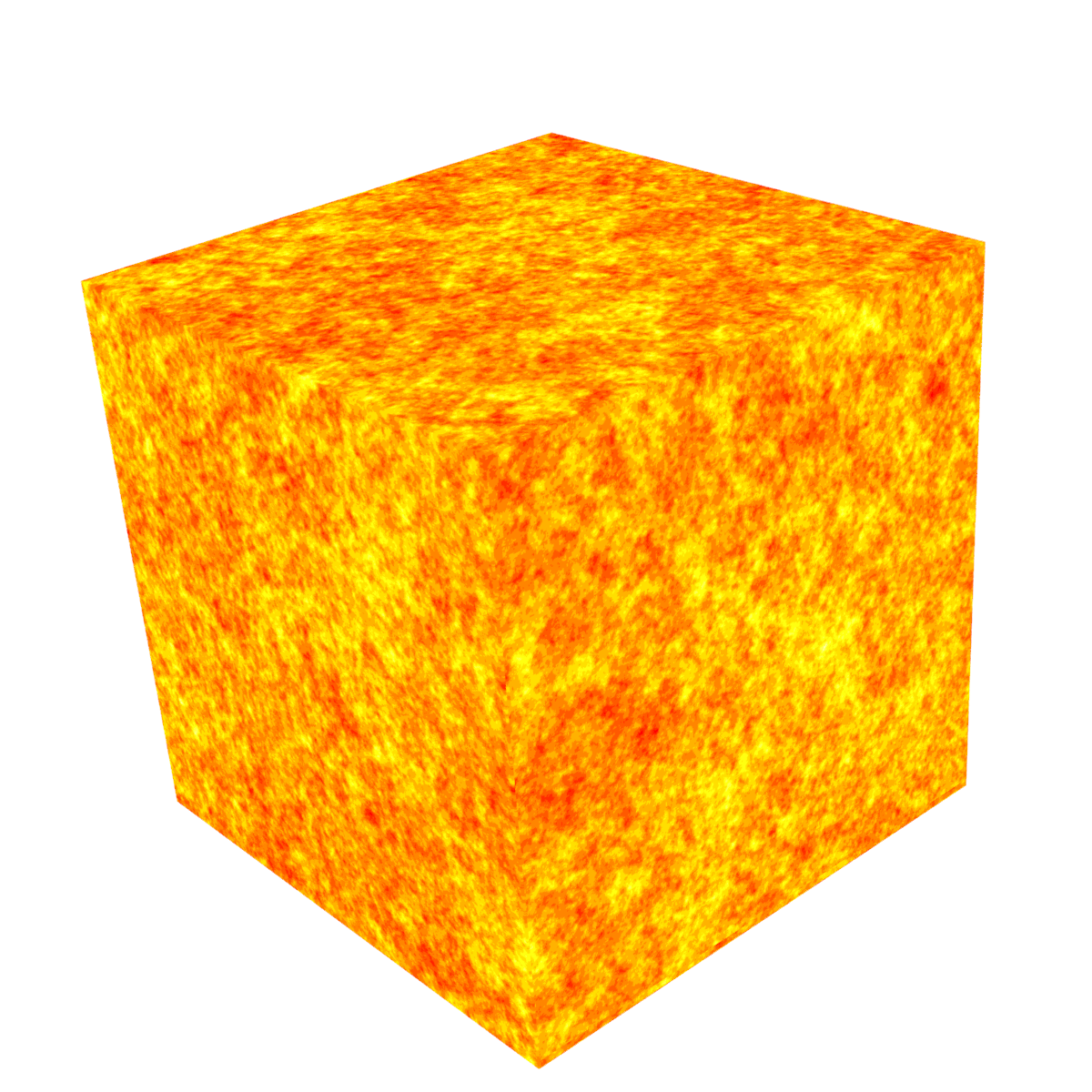
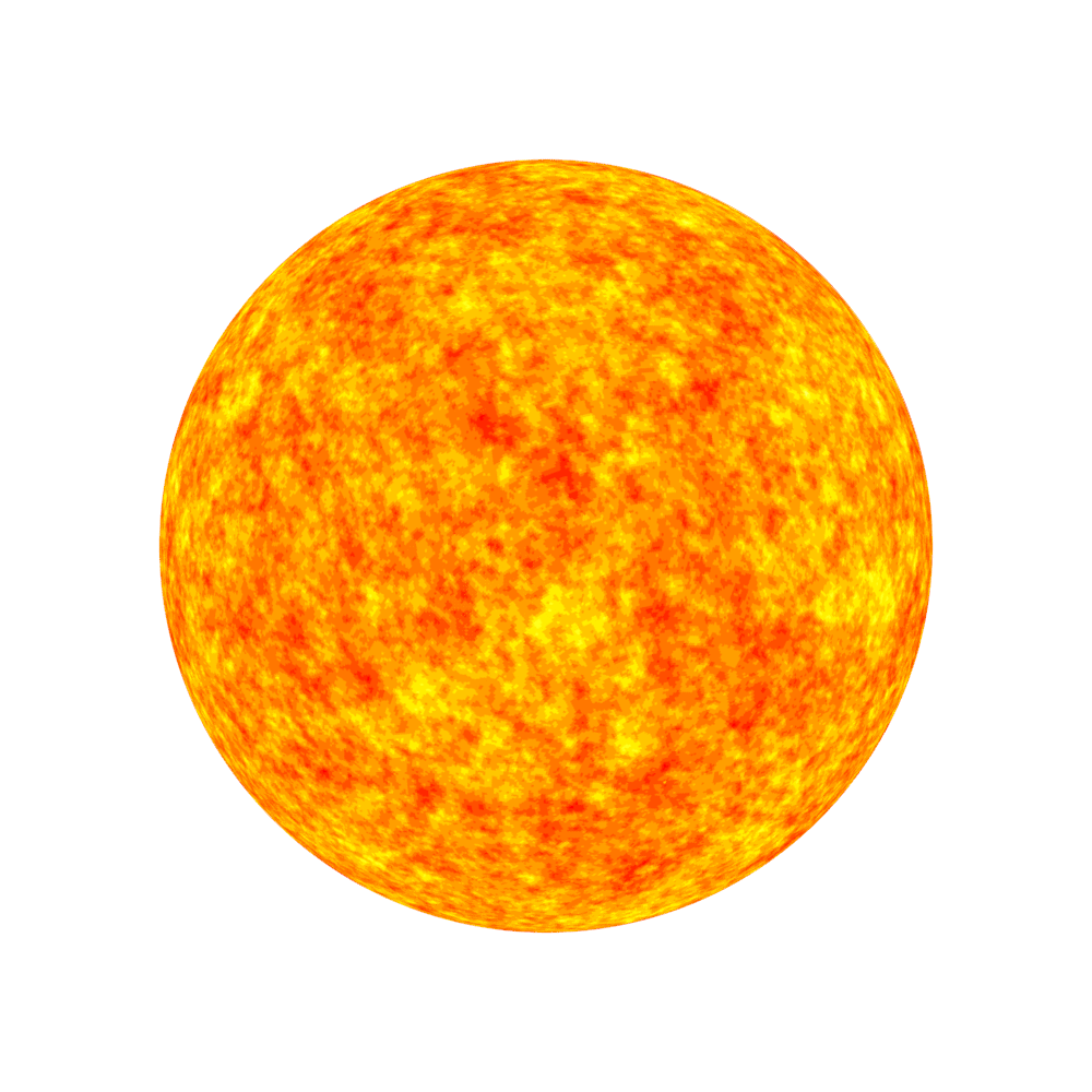
Random fields were simulated by using the R package ’RandomFields’, see [38]. Figure 1 provides two examples of the simulated Cauchy random field that were obtained.
Refer to caption
Refer to caption
Figure 1: Realizations of Cauchy random fields with α=23𝛼23\alpha=\frac{2}{3} on the sphere and the surface of the cube.

To verify the results of Sections 3 and 4 we simulated the random variables

Xr,G=κ!c2κ/2(d,α)Cκrd1κα2Lcκ2(r)|S(r)||P(r)|pP(r)G(η(p))hsp(pp),r[rmin,rmax],formulae-sequencesubscript𝑋𝑟𝐺𝜅superscriptsubscript𝑐2𝜅2𝑑𝛼subscript𝐶𝜅superscript𝑟𝑑1𝜅𝛼2superscriptsubscript𝐿𝑐𝜅2𝑟𝑆𝑟𝑃𝑟subscript𝑝𝑃𝑟𝐺𝜂𝑝subscript𝑠𝑝𝑝norm𝑝𝑟subscript𝑟𝑚𝑖𝑛subscript𝑟𝑚𝑎𝑥X_{r,G}=\frac{\kappa!c_{2}^{-\kappa/2}(d,\alpha)}{C_{\kappa}r^{d-1-\frac{\kappa\alpha}{2}}L_{c}^{\frac{\kappa}{2}}(r)}\frac{|S(r)|}{|P(r)|}\sum\limits_{p\in P(r)}G(\eta(p))h_{sp}\left(\frac{p}{\|p\|}\right),\,r\in[r_{min},r_{max}], (12)

where P(r):={pS(r)}assign𝑃𝑟𝑝𝑆𝑟P(r):=\{p\in S(r)\} is a discrete set of uniformly distributed points in S(r)𝑆𝑟S(r), |S()|𝑆|S(\cdot)| is the surface area of the sphere, |P()|𝑃|P(\cdot)| is the number of points in the set P()𝑃P(\cdot), and rminsubscript𝑟𝑚𝑖𝑛r_{min}, rmaxsubscript𝑟𝑚𝑎𝑥r_{max} denote the minimum and maximum values of the considered radius.

For the limit random variable Xκsubscript𝑋𝜅X_{\kappa} we considered the random variable XR,Gsubscript𝑋𝑅𝐺X_{R,G}, where R>>rmaxmuch-greater-than𝑅subscript𝑟𝑚𝑎𝑥R>>r_{max}.

Let d=3𝑑3d=3, α=2/3𝛼23\alpha=2/3, G(y)=H2(y)=y21𝐺𝑦subscript𝐻2𝑦superscript𝑦21G(y)=H_{2}(y)=y^{2}-1, rmin=200subscript𝑟𝑚𝑖𝑛200r_{min}=200, and rmax=3000subscript𝑟𝑚𝑎𝑥3000r_{max}=3000. Then the variables in (12) take the form

Xr,2=π3/2Γ(13)27/6r1/6K76(1/r)|S(r)||P(r)|pP(r)((η(p))21)hsp(pp),r[200,3000].formulae-sequencesubscript𝑋𝑟2superscript𝜋32Γ13superscript276superscript𝑟16subscript𝐾761𝑟𝑆𝑟𝑃𝑟subscript𝑝𝑃𝑟superscript𝜂𝑝21subscript𝑠𝑝𝑝norm𝑝𝑟2003000X_{r,2}=\frac{\pi^{3/2}\Gamma\left(\frac{1}{3}\right)}{2^{7/6}r^{1/{6}}K_{\frac{7}{6}}(1/r)}\frac{|S(r)|}{|P(r)|}\sum\limits_{p\in P(r)}((\eta(p))^{2}-1)h_{sp}\left(\frac{p}{\|p\|}\right),\,r\in[200,3000]. (13)

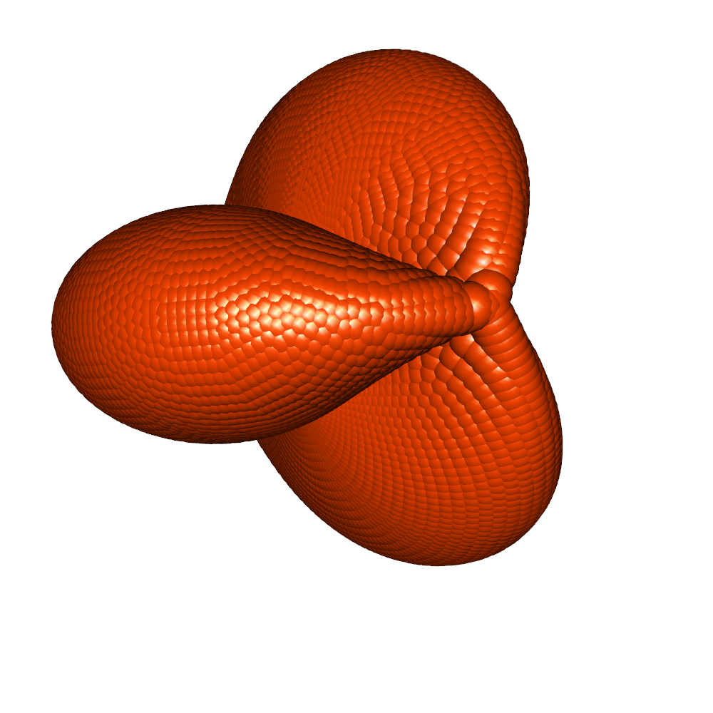
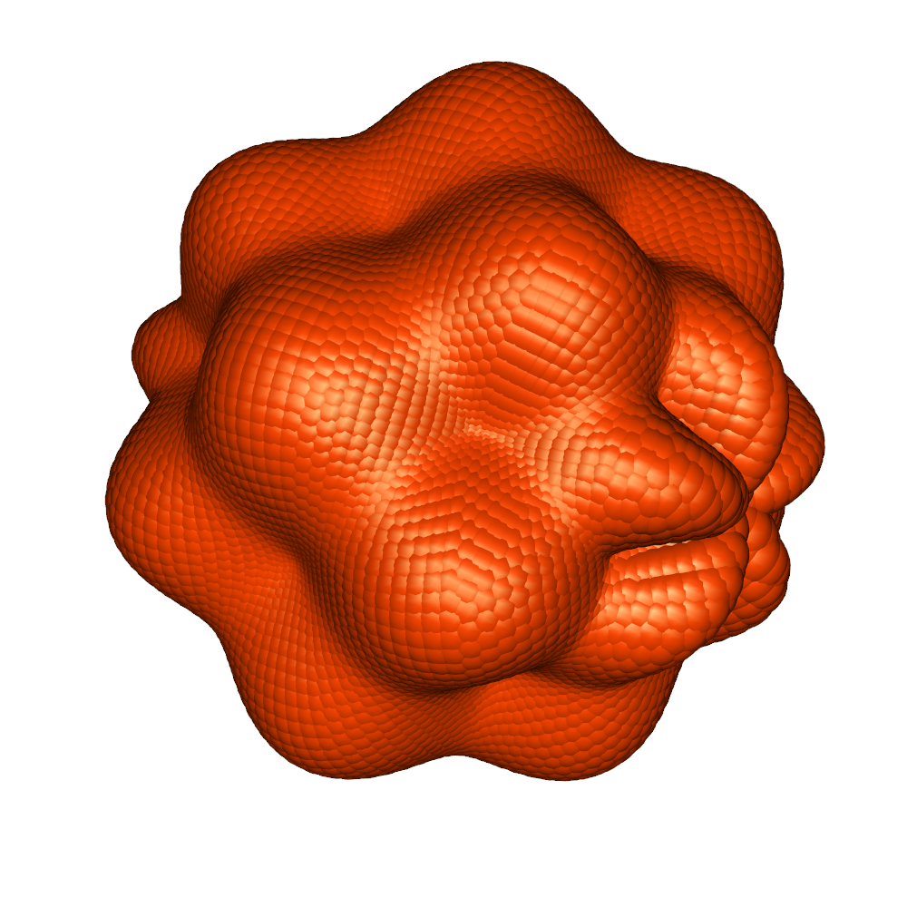
Let hsps(θ,ϕ):=1.2+0.2sin(5θ)sin(5ϕ)assignsuperscriptsubscript𝑠𝑝𝑠𝜃italic-ϕ1.20.25𝜃5italic-ϕh_{sp}^{s}(\theta,\phi):=1.2+0.2\sin(5\theta)\sin(5\phi) and hspc(θ,ϕ):=2+cos(3θ)assignsuperscriptsubscript𝑠𝑝𝑐𝜃italic-ϕ23𝜃h_{sp}^{c}(\theta,\phi):=2+\cos(3\theta), where θ𝜃\theta and ϕitalic-ϕ\phi are spherical coordinates. These functions embed the sphere of radius 1 and smoothly vary in different directions. We present two examples where we used hsps()superscriptsubscript𝑠𝑝𝑠h_{sp}^{s}(\cdot) as a weighted function in the case of spheres and hspc()superscriptsubscript𝑠𝑝𝑐h_{sp}^{c}(\cdot) as a weighted function in the case of cubes. See Figure 2 for the visualization of these functions.
Refer to caption
Refer to caption
Figure 2: Weighted functions hspssuperscriptsubscript𝑠𝑝𝑠h_{sp}^{s} (left) and hspcsuperscriptsubscript𝑠𝑝𝑐h_{sp}^{c} (right) used in the simulations.

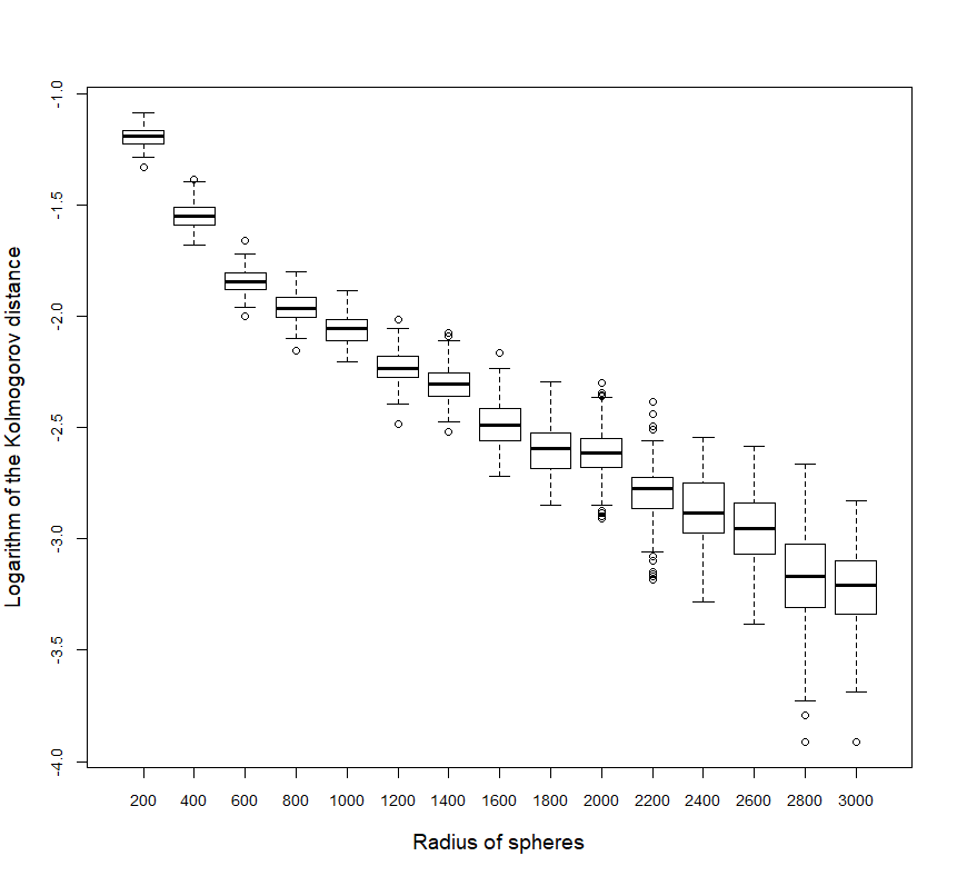
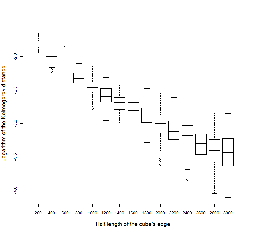
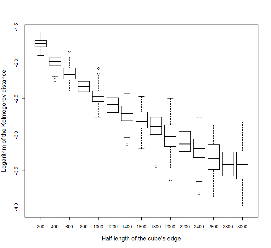
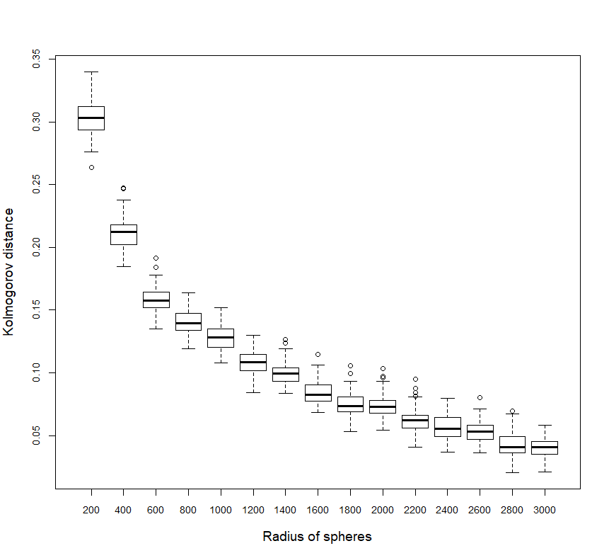
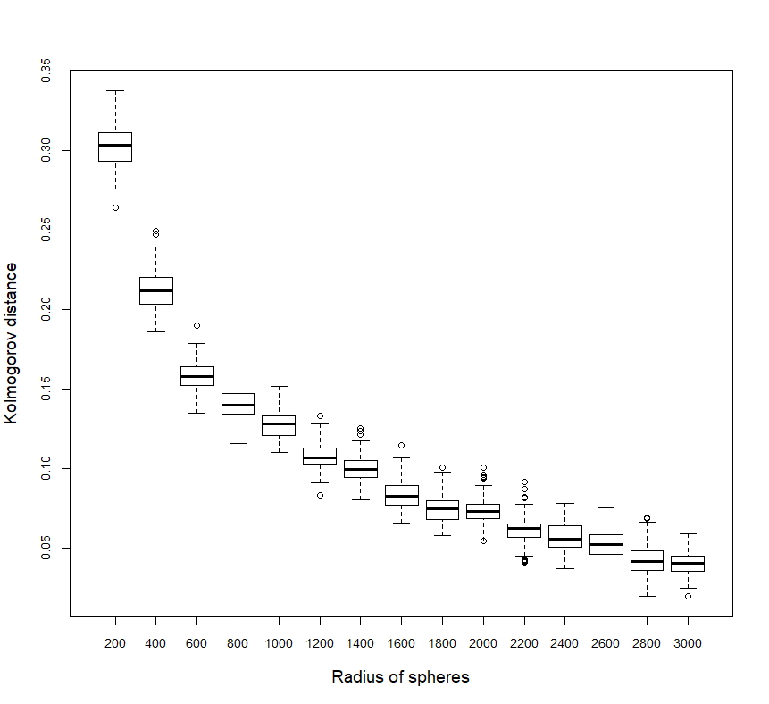
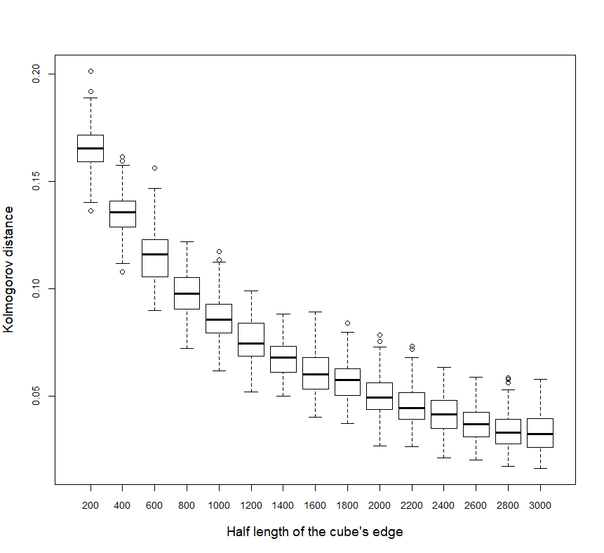
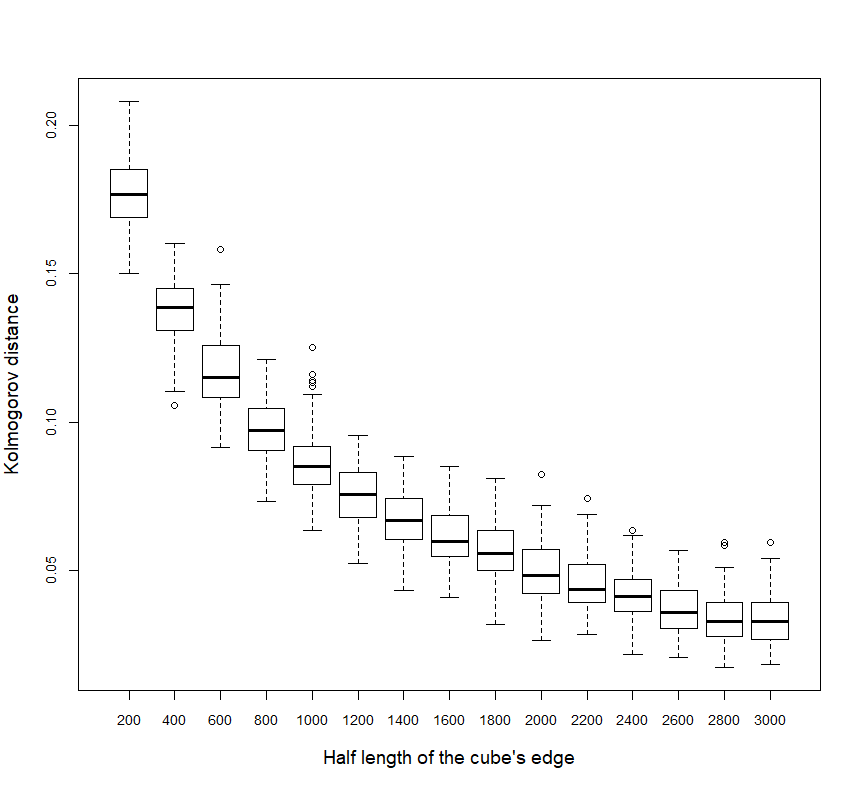
The sets P(r),r>0𝑃𝑟𝑟0P(r),\,r>0, were created by using the algorithm in [39] and setting the number of points |P(r)|r2similar-to𝑃𝑟superscript𝑟2|P(r)|\sim r^{2}. The random field η()𝜂\eta(\cdot) was simulated at the points P(r),r[200,3000],𝑃𝑟𝑟2003000P(r),r\in[200,3000], and at the points P(R)𝑃𝑅P(R). Each random variable (13) was simulated 2000 times. Using the simulated values, the Kolmogorov distance between Xr,2subscript𝑋𝑟2X_{r,2} and XR,2subscript𝑋𝑅2X_{R,2} was computed by the default Kolmogorov-Smirnov function ’ks.test’ in R. We present the results in two figures, obtained by repeating the simulation steps above 100 times. The first figure shows the box plots of the distances between Xr,2subscript𝑋𝑟2X_{r,2} and XR,2subscript𝑋𝑅2X_{R,2}. The second figure shows the corresponding box plots of the distance’s logarithms. The first figure displays actual convergence of the Kolmogorov distance for increasing r𝑟r. The second figure displays the changes in the power index of the rate of convergence.

For R=4000𝑅4000R=4000 and hsp()1subscript𝑠𝑝1h_{sp}(\cdot)\equiv 1 Figure 3 presents the obtained results for the unweighted case on spheres.
Refer to caption
Refer to caption
Figure 3: Simulation results for spheres with R=4000𝑅4000R=4000 and hsp()1subscript𝑠𝑝1h_{sp}(\cdot)\equiv 1.

In the weighted case hsp()=hsps()subscript𝑠𝑝superscriptsubscript𝑠𝑝𝑠h_{sp}(\cdot)=h_{sp}^{s}(\cdot) the obtained results are presented in Figure 4.
Refer to caption
Refer to caption
Figure 4: Simulation results for spheres with R=4000𝑅4000R=4000 and hsp()=hsps()subscript𝑠𝑝superscriptsubscript𝑠𝑝𝑠h_{sp}(\cdot)=h_{sp}^{s}(\cdot).

As one can see, Figures 3 and 4 are quite similar which indicates that un-weighted and weighted functionals have the same rate of convergence. This observation agrees with Theorem 4 according to which the weighted function has no effect on the rate of convergence. If the upper bound for the convergence rate in Theorem 4 was sharp, one would expect to see the means of Kolmogorov distance’s logarithms converge to a fixed value. Instead, we can see that the means form a declining slope, which might suggest that the real rate of convergence is a power function of the radius r𝑟r. By fitting the linear regression model we obtained the equation

log(ρ(Xr,2,XR,2))1.5120.000576r𝜌subscript𝑋𝑟2subscript𝑋𝑅21.5120.000576𝑟\log(\rho\left(X_{r,2},X_{R,2}\right))\approx-1.512-0.000576r (14)

in the unweighted case and a very similar equation in the weighted case.

Similar simulations were also conducted for cube surfaces. We considered 3-dimensional cube surfaces SQ(r)𝑆𝑄𝑟SQ(r) with the centre at the origin and the side lengths 2r,r>02𝑟𝑟02r,\,r>0. Thus, in (13) we replaced S(r)𝑆𝑟S(r) by SQ(r)𝑆𝑄𝑟SQ(r) and P(r)𝑃𝑟P(r) by PQ(r):={pSQ(r)}assign𝑃𝑄𝑟𝑝𝑆𝑄𝑟PQ(r):=\{p\in SQ(r)\}. Each PQ(r)𝑃𝑄𝑟PQ(r) was set by creating the equidistant grid for each side of the cube and, therefore, |PQ(r)|r2similar-to𝑃𝑄𝑟superscript𝑟2\left|PQ(r)\right|\sim r^{2}. To approximate integrals (5) by sums (12) with the equal precision in both sphere and cube cases we created approximately 6/π6𝜋6/\pi times more points on cubes than on spheres of the same radius. Other steps remained unchanged.

In the unweighted case hsp()1subscript𝑠𝑝1h_{sp}(\cdot)\equiv 1 the obtained results for surfaces of cube are presented in Figure 5.
Refer to caption
Refer to caption
Figure 5: Simulation results for cubes with R=4000𝑅4000R=4000 and hsp()1subscript𝑠𝑝1h_{sp}(\cdot)\equiv 1.

In the weighted case hsp()=hspc()subscript𝑠𝑝superscriptsubscript𝑠𝑝𝑐h_{sp}(\cdot)=h_{sp}^{c}(\cdot) we obtained the results presented in Figure 6.
Refer to caption
Refer to caption
Figure 6: Simulation results for cubes with R=4000𝑅4000R=4000 and hsp()=hspc()subscript𝑠𝑝superscriptsubscript𝑠𝑝𝑐h_{sp}(\cdot)=h_{sp}^{c}(\cdot).

As one can see, in the case of cubes the rate of convergence is also similar in both weighted and unweighted cases. Furthermore, these figures also suggest a power rate of convergence. By fitting the linear regression lines we obtained the equation log(ρ(Xr,2,XR,2))1.830.000571r𝜌subscript𝑋𝑟2subscript𝑋𝑅21.830.000571𝑟\log(\rho\left(X_{r,2},X_{R,2}\right))\approx-1.83-0.000571r in the unweighted case and the equation log(ρ(Xr,2,XR,2))1.810.000584r𝜌subscript𝑋𝑟2subscript𝑋𝑅21.810.000584𝑟\log(\rho\left(X_{r,2},X_{R,2}\right))\approx-1.81-0.000584r in the weighted case. The slopes of these equations are very similar to the slope in (14), indicating the same rate of convergence in the cases of both surfaces.

6 Directions for future research

This paper discussed the asymptotic behaviour of least squares estimators in regression models for long-range dependent random fields observed on spheres. The results were obtained under rather general assumptions on the random fields.

We expect that the results derived in Sections 3 and 4 also hold in the case of random fields observed on more general surfaces. This conjecture is supported by the results in Section 5, where asymptotic behaviour of LSE was studied for the cases of sphere and cube surfaces. The obtained results were quite similar in both cases.

The upper bound for the rate of convergence presented in the paper is the first result of such type for LSE. It would be interesting to obtain sharp upper bounds and extremal examples. The results of Section 5 suggest that the actual speed of convergence of LSE might be a power function of r𝑟r.

The linear regression model was considered in this paper. It would be interesting to obtain analogous results for non-linear regression models.

Acknowledgements

This research was partially supported under the Australian Research Council’s Discovery Project DP160101366.
This research includes extensive simulation studies using the computational cluster Raijin of the National Computational Infrastructure (NCI), which is supported by the Australian Government and La Trobe University.

References

  • [1] Ruiz-Medina M. New challenges in spatial and spatiotemporal functional statistics for high-dimensional data. Spat Stat. 2012;1:82–91.
  • [2] Ivanov A, Leonenko N, Ruiz-Medina M, et al. Estimation of harmonic component in regression with cyclically dependent errors. Statistics. 2015;49(1):156–186.
  • [3] Louhichi S, Miura R, Volný D. On the asymptotic normality of the R-estimators of the slope parameters of simple linear regression models with associated errors. Statistics. 2017;51(1):167–187.
  • [4] Doyen PM. Porosity from seismic data: A geostatistical approach. Geophysics. 1988;53(10):1263–1275.
  • [5] Yadrenko MI. Spectral theory of random fields. New York (NY): Optimization Software; 1983.
  • [6] Ivanov AV, Leonenko NN, Ruiz-Medina MD, et al. Limit theorems for weighted nonlinear transformations of Gaussian stationary processes with singular spectra. Ann Probab. 2013;41(2):1088–1114.
  • [7] Cohen G, Francos JM. Linear least squares estimation of regression models for two-dimensional random fields. J Multivar Anal. 2002;82(2):431–444.
  • [8] De Oliveira V, Kedem B, Short DA. Bayesian prediction of transformed Gaussian random fields. J Am Stat Assoc. 1997;92(440):1422–1433.
  • [9] Vio R, Andreani P, Wamsteker W. Numerical simulation of non-Gaussian random fields with prescribed correlation structure. PASP. 2001;113(786):1009–1020.
  • [10] Frias M, Alonso F, Ruiz-Medina M, et al. Semiparametric estimation of spatial long-range dependence. J Stat Plan Inference. 2008;138(5):1479–1495.
  • [11] Doukhan P, Oppenheim G, Taqqu M. Long-range dependence: Theory and applications. Boston (MA): Birkhäuser; 2003.
  • [12] Ivanov AV, Leonenko NN. Statistical analysis of random fields. Dordrecht: Springer; 1989.
  • [13] Wackernagel H. Multivariate geostatistics. Berlin: Springer; 1998.
  • [14] Guinness J, Fuentes M. Isotropic covariance functions on spheres: Some properties and modeling considerations. J Multivar Anal. 2016;143:143–152.
  • [15] Leonenko N, Ruiz-Medina M. Increasing domain asymptotics for the first Minkowski functional of spherical random fields. Theory Probab Math Stat. 2017;97:120–141.
  • [16] Marinucci D, Peccati G. Random fields on the sphere: representation, limit theorems and cosmological applications. New York (NY): Cambridge University Press; 2011.
  • [17] Leonenko N, Yadrenko M, Il’icheva L. On the efficiency of the least squares estimator of regression coefficients of a random field observed on a sphere. In: Exploring stochastic laws. Utrecht; 1995. p. 257–262.
  • [18] Olenko A, Vaskovych V. Non-central limit theorems for functionals of random fields on hypersurfaces; 2018. arXiv:1810.09285.
  • [19] Leonenko N, Taufer E. Asymptotic properties of LSE in multivariate continuous regression with long memory stationary errors. Metron. 2001;59(1–2):55–72.
  • [20] Dobrushin RL, Major P. Non-central limit theorems for non-linear functional of Gaussian fields. Z Wahrsch Verw Gebiete. 1979;50(1):27–52.
  • [21] Taqqu MS. Weak convergence to fractional Brownian motion and to the Rosenblatt process. Z Wahrsch Verw Gebiete. 1975;31(4):287–302.
  • [22] Taqqu MS. Convergence of integrated processes of arbitrary Hermite rank. Z Wahrsch Verw Gebiete. 1979;50(1):53–83.
  • [23] Anh V, Leonenko N, Olenko A, et al. On rate of convergence in non-central limit theorems; 2018. Bernoulli, Forthcoming; arXiv:1703.05900.
  • [24] Olenko A. Limit theorems for weighted functionals of cyclical long-range dependent random fields. Stoch Anal Appl. 2013;31(2):199–213.
  • [25] Peccati G, Taqqu MS. Wiener chaos: Moments, cumulants and diagrams: A survey with computer implementation. Milano: Springer; 2011.
  • [26] Bingham NH, Goldie CM, Teugels JL. Regular variation. New York (NY): Cambridge University Press; 1989.
  • [27] Petrov VV. Limit theorems of probability theory: sequences of independent random variables. New York (NY): Oxford University Press; 1995.
  • [28] Leonenko N, Olenko A. Tauberian and Abelian theorems for long-range dependent random fields. Methodol Comput Appl Probab. 2013;15(4):715–742.
  • [29] Itô K. Multiple Wiener integral. J Math Soc Japan. 1951;3(1):157–169.
  • [30] Major P. Multiple Wiener-Itô integrals. Berlin: Springer; 1981.
  • [31] Seneta E. Regularly varying functions. Berlin: Springer; 1976.
  • [32] Iosevich A, Liflyand E. Decay of the Fourier transform. Basel: Birkhäuser; 2014.
  • [33] Stein EM. Beijing lectures in harmonic analysis. Princeton (NJ): Princeton University Press; 2016.
  • [34] Leonenko N. Limit theorems for random fields with singular spectrum. Dordrecht: Springer; 1999.
  • [35] Alodat T, Olenko A. Weak convergence of weighted additive functionals of long-range dependent fields. Theory Probab Math Statist. 2017;97:9–23.
  • [36] Donoghue W. Distributions and Fourier transforms. New York (NY): Academic Press; 1969.
  • [37] Olver FW, Lozier DW, Boisvert RF, et al. NIST handbook of mathematical functions. New York (NY): Cambridge University Press; 2010.
  • [38] Schlather M, Malinowski A, Menck PJ, et al. Analysis, simulation and prediction of multivariate random fields with package RandomFields. J Stat Softw. 2015;63(8):1–25.
  • [39] Deserno M. How to generate equidistributed points on the surface of a sphere. P-If Polymerforshung (Ed). 2004;Available from: https://www.cmu.edu/biolphys/deserno/pdf/sphere$_$equi.pdf.