Enhancing Domain Word Embedding via Latent Semantic Imputation
Abstract.
We present a novel method named Latent Semantic Imputation (LSI) to transfer external knowledge into semantic space for enhancing word embedding. The method integrates graph theory to extract the latent manifold structure of the entities in the affinity space and leverages non-negative least squares with standard simplex constraints and power iteration method to derive spectral embeddings. It provides an effective and efficient approach to combining entity representations defined in different Euclidean spaces. Specifically, our approach generates and imputes reliable embedding vectors for low-frequency words in the semantic space and benefits downstream language tasks that depend on word embedding. We conduct comprehensive experiments on a carefully designed classification problem and language modeling and demonstrate the superiority of the enhanced embedding via LSI over several well-known benchmark embeddings. We also confirm the consistency of the results under different parameter settings of our method.
1. Introduction
Embedding words and phrases in continuous semantic spaces has a significant impact on many natural language processing (NLP) tasks. There are two main types of word embedding approaches aiming at mapping words to real-valued vectors: matrix factorization (Deerwester et al., 1990; Lund and Burgess, 1996; Pennington et al., 2014) and neural networks (Bengio et al., 2003; Mikolov et al., 2013b). The embedding matrix is a reflection of the relative positions of words and phrases in semantic spaces. Embedding vectors pre-trained on large corpora can serve as the embedding layer in neural network models and may significantly benefit downstream language tasks because reliable external information is transferred from large corpora to those specific tasks.
Word embedding techniques have achieved remarkable successes in recent years. Nonetheless, there are still critical questions that are not well answered in the literature. For example, considering that word embedding usually relies on the distributional hypothesis (Harris, 1954), it is difficult to generate reliable word embeddings if the corpus size is small or if indispensable words have relatively low frequencies (Bojanowski et al., 2016). Such cases can happen in various domain-specific language tasks, e.g., chemistry, biology, and healthcare, where thousands of domain-specific terminologies exist. This challenge naturally drives us to find an effective way to leverage available useful information sources to enhance the embedding vectors of words and phrases in domain-specific NLP tasks. From the perspective of linear algebra, the problem falls into the scope of combining two matrices, both of which describe entities in their own spaces. Theoretically, the combination task can be addressed even if the two matrices do not have identical dimensions; however, the sets of entities they describe must have an intersection to be combined.
In this paper, we propose a novel method, named Latent Semantic Imputation, to combine representation matrices, even those representation matrices defined in different Euclidean spaces. The framework can be further adapted to address the problem of unreliable word embedding and to effectively and efficiently transfer domain affinity knowledge to semantic spaces or even from one semantic space to another. The knowledge transfer becomes the indispensable strategy to fundamental NLP tasks and ultimately improves their performance. In summary, the contributions of this paper are as follows:
-
•
We formalize the problem of combining entity representations in different Euclidean spaces and propose the method of Latent Semantic Imputation (LSI111Code available at https://github.com/ShiboYao/LatentSemanticImputation) to solve the problem.
-
•
To ensure the deterministic convergence, we propose a minimum spanning tree -nearest neighbor graph (MST--NN) and seek a sparse weight matrix via solving non-negative least squares problems with standard simplex constraints. Such a sparse weight matrix is a representation of the latent manifold structure of the data.
-
•
We design a power iteration method that depicts a random walk on a graph to derive the unknown word embedding vectors while preserving the existing embeddings.
-
•
We demonstrate how LSI can be further adapted for enhancing word embedding and will benefit downstream language tasks through experiments.
2. Related Work
A typical matrix factorization approach for word embedding is based on word co-occurrence matrices. Such a matrix implicitly defines a graph in which the vertices represent words and the matrix itself encodes the affinity. By taking a set of significant eigenvectors of this matrix, we attain low-dimensional word embedding, with a couple of variations (Bullinaria and Levy, 2007; Turney and Pantel, 2010; Deerwester et al., 1990; Hashimoto et al., 2016; Levy and Goldberg, 2014; Lund and Burgess, 1996). The neural network approach for word embedding dates back to the neural probabilistic language model (Bengio et al., 2003), where the embeddings are precisely the weight matrix of the first hidden layer and generated during the language model training process. The common practice nowadays is to put the embeddings pre-trained from a large corpus back into the embedding layer of the neural network and facilitate the training of language tasks. These two approaches appear to be isolated from each other; nevertheless, they have surprisingly fundamental connections. Levy and Goldberg illustrated that skip-gram with negative sampling (SGNS) (Mikolov et al., 2013b) implicitly factorizes the word-context matrix constructed from the point-wise mutual information (Levy and Goldberg, 2014). Li et al. (2015) argued that SGNS is an explicit factorization of the word co-occurrence matrices. From the perspective of vector space models of semantics (Turney and Pantel, 2010), the log co-occurrence of words is related to their semantic similarity, and the word embedding method is a metric recovery process in semantic spaces with manifold learning (Hashimoto et al., 2016).
Our study is closely related to spectral embedding methods that try to calculate the most significant eigenvectors (or linear combinations of the significant eigenvectors) of the adjacency matrix. The idea of spectral embedding methods dates back to principal component analysis (Diamantaras and Kung, 1996) that is widely used for linear dimensionality reduction. With the Laplacian matrix, spectral embedding methods capture the nonlinearity and expand its application cases into clustering (Von Luxburg, 2007; Lin and Cohen, 2010; Huang et al., 2014) and nonlinear dimensionality reduction.
The construction of the weight matrix (or affinity matrix) is essential in spectral embedding. The weight matrices are usually sparse due to the assumption that data points in Euclidean spaces only “interact” with their nearest neighbors and reveal the Euclidean geometrical properties locally (Saul and Roweis, 2003). In other words, the high-dimensional data usually follow a lower-dimensional manifold distribution (Roweis and Saul, 2000). Manifold learning has a wide range of applications in representation learning and data visualization (Belkin and Niyogi, 2003; Maaten and Hinton, 2008). Manifold learning has an intrinsic relationship with graph theory due to the common practice of using graphs to describe the manifold structure embedded in the original high-dimensional space (Roweis and Saul, 2000; Liu et al., 2010).
Manifold learning models often produce closed-form solutions. However, closed-form solutions usually involve the inverse or eigendecomposition of a large matrix, both of which are computationally expensive. Instead, we leverage the power iteration method to obtain solutions efficiently in the case where the primary concern is the time complexity. This work is also inspired by transductive learning and label propagation (Zhu and Ghahramani, 2002; Bengio et al., 2006). The major difference is that label propagation tries to propagate labels in the label space, while our work seeks to learn representations in the semantic space. For the power iteration to converge deterministically, that is, where the final result does not depend on the initialization of the unknown embeddings, we have to rigorously formulate the processes of constructing the graph and solving its weight matrix.
3. Problem Definition and Proposed Approach Overview
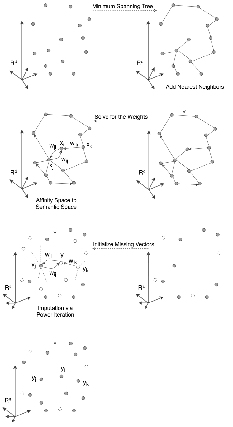
stands for -dimensional affinity space, stands for -dimensional semantic space.
The state-of-the-art word embedding methods adopt a common practice of neglecting low-frequency words before training in order to minimize the effect of low-frequency words and ensure reliable results (Mikolov et al., 2013b)(Pennington et al., 2014). However, neither excluding these words with nor indiscriminately including them in the vocabulary works well because the valuable information of low-frequency words should be preserved for domain-specific language tasks. For example, thousands of company names in financial news analysis, disease and medicine abbreviations in health-care problems, and functional and radical groups in chemistry. Sometimes, it is also desired to expand the vocabulary of word embedding to minimize the effect of out-of-vocabulary words. To quantify such problems, we may combine different embedding matrices or fuse data from multiple sources and transfer prior knowledge into the semantic space to enhance the word embedding.
The underlying problem is to transfer entity representations from one Euclidean space to another. Suppose there is a set of entities with their representation vectors in space and a set of entities whose representation vectors are in space , where . We would like to approximate the entity representations of (entities exist in and not in ) in ’s representation space or approximate the entity representations of in space .
To further elaborate the mechanisms of Latent Semantic Imputation, we take the embedding of company names as an example. Some company names are relatively low-frequency words in corpora. Discarding these names will be a suboptimal choice since the names are likely to be essential for downstream language tasks. On the other hand, adding them to the dictionary might lead to unreliable word embedding results. We discovered that different types of information might be complementary to each other. For example, we can use the historical trading price of publicly listed companies or the financial features of companies to define another matrix that describes the entity similarity, other than the word embedding matrix. Thereby, we transfer the rich information from this domain matrix to the word embedding matrix. From the graph perspective, the graph defined by the domain matrix and the graph defined by the word embedding matrix often have similar topological structures. Therefore, we can apply the graph topology that is determined by the domain matrix to recover the local graph structure of the company names that are missing from the semantic space due to their low frequency. The domain matrix is determined by domain statistics and might vary according to the available data source; e.g., a domain matrix in chemistry is based on the co-occurrence of functional or radical groups in a basket of molecules, while one in healthcare is derived from the medicine or disease features.
To use Latent Semantic Imputation to enhance domain word embedding, we take the following steps: (1) Identify a reliable embedding matrix as the base. The embedding is trained with a large corpus, e.g., billions of words or gigabytes of plain text. (2) Identify or construct a domain matrix that describes the entities within the specific domain. (3) Apply latent semantic imputation to recover those embedding vectors that are not in the initial set of word embedding vectors.
4. Latent Semantic Imputation
We obtained inspiration from manifold learning (Belkin and Niyogi, 2003; Maaten and Hinton, 2008; Saul and Roweis, 2003), particularly one of the pioneering works, Locally Linear Embedding (LLE) (Roweis and Saul, 2000). Based on LLE, we argue that the words are in a lower-dimensional manifold embedded in the original high-dimensional space. A manifold is a topological space that locally resembles Euclidean space near each point, and therefore we need to think globally for the overall embedding context and fit locally for each single data point (Saul and Roweis, 2003).
We specifically denote the domain data matrix , where is the entity number and is the dimension, and use to represent the embedding matrix in the semantic space, where is the vocabulary size and is the dimension of the semantic space. Note that there are entities in the intersection of and . Without loss of generality, we permute the vectors to arrange the overlapping part to be the upper part of the two matrices. The bottom vectors in will be reconstructed into . The remaining vectors of that are outside of the overlapping part are irrelevant. They remain unchanged, do not contribute any information and will be directly fed into downstream language tasks. Hence we temporally discard them. Our goal is to find the missing vectors (or matrix ) in given the domain matrix and the known vectors () in the semantic space. For simplicity, we use where to denote a vertical concatenation of and , namely, the known embedding vectors and the missing embedding vectors in the semantic space. The whole process is essentially a data imputation.
| (1) |
where and are the vectors in the affinity space and the semantic space, respectively. We denote vectors with bold letters like in the following sections.
Latent Semantic Imputation consists of three steps:
Step 1. Build a minimum-spanning-tree -nearest neighbor graph given the domain matrix ,
Step 2. Solve for the sparse weight matrix using non-negative least squares with standard simplex constraints, and
Step 3. Recover the missing embedding vectors in the semantic space using the power iteration method.
4.1. The Minimum-Spanning-Tree -NN Graph
Locally Linear Embedding argues that a data point is a linear combination of its nearest neighbors under the manifold assumption (Roweis and Saul, 2000), which means , where if belongs to the nearest neighbors of and zero otherwise.
Building a -NN graph is the first step in LLE. However, it is not sufficient in Latent Semantic Imputation. To elaborate on this, we first notice that a -NN graph is not necessarily a connected graph and might contain some connected components with all vertices not having embedding vectors in the semantic space before imputation. In such cases, even if we have the topology derived from the domain matrix, these data points can still be arbitrarily shifted or rotated in the target semantic space because their mean and covariance are not constrained. These embedding results are obviously erroneous. In particular, the idea of Latent Semantic Imputation is to transfer the prior knowledge, in the format of a domain matrix extracted from other data sources, into the semantic space and impute those missing embedding vectors. The iterative process requires the graph being connected to propagate information, which is similar to the network flow (Ahlswede et al., 2000). In a disconnected graph, some of the embedding vectors form data cliques (isolated subgraphs), and the information is not able to propagate through different subgraphs.
On the contrary, it is desirable that the known embedding vectors serve as “anchors” (Liu et al., 2010) in the graph. In Figure 1, is a vector in the affinity space, and its corresponding embedding vector in the semantic space is . In the process of imputation, serves as an anchor to stabilize the positions of unknown word embedding vectors. To this end, we construct a Minimum-Spanning-Tree -Nearest-Neighbor (MST--NN) graph which ensures the connectivity to describe the topological structure of the entities in the affinity space. We will show in a later section that a MST--NN graph guarantees deterministic convergence in the power iteration. That is, the final results do not depend on the initialization of .
In the MST--NN graph construction, we first find a minimum spanning tree (Kruskal, 1956) based on the Euclidean distance matrix of entities given the domain matrix . In a minimum spanning tree, some nodes can be dominated by one or two neighbors, which would be likely to introduce bias and sensitivity. Therefore on top of the minimum spanning tree, we search for additional nearest neighbor(s) of each node and add directed edge(s) between these additional neighbor(s) and the corresponding node if the in-degree of the node is smaller than . After this step, the minimum degree of the graph is (previously, some vertices in the minimum spanning tree can have a degree larger than ), and we denote this hyperparameter . In practice, we did not find it necessary to add degree constraints because the graph construction usually preserves the manifold assumption. In other words, the maximum node degree in the minimum spanning tree usually does not exceed or not exceed significantly.
Note that the graph from the minimum spanning tree is un-directed (symmetric adjacency matrix, or two nodes are mutually reachable if they have an edge), while the graph after the nearest neighbor search is directed because the nearest neighbor relationship is not communicative.
4.2. Non-Negative-Least-Squares to Solve
The second step of Latent Semantic Imputation is to resolve the optimal weights. In this step, we explicitly impose two constraints on the weights: being non-negative and normalized. These two constraints jointly define a standard simplex constraint to the least squares problem. Solving such problems produces a random walk matrix where the weight values are bounded by and and all row sums are . Such matrices have the desired property that the absolute eigenvalues have the upper-bound because the dominant eigenvalue modulus is bounded by the smallest and largest row sums(Seneta, 2006), both of which are . The objective function for solving the weight matrix in the affinity space is
| (2) | ||||||
| s.t. | ||||||
To solve this problem, note that it can be reduced to non-negative least squares problems each of which tries to solve for an optimal weight vector with the same constraints, since solving for weight vector has no influence on solving for , .
Lawson and Hanson first proposed the active set method to solve non-negative least squares problems (Lawson and Hanson, 1995). Once the non-negative weight vectors are obtained (Jones et al., 2014), they will be normalized. Note that the weight matrix is sparse due to the manifold assumption. Furthermore, all column vectors because the graph generated from the MST step is connected.
4.3. Power Iteration Method to Solve Matrix
Our algorithm rests upon the assumption that the local structures are similar to each other between the affinity space and the semantic space, defined by the sparse weight matrix . Based on this assumption, we design a mapping that preserves the local structures embedded in the two different spaces, fixes the known embedding vectors and lets adapt to the affinity information. In this setting, imposes additional constraints on the optimization problem. Based on the findings in transductive learning and label propagation (Zhu and Ghahramani, 2002; Bengio et al., 2006), the power iteration method is suitable for the imputation problem. The final embedding vectors are a series of linear combinations of the dominant eigenvectors of the weight matrix. We denote the lower rows of the weight matrix as and the time step , and apply the following iterative process to solve for :
| (3) |
4.3.1. Spectral Radius of a Square Matrix
The spectral radius of a square matrix is its largest absolute eigenvalue
According to the Perron-Frobenius theorem, the eigenvalue modulo of retrieved from step is bounded by (Seneta, 2006). To expand on this, first note that the non-negative weight matrix is irreducible because its associated graph is a strongly connected graph(Seneta, 2006) that is constructed from a minimum spanning tree. Therefore, is bounded by its maximal and minimal row sums,
| (4) |
The row sum of is always as a result of the normalization in solving . Hence, the spectral radius . In fact, the dominant eigenvalue is and unique. This ensures convergence in the power iteration. To fix the known embeddings , we set to identity, which results in eigenvalues being and the rest having a modulo strictly smaller than .
4.3.2. Power Method for Eigenvectors
The power method is often used for calculating the eigenvectors of a given square matrix . Given a random vector , the power method iteratively multiplies the vector by matrix and divides the product by its norm . The embedding vector eventually becomes the dominant eigenvector of matrix . In our case, suppose we have a random vector that is a linear combination of ’s eigenvectors (at this moment, is not changed to identity and has a unique dominant eigenvalue), , where is the weight of the dominant eigenvector and is usually nonzero. There exists an eigengap between the dominant eigenvalue and the rest, , and consequently, the weights of the non-dominant eigenvectors shrink rapidly and eventually become zero after a certain number of iterations. eventually becomes the dominant eigenvector of :
and thus, In our case, the initial weights of the dominant eigenvectors are in fact determined by the known embedding vectors.
4.3.3. Implementation Details
In practice, is fixed, and only needs to be updated during the iteration. Therefore, we set to identity,
| (5) |
and then apply the power iteration to update the embedding matrix: . Note that changing the upper rows to identity does not change the spectral radius of . The observation is derived from the characteristic equation of . In fact, there will be eigenvectors associated with eigenvalue after this step, guaranteeing that the final embedding matrix is filled with linear combinations of ’s dominant eigenvectors whose weights are determined by the initial coefficients that are solely determined by .
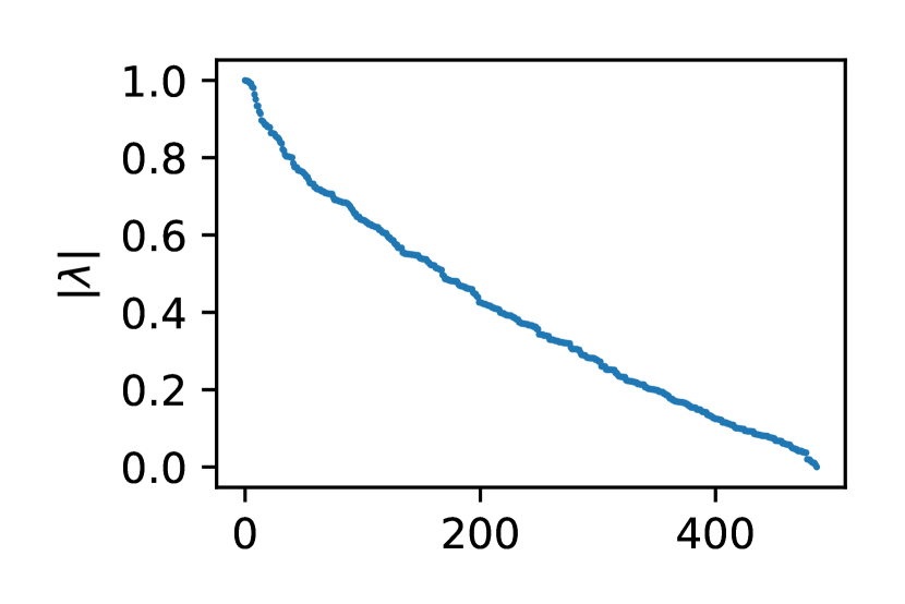
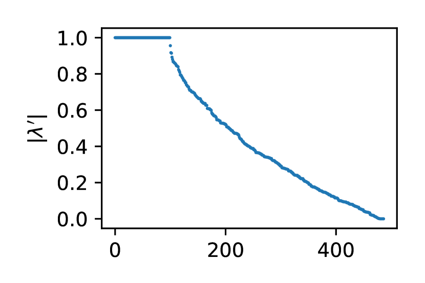
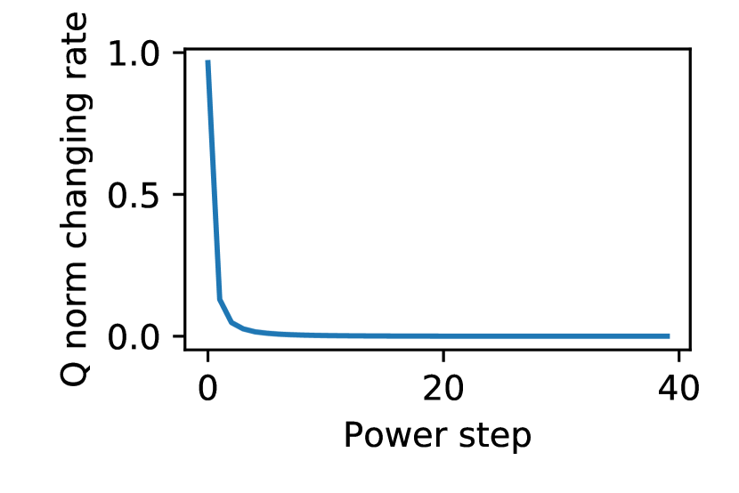
The stopping criterion is the convergence of when the -norm changing rate of between two iterations falls under a predefined threshold or when the maximum number of iterations is reached.
| (6) |
The computational complexity of the LSI depends on the size of the domain matrix. The Euclidean distance matrix calculation, -NN search and quadratic programming are embarrassingly paralleled. It takes less than a minute on a PC to perform LSI on a domain matrix with about 4k samples. The time complexity of building the Euclidean distance matrix is where is the dimension of the data space and is the sample number. The time complexity of building a minimum spanning tree is typically . It takes approximately to search for additional nearest neighbors for all nodes via partition, where (the sample number is equal to the number of vertices in the graph). LSI only takes a marginal time compared to the general word embedding algorithms that usually require hours or even days for training.
4.4. Deterministic Convergence of LSI
To better illustrate the convergence properties of LSI, we follow the logic in (Zhu and Ghahramani, 2002). From the graph perspective, in Eqn 5 means that the nodes in have self-loops ( is fixed); the upper right zero matrix indicates that there are no edges from to ( has no influence on ); represents the weighted edges from to (diffusion from to ); and represents the weighted edges within (diffusion within ). We show that LSI guarantees deterministic convergence regardless of the initialization of .
Theorem 4.1.
If is a convergent matrix, i.e., , then LSI guarantees deterministic convergence.
Proof.
Rewrite the power iteration as follows:
| (7) | |||
| (8) |
Given , the final embedding result is deterministic regardless of . ∎
Now we show that under our algorithm settings, is a convergent matrix. Note that is a substochastic matrix, i.e.,
. This is a result of the minimum spanning tree where there exists one edge from to (one positive value in ), and hence, there exists one row sum of strictly less than . In fact, under the MST--NN graph setting, there are many edges from to due to the additional nearest neighbor search. After all, these edges serve the major assumption of imputation and allow us to leverage the known embeddings for diffusion. Additionally, due to the minimum spanning tree step at the beginning, we have the following lemma:
Lemma 4.0.
For every node in , there always exists a path from to this node.
Definition 4.0 (Sink Node).
Let , the -th row sum. A sink node in a substochastic matrix is one with .
Given Lemma 4.2, we have the following corollary:
Corollary 4.0.0.
For every node in , either it is a sink node or there exists a path from a sink node to it, or both.
Lemma 4.0.
For a substochastic matrix, for every non-sink node, if there exists a path from a sink node to this non-sink node, then the substochastic matrix is convergent.
Proof.
To show , we need to show
or for a finite
For every sink node in , we have . And
Since we have ,
Thus, the convergence is apparently true for those sink nodes. Suppose the shortest path (with all positive edges) from a sink node to a non-sink node within has steps. Then, we have
and
Hence, the following condition holds:
Because our graphs are always finite, the convergence also holds for the non-sink nodes. ∎
5. Experiments
We applied two types of evaluation methods for word embedding: intrinsic evaluation and extrinsic evaluation (Schnabel et al., 2015), to validate LSI. Categorization is an intrinsic evaluation in which word embedding vectors are clustered into different categories. Clustering is also one of the principles for designing the hierarchical softmax word embedding model (Mnih and Hinton, 2009). The extrinsic evaluation involves downstream language tasks. In our experiments, we used the -NN classifier on a group of embedding vectors and inspect the accuracy. We also fed the embeddings as input to long short-term memory (LSTM) networks to investigate the performance in terms of the language modeling perplexity.
In the first experiment, we used word2vec (Mikolov et al., 2013b) to train word embeddings on the Wiki corpus. In this dataset, each company has an industry category label, e.g. Google belongs to the IT industry, while Blackrock belongs to the financial industry, and these labels are used in the -Nearest-Neighbors classification. We conjecture that if the latent semantic imputation works efficiently and the extra knowledge is successfully transferred from the affinity space into the semantic space, the -NN classification accuracy on the imputed embedding matrix will be higher than that of the original embedding matrix purely based on the training corpus. Furthermore, we conducted experiments based on Google word2vec (Mikolov et al., 2013b), Glove (Pennington et al., 2014), and fastText (Bojanowski et al., 2016) pretrained word embeddings for comparison. This is a multi-class classification problem with a total of eleven categories representing eleven industry sectors.
The second experiment is on language modeling. Many efforts have shown that a reliable word embedding boosts the performance of neural-network-based language tasks (Lai et al., 2015; Kim, 2014; Ganguly et al., 2015). Indeed, the embedding vectors are essentially the weight matrix of the neural network’s first hidden layer (Bengio et al., 2003; Mikolov et al., 2013c). We used the imputed embeddings as the input to LSTM (Hochreiter and Schmidhuber, 1997; Sundermeyer et al., 2012) to further evaluate the efficacy of LSI enhancing the word embeddings.
5.1. Classification on Embedding Vectors
We gathered the Wikipedia URLs of the S&P500 companies and then their associated external links in these Wiki pages. These linked Wiki pages are directly relevant to the S&P500 companies. We downloaded about 50k wiki pages and treated them as the corpus for training the word embeddings. We removed the punctuation marks and stopwords from the corpus, converted all upper-case letters to lower case, and tokenized n-gram company names in these wiki pages. We followed the TensorFlow word2vec (Mikolov et al., 2013a) example with some minor changes to the hyperparameters. We set the learning rate to 0.05, the total number of steps to five million (when evaluation words have meaningful neighbors) and the minimal word occurrence threshold to 40. All other hyperparameter values remain the same as those in the original example. Since the S&P500 components evolve, we fixed the duration of the time series on the historical stock price to construct the domain matrix and finally chose 487 long-term stable companies. During the pre-processing, 384 company names had a frequency greater than 40, and the rest were excluded from the vocabulary because of their low frequency. The vocabulary size is 50,000. We identified another vocabulary that is a combination of the vocabulary we just described and the remaining company names with low frequency for experimental comparison.
The word2vec embedding in our experiments is pre-trained from 100 billion words, and there are 300 dimensions and 3 million words in the vocabulary. The Glove pre-trained embedding is based on 840 billion words and has 300 dimensions and a vocabulary of 2 million words. The fastText pre-trained embedding is based on 600 billion words and has 300 dimensions with a vocabulary size of 2 million.
To transfer the external knowledge to the semantic space, we gathered the historical daily stock returns of the S&P500 component companies from 2016-08-24 to 2018-08-27 and used the correlation matrix as the affinity matrix (domain matrix). The minimal degree of the graph is set to be 8 and the stopping criterion is set to be in the initial experiment based on our observation that the algorithm is relatively robust to the values of and .
| 2 | 5 | 8 | 10 | 15 | 20 | 30 | |
|---|---|---|---|---|---|---|---|
| self | 0.154 | 0.170 | 0.150 | 0.150 | 0.144 | 0.138 | 0.135 |
| self(hf) | 0.180 | 0.190 | 0.172 | 0.167 | 0.157 | 0.157 | 0.157 |
| self(hf)+aff | 0.556 | 0.472 | 0.396 | 0.359 | 0.302 | 0.261 | 0.187 |
| 0.220 | 0.297 | 0.271 | 0.305 | 0.280 | 0.280 | 0.186 | |
| Google+aff | 0.838 | 0.803 | 0.784 | 0.768 | 0.725 | 0.678 | 0.626 |
| Glove | 0.417 | 0.466 | 0.490 | 0.500 | 0.500 | 0.505 | 0.451 |
| Glove+aff | 0.832 | 0.766 | 0.690 | 0.653 | 0.606 | 0.542 | 0.405 |
| fast | 0.443 | 0.496 | 0.527 | 0.500 | 0.511 | 0.470 | 0.447 |
| fast+aff | 0.811 | 0.749 | 0.713 | 0.684 | 0.641 | 0.608 | 0.595 |
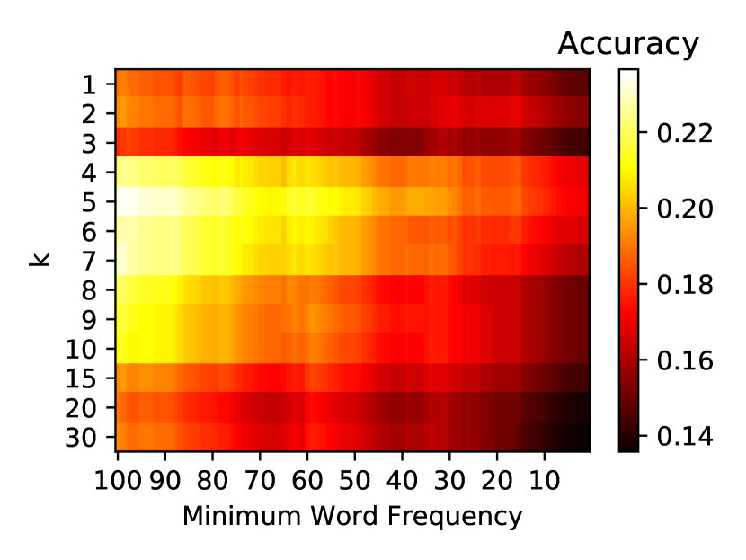
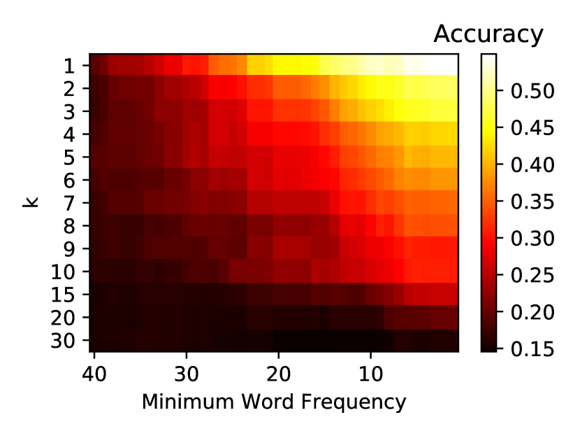
Figure 3(a) shows a clear pattern that as the minimum word frequency decreases, the -NN accuracy decreases no matter how changes. The pattern indicates that the low-frequency words are associated with the embedding vectors with low quality. Table 1 also shows that the self-embedding without low-frequency words (self(hf)) yields better performance. From Figure 3(b), we observed that the accuracy of -NN improve once the LSI is introduced, i.e., the embedding with LSI outperforms the vanilla embedding purely based on the training corpus by a large margin. The -NN accuracy also demonstrated improvement when we applied LSI to impute the subset of company names in the word2vec, Glove, and fastTest pre-trained embeddings. Such an improvement is evident in the low-frequency words.
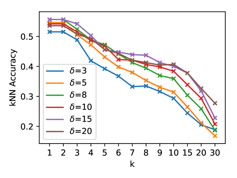
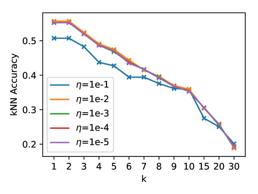
To verify whether LSI is robust to its hyper-parameter and stopping criterion , we did multiple investigations. When we set and let vary, we observed that LSI is relatively robust to a varying under the constraint that is not too large in which case the manifold assumption is significantly violated, or too small, which causes one or two neighbors to dominate. When we set the minimum degree of the graph and let vary, we also had the same observation that the LSI is robust to the stopping criterion .
5.2. Language Modeling on News Headlines
The straightforward way to measure the efficacy of different word embeddings is to feed them into a language model and inspect the perplexity. Language models are fundamental for many language tasks, including speech recognition, machine translation, parsing, and handwriting recognition. The goal of language modeling is to find the next most likely word following a word sequence, i.e., to maximize the conditional probability . Embedding words into a continuous Euclidean space (Bengio et al., 2003) is essential for the performance of language models.
We retrieved an experiment dataset from the Wharton Research Data Services (WRDS) and split the dataset into three folds: the training fold, which contains about 37.5k financial news headlines, and the validation and testing folds, each of which contains about 8k headlines. The corpus includes several thousand company names that are publicly listed on NYSE and NASDAQ. The dataset is small and it is difficult to attain reliable word embedding from the corpus directly. We adopted the three embeddings pre-trained on large corpora that also appeared in the previous experiment, used them as the initial embeddings to be enriched with domain knowledge, and recovered the embedding vectors for those missing company names via LSI.
In the pre-processing, we replaced the tokens with a frequency smaller than 3 with and used to denote End of Sentence. Those tokens that appear in the validation and testing folds and not in the training fold are also replaced with . The historical daily stock price data covers thousands of companies listed on NYSE and NASDAQ. We took the time series for 400 trading days ending on November 1, 2018, and removed those companies with more than 20% missing values. We used the daily return of these companies and filled the missing values with the mean of each day’s company return. The final data for the domain matrix contain 4092 companies, of which more than 3000 of these company names are not in the pre-trained embeddings.
We also trained an embedding matrix from scratch using the TensorFlow word2vec example code on the training set for language modeling. The learning rate is set to 0.1, the number of steps to two million, the minimum word frequency to 10, and the in the Gaussian initialization to 0.1. We name the obtained embedding “self-embedding” and use it as a baseline. The vocabulary for all embedding matrices is the same. For those missing vectors that can not be recovered by LSI, we randomly initialize them according to a Gaussian distribution with (the standard deviations of the word2vec, Glove, and fastText pre-trained embeddings along one dimension are 0.16, 0.38 and 0.25 respectively), and these randomly initialized word vectors will be updated by the neural net during training.
Our language model follows the TensorFlow benchmark for building a LSTM model on the Penn Bank Tree (PTB) dataset (small model settings) with some minor changes to the hyperparameters. We allow the model to use the pre-trained embedding and let it update the embedding vectors during training. We set the initial learning rate to 0.5 and let it decrease with a decay rate of 0.5 after two epochs. We found that the validation perplexity stopped declining and instead climbed up gradually at the end of epoch five, and thereby, we did an early stopping on the training. The language model with each embedding is trained ten times, and the result in Table 2 is the average decrease in perplexity.
| Embedding | Test PP | %decrease |
|---|---|---|
| self | 13.093 | |
| self+Google | 12.742 | 2.75 |
| self+fastText | 12.477 | 4.94 |
| self+Glove | 12.646 | 3.54 |
| 12.431 | 5.33 | |
| fastText | 12.215 | 7.19 |
| Glove | 12.218 | 7.16 |
| self+aff | 11.883 | 10.18 |
| Google+aff | 11.646 | 12.42 |
| fastText+aff | 11.638 | 12.51 |
| Glove+aff | 11.510 | 13.76 |
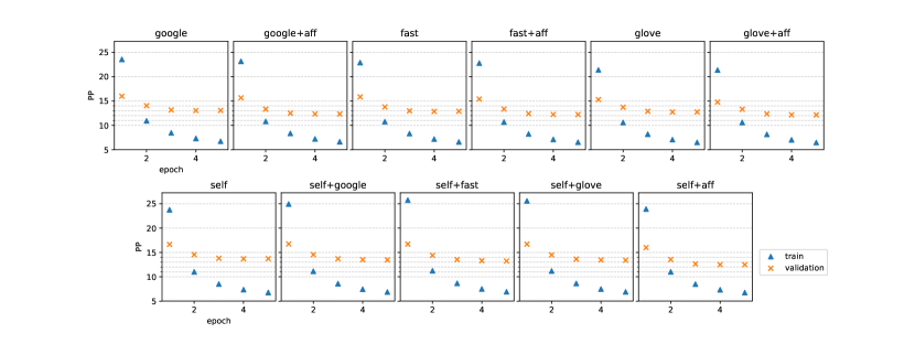
The experiment results show that the LSTM with self-embedding has the largest testing perplexity. In Table 2, we observed that the self-embedding plus general-purpose pre-trained embeddings via LSI leads to a 2-5% perplexity decrease. The observation demonstrates that when the corpus is small, it is difficult to obtain a reliable word embedding. In contrast, the pre-trained embedding on a vast corpus, such as Google-news with 100 billion words, is a better choice. However, the pre-trained embedding model on a large corpus is for the general purpose and will skip many keywords that are crucial to domain-specific language tasks. To obtain a more reliable domain-aware word embedding, we need to identify a domain-specific matrix and inject it into the general-purpose embedding. The Google-news (w2v), Glove and fastText pre-trained embeddings plus the domain matrix via LSI obtained an about 5% decrease in perplexity compared with those without LSI and a more than 12% decrease compared with the self-trained embedding.
6. Discussion and Conclusions
In this paper, we present a novel approach, Latent Semantic Imputation, for enhancing domain word embedding. It is capable of transferring prior knowledge from a domain matrix to the semantic space. LSI provides a novel approach to unifying the entity representations defined in different Euclidean spaces and has three major steps: (1) construct a Minimum-Spanning-Tree -Nearest-Neighbor graph from a domain matrix, (2) solve for the optimal weights using Non-Negative Least Squares, and (3) recover the missing embedding vectors in the semantic space using the power iteration method. LSI has only two hyper-parameters, the minimal degree of the graph and the stopping criterion in the power iteration step, and is robust to different values of the hyper-parameters. We also rigorously analyzed the deterministic convergence of LSI. Latent Semantic Imputation can be used for solving the problem of unreliable word embedding when the size of a training corpus is limited or when the critical domain words are missing from the vocabulary. Our experiments demonstrated how the frequency of a word negatively impacts the quality of word embedding and how LSI mitigates the impact. Specifically, the downstream language modeling with imputed embedding yields better performance than does the benchmark model pre-trained from large corpora.
7. Acknowledgements
Heartfelt thanks to Yiannis Koutis of NJIT and Xiangmin Jiao of Stony Brook University for their helpful discussions and to the anonymous reviewers for their comments.
References
- (1)
- Ahlswede et al. (2000) Rudolf Ahlswede, Ning Cai, S-YR Li, and Raymond W Yeung. 2000. Network information flow. IEEE Transactions on information theory 46, 4 (2000), 1204–1216.
- Belkin and Niyogi (2003) Mikhail Belkin and Partha Niyogi. 2003. Laplacian eigenmaps for dimensionality reduction and data representation. Neural computation 15, 6 (2003), 1373–1396.
- Bengio et al. (2006) Yoshua Bengio, Olivier Delalleau, and Nicolas Le Roux. 2006. 11 Label Propagation and Quadratic Criterion. (2006).
- Bengio et al. (2003) Yoshua Bengio, Réjean Ducharme, Pascal Vincent, and Christian Jauvin. 2003. A neural probabilistic language model. Journal of machine learning research 3, Feb (2003), 1137–1155.
- Bojanowski et al. (2016) Piotr Bojanowski, Edouard Grave, Armand Joulin, and Tomas Mikolov. 2016. Enriching word vectors with subword information. arXiv preprint arXiv:1607.04606 (2016).
- Bullinaria and Levy (2007) John A Bullinaria and Joseph P Levy. 2007. Extracting semantic representations from word co-occurrence statistics: A computational study. Behavior research methods 39, 3 (2007), 510–526.
- Deerwester et al. (1990) Scott Deerwester, Susan T Dumais, George W Furnas, Thomas K Landauer, and Richard Harshman. 1990. Indexing by latent semantic analysis. Journal of the American society for information science 41, 6 (1990), 391–407.
- Diamantaras and Kung (1996) Konstantinos I Diamantaras and Sun Yuan Kung. 1996. Principal component neural networks: theory and applications. Vol. 5. Wiley New York.
- Ganguly et al. (2015) Debasis Ganguly, Dwaipayan Roy, Mandar Mitra, and Gareth JF Jones. 2015. Word embedding based generalized language model for information retrieval. In Proceedings of the 38th international ACM SIGIR conference on research and development in information retrieval. ACM, 795–798.
- Harris (1954) Zellig S Harris. 1954. Distributional structure. Word 10, 2-3 (1954), 146–162.
- Hashimoto et al. (2016) Tatsunori B Hashimoto, David Alvarez-Melis, and Tommi S Jaakkola. 2016. Word embeddings as metric recovery in semantic spaces. Transactions of the Association for Computational Linguistics 4 (2016), 273–286.
- Hochreiter and Schmidhuber (1997) Sepp Hochreiter and Jürgen Schmidhuber. 1997. Long short-term memory. Neural computation 9, 8 (1997), 1735–1780.
- Huang et al. (2014) Hao Huang, Shinjae Yoo, Dantong Yu, and Hong Qin. 2014. Diverse power iteration embeddings and its applications. In Data Mining (ICDM), 2014 IEEE International Conference on. IEEE, 200–209.
- Jones et al. (2014) Eric Jones, Travis Oliphant, and Pearu Peterson. 2014. SciPy: open source scientific tools for Python. (2014).
- Kim (2014) Yoon Kim. 2014. Convolutional neural networks for sentence classification. arXiv preprint arXiv:1408.5882 (2014).
- Kruskal (1956) Joseph B Kruskal. 1956. On the shortest spanning subtree of a graph and the traveling salesman problem. Proceedings of the American Mathematical society 7, 1 (1956), 48–50.
- Lai et al. (2015) Siwei Lai, Liheng Xu, Kang Liu, and Jun Zhao. 2015. Recurrent Convolutional Neural Networks for Text Classification.. In AAAI, Vol. 333. 2267–2273.
- Lawson and Hanson (1995) Charles L Lawson and Richard J Hanson. 1995. Solving least squares problems. Vol. 15. Siam.
- Levy and Goldberg (2014) Omer Levy and Yoav Goldberg. 2014. Neural word embedding as implicit matrix factorization. In Advances in neural information processing systems. 2177–2185.
- Li et al. (2015) Yitan Li, Linli Xu, Fei Tian, Liang Jiang, Xiaowei Zhong, and Enhong Chen. 2015. Word Embedding Revisited: A New Representation Learning and Explicit Matrix Factorization Perspective.. In IJCAI. 3650–3656.
- Lin and Cohen (2010) Frank Lin and William W Cohen. 2010. Power Iteration Clustering.. In ICML, Vol. 10. Citeseer, 655–662.
- Liu et al. (2010) Wei Liu, Junfeng He, and Shih-Fu Chang. 2010. Large graph construction for scalable semi-supervised learning. In Proceedings of the 27th international conference on machine learning (ICML-10). 679–686.
- Lund and Burgess (1996) Kevin Lund and Curt Burgess. 1996. Producing high-dimensional semantic spaces from lexical co-occurrence. Behavior research methods, instruments, & computers 28, 2 (1996), 203–208.
- Maaten and Hinton (2008) Laurens van der Maaten and Geoffrey Hinton. 2008. Visualizing data using t-SNE. Journal of machine learning research 9, Nov (2008), 2579–2605.
- Mikolov et al. (2013a) Tomas Mikolov, Kai Chen, Greg Corrado, and Jeffrey Dean. 2013a. Efficient estimation of word representations in vector space. arXiv preprint arXiv:1301.3781 (2013).
- Mikolov et al. (2013b) Tomas Mikolov, Ilya Sutskever, Kai Chen, Greg S Corrado, and Jeff Dean. 2013b. Distributed representations of words and phrases and their compositionality. In Advances in neural information processing systems. 3111–3119.
- Mikolov et al. (2013c) Tomas Mikolov, Wen-tau Yih, and Geoffrey Zweig. 2013c. Linguistic regularities in continuous space word representations. In Proceedings of the 2013 Conference of the North American Chapter of the Association for Computational Linguistics: Human Language Technologies. 746–751.
- Mnih and Hinton (2009) Andriy Mnih and Geoffrey E Hinton. 2009. A scalable hierarchical distributed language model. In Advances in neural information processing systems. 1081–1088.
- Pennington et al. (2014) Jeffrey Pennington, Richard Socher, and Christopher Manning. 2014. Glove: Global vectors for word representation. In Proceedings of the 2014 conference on empirical methods in natural language processing (EMNLP). 1532–1543.
- Roweis and Saul (2000) Sam T Roweis and Lawrence K Saul. 2000. Nonlinear dimensionality reduction by locally linear embedding. science 290, 5500 (2000), 2323–2326.
- Saul and Roweis (2003) Lawrence K Saul and Sam T Roweis. 2003. Think globally, fit locally: unsupervised learning of low dimensional manifolds. Journal of machine learning research 4, Jun (2003), 119–155.
- Schnabel et al. (2015) Tobias Schnabel, Igor Labutov, David Mimno, and Thorsten Joachims. 2015. Evaluation methods for unsupervised word embeddings. In Proceedings of the 2015 Conference on Empirical Methods in Natural Language Processing. 298–307.
- Seneta (2006) Eugene Seneta. 2006. Non-negative matrices and Markov chains. Springer Science & Business Media.
- Sundermeyer et al. (2012) Martin Sundermeyer, Ralf Schlüter, and Hermann Ney. 2012. LSTM neural networks for language modeling. In Thirteenth annual conference of the international speech communication association.
- Turney and Pantel (2010) Peter D Turney and Patrick Pantel. 2010. From frequency to meaning: Vector space models of semantics. Journal of artificial intelligence research 37 (2010), 141–188.
- Von Luxburg (2007) Ulrike Von Luxburg. 2007. A tutorial on spectral clustering. Statistics and computing 17, 4 (2007), 395–416.
- Zhu and Ghahramani (2002) Xiaojin Zhu and Zoubin Ghahramani. 2002. Learning from labeled and unlabeled data with label propagation. Technical Report. Citeseer.