ALEX: An Updatable Adaptive Learned Index

Abstract.

Recent work on “learned indexes” has changed the way we look at the decades-old field of DBMS indexing. The key idea is that indexes can be thought of as “models” that predict the position of a key in a dataset. Indexes can, thus, be learned. The original work by Kraska et al. shows that a learned index beats a B+Tree by a factor of up to three in search time and by an order of magnitude in memory footprint. However, it is limited to static, read-only workloads.

In this paper, we present a new learned index called ALEX which addresses practical issues that arise when implementing learned indexes for workloads that contain a mix of point lookups, short range queries, inserts, updates, and deletes. ALEX effectively combines the core insights from learned indexes with proven storage and indexing techniques to achieve high performance and low memory footprint. On read-only workloads, ALEX beats the learned index from Kraska et al. by up to 2.2$\times$ on performance with up to 15$\times$ smaller index size. Across the spectrum of read-write workloads, ALEX beats B+Trees by up to 4.1$\times$ while never performing worse, with up to 2000$\times$ smaller index size. We believe ALEX presents a key step towards making learned indexes practical for a broader class of database workloads with dynamic updates.

1. Introduction

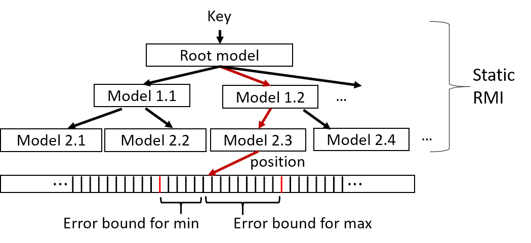
Recent work by Kraska et al. (Kraska et al., 2018), which we will refer to as the Learned Index, proposes to replace a standard database index with a hierarchy of machine learning (ML) models. Given a key, an intermediate node in the hierarchy is a model to predict the child model to use, and a leaf node in this hierarchy is a model to predict the location of the key in a densely packed array (Fig. 1). The models for this Learned Index are trained from the data. Their key insight is that using (even simple) models that adapt to the data distribution to make a “good enough” guess of a key’s actual location significantly improves performance. However, their solution can only handle lookups on read-only data, with no support for update operations. This critical drawback makes the Learned Index unusable for dynamic, read-write workloads, common in practice.

In this work, we start by asking ourselves the following research question: Can we design a new high performance index for dynamic workloads that effectively combines the core insights from the Learned Index with proven storage & indexing techniques to deliver great performance in both time and space? Our answer is a new in-memory index structure called ALEX, a fully dynamic data structure that simultaneously provides efficient support for point lookups, short range queries, inserts, updates, deletes, and bulk loading. This mix of operations is commonplace in online transaction processing (OLTP) workloads (Cooper et al., 2010; TPC, [n.d.]; Cao et al., 2020) and is also supported by B+Trees (Ramakrishnan and Gehrke, 2002).

Implementing writes with high performance requires a careful design of the underlying data structure that stores records. (Kraska et al., 2018) uses a sorted, densely packed array which works well for static datasets but can result in high costs for shifting records if new records are inserted. Furthermore, the prediction accuracy of the models can deteriorate as the data distribution changes over time, requiring repeated retraining. To address these challenges, we make the following technical contributions in this paper:

• Storage layout optimized for models: Similar to a B+Tree, ALEX builds a tree, but allows different nodes to grow and shrink at different rates. To store records in a data node, ALEX uses an array with gaps, a Gapped Array, which (1) amortizes the cost of shifting the keys for each insertion because gaps can absorb inserts, and (2) allows more accurate placement of data using model-based inserts to ensure that records are located closely to the predicted position when possible. For efficient search, gaps are actually filled with adjacent keys.

• Search strategy optimized for models: ALEX exploits model-based inserts combined with exponential search starting from the predicted position. This always beats binary search when models are accurate.

• Keeping models accurate with dynamic data distributions and workloads: ALEX provides robust performance even when the data distribution is skewed or dynamically changes after index initialization. ALEX achieves this by exploiting adaptive expansion, and node splitting mechanisms, paired with selective model retraining, which is triggered by intelligent policies based on simple cost models. Our cost models take the actual workload into account and thus can effectively respond to dynamic changes in the workload. ALEX achieves all the above benefits without needing to hand-tune parameters for each dataset or workload.

• Detailed evaluation: We present the results of an extensive experimental analysis with real-life datasets and varying read-write workloads and compare against state of the art indexes that support range queries.

On read-only workloads, ALEX beats the Learned Index by up to 2.2$\times$ on performance with up to 15$\times$ smaller index size. Across the spectrum of read-write workloads, ALEX beats B+Tree by up to 4.1$\times$ while never performing worse, with up to 2000$\times$ smaller index size. ALEX also beats an ML-enhanced B+Tree and the memory-optimized Adaptive Radix Tree, scales to large data sizes, and is robust to data distribution shift.

In the remainder of this paper, we give background (Section 2), present the architecture of ALEX (Section 3), describe the operations on ALEX (Section 4), present an analysis of ALEX performance (Section 5), present experimental results (Section 6), review related work (Section 7), and conclude (Section 8).

2. Background

2.1. Traditional B+Tree Indexes

B+Tree is a classic range index structure. It is a height-balanced tree which stores either the data (primary index) or pointers to the data (secondary index) at the leaf level, in a sorted order to facilitate range queries.

A B+Tree lookup operation can be broken down into two steps: (1) traverse to leaf, and (2) search within the leaf. Starting at the root, traverse to leaf performs comparisons with the keys stored in each node, and branches via stored pointers to the next level. When the tree is deep, the number of comparisons and branches can be large, leading to many cache misses. Once traverse to leaf identifies the correct leaf page, typically a binary search is performed to find the position of the key within the node, which might incur additional cache misses.

The B+Tree is a dynamic data structure that supports inserts, updates, and deletes; is robust to data sizes and distributions; and is applicable in many different scenarios, including in-memory and on-disk. However, the generality of B+Tree comes at a cost. In some cases knowledge of the data helps improve performance. As an extreme example, if the keys are consecutive integers, we can store the data in an array and perform lookup in ${\rm O}(1)$ time. A B+Tree does not exploit such knowledge. Here, “learning” from the input data has an edge.

Figure 1. Learned Index by Kraska et al.

2.2. The Case for Learned Indexes

Kraska et al. (Kraska et al., 2018) observed that B+Tree indexes can be thought of as models. Given a key, they predict the location of the key within a sorted array (logically) at the leaf level. If indexes are models, they can be learned using traditional ML techniques by learning the cumulative distribution function (CDF) of the input data. The resulting Learned Index is optimized for the specific data distribution.

Another insight from Kraska et al. is that a single ML model learned over the entire data is not accurate enough because of the complexity of the CDF. To overcome this, they introduce the recursive model index (RMI) (Kraska et al., 2018). RMI is a hierarchy of models, with a static depth of two or three, where a higher-level model picks the model at the next level, and so on, with the leaf-level model making the final prediction for the position of the key in the data structure (Fig. 1). Logically, the RMI replaces the internal B+Tree nodes with models. The effect is that comparisons and branches in internal B+Tree nodes during traverse to leaf are replaced by model inferences in a Learned Index.

In (Kraska et al., 2018), the keys are stored in an in-memory sorted array. Given a key, the leaf-level model predicts the position (array index) of the key. Since the model is not perfect, it could make a wrong prediction. The insight is that if the leaf model is accurate, a local search surrounding the predicted location is faster than a binary search on the entire array. To support local search,  (Kraska et al., 2018) keeps min and max error bounds for each model in RMI and performs binary search within these bounds.

Last, each model in RMI can be a different type of model. Both linear regression and neural network based models are considered in (Kraska et al., 2018). There is a trade-off between model accuracy and model complexity. The root of the RMI is tuned to be either a neural network or a linear regression, depending on which provides better performance, while the simplicity and the speed of computation for linear regression model is beneficial at the non-root levels. A linear regression model can be represented as $y=\lfloor a*x+b\rfloor$, where $x$ is the key and $y$ is the predicted position. A linear regression model needs to store just two parameters $a$ and $b$, so storage overhead is low. The inference with a single linear regression model requires only one multiplication, one addition and one rounding, which are fast to execute on modern processors.

Unlike B+Tree, which could have many internal levels, RMI uses two or three levels. Also, the storage space required for models (two or four 8-byte double values per model) is much smaller than the storage space for internal nodes in B+Tree (which store keys and pointers). A Learned Index can be an order of magnitude smaller in main memory storage (vs. internal B+Tree nodes), while outperforming a B+Tree in lookup performance by a factor of up to three (Kraska et al., 2018).

The main drawback of the Learned Index is that it does not support any modifications, including inserts, updates, or deletes. Let us demonstrate a naïve insertion strategy for such an index. Given a key $k$ to insert, we first use the model to find the insertion position for $k$. Then we create a new array whose length is one plus the length of the old array. Next, we copy the data from the old array to the new array, where the elements on the right of the insertion position are shifted to the right by one position. We insert $k$ at the insertion position of the new array. Finally, we update the models to reflect the change in the data distribution. Such a strategy has a linear time complexity with respect to the data size, which is unacceptable in practice. Kraska et al. suggest building delta-indexes to handle inserts (Kraska et al., 2018), which is complementary to our strategy. In this paper, we describe an alternative data structure to make modifications in a learned index more efficient.

3. ALEX Overview

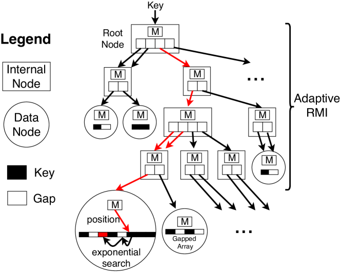
The ALEX design (Fig. 2) takes advantage of two key insights. First, we propose a careful space-time trade-off that not only leads to an updatable data structure, but is also faster for lookups. To explore this trade-off, ALEX supports a Gapped Array (GA) layout for the leaf nodes, which we present in Section 3.2. Second, the Learned Index supports static RMI (SRMI) only, where the number of levels and the number of models in each level is fixed at initialization. SRMI performs poorly on inserts if the data distribution is difficult to model. ALEX can be updated dynamically and efficiently at runtime and uses linear cost models that predict the latency of lookup and insert operations based on simple statistics measured from an RMI. ALEX uses these cost models to initialize the RMI structure and to dynamically adapt the RMI structure based on the workload.

ALEX aims to achieve the following goals w.r.t. the B+Tree and Learned Index. (1) Insert time should be competitive with B+Tree, (2) lookup time should be faster than B+Tree and Learned Index, (3) index storage space should be smaller than B+Tree and Learned Index (4) data storage space (leaf level) should be comparable to dynamic B+Tree. In general, data storage space will overshadow index storage space, but the space benefit from smaller index storage space is still important because it allows more indexes to fit into the same memory budget. The rest of this section describes how our ALEX design achieves these goals.

Figure 2. ALEX Design

3.1. Design Overview

ALEX is an in-memory, updatable learned index. ALEX has a number of differences from the Learned Index (Kraska et al., 2018).

The first difference lies in the data structure used to store the data at the leaf level. Like B+Tree, ALEX uses a node per leaf. This allows the individual nodes to expand and split more flexibly and also limits the number of shifts required during an insert. In a typical B+Tree, every leaf node stores an array of keys and payloads and has “free space” at the end of the array to absorb inserts. ALEX uses a similar design but more carefully chooses how to use the free space. The insight is that by introducing gaps that are strategically placed between elements of the array, we can achieve faster insert and lookup times. As shown in Fig. 2, ALEX uses a Gapped Array (GA) layout for each data node, which we describe in Section 3.2.

The second difference is that ALEX uses exponential search to find keys at the leaf level to correct mispredictions of the RMI, as shown in Fig. 2. In contrast, (Kraska et al., 2018) uses binary search within the error bounds provided by the models. We experimentally verified that exponential search without bounds is faster than binary search with bounds (Section 6.3.1). This is because if the models are good, their prediction is close enough to the correct position. Exponential search also removes the need to store error bounds in the models of the RMI.

The third difference is that ALEX inserts keys into data nodes at the position where the models predict that the key should be. We call this model-based insertion. In contrast, the Learned Index produces an RMI on an array of records without changing the position of records in the array. Model-based insertion has better search performance because it reduces model misprediction errors.

The fourth difference is that ALEX dynamically adjusts the shape and height of the RMI depending on the workload. We describe the design of initializing and dynamically growing the RMI structure in Section 4.

The final difference is that ALEX has no parameters that need to be re-tuned for each dataset or workload, unlike the Learned Index, in which the number of models must be tuned. ALEX automatically bulk loads and adjusts the structure of RMI to achieve high performance by using a cost model.

3.2. Node Layout

3.2.1. Data Nodes

Like a B+Tree, the leaf nodes of ALEX store the data records and thus are referred to as data nodes, shown as circles in Fig. 2. A data node stores a linear regression model (two double values for slope and intercept), which maps a key to a position, and two Gapped Arrays (described below), one for keys and one for payloads. We show only the keys array in Fig. 2. By default, both keys and payloads are fixed-size. (Note that payloads could be records or pointers to variable-sized records, stored in separately allocated spaces in memory). We also impose a max node size for practical reasons (see details in Section 4).

ALEX uses a Gapped Array layout which uses model-based inserts to distribute extra space between the elements of the array, thereby achieving faster inserts and lookups. In contrast, B+Tree places all the gaps at the end of the array. Gapped Arrays fill the gaps with the closest key to the right of the gap, which helps maintain exponential search performance. In order to efficiently skip gaps when scanning, each data node maintains a bitmap which tracks whether each location in the node is occupied by a key or is a gap. The bitmap is fast to query and has low space overhead compared to the Gapped Array. We compare Gapped Array to an existing gapped data structure called Packed Memory Array (Bender and Hu, 2007) in Section E.

3.2.2. Internal Nodes

We refer to all the nodes which are part of the RMI structure as internal nodes, shown as rectangles in Fig. 2. Internal nodes store a linear regression model and an array containing pointers to children nodes. Like a B+Tree, internal nodes direct traversals down the tree, but unlike B+Tree, internal nodes in ALEX use models to “compute” the location, in the pointers array, of the next child pointer to follow. Similar to data nodes, we impose a max node size.

(a)

(b)

Figure 3. Internal nodes allow different resolutions in different parts of the key space $[0,1)$.

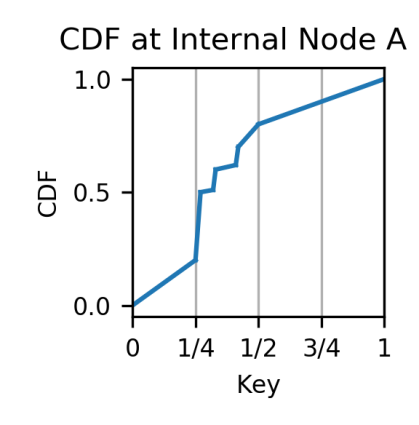
The internal nodes of ALEX serve a conceptually different purpose than those of the Learned Index. Learned Index’s internal nodes have models that are fit to the data; an internal node with a perfect model partitions keys equally to its children, and an RMI with perfect internal nodes results in an equal number of keys in each data node. However, the goal of the RMI structure is not to produce equally sized data nodes, but rather data nodes whose key distributions are roughly linear, so that a linear model can be accurately fit to its keys.

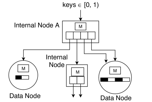
Therefore, the role of the internal nodes in ALEX is to provide a flexible way to partition the key space. Suppose internal node A in Fig. 3 covers the key space $[0,1)$ and has four child pointers. A Learned Index would assign a node to each of these pointers, either all internal nodes or all data nodes. However, ALEX more flexibly partitions the space. Internal node A assigns the key spaces $[0,1/4)$ and $[1/2,1)$ to data nodes (because the CDF in those spaces are linear), and assigns $[1/4,1/2)$ to another internal node (because the CDF is non-linear and the RMI requires more resolution into this key space). As shown in the figure, multiple pointers can point to the same child node; this is useful for handling inserts (Section 4.3.3). We restrict the number of pointers in every internal node to always be a power of 2. This allows nodes to split without retraining its subtree (Section 4.3.3).

4. ALEX Algorithms

In this section, we describe the algorithms for lookups, inserts (including how to dynamically grow the RMI and the data nodes), deletes, out of bounds inserts, and bulk load.

4.1. Lookups and Range Queries

To look up a key, starting at the root node of the RMI, we iteratively use the model to “compute” a location in the pointers array, and we follow the pointer to a child node at the next level, until we reach a data node. By construction, the internal node models have perfect accuracy, so there is no search involved in the internal nodes. We use the model in the data node to predict the position of the search key in the keys array, doing exponential search if needed to find the actual position of the key. If a key is found, we read the corresponding value at the same position from the payloads array and return the record. Else, we return a null record. We visually show (using red arrows) a lookup in Fig. 2. A range query first performs a lookup to find the position and data node of the first key whose value is not less than the range’s start value, then scans forward until reaching the range’s end value, using the node’s bitmap to skip over gaps and if necessary using pointers stored in the node to jump to the next data node.

4.2. Insert in non-full Data Node

For the insert algorithm, the logic to reach the correct data node (i.e., TraverseToLeaf) is the same as in the lookup algorithm described above. In a non-full data node, to find the insertion position for a new element, we use the model in the data node to predict the insertion position. If the predicted position is not correct (if inserting there would not maintain sorted order), we do exponential search to find the correct insertion position. If the insertion position is a gap, then we insert the element into the gap and are done. Else, we make a gap at the insertion position by shifting the elements by one position in the direction of the closest gap. We then insert the element into the newly created gap. The Gapped Array achieves $O(\log{n})$ insertion time with high probability (Bender et al., 2006).

Figure 4. Node Expansion

(a)

(b)

(c)

Figure 5. Node Splits

4.3. Insert in full Data Node

When a data node becomes full, ALEX uses two mechanisms to create more space: expansions and splits. ALEX relies on simple cost models to pick between different mechanisms. Below, we first define the notion of “fullness,” then describe the expansion and split mechanisms, and the cost models. We then present the insertion algorithm that combines the mechanisms with the cost models. Algorithm 1 summarizes the procedure for inserting into a data node.

4.3.1. Criteria for Node Fullness

ALEX does not wait for a data node to become 100% full, because insert performance on a Gapped Array will deteriorate as the number of gaps decreases. We introduce lower and upper density limits on the Gapped Array: $d_{l},d_{u}\in(0,1]$, with the constraint that $d_{l}<d_{u}$. Density is defined as the fraction of positions that are filled by elements. A node is full if the next insert results in exceeding $d_{u}$. By default we set $d_{l}=0.6$ and $d_{u}=0.8$ to achieve average data storage utilization of $0.7$, similar to B+Tree (Graefe, 2011), which in our experience always produces good results and did not need to be tuned. In contrast, B+Tree nodes typically have $d_{l}=0.5$ and $d_{u}=1$. Section 5 presents a theoretical analysis of how the density of the Gapped Array provides a way to trade off between the space and the lookup performance for ALEX.

4.3.2. Node Expansion Mechanism

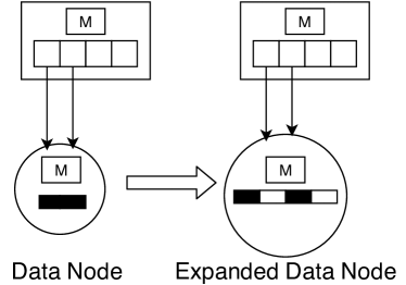
To expand a data node that contains $n$ keys, we allocate a new larger Gapped Array with $n/d_{l}$ slots. We then either scale or retrain the linear regression model, and then do model-based inserts of all the elements in this new larger node using the scaled or retrained model. After creation, the new data node is at the lower density limit $d_{l}$. Fig. 4 shows an example data node expansion where the Gapped Array inside the data node is expanded from two slots on the left to four slots on the right.

4.3.3. Node Split Mechanism

To split a data node in two, we allocate the keys to two new data nodes, such that each new node is responsible for half of the key space of the original node. ALEX supports two ways to split a node:

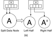
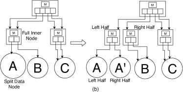
(1) Splitting sideways is conceptually similar to how a B+Tree uses splits. There are two cases: (a) If the parent internal node of the split data node is not yet at the max node size, we replace the parent node’s pointers to the split data node with pointers to the two new data nodes. The parent internal node’s pointers array might have redundant pointers to the split data node (Fig. 3). If so, we give half of the redundant pointers to each of the two new nodes. Else, we create a second pointer to the split data node by doubling the size of the parent node’s pointers array and making a redundant copy for every pointer, and then give one of the redundant pointers to each of the two new nodes. Fig. 5a shows an example of a sideways split that does not require an expansion of the parent internal node. (b) If the parent internal node has reached max node size, then we can choose to split the parent internal node, as we show in Fig. 5b. Note that by restricting all the internal node sizes to be powers of 2, we can always split a node in a “boundary preserving” way, and thus require no retraining of any models below the split internal node. Note that the split can propagate all the way to the root node, just like in a B+Tree.

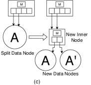
(2) Splitting down converts a data node into an internal node with two child data nodes, as we show in Fig. 5c. The models in the two child data nodes are trained on their respective keys. B+Tree does not have an analogous splitting down mechanism.

4.3.4. Cost Models

To make decisions about which mechanism to apply (expansion or various types of splits), ALEX relies on simple linear cost models that predict average lookup time and insert time based on two simple statistics tracked at each data node: (a) average number of exponential search iterations, and (b) average number of shifts for inserts. Lookup performance is directly correlated with (a) while insert performance is directly correlated with (a) and (b) (since an insert first needs to do a lookup to find the correct insertion position). These intra-node cost models predict the time to perform operations within a data node.

These two statistics are not known when creating a data node. To find the expected cost of a new data node, we compute the expected value of these statistics under the assumption that lookups are done uniformly on the existing keys, and inserts are done according to the existing key distribution. Specifically, (a) is computed as the average base-2 logarithm of model prediction error for all keys; (b) is computed as the average distance to the closest gap in the Gapped Array for all existing keys. These expected values can be computed without creating the data node. If the data node is created using a subset of keys from an existing data node, we can use the empirical ratio of lookups vs. inserts to weight the relative importance of the two statistics for computing the expected cost.

In addition to the intra-node cost model, ALEX uses a TraverseToLeaf cost model to predict the time for traversing from the root node to a data node. The TraverseToLeaf cost model uses two statistics: (1) the depth of the data node being traversed to, and (2) the total size (in bytes) of all inner nodes and data node metadata (i.e., everything except for the keys and payloads). These statistics capture the cost of traversal: deeper data nodes require more pointer chases to find, and larger size will decrease CPU cache locality, which slows down the traversal to a data node. We provide more details about the cost models and show their low usage overhead in Section D.

4.3.5. Insertion Algorithm

As lookups and inserts are done on the data node, we count the number of exponential search iterations and shifts per insert. From these statistics, we compute the empirical cost of the data node using the intra-node cost model. Once the data node is full, we compare the expected cost (computed at node creation time) to the empirical cost. If they do not deviate significantly, then we conclude that the model is still accurate, and we perform node expansion (if the size after expansion is less than the max node size), scaling the model instead of retraining. The models in the internal nodes of the RMI are not retrained or rescaled. We define significant cost deviation as occurring when the empirical cost is more than 50% higher than the expected cost. In our experience, this cost deviation threshold of 50% always produces good results and did not need to be tuned.

Otherwise, if the empirical cost has deviated from the expected cost, we must either (i) expand the data node and retrain the model, (ii) split the data node sideways, or (iii) split the data node downwards. We select the action that results in lowest expected cost, according to our intra-node cost model. For simplicity, ALEX always splits a data node in two. The data node could conceptually split into any power of 2, but deciding the optimal fanout can be time-consuming, and we experimentally verified that a fanout of 2 is best according to the cost model in most cases.

4.3.6. Why would empirical cost deviate from expected cost?

This often happens when the distribution of keys that are inserted does not follow the distribution of existing keys, which results in the model becoming inaccurate. An inaccurate model may lead to long contiguous regions without any gaps. Inserting into these fully-packed regions requires shifting up to half of the elements within it to create a gap, which in the worst case takes $O(n)$ time. Performance may also degrade simply due to random noise as the node grows larger or due to changing access patterns for lookups.

Algorithm 1 Gapped Array Insertion

1:struct Node $\{$ keys[] (Gapped Array); num_keys; $d_{u},d_{l}$;     model: key$\rightarrow[0,$ keys.size); $\}$

2:procedure Insert($key$)

3:    if num_keys / keys.size ¿= $d_{u}$ then

4:         if expected cost $\approx$ empirical cost then

5:             Expand(retrain=False)

6:         else

7:             Action with lowest cost /* described in Sec. 4.3.5 */

8:         end if

9:    end if

10:    predicted_pos = model.predict(key)

11:    /* check for sorted order */

12:    insert_pos = CorrectInsertPosition(predicted_pos)

13:    if  keys[insert_pos] is occupied  then

14:         MakeGap(insert_pos) /* described in text */

15:    end if

16:    keys[insert_pos] = key

17:    num_keys++

18:end procedure

19:procedure Expand($retrain$)

20:    expanded_size = num_keys * 1/$d_{l}$

21:    /* allocate a new expanded array */

22:    expanded_keys = array(size=expanded_size)

23:    if retrain == True then

24:         model = /* train linear model on keys */

25:    else

26:         /* scale existing model to expanded array */

27:         model *= expanded_size / keys.size

28:    end if

29:    for key : keys do

30:         ModelBasedInsert(key)

31:    end for

32:    keys = expanded_keys

33:end procedure

34:procedure ModelBasedInsert($key$)

35:    insert_pos = model.predict(key)

36:    if keys[insert_pos] is occupied then

37:         insert_pos = first gap to right of predicted_pos

38:    end if

39:    keys[insert_pos] = key

40:end procedure

4.4. Delete, update, and other operations

To delete a key, we do a lookup to find the location of the key, and then remove it and its payload. Deletes do not shift any existing keys, so deletion is a strictly simpler operation than inserts and does not cause model accuracy to degrade. If a data node hits the lower density limit $d_{l}$ due to deletions, then we contract the data node (i.e., the opposite of expanding the data node) in order to avoid low space utilization. Additionally, we can use intra-node cost models to determine that two data nodes should merge together and potentially grow upwards, locally decreasing the RMI depth by 1. However, for simplicity we do not implement these merging operations.

Updates that modify the key are implemented by combining an insert and a delete. Updates that only modify the payload will look up the key and write the new value into the payload. Like B+Trees, we can merge two ALEX indexes or find the difference between two ALEX indexes by iterating over their sorted keys in tandem and bulk loading a new ALEX index.

4.5. Handling out of bounds inserts

A key that is lower or higher than the existing key space would be inserted into the the left-most or right-most data node, respectively. A series of out-of-bounds inserts, such as an append-only insert workload, would result in poor performance because that data node has no mechanism to split the out-of-bounds key space. Therefore, ALEX has two ways to smoothly handle out-of-bounds inserts. Assume that the out-of-bounds inserts are to the right (e.g., inserted keys are increasing); we apply analogous strategies when inserts are to the left.

Figure 6. Splitting the root

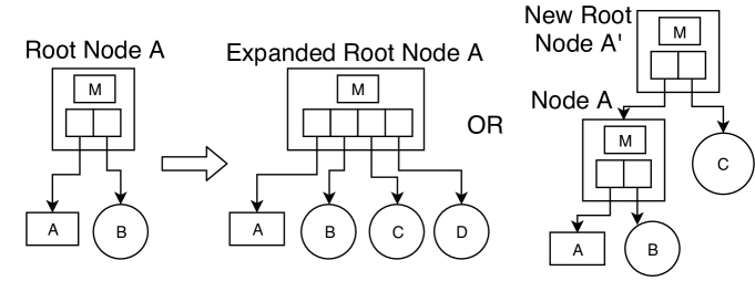
First, when an insert that is outside the existing key space is detected, ALEX will expand the root node, thereby expanding the key space, shown in Fig. 6. We expand the size of the child pointers array to the right. Existing pointers to existing children are not modified. A new data node is created for every new slot in the expanded pointers array. In case this expansion would result in the root node exceeding the max node size, ALEX will create a new root node. The first child pointer of the new root node will point to the old root node, and a new data node is created for every other pointer slot of the new root node. At the end of this process, the out-of-bounds key will fall into one of the newly created data nodes.

Second, the right-most data node of ALEX detects append-only insertion behavior by maintaining the value of the maximum key in the node and keeping a counter for how many times an insert exceeds that maximum value. If most inserts exceed the maximum value, that implies append-only behavior, so the data node expands to the right without doing model-based re-insertion; the expanded space is kept initially empty in anticipation of more append-like inserts.

4.6. Bulk Load

ALEX supports a bulk load operation, which is used in practice to index large amounts of data at initialization or for rebuilding an index. Our goal is to find an RMI structure with minimum cost, defined as the expected average time to do an operation (i.e., lookup or insert) on this RMI. Any ALEX operation is composed of TraverseToLeaf to the data node followed by an intra-node operation, so RMI cost is modeled by combining the TraverseToLeaf and intra-node cost models.

4.6.1. Bulk Load Algorithm

Using the cost models, we grow an RMI downwards greedily, starting from the root node. At each node, we independently make a decision about whether the node should be a data node or an internal node, and in the latter case, what the fanout should be. The fanout must be a power of 2, and child nodes will equally divide the key space of the current node. Note that we can make this decision locally for each node because we use linear cost models, so decisions will have a purely additive effect on the overall cost of the RMI. If we decide the node should be an internal node, we recurse on each of its child nodes. This continues until all the data is loaded in ALEX.

Figure 7. Fanout Tree

4.6.2. The Fanout Tree

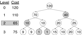
As we grow the RMI, the main challenge is to determine the best fanout at each node. We introduce the concept of a fanout tree (FT), which is a complete binary tree. An FT will help decide the fanout for a single RMI node; in our bulk loading algorithm, we construct an FT each time we want to decide the best fanout for an RMI node. A fanout of 1 means that the RMI node should be a data node.

Fig. 7 shows an example FT. Each FT node represents a possible child of the RMI node. If the key space of the RMI node is $[0,1)$, then the $i$-th FT node on a level with $n$ children represents a child RMI node with key space $[i/n,(i+1)/n)$. Each FT node is associated with the expected cost of constructing a data node over its key space, as predicted by the intra-node cost models. Our goal is to find a set of FT nodes that cover the entire key space of the RMI node with minimum overall cost. The overall cost of a covering set is the sum of the costs of its FT nodes, as well as the TraverseToLeaf cost due to model size (e.g., going a level deeper in the FT means the RMI node must have twice as many pointers). This covering set determines the optimal fanout of the RMI node (i.e., the number of child pointers) as well as the optimal way to allocate child pointers.

We use the following method to find a low-cost covering set: (1) Starting from the FT root, grow entire levels of the FT at a time, and compute the cost of using each level as the covering set. Continue doing so until the costs of each successive level start to increase. In Fig. 7, we find that level 2 has the lowest combined cost, and we do not keep growing after level 3. In concept, a deeper level might have lower cost, but computing the cost for each FT node is expensive. (2) Starting from the level of the FT with lowest combined cost, we start merging or splitting FT nodes locally. If the cost of two adjacent FT nodes is higher than the cost of its parent, then we merge (e.g., the nodes with cost 20 and 25 are merged to one with cost 40); this might happen when the two nodes have very few keys, or when their distributions are similar. In the other direction, if the cost of a FT node is higher than the cost of its two children, we split the FT node (e.g., the node with cost 10 is split into two nodes each with cost 1); this might happen when the two halves of the key space have different distributions. We continue with this process of merging and splitting adjacent nodes locally until it is no longer possible. We return the resulting covering set of FT nodes.

5. Analysis of ALEX

In this section, we provide bounds on the RMI depth and complexity analysis. Bounds on the performance of model-based search are found in Section F.

5.1. Bound on RMI depth

In this section we present a worst-case bound on maximum RMI depth and describe how to achieve it. Note that the goal of ALEX is to maximize performance, not to minimize tree depth; though the two are correlated, the latter is simply a proxy for the former (e.g., depth is one input to our cost models). Therefore, this analysis is useful for gaining intuition about RMI depth, but does not reflect worst-case guarantees in practice.

Let $m$ be the maximum node size, defined in number of slots (in the pointers array for internal nodes, in the Gapped Array for data nodes). We constrain node size to be a power of 2: $m=2^{k}$. Internal nodes can have up to $m$ child pointers, and data nodes must contain no more than $md_{u}$ keys. Let all keys to be indexed fall within the key space $s$. Let $p$ be the minimum number of partitions such that when the key space $s$ is divided into $p$ partitions of equal width, every partition contains no more than $md_{u}$ keys. Define the root node depth as 0.

Theorem 5.1.

We can construct an RMI that satisfies the max node size and upper density limit constraints whose depth is no larger than $\lceil\log_{m}{p}\rceil$—we call this the maximal depth. Furthermore, we can maintain maximal depth under inserts. (Note that $p$ might change under inserts.)

In other words, the depth of the RMI is bounded by the density of the densest subregion of $s$. In contrast, B+Trees bound depth as a function of the number of keys. Theorem 5.1 can also be applied to a subspace within $s$, which would correspond to some subtree within the RMI.

Proof.

Constructing an RMI with maximal depth is straightforward. The densest subregion, which spans a key space of size $|s|/p$, is allocated to a data node. The traversal path from the root to this densest region is composed of internal nodes, each with $m$ child pointers. It takes $\lceil\log_{m}{p}\rceil$ internal nodes to narrow the key space size from $|s|$ to $|s|/p$. To minimize depth in other subtrees of the RMI, we apply this construction mechanism recursively to the remaining parts of the space $s$.

Starting from an RMI that satisfies maximal depth, we maintain maximal depth using the mechanisms in Section 4.3 under the following policy: (1) Data nodes expand until they reach max node size. (2) When a data node must split due to max node size, it splits sideways to maintain current depth (potentially propagating the split up to some ancestor internal node). (3) When splitting sideways is no longer possible (all ancestor nodes are at max node size), split downwards. By following this policy, RMI only splits downward when $p$ grows by a factor of $m$, thereby maintaining maximal depth. ∎

5.2. Complexity analysis

Here we provide complexity of lookups and inserts, as well as the mechanisms from Section 4.3. Both lookups and inserts do TraverseToLeaf in $\lceil\log_{m}{p}\rceil$ time. Within the data node, exponential search for lookups is bounded in the worst case by $O(\log{m})$. In the best case, the data node model predicts the key’s position perfectly, and lookup takes $O(1)$ time. We show in the next sub-section that we can reduce exponential search time according to a space-time trade-off.

Inserts into a non-full node are composed of a lookup, potentially followed by shifts to introduce a gap for the new key. This is bounded in the worst case by $O(m)$, but since Gapped Array achieves $O(\log{m})$ shifts per insert with high probability (Bender et al., 2006), we expect $O(\log{m})$ complexity in most cases. In the best case, the predicted insertion position is correct and is a gap, and we place the key exactly where the model predicts for insert complexity of $O(1)$; furthermore, a later model-based lookup will result in a direct hit in $O(1)$.

There are three important mechanisms in Section 4.3, whose costs are defined by how many elements must be copied: (1) Expansion of a data node, whose cost is bounded by $O(m)$. (2) Splitting downwards into two nodes, whose cost is bounded by $O(m)$. (3) Splitting sideways into two nodes and propagating upwards in the path to some ancestor node, whose cost is bounded by $O(m\lceil\log_{m}{p}\rceil)$ because every internal node on this path must also split. As a result, the worst-case performance for insert into a full node is $O(m\lceil\log_{m}{p}\rceil)$.

6. Evaluation

We compare ALEX with the Learned Index, B+Tree, a model-enhanced B+Tree, and Adaptive Radix Tree (ART), using a variety of datasets and workloads. This evaluation demonstrates that:

• On read-only workloads, ALEX achieves up to 4.1$\times$, 2.2$\times$, 2.9$\times$, 3.0$\times$ higher throughput and 800$\times$, 15$\times$, 160$\times$, 8000$\times$ smaller index size than the B+Tree, Learned Index, Model B+Tree, and ART, respectively.

• On read-write workloads, ALEX achieves up to 4.0$\times$, 2.7$\times$, 2.7$\times$ higher throughput and 2000$\times$, 475$\times$, 36000$\times$ smaller index size than the B+Tree, Model B+Tree, and ART, respectively.

• ALEX has competitive bulk load times and maintains an advantage over other indexes when scaling to larger datasets and under distribution shift due to data skew.

• Gapped Array and the adaptive RMI structure allow ALEX to adapt to different datasets and workloads.

6.1. Experimental Setup

We implement ALEX in C++. We perform our evaluation via single-threaded experiments on an Ubuntu Linux machine with Intel Core i9-9900K 3.6GHz CPU and 64GB RAM. We compare ALEX against four baselines. (1) A standard B+Tree, as implemented in the STX B+Tree (Bingmann, [n.d.]). (2) Our best-effort reimplementation of the Learned Index (Kraska et al., 2018), using a two-level RMI with linear models at each node and binary search for lookups. (3) Model B+Tree, which maintains a linear model in every node of the B+Tree, stores each node as a Gapped Array, and uses model-based exponential search instead of binary search, implemented on top of (Bingmann, [n.d.]); this shows the benefit of using models while keeping the fundamental B+Tree structure. (4) Adaptive Radix Tree (ART) (Leis et al., 2013), a trie that adapts to the data which is optimized for main memory indexing, implemented in C (Dadgar, [n.d.]). Since ALEX supports all operations common in OLTP workloads, we do not compare to hash tables and dynamic hashing techniques, which cannot efficiently support range queries.

For each dataset and workload, we use grid search to tune the page size for B+Tree and Model B+Tree and the number of models for Learned Index to achieve the best throughput. In contrast, no tuning is necessary for ALEX, unless users place additional constraints. For example, users might want to bound the latency of a single operation. We set a max node size of 16MB to achieve tail latency (99.9th percentile) of around 2$\mu$s per operation, but max node size can be adjusted according to user’s desired limits (Fig. 16).

Index size of ALEX and Learned Index is the sum of the sizes of all models used in the index and metadata; index size for ALEX also includes internal node pointers. For ALEX, each linear model consists of two 64-bit doubles which represent the slope and intercept. Learned Index keeps two additional integers per model that represent the error bounds. The index size of B+Tree and Model B+Tree is the sum of the sizes of all inner nodes, which for Model B+Tree includes the models in each node. The index size of ART is the sum of inner node sizes minus the total size of keys, since keys are encoded into the inner nodes. The data size of ALEX is the sum of the sizes of the arrays containing the keys and payloads, including gaps, as well as the bitmap in each data node. The data size of B+Tree is the sum of the sizes of all leaf nodes. At initialization, the Gapped Arrays in data nodes are set to have 70% space utilization, comparable to B+Tree leaf node space utilization (Graefe, 2011).

6.1.1. Datasets

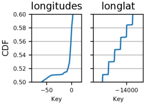
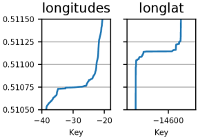
We run all experiments using 8-byte keys from some dataset and randomly generated fixed-size payloads. We evaluate ALEX on 4 datasets, whose characteristics and CDFs are shown in Table 1 and Fig. 8. The longitudes dataset consists of the longitudes of locations around the world from Open Street Maps (AWS, [n.d.]). The longlat dataset consists of compound keys that combine longitudes and latitudes from Open Street Maps by applying the transformation $k=180\cdot\text{floor}(\text{longitude})+\text{latitude}$ to every pair of longitude and latitude. The resulting distribution of keys $k$ is highly non-linear. The lognormal dataset has values generated according to a lognormal distribution with $\mu=0$ and $\sigma=2$, multiplied by $10^{9}$ and rounded down to the nearest integer. The YCSB dataset has values representing user IDs generated according to the YCSB Benchmark (Cooper et al., 2010), which are uniformly distributed across the full 64-bit domain, and uses an 80-byte payload. These datasets do not contain duplicate values. Unless otherwise stated, these datasets are randomly shuffled to simulate a uniform dataset distribution over time.

(a)

(b)

(c)

Figure 8. Dataset CDFs, and zoomed-in CDFs.

Table 1. Dataset Characteristics

	longitudes	longlat	lognormal	YCSB
Num keys	1B	200M	190M	200M
Key type	double	double	64-bit int	64-bit int
Payload size	8B	8B	8B	80B
Total size	16GB	3.2GB	3.04GB	17.6GB

(a)

(b)

(c)

(d)

(e)

(f)

(g)

(h)

(i)

(j)

Figure 9. ALEX vs. Baselines: Throughput & Index Size. Throughput includes model retraining time.

6.1.2. Workloads

Our primary metric for evaluating ALEX is average throughput. We evaluate throughput for five workloads: (1) a read-only workload, (2) a read-heavy workload with 95% reads and 5% inserts, (3) a write-heavy workload with 50% reads and 50% inserts, (4) a short range query workload with 95% reads and 5% inserts, and (5) a write-only workload, to complete the read-write spectrum. For the first three workloads, reads consist of a lookup of a single key. For the short range workload, a read consists of a key lookup followed by a scan of the subsequent keys. The number of keys to scan is selected randomly from a uniform distribution with a maximum scan length of 100. For all workloads, keys to look up are selected randomly from the set of existing keys in the index according to a Zipfian distribution. The first four workloads roughly correspond to Workloads C, B, A, and E from the YCSB benchmark (Cooper et al., 2010), respectively. For a given dataset, we initialize an index with 100 million keys. We then run the workload for 60 seconds, inserting the remaining keys. We report the throughput of operations completed in that time, where operations are either inserts or reads. For the read-write workloads, we interleave the operations: for the read-heavy workload and short range workload, we perform 19 reads/scans, then 1 insert, then repeat the cycle; for the write-heavy workload, we perform 1 read, then 1 insert, then repeat the cycle.

Table 2. ALEX Statistics after Bulk Load

	longitudes	longlat	lognormal	YCSB
Avg depth	1.01	1.56	1.80	1
Max depth	2	4	3	1
Num inner nodes	55	1718	24	1
Num data nodes	4450	23257	757	1024
Min DN size	672B	16B	224B	12.3MB
Median DN size	161KB	39.6KB	2.99MB	12.3MB
Max DN size	5.78MB	8.22MB	14.1MB	12.3MB

6.2. Overall Results

6.2.1. Read-only Workloads

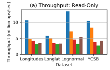
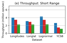
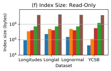
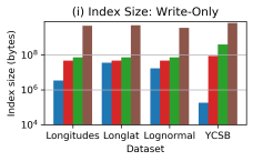
For read-only workloads, Figs. 9a and 9f show that ALEX achieves up to 4.1$\times$, 2.2$\times$, 2.9$\times$, 3.0$\times$ higher throughput and 800$\times$, 15$\times$, 160$\times$, 8000$\times$ smaller index size than the B+Tree, Learned Index, Model B+Tree, and ART, respectively.

On the longlat and YCSB datasets, ALEX performance is similar to Learned Index. The longlat dataset is highly non-uniform, so ALEX is unable to achieve high performance, even with adaptive RMI. The YCSB dataset is nearly uniform, so the optimal allocation of models is uniform; ALEX adaptively finds this optimal allocation, and Learned Index allocates this way by nature, so the resulting RMI structures are similar. On the other two datasets, ALEX has more performance advantage over Learned Index, which we explain in Section 6.3.

In general, Model B+Tree outperforms B+Tree while also having smaller index size, because the tuned page size of Model B+Tree is always larger than those of B+Tree. The benefit of models in Model B+Tree is greatest when the key distribution within each node is more uniform, which is why Model B+Tree has least benefit on non-uniform datasets like longlat.

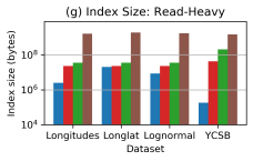
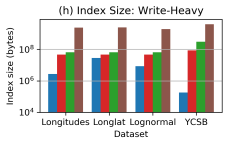
The index size of ALEX is dependent on how well ALEX can model the data distribution. On the YCSB dataset, ALEX does not require a large RMI to accurately model the distribution, so ALEX achieves small index size. However, on datasets that are more challenging to model such as longlat, ALEX has a larger RMI with more nodes. ALEX has smaller index size than the Learned Index, even when throughput is similar, for two reasons. First, ALEX uses model-based inserts to obtain better predictive accuracy for each model, which we show in Section 6.3, and therefore achieves high throughput while using relatively fewer models. Second, ALEX adaptively allocates data nodes to different parts of the key space and does not use any more models than necessary (Fig. 3), whereas Learned Index fixes the number of models and ends up with many redundant models. The index size of ART is higher than all other indexes. (Leis et al., 2013) claims that ART uses between 8 and 52 bytes to store each key, which is in agreement with the observed index sizes.

Table 2 shows ALEX statistics after bulk loading, including data node (DN) sizes. The root has depth 0. Average depth is averaged over keys. The max depth of the tuned B+Tree is 4 on the YCSB dataset and 5 on the other datasets. Datasets that are easier to model result in fewer nodes. For uniform datasets like YCSB, the data node sizes are also uniform.

6.2.2. Read-Write Workloads

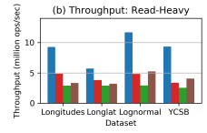
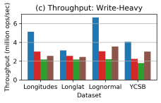
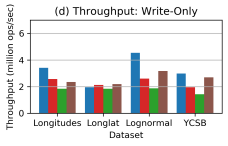
For read-write workloads, Figs. 9b, 9c, 9d, 9g, 9h and 9i show that ALEX achieves up to 4.0$\times$, 2.7$\times$, 2.7$\times$ higher throughput and 2000$\times$, 475$\times$, 36000$\times$ smaller index size than the B+Tree, Model B+Tree, and ART, respectively. The Learned Index has insert time orders of magnitude slower than ALEX and B+Tree, so we do not include it in these benchmarks.

The relative performance advantage of ALEX over baselines decreases as the workload skews more towards writes, because all indexes must pay the cost of copying when splitting/expanding nodes. Copying has an especially big impact for YCSB, for which payloads are 80 bytes. ART achieves comparable throughput to ALEX on the write-only workload for YCSB because ART does not keep payloads clustered, so it avoids the high cost of copying 80-byte payloads. Note that ALEX could similarly avoid copying large payloads by storing unclustered payloads separately and keeping a pointer with every key; however, this would impact scan performance. On datasets that are challenging to model such as longlat, ALEX only achieves comparable write-only throughput to Model B+Tree and ART, but is still faster than B+Tree.

6.2.3. Range Query Workloads

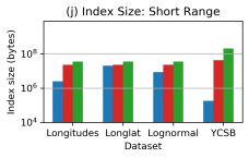
Figs. 9e and 9j show that ALEX maintains its advantage over B+Tree on the short range workload, achieving up to 2.27$\times$, 1.77$\times$ higher throughput and 1000$\times$, 230$\times$ smaller index size than B+Tree and Model B+Tree, respectively. However, the relative throughput benefit decreases, compared to Fig. 9b. This is because as scan time begins to dominate overall query time, the speedups that ALEX achieves on lookups become less apparent. The ART implementation from (Dadgar, [n.d.]) does not support range queries; we suspect range queries on ART would be slower than for the other indexes because ART does not cluster payloads, leading to poor scan locality. Section C.2 shows that ALEX continues to outperform other indexes on a workload that mixes inserts, point lookups, and short range queries.

(a)

(b)

Figure 10. (a) When scan length exceeds 1000 keys, ALEX is slower on range queries than a B+Tree whose page size is re-tuned for different scan lengths. (b) However, throughput of the re-tuned B+Tree suffers for other operations, such as point lookups and inserts in the write-heavy workload.

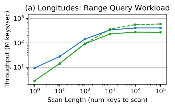
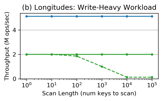
To show how performance varies with range query selectivity, we compare ALEX against two B+Tree configurations with increasingly larger range scan length over the longitudes dataset (Fig. 10a). In the first B+Tree configuration, we use the optimal B+Tree page size on the write-heavy workload (Fig. 9c), which is 1KB (solid green line). In the second B+Tree configuration, we tune the B+Tree page size for each different scan length (dashed green line).

Unsurprisingly, Fig. 10a shows as scan length increases, the throughput in terms of keys scanned per second increases for all indexes due to better locality and a smaller fraction of time spent on the initial point lookup. Furthermore, ALEX outperforms the 1KB-page B+Tree for all scan lengths due to ALEX’s larger nodes; median ALEX data node size is 161KB on the longitudes dataset (Table 2), which benefits scan locality—scanning larger contiguous chunks of memory leads to better prefetching and fewer pointer chases. This makes up for the Gapped Array’s overhead.

However, if we re-tune the B+Tree page size for each scan length (dashed green line), the B+Tree outperforms ALEX when scan length exceeds 1000 keys because past this point, the overhead of Gapped Array outpaces ALEX’s scan locality advantage from having larger node sizes. However, this comes at the cost of performance on other operations: Fig. 10b shows that if we run the re-tuned B+Tree on the write-heavy workload, which includes both point lookups and inserts, its performance would begin to decline when scan length exceeds 100 keys. In particular, larger B+Tree pages lead to a higher number of search iterations for lookups and shifts for inserts; ALEX avoids both of these problems for large data nodes by using Gapped Arrays with model-based inserts. We show in Section C.1 that this behavior also occurs on the other three datasets.

6.2.4. Bulk Loading

(a)

(b)

Figure 11. ALEX takes 50% more than time than B+Tree to bulk load on average, but quickly makes up for this by having higher throughput.

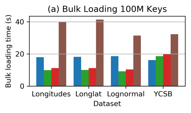
We compare the time to initialize each index with bulk loading, which includes the time to sort keys. Fig. 11a shows that on average, ALEX only takes 50% more time to bulk load than B+Tree, and in the worst case is only 2$\times$ slower than B+Tree. On the YCSB dataset, B+Tree and Model B+Tree take longer to bulk load due to the larger payload size, but bulk loading ALEX remains efficient due to its simple structure (Table 2). Model B+Tree is slightly slower to bulk load than B+Tree due to the overhead of training models for each node. ART is slower to bulk load than B+Tree, Model B+Tree, and ALEX.

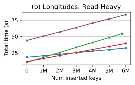
ALEX can quickly make up for its slower bulk loading time than B+Tree by having higher throughput performance. Fig. 11b shows that when running the read-heavy workload on the longitudes dataset, ALEX’s total time usage (bulk loading plus workload) drops below all other indexes after only 3 million inserts. We provide a more detailed bulk loading evaluation in Section A.

6.2.5. Scalability

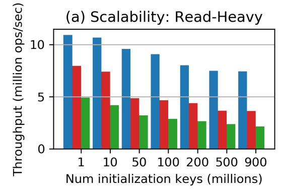
ALEX performance scales well to larger datasets. We again run the read-heavy workload on the longitudes dataset, but instead of initializing the index with 100 million keys, we vary the number of initialization keys. Fig. 12a shows that as the number of indexed keys increases, ALEX maintains higher throughput than B+Tree and Model B+Tree. In fact, as dataset size increases, ALEX throughput decreases at a surprisingly slow rate. This occurs because ALEX adapts its RMI structure in response to the incoming data.

(a)

(b)

(c)

Figure 12. ALEX maintains high throughput when scaling to large datasets and under data distribution shifts. (RH = Read-Heavy, WH = Write-Heavy)

6.2.6. Dataset Distribution Shift

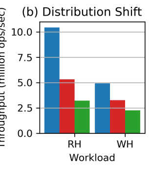
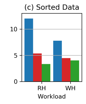
ALEX is robust to dataset distribution shift. We initialize the index with the 50 million smallest keys and run read-write workloads by inserting the remaining keys in random order. This simulates distribution shift because the keys we initialize with come from a completely disjoint domain than the keys we subsequently insert with. Fig. 12b shows that ALEX maintains up to 3.2$\times$ higher throughput than B+Tree in this scenario. ALEX is also robust to adversarial patterns such as sequential inserts in sorted order, in which new keys are always larger than the maximum key currently indexed. Fig. 12c shows that when we initialize with the 50 million smallest keys and insert the remaining keys in ascending sorted order, ALEX has up to $3.6\times$ higher throughput than B+Tree. Section B further shows that ALEX is robust to radically changing key distributions.

Figure 13. Impact of Gapped Array and adaptive RMI.

(a)

(b)

(c)

Figure 14. ALEX achieves smaller prediction error than the Learned Index.

6.3. Drilldown into ALEX Design Trade-offs

In this section, we delve deeper into how node layout and adaptive RMI help ALEX achieve its design goals.

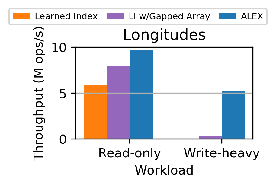
Part of ALEX’s advantage over Learned Index comes from using model-based insertion with Gapped Arrays in the data nodes, but most of ALEX’s advantage for dynamic workloads comes from the adaptive RMI. To demonstrate the effects of each contribution, Fig. 14 shows that taking a 2-layer Learned Index and replacing the single dense array of values with a Gapped Array per leaf (LI w/Gapped Array) already achieves significant speedup over Learned Index for the read-only workload. However, a Learned Index with Gapped Arrays achieves poor performance on read-write workloads due to the presence of fully-packed regions which require shifting many keys for each insert. ALEX’s ability to adapt the RMI structure to the data is necessary for good insert performance.

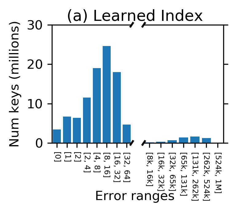
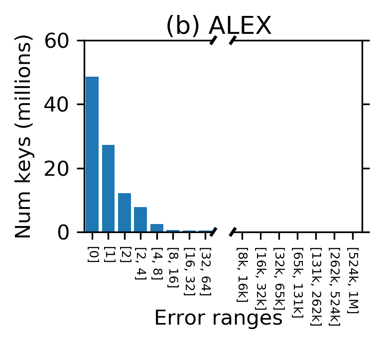
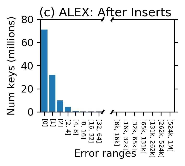
During lookups, the majority of the time is spent doing local search around the predicted position. Smaller prediction errors directly contribute to decreased lookup time. To analyze the prediction errors of the Learned Index and ALEX, we initialize an index with 100 million keys from the longitudes dataset, use the index to predict the position of each of the 100 million keys, and track the distance between the predicted position and the actual position. Fig. 14a shows that the Learned Index has prediction error with mode around 8-32 positions, with a long tail to the right. On the other hand, ALEX achieves much lower prediction error by using model-based inserts. Fig. 14b shows that after initializing, ALEX often has no prediction error, the errors that do occur are often small, and the long tail of errors has disappeared. Fig. 14c shows that even after 20 million inserts, ALEX maintains low prediction errors.

Table 3. Data Node Actions When Full (Write-Heavy)

	longitudes	longlat	lognormal	YCSB
Expand + scale	26157	113801	2383	1022
Expand + retrain	219	2520	2	1026
Split sideways	79	2153	7	0
Split downwards	0	230	0	0
Total times full	26455	118704	2392	2048

Once a data node becomes full, one of four actions happens: if there is no cost deviation, then (1) the node is expanded and the model is scaled. Otherwise, the node is either (2) expanded and its model retrained, (3) split sideways, or (4) split downwards. Table 3 shows that in the vast majority of cases, the data node is simply expanded and the model scaled, which implies that models usually remain accurate even after inserts, assuming no radical distribution shift. The number of occurrences of a data node becoming full is correlated with the number of data nodes (Table 2). On YCSB, expansion with model retraining is more common because the data nodes are large, so cost deviation often results simply from randomness.

Figure 15. Latency of a single operation.

Figure 16. Exponential vs. other search methods.

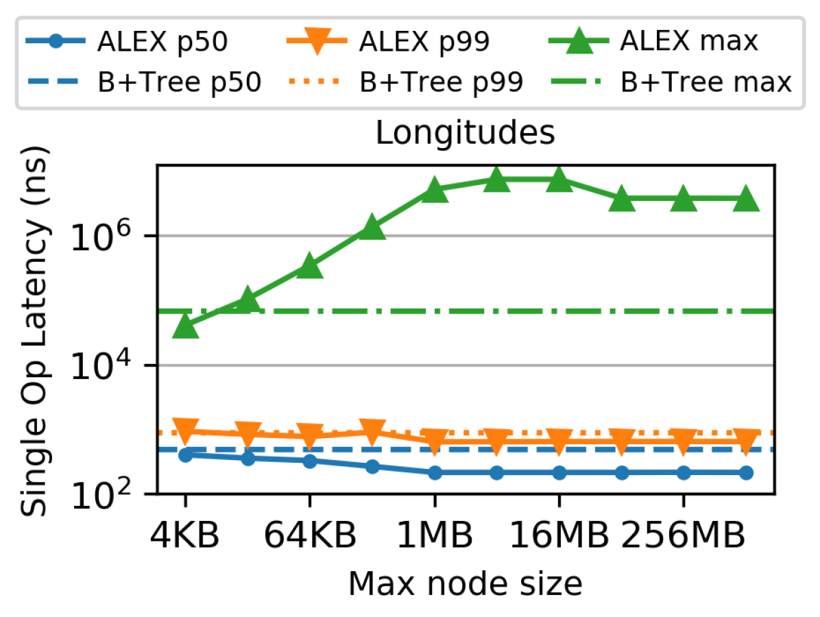
Users can adjust the max node size to achieve target tail latencies, if desired. In Fig. 16, we run the write-heavy workload on the longitudes dataset, measuring the latency for every operation. As we increase the max node size, median and even p99 latency of ALEX decreases, because ALEX has more flexibility to build a better-performing RMI (e.g., ability to have higher internal node fanout). However, maximum latency increases, because an insert that triggers an expansion or split of a large node is slow. If the user has strict latency requirements, they can decrease the max node size accordingly. After increasing the max node size beyond 64MB, latencies do not change because ALEX never decides to use a node larger than 64MB.

6.3.1. Search Method Comparison

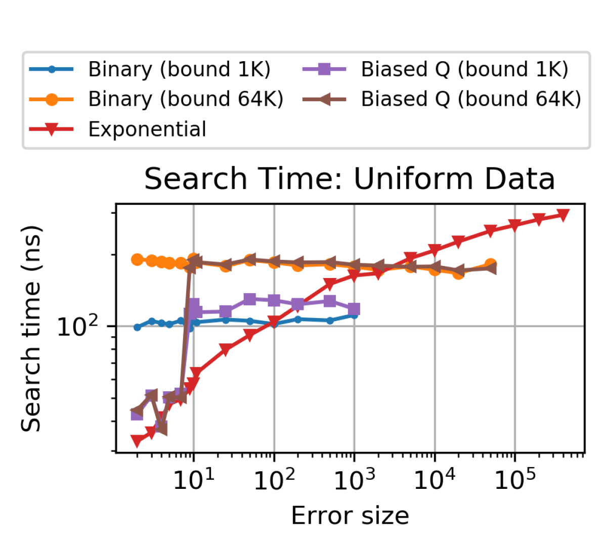
In order to show the trade-off between exponential search and other search methods, we perform a microbenchmark on synthetic data. We create a dataset with 100 million perfectly uniformly distributed doubles. We then perform searches for 10 million randomly selected values from this dataset. We use three search methods: binary search and biased quaternary search (proposed in (Kraska et al., 2018) to take advantage of accurate predictions), each evaluated with two different error bound sizes, as well as exponential search. For each lookup, the search method is given a predicted position that has some synthetic amount of error in the distance to the actual position value. Fig. 16 shows that the search time of exponential search increases proportionally with the logarithm of error size, whereas the binary search methods take a constant amount of time, regardless of error size. This is because binary search must always begin search within its error bounds, and cannot take advantage of cases when the error is small. Therefore, exponential search should outperform binary search if the prediction error of the RMI models in ALEX is small. As we showed in Section 6.3, ALEX maintains low prediction errors through model-based inserts. Therefore, ALEX is well suited to take advantage of exponential search. Biased quaternary search is competitive with exponential search when error is below $\sigma$ (we set $\sigma=8$ for this experiment; see (Kraska et al., 2018) for details) because search can be confined to a small range, but performs similarly to binary search when error exceeds $\sigma$ because the full error bound must be searched. We prefer exponential search to biased quaternary search due to its smoother performance degradation and simplicity of implementation (e.g., no need to tune $\sigma$).

7. Related Work

Learned Index Structures: The most relevant work is the Learned Index (Kraska et al., 2018), discussed in Section 2.2. Learned Index has similarities to prior work that explored how to compute down a tree index. Tries (Knuth, 1998) use key prefixes instead of B+Tree splitters. Masstree (Mao et al., 2012) and Adaptive Radix Tree (Leis et al., 2013) combine the ideas of B+Tree and trie to reduce cache misses. Plop-hashing (Kriegel and Seeger, 1988) uses piecewise linear order-preserving hashing to distribute keys more evenly over pages. Digital B-tree (Lomet, 1981) uses bits of a key to compute down the tree more flexibly.  (Lomet, 1987) proposes to partially expand the space instead of always doubling when splitting in B+Tree.  (Graefe, 2006) proposes the idea of interpolation search within B+Tree nodes; this idea was revisited in (Neumann, 2017). The interpolation-based search algorithms in (Van Sandt et al., 2019) can complement ALEX’s search strategy. Hermit (Wu et al., 2019) creates a succinct tree structure for secondary indexes.

Other works propose replacing the leaf nodes of a B+Tree with other data structures in order to compress the index, while maintaining search and update performance. FITing-tree (Galakatos et al., 2019) uses linear models in its leaf nodes, while BF-tree (Athanassoulis and Ailamaki, 2014) uses bloom filters in its leaf nodes.

All these works share the idea that using extra computation or data structures can make search faster by reducing the number of binary search hops and corresponding cache misses, while allowing larger node sizes and hence a smaller index size. However, ALEX is different in several ways: (1) We use a model to split the key space, similar to a trie, but no search is required until we reach the leaf level. (2) ALEX’s accurate linear models enable larger node sizes without sacrificing search and update performance. (3) Model-based insertion reduces the impact of model’s misprediction. (4) ALEX’s cost models automatically adjust the index structure to dynamic workloads.

Memory Optimized Indexes: There is a large body of work on optimizing tree index structures for main memory by exploiting hardware features such as CPU cache, multi-core, SIMD, and prefetching. CSS-trees (Rao and Ross, 1999) improve B+Tree’s cache behavior by matching index node size to CPU cache-line size and eliminating pointers in index nodes by using arithmetic operations to find child nodes. CSB⁺-tree (Rao and Ross, 2000) extends the static CSS-trees by supporting incremental updates without sacrificing CPU cache performance. (Hankins and Patel, 2003) evaluates the effect of node size on the performance of CSB⁺-tree analytically and empirically. pB+-tree (Chen et al., 2001) uses larger index nodes and relies on prefetching instructions to bring index nodes into cache before nodes are accessed. In addition to optimizing for cache performance, FAST (Kim et al., 2010) further optimizes searches within index nodes by exploiting SIMD parallelism.

ML in other DB components: Machine learning has been used to improve cardinality estimation (Kipf et al., 2018; Dutt et al., 2019), query optimization (Marcus et al., 2019), workload forecasting (Ma et al., 2018), multi-dimensional indexing (Nathan et al., 2020), and data partitioning (Yang et al., 2020). SageDB (Kraska et al., 2019) envisions a database system in which every component is replaced by a learned component. These studies show that the use of machine learning enables workload-specific optimizations, which also inspired our work.

8. Conclusion

We build on the excitement of learned indexes by proposing ALEX, a new updatable learned index that effectively combines the core insights from the Learned Index with proven storage and indexing techniques. Specifically, we propose a Gapped Array node layout that uses model-based inserts and exponential search, combined with an adaptive RMI structure driven by simple cost models, to achieve high performance and low memory footprint on dynamic workloads. Our in-depth experimental results show that ALEX not only consistently beats B+Tree across the read-write workload spectrum, it even beats the existing Learned Index, on all datasets, by up to 2.2$\times$ with read-only workloads.

We believe this paper presents important learnings to our community and opens avenues for future research in this area. We intend to pursue open theoretical problems about ALEX performance, supporting secondary storage for larger than memory datasets, and new concurrency control techniques tailored to the ALEX design.

Acknowledgements. This research is supported by Google, Intel, and Microsoft as part of the MIT Data Systems and AI Lab (DSAIL) at MIT, NSF IIS 1900933, DARPA Award 16-43-D3M-FP040, and the MIT Air Force Artificial Intelligence Innovation Accelerator (AIIA).

A. Extended Bulk Loading Evaluation

In this section, we provide an extended version of Section 6.2.4, which evaluates the speed of ALEX’s bulk loading mechanism against other indexes. ALEX uses two optimizations for bulk loading—approximate model computation (AMC) and approximate cost computation (ACC)—which we explain in more detail below.

Figure 17. With both optimizations (AMC and ACC), ALEX only takes 50% more than time than B+Tree to bulk load when averaged across four datasets.

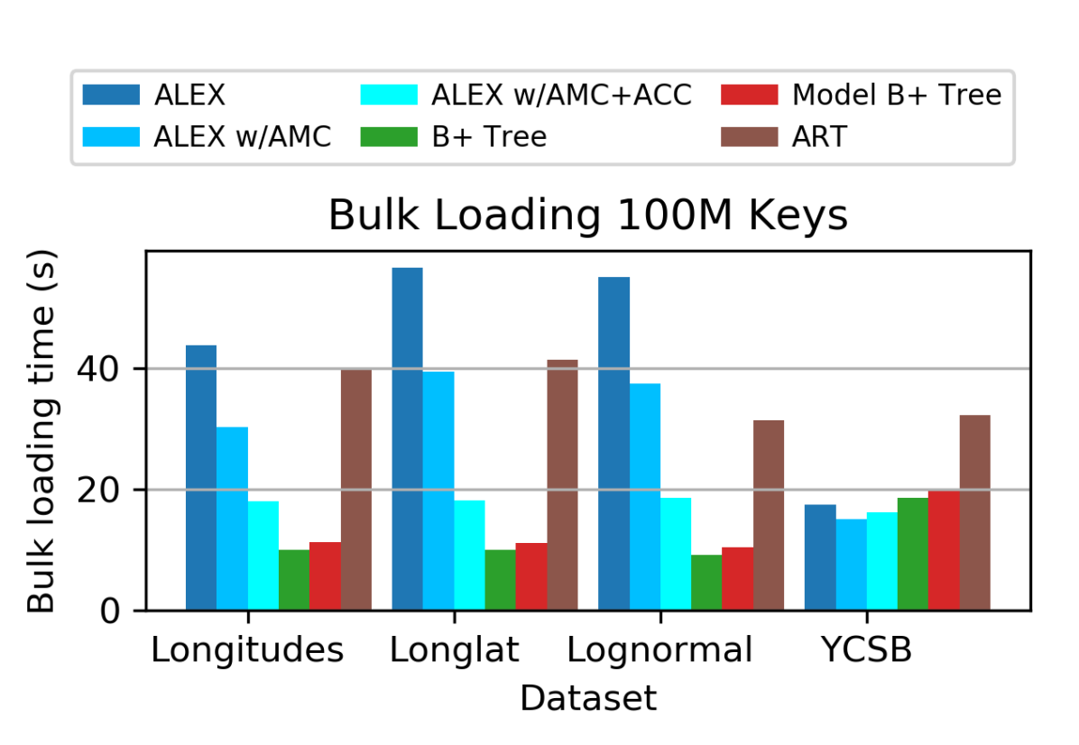
For each index, we bulk load 100 million keys from each of the four datasets from Section 6. This includes the time used to sort the 100 million keys. Fig. 17, which is a more detailed version of Fig. 11a, shows that on average, ALEX with no optimizations takes 3.6$\times$ more time to bulk load than B+Tree, which is the fastest index to bulk load. However, with the AMC optimization, ALEX takes 2.6$\times$ more time on average than B+Tree. With both optimizations, ALEX only takes 50% more than time on average than B+Tree, and in the worst case is only 2$\times$ slower than B+Tree. The results for ALEX in Section 6.2.4 use both optimizations. On the YCSB dataset, ALEX’s structure is very simple (Table 2), and therefore is very efficient to bulk load even when unoptimized; in fact, ALEX’s large node sizes allow ALEX to bulk load faster than other indexes due to the benefits of locality.

(a)

(b)

Figure 18. Using the AMC optimization when bulk loading does not cause any noticeable change in ALEX performance, but ACC can cause a slight decrease in throughput for write-heavy workloads.

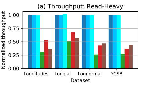
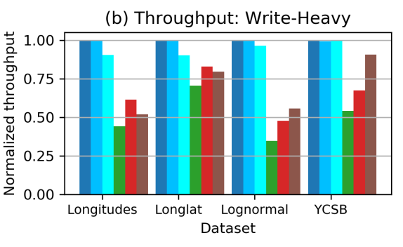
Fig. 18 shows the impact of the two optimizations on the throughput of running a read-heavy or write-heavy workload on ALEX after bulk loading. The AMC optimization has negligible impact on throughput for all datasets and for both workloads. Adding the ACC optimization has negligible impact on the read-heavy workload, but decreases throughput by up to 9.6% on the write-heavy workload; we provide explanation for this behavior below.

Based on these results, we conclude that the AMC optimization should always be used to improve bulk loading performance, whereas the ACC optimization might cause a slight decrease in throughput performance and therefore should be used only if faster bulk loading is required. We now explain the two optimizations in more detail.

A.1. Approximate Model Computation

We perform approximate model computation (AMC) efficiently while achieving accuracy through progressive systematic sampling. Given a data node of sorted keys, we perform systematic sampling (i.e., sampling every $n$th key) to obtain a small sample of keys, and compute a linear regression model using that sample. We then repeatedly double the sample size and recompute the linear model using the larger sample. When the relative change in the model parameters (i.e., the slope and intercept) both change by less than 1% from one sample to the next, we terminate the process. In our experience, this 1% threshold strikes a balance between achieving accuracy and using small sample sizes, and did not need to be tuned.

Note that by using systematic sampling, all keys in the sample used to compute the current model will also appear in all subsequent samples. Therefore, each linear model can be computed progressively starting from the existing model computed from the previous sample, instead of from scratch. No redundant work is done, and even in the worst case, AMC will take no more time than computing one linear model from all keys (if we ignore minor overheads and the effects of locality).

A.2. Approximate Cost Computation

We also perform approximate intra-node cost computation (ACC) for a data node of sorted keys through progressive systematic sampling. However, ACC differs from AMC in two ways. First, the cost for a data node must be computed from scratch for each sample; the cost depends on where keys are placed within a Gapped Array, which itself depends on which keys are present in the sample. Second, and more importantly, the cost of a data node naturally increases with the number of keys in the node. This makes ACC an extrapolation problem (i.e., use the cost of a small sample to predict the cost of the entire data node), whereas AMC is an estimation problem (i.e., use a small sample to directly estimate the model parameters).

ACC repeatedly doubles its sample size. Let the latest three samples be $s_{1}$, which is half the size of $s_{2}$, which is half the size of $s_{3}$. Let the costs computed from these samples be $c_{1}$, $c_{2}$, and $c_{3}$, respectively. We use the $c_{1}$ and $c_{2}$ to perform a linear extrapolation to predict $c_{3}$. If this prediction is accurate (i.e., if relative error with the true $c_{3}$ is within 20%), then we use $c_{2}$ and $c_{3}$ to perform a linear extrapolation to predict the cost of the entire data node, and we terminate the process. Otherwise, we continue doubling the sample size. The intuition behind this process is that we want to verify the accuracy of extrapolation using small samples before extrapolating to the entire data node. We allow a higher relative error than for AMC because the extrapolation process is inherently imprecise, since it is impossible to accurately predict the cost using a sample without a priori knowledge of the data distribution.

We can now explain why Fig. 18 shows that adding the ACC optimization decreases throughput on the write-heavy workload by up to 9.6%. It is because the average number of shifts per insert, which is one component of the intra-node cost, is difficult to estimate accurately. Therefore, if ACC underestimates the component of cost related to shifts, the bulk loaded ALEX structure may be inefficient for inserts (e.g., an insert that requires more shifts than expected can be very slow). The intra-node cost is more difficult to approximate accurately for the longitudes and longlat datasets, which is why the decrease in throughput is most noticeable for those two datasets. However, note that over time, the dynamic nature of ALEX will eventually correct for incorrectly estimated costs, so throughput performance in the long run will be independent of the bulk loading mechanism.

B. Extreme Distribution Shift Evaluation

In order to evaluate the performance of ALEX under a radically changing key distribution, we combine the four datasets from Section 6 into one dataset by randomly selecting 50 million keys from each of the four datasets in order to create one combined dataset with 200 million keys. We scaled keys from each dataset to fit in the same domain. Note that we would not typically expect a single table to contain keys from four independent distributions. Therefore, this complex combined dataset is an extreme stress test for the adaptibility of ALEX.

We run a write-heavy workload (50% point lookups and 50% inserts) over the combined dataset, but we vary the order in which keys are bulk loaded and inserted. For all variants, we bulk load using 50 million keys and run the write-heavy workload until the remaining 150 million keys are all inserted. We create four variants that represent distribution shift; each variant bulk loads using the 50 million keys selected from one of the four original datasets, then gradually inserts keys from the other three original datasets, in order. For example, the “L-LN-LL-Y” variant bulk loads using the 50 million keys selected from the longitudes (L) dataset, then runs the write-heavy workload by inserting the 50 million keys from the lognormal (LN) dataset, then the longlat (LL) dataset, and finally the YCSB (Y) dataset. For reference, we also include a variant in which all 200 million keys are shuffled, so that no key distribution shift is observed.

Figure 19. ALEX maintains high performance under radically changing key distribution, although performance does differ slightly depending on the distribution used for bulk loading.

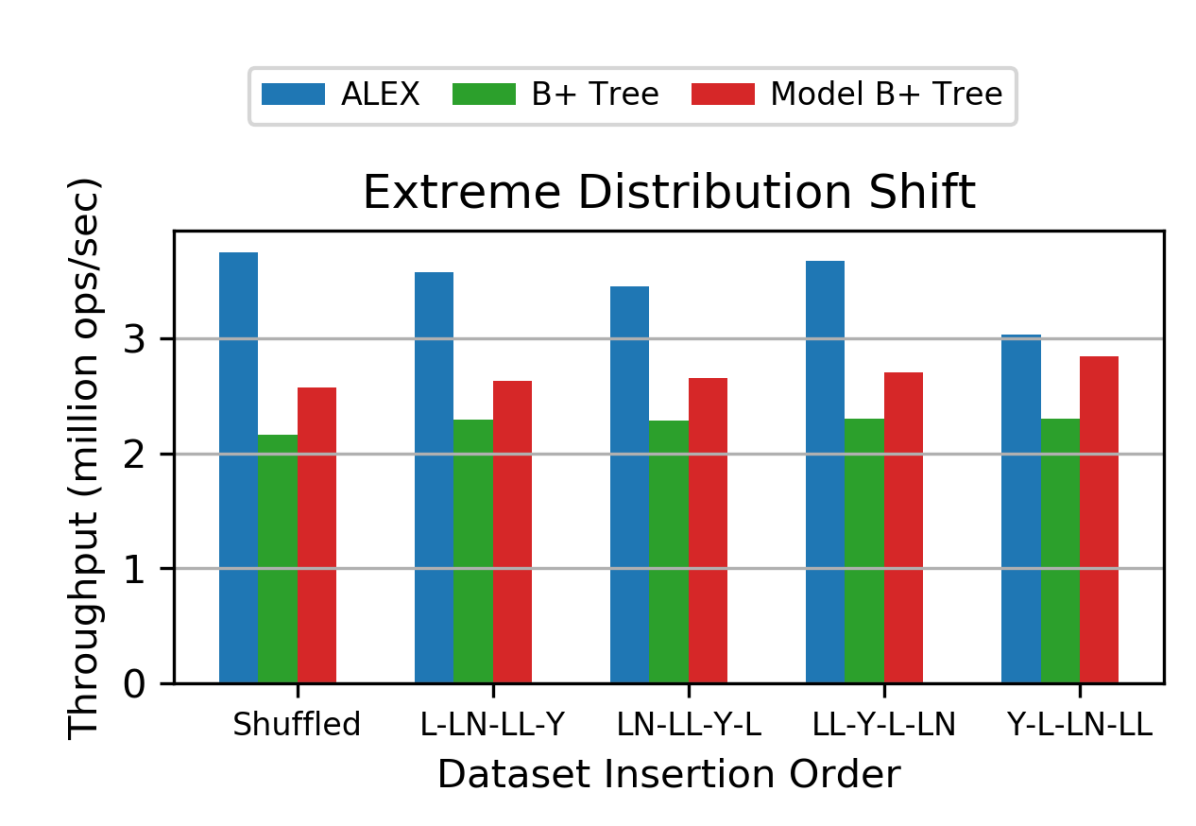
Fig. 19 provides three insights. First, on the workload that represents no distribution shift (“Shuffled”), ALEX continues to outperform other indexes. It is interesting to note that the throughput of ALEX on the combined dataset is between the throughputs achieved on each dataset individually (Fig. 9c): higher than for longlat, and lower than for the other three datasets. Second, ALEX achieves lower throughput in the four variants that represent distribution shift than without distribution shift, but still outperforms other indexes. This result aligns with the intuition that ALEX must spend extra time restructuring itself to adapt to the changing key distribution. Third, the throughput differs based on which dataset’s keys are used to bulk load ALEX. When bulk loading using keys from a complex key distribution, such as longlat, ALEX achieves throughput similar to the variant with no distribution shift; on the other hand, when bulk loading using keys from a simple key distribution, such as YCSB, ALEX throughput suffers. This is because when bulk loading with a simple key distribution, the bulk loaded structure of ALEX will be shallow, with few nodes (Table 2). When the subsequently inserted keys come from a much more complex key distribution, ALEX must quickly adapt its structure to be deeper and have more nodes, which can incur significant overhead. On the other hand, when bulk loading with a complex key distribution, the bulk loaded structure is already deep, with many nodes, and so can more readily adapt to changes in the key distribution without too much overhead.

To allow ALEX to more quickly adapt the RMI structure to radically changing key distributions: (1) we check data nodes periodically for cost deviation instead of only when the data node is full, and (2) if the number of shifts per insert in a data node is extremely high, we force the data node to split (as opposed to expanding and retraining the model). When no distribution shift occurs, these two checks have negligible impact on performance, because checking for cost deviation has minimal overhead and cost deviation occurs infrequently (Table 3). By default, we check for cost deviation for every 64 inserts into that data node, and over 100 shifts per insert is considered extremely high.

C. Extended Range Query Evaluation

(a)

(b)

(c)

(d)

(e)

(f)

(g)

(h)

Figure 20. Across all datasets, ALEX maintains an advantage over fixed-page-size B+Tree even for longer range scans.

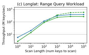
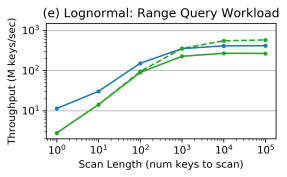
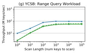
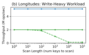
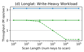
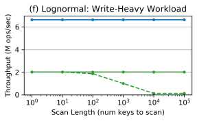
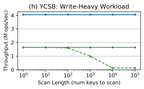
C.1. Varying Range Query Scan Length

We extend the experiment from Fig. 10 to all four datasets. Fig. 20 shows that across all datasets, ALEX maintains its advantage over fixed-page-size B+Tree, and re-tuning the B+Tree page size can lead to better range query performance but will decrease performance on point lookups and inserts. For both ALEX and B+Tree, performance on YCSB is slower than for the other three datasets because YCSB has a larger payload size, which worsens scan locality.

C.2. Mixed Workload Evaluation

(a)

Figure 21. ALEX maintains high performance under a mixed workload with 5% inserts, 85% point lookups, and 10% short range queries.

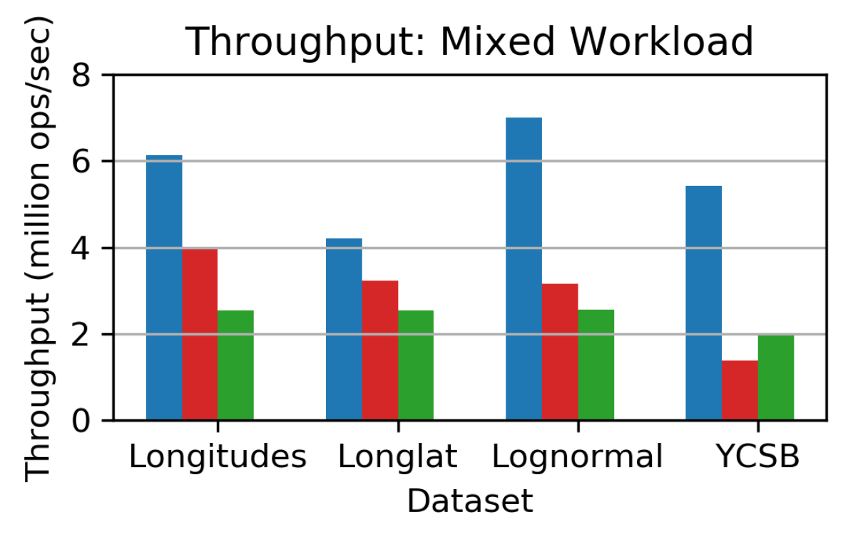
We evaluate a mixed workload with 5% inserts, 85% point lookups, and 10% range queries with a maximum scan length of 100. The remainder of the experimental setup is the same as in Section 6.1. Fig. 21 shows that ALEX maintains its performance advantage over other indexes. The ART implementation from (Dadgar, [n.d.]) does not support range queries.

D. Drilldown into Cost Computation

In this section, we first provide more details about the cost model introduced in Section 4.3.4. We then evaluate the performance of computing costs using cost models.

Table 4. Terms used to describe the cost model

Term	Description
$\mathcal{A}$	An instantiation of ALEX
$\mathcal{N}$	Set of all nodes in $\mathcal{A}$
$\mathcal{D}$	Set of data nodes in $\mathcal{A}$. This means that $\mathcal{D}\subseteq\mathcal{N}$
$S(N)$	Average number of exponential search iterations for a lookup in $N\in\mathcal{D}$
$I(N)$	Average number of shifts for an insert into $N\in\mathcal{D}$
$K(N)$	Number of keys in $N\in\mathcal{D}$
$F(N)$	Fraction of operations that are inserts (as opposed to lookups) in $N\in\mathcal{D}$
$C_{I}(N)$	Intra-node cost of $N\in\mathcal{D}$
$C_{T}(N)$	TraverseToLeaf cost of $N\in\mathcal{D}$
$D(N)$	Depth of $N\in\mathcal{N}$ (root node has depth 0)
$B(\mathcal{A})$	Total size in bytes of all nodes in $\mathcal{A}$
$w_{s},w_{i},w_{d},w_{b}$	Fixed pre-defined weight parameters

D.1. Cost Model Details

We formally define the cost model using the terms in Table 4. At a high level, the intra-node cost of a data node represents the average time to perform an operation (i.e., a point lookup or insert) on that data node, and the TraverseToLeaf cost of a data node represents the time for traversing from the root node to the data node.

For a given data node $N\in\mathcal{D}$, the intra-node cost $C_{I}(N)$ is defined as

(1) $$C_{I}(N)=w_{s}S(N)+w_{i}I(N)F(N)$$

Both lookups and inserts must perform an exponential search, whereas only inserts must perform shifts. This is why $I(N)$ is weighted by $F(N)$.

For a given data node $N\in\mathcal{D}$, the TraverseToLeaf cost $C_{T}(N)$ of traversing from the root node to $N$ is defined as

(2) $$C_{T}(N)=w_{d}D(N)+w_{b}B(\mathcal{A})$$

The depth of $N$ is the number of pointer chases needed to reach the data node. In our cost model, every traverse to leaf has a fixed cost that is caused by the total size of the ALEX RMI, because larger RMI causes worse cache locality.

For an instantiation of ALEX $\mathcal{A}$, the cost of $\mathcal{A}$ represents the average time to perform a query (i.e., a point lookup or insert) starting from the root node, and is defined as

(3) $$C(\mathcal{A})=\frac{\sum_{N\in\mathcal{D}}(C_{I}(N)+C_{T}(N))K(N)}{\sum_{N\in\mathcal{D}}K(N)}$$

In other words, the cost of $\mathcal{A}$ is the sum of the intra-node cost and TraverseToLeaf cost of each data node, normalized by how many keys are contained in the data node. We normalize because each data node does not contribute equally to average query time. For example, a data node that has high intra-node cost but is rarely queried might not have as much impact on average query time as a data node with lower intra-node cost that is frequently queried. We use the number of keys in each data node as a proxy for its impact on the average query time. An alternative is to normalize using the true query access frequency of each data node.

The weight parameters $w_{s},w_{i},w_{d},w_{b}$ do not need to be tuned for each dataset or workload, because they represent fixed quantities. For our evaluation, we set $w_{s}=10$,$w_{i}=1$,$w_{d}=10$, and $w_{b}=10^{-6}$. In terms of impact on throughput performance, these weights intuitively mean that each exponential search iteration takes 10 ns, each shift takes 1 ns, each pointer chase to traverse down one level of the RMI takes 10 ns, and each MB of total size contributes a slowdown of 1 ns due to worse cache locality. As a side effect, $w_{b}$ acts as a regularizer to prevent the RMI from growing unnecessarily large. We found that our simple cost model performed well throughout our evaluation. However, it may still be beneficial to formulate a more complex cost model that more accurately reflects true runtime; this is left as future work.

D.2. Cost Computation Performance

The cost of the entire RMI, $C(\mathcal{A})$, is never explicitly computed. Instead, all decisions based on cost are made locally. This is possible due to the linearity of the cost model. For example, when deciding between expanding a data node and splitting the data node in two, we compare the incremental impact on $C(\mathcal{A})$ between the two options. This only involves computing the intra-node cost of the expanded data node and each of the two split data nodes; the intra-node costs of all other data nodes in the RMI remain the same.

Cost computation occurs at two points during ALEX operation (Section 4.3.5): (1) when a data node becomes full, the expected intra-node cost is compared to the empirical intra-node cost to check for cost deviation. This comparison has very low performance overhead because the empirical values of $S(N)$ and $I(N)$ are maintained by the data node, so computing the empirical intra-node cost merely involves three multiplications and an addition. (2) If cost deviation is detected, ALEX must make a cost-based decision about how to adjust the RMI structure. This involves computing the expected intra-node cost of candidate data nodes which may be created as a result of adjusting the RMI structure. Since the candidate data nodes do not yet exist, we must compute the expected $S(N)$ and $I(N)$, which involves implicitly building the candidate data node. The majority of time spent on cost-based decision making is spent on computing expected $S(N)$ and $S(I)$.

Table 5. Fraction of time spent on cost computation

	longitudes	longlat	lognormal	YCSB
Read-Only	0	0	0	0
Read-Heavy	0.000271	0.000214	0.000617	0
Write-Heavy	0.00142	0.00901	0.00452	0.116
Write-Only	0.0270	0.0732	0.0237	0.149

Table 5 shows the fraction of overall workload time spent on computing costs and making cost-based decisions. On the read-only workload, no time is spent on cost-based decision because nodes never become full. As the fraction of writes increases, an increasing fraction of time is spent on cost computation because nodes become full more frequently. However, even on the write-only workload, cost computation takes up a small fraction of overall time spent on the workload. YCSB sees the highest fraction of time spent on cost computation, due to two factors: data nodes are larger, so computing $S(N)$ and $I(N)$ for larger candidate nodes takes more time, and lookups and inserts on YCSB are efficient, so data nodes become full more quickly. Longlat sees the next highest fraction of time spent on cost computation, which is due to the high frequency with which data nodes become full (Table 3).

E. Comparison of Gapped Array and PMA

The Gapped Array structure introduced in Section 3.2 has some similarities to an existing data structure known as the Packed Memory Array (PMA) (Bender and Hu, 2007). In this section, we first describe the PMA, and then we describe why we choose to not use the PMA within ALEX.

Like the Gapped Array, PMA is an array with gaps. Unlike the Gapped Array, PMA is designed to uniformly space its gaps between elements and to maintain this property as new elements are inserted. The PMA achieves this goal by rebalancing local portions of the array when the gaps are no longer uniformly spaced. Under random inserts from a static distribution, the PMA can insert elements in $O(\log{n})$ time, which is the same as the Gapped Array. However, when inserts do not come from a static distribution, the PMA can guarantee worst-case insertion in $O(\log^{2}{n})$ time, which is better than the worst case of the Gappd Array, which is $O(n)$ time.

We now describe the PMA more concretely; more details can be found in (Bender and Hu, 2007). The PMA is an array whose size is always a power of 2. The PMA divides itself into equally spaced segments, and the number of segments is also a power of 2. The PMA builds an implicit binary tree on top of the array, where each segment is a leaf node, each inner node represents the region of the array covered by its two children, and the root node represents the entire array. The PMA places density bounds on each node of this implicit binary tree, where the density bound determines the maximum ratio of elements to positions in the region of the array represented by the node. The nodes nearer the leaves will have higher density bounds, and the nodes nearer the root will have lower density bounds. The density bounds guarantee that no region of the array will become too packed. If an insertion into a segment will violate the segment’s density bounds, then we can find some local region of the array and uniformly redistribute all elements within this region, such that after the redistribution, none of the density bounds are violated. As the array becomes more full, ultimately no local redistribution can avoid violating density bounds. At this point, the PMA expands by doubling in size and inserting all elements uniformly spaced in the expanded array.

We do not use the PMA as the underlying storage structure for ALEX data nodes because the PMA negates the benefits of model-based inserts, which is critical for search performance. For example, when rebalancing a local portion of the array, the PMA spreads the keys in the local region over more space, which worsens search performance because the keys are moved further away from their predicted location. Furthermore, the main benefit of PMA—efficient inserts for non-static or complex key distributions—is already achieved by ALEX through the adaptive RMI structure. In our evaluation, we found that ALEX using data nodes built on Gapped Arrays consistently outperformed data nodes built on PMA.

F. Analysis of Model-based Search

Model-based inserts try to place keys in Gapped Array in their predicted positions. We analyze the trade-off between Gapped Array space usage and search performance in terms of ${c}$, the ratio of Gapped Array slots to number of actual keys. Assume the keys in the data node are $x_{1}<x_{2}<\cdots<x_{n}$, and the linear model before rounding is $y=ax+b$ when ${c}=1$, i.e., when no extra space is allocated. Define $\delta_{i}=x_{i+1}-x_{i},\Delta_{i}=x_{i+2}-x_{i}$. We first present a condition under which all the keys in that data node are placed in the predicted location, i.e., search for all keys are direct hits.

Theorem .1.

When ${c}\geq\frac{1}{a\min_{i=1}^{n-1}\delta_{i}}$, every key in the data node is placed in the predicted location exactly.

Proof.

Consider two keys in the leaf node $x_{i}$ and $x_{j},i\neq j$. The predicted locations before rounding are $y_{i}$ and $y_{j}$, respectively. When $|y_{i}-y_{j}|\geq 1$, we know that the rounded locations $\lfloor y_{i}\rfloor$ and $\lfloor y_{j}\rfloor$ cannot be equal. Under the linear model $y={c}(ax+b)$, we can write the condition as:

(4) $$|y_{i}-y_{j}|=|{c}a(x_{i}-x_{j})|\geq 1$$

If this condition is true for all the pairs $(i,j),i\neq j$, then all the keys will have a unique predicted location. For the condition Eq. (4) to be true for all $i\neq j$, it suffices to have:

(5) $$\min_{i=1}^{n-1}{c}a(x_{i+1}-x_{i})\geq 1$$

which is equivalent to ${c}\geq\frac{1}{a\min_{i=1}^{n-1}\delta_{i}}$. ∎

We now understand that $c=1$ corresponds to the optimal space, and $c\geq\frac{1}{a\min_{i=1}^{n-1}\delta_{i}}=c_{max}$ corresponds to the optimal search time (ignoring the effect of cache misses). We now bound the number of keys with direct hits when ${c}<c_{max}$.

Theorem .2.

The number of keys placed in the predicted location is no larger than $2+\left|\{1\leq i\leq n-2|\Delta_{i}>\frac{1}{ca}\}\right|$, where $\left|\{1\leq i\leq n-2|\Delta_{i}>\frac{1}{ca}\}\right|$ is the number of $\Delta_{i}$’s larger than $\frac{1}{ca}$.

Proof.

We define a mapping $f:[n-2]\rightarrow[n]$, where $f(i)$ is defined recursively according to the following cases:

Case (1): $y_{i+2}-y_{i}>1$. Let $f(i)=1$. Case (2): $y_{i+2}-y_{i}\leq 1,\lfloor y_{i+1}\rfloor=\lfloor y_{i}\rfloor,f(i-1)\leq i$ or $i=1$. Let $f(i)=i+1$. Case (3): Neither case (1) or (2) is true. Let $f(i)=i+2$.

We prove that $\forall 1\leq i<j\leq n-2$, if $f(i)>1,f(j)>1$, then $i+1\leq f(i)\leq i+2,j+1\leq f(j)\leq j+2$, and $f(i)<f(j)$.

First, when $f(i)>1,f(j)>1$, we know that case (1) is false for both $i$ and $j$. So $f(i)$ is either $i+1$ or $i+2$, and $f(j)$ is either $j+1$ or $j+2$.

Second, if $i+1<j$, then $f(i)\leq i+2<j+1\leq f(j)$. So we only need to prove $f(i)<f(j)$ when $i+1=j$. Now consider the only two possible values for $f(j)$, $j+1$ and $j+2$, when $i+1=j$. If $f(j)=j+1=i+2$, by definition we know that case (2) is true for $f(j)$. That means $f(j-1)=j$ or 1. But we already know $f(j-1)=f(i)>1$. So $f(i)=f(j-1)=j=i+1<i+2=f(j)$. If $f(j)=j+2$, then $f(i)\leq i+2<j+2=f(j)$.

So far, we have proved that $f(i)$ is unique when $f(i)>1$. Now we prove that the key $x_{f(i)}$ is not placed in $\lfloor y_{f(i)}\rfloor$ when $f(i)>1$, i.e., either case (2) or case (3) is true for $f(i)$. In both cases, $y_{i+2}-y_{i}\leq 1$, and the rounded integers $\lfloor y_{i+2}\rfloor$ and $\lfloor y_{i}\rfloor$ must be either equal or adjacent: $\lfloor y_{i+2}\rfloor-\lfloor y_{i}\rfloor\leq 1$. That means $\lfloor y_{i+1}\rfloor$ must be equal to either $\lfloor y_{i+2}\rfloor$ or $\lfloor y_{i}\rfloor$.

We prove by mathematical induction. For the minimal $i$ s.t. $f(i)>1$, if case (2) is true, $\lfloor y_{i+1}\rfloor=\lfloor y_{i}\rfloor$. That means $x_{i+1}$ cannot be placed at $\lfloor y_{i+1}\rfloor$ because that location is already occupied before $x_{i+1}$ is inserted. And $f(i)=i+1$ by definition. If case (2) is false, since we already know $y_{i+2}-y_{i}\leq 1$, $f(i-1)=1$ or $i=1$, it follows that $\lfloor y_{i+1}\rfloor>\lfloor y_{i}\rfloor$. That implies $\lfloor y_{i+1}\rfloor=\lfloor y_{i+2}\rfloor$. So $x_{i+2}$ cannot be placed at $\lfloor y_{i+2}\rfloor$. And $f(i)=i+2$ because case (3) happens.

Given that the key $x_{f(i-1)}$ is not placed at $\lfloor y_{f(i-1)}\rfloor$ when $f(i-1)>1$, we now prove it is also true for $i$. The proof for case (2) is the same as above. If case (2) is false, and $\lfloor y_{i+1}\rfloor>\lfloor y_{i}\rfloor$, the proof is also the same as above. The remaining possibility of case (3) is that $\lfloor y_{i+1}\rfloor=\lfloor y_{i}\rfloor$, and $f(i-1)=i+1$. The inductive hypothesis states that $x_{i+1}$ is not placed at $\lfloor y_{i+1}\rfloor$. That means $x_{i+1}$ is placed at a location equal or larger than $\lfloor y_{i+1}\rfloor+1=\lfloor y_{i}\rfloor+1$. But we also know that $\lfloor y_{i+2}\rfloor\leq\lfloor y_{i}\rfloor+1$. So $x_{i+2}$ cannot be placed at $\lfloor y_{i+2}\rfloor$ which is not on the right of $x_{i+1}$’s location. Since case (3) is false, $f(i)=i+2$.

By induction, we show that when $f(i)>1$, the key $x_{f(i)}$ cannot be placed at $\lfloor y_{f(i)}\rfloor$. That means when we look up $x_{f(i)}$, we cannot directly hit it from the model prediction. Since we also proved that $f(i)$ has a unique value when $f(i)>1$, the number of misses from the model prediction is at least the size of $S=\{i\in[n-2]|f(i)>1\}$. By the definition of $f(i)$, $S=\{i\in[n-2]|y_{i+2}-y_{i}\leq 1\}$. Therefore, the number of direct hits by the model is at most $n-|S|=2+\left|\{i\in[n-2]|y_{i+2}-y_{i}>1\}\right|=2+\left|\{1\leq i\leq n-2|\Delta_{i}\geq\frac{1}{{c}a}\}\right|$.

∎

This result presents an upper bound on the number of direct hits from the model, which is positively correlated with ${c}$. This upper bound also applies to the Learned Index, which has ${c}=1$. This explains why the Gapped Array has the potential to dramatically decrease the search time. Similarly, we can lower bound the number of direct hits.

Theorem .3.

The number of keys placed in the predicted location is no smaller than $l+1$, where $l$ is the largest integer such that $\forall 1\leq i\leq l,\delta_{i}\geq\frac{1}{{c}a}$, ı.e., the number of consecutive $\delta_{i}$’s from the beginning equal or larger than $\frac{1}{{c}a}$.

The proof is not hard based on the ideas from the previous two proofs.

References

- (1)
- Athanassoulis and Ailamaki (2014) Manos Athanassoulis and Anastasia Ailamaki. 2014. BF-Tree: Approximate Tree Indexing. Proc. VLDB Endow. 7, 14 (Oct. 2014), 1881–1892. https://doi.org/10.14778/2733085.2733094
- AWS ([n.d.]) Amazon AWS. [n.d.]. OpenStreetMap on AWS. https://registry.opendata.aws/osm/.
- Bender et al. (2006) Michael Bender, Martin Farach-Colton, and Miguel Mosteiro. 2006. Insertion Sort is O(n log n). Theory of Computing Systems 39 (06 2006). https://doi.org/10.1007/s00224-005-1237-z
- Bender and Hu (2007) Michael A Bender and Haodong Hu. 2007. An adaptive packed-memory array. ACM Transactions on Database Systems (TODS) 32, 4 (2007), 26.
- Bingmann ([n.d.]) Timo Bingmann. [n.d.]. STX B+ Tree. https://panthema.net/2007/stx-btree/.
- Cao et al. (2020) Zhichao Cao, Siying Dong, Sagar Vemuri, and David H.C. Du. 2020. Characterizing, Modeling, and Benchmarking RocksDB Key-Value Workloads at Facebook. In 18th USENIX Conference on File and Storage Technologies (FAST 20). USENIX Association, Santa Clara, CA, 209–223. https://www.usenix.org/conference/fast20/presentation/cao-zhichao
- Chen et al. (2001) Shimin Chen, Phillip B. Gibbons, and Todd C. Mowry. 2001. Improving Index Performance through Prefetching. SIGMOD Rec. 30, 2 (May 2001), 235–246. https://doi.org/10.1145/376284.375688
- Cooper et al. (2010) Brian F. Cooper, Adam Silberstein, Erwin Tam, Raghu Ramakrishnan, and Russell Sears. 2010. Benchmarking Cloud Serving Systems with YCSB. In Proceedings of the 1st ACM Symposium on Cloud Computing (Indianapolis, Indiana, USA) (SoCC ’10). ACM, New York, NY, USA, 143–154. https://doi.org/10.1145/1807128.1807152
- Dadgar ([n.d.]) Armon Dadgar. [n.d.]. Adaptive Radix Trees implemented in C.
- Dutt et al. (2019) Anshuman Dutt, Chi Wang, Azade Nazi, Srikanth Kandula, Vivek Narasayya, and Surajit Chaudhuri. 2019. Selectivity Estimation for Range Predicates Using Lightweight Models. Proc. VLDB Endow. 12, 9 (May 2019), 1044–1057. https://doi.org/10.14778/3329772.3329780
- Galakatos et al. (2019) Alex Galakatos, Michael Markovitch, Carsten Binnig, Rodrigo Fonseca, and Tim Kraska. 2019. FITing-Tree: A Data-Aware Index Structure. In Proceedings of the 2019 International Conference on Management of Data (Amsterdam, Netherlands) (SIGMOD ’19). Association for Computing Machinery, New York, NY, USA, 1189–1206. https://doi.org/10.1145/3299869.3319860
- Graefe (2006) Goetz Graefe. 2006. B-Tree Indexes, Interpolation Search, and Skew. In Proceedings of the 2nd International Workshop on Data Management on New Hardware (Chicago, Illinois) (DaMoN ’06). Association for Computing Machinery, New York, NY, USA, 5–es. https://doi.org/10.1145/1140402.1140409
- Graefe (2011) Goetz Graefe. 2011. Modern B-Tree Techniques. Found. Trends Databases 3, 4 (April 2011), 203–402. https://doi.org/10.1561/1900000028
- Hankins and Patel (2003) Richard A. Hankins and Jignesh M. Patel. 2003. Effect of Node Size on the Performance of Cache-Conscious B+-Trees. In Proceedings of the 2003 ACM SIGMETRICS International Conference on Measurement and Modeling of Computer Systems (San Diego, CA, USA) (SIGMETRICS ’03). Association for Computing Machinery, New York, NY, USA, 283–294. https://doi.org/10.1145/781027.781063
- Kim et al. (2010) Changkyu Kim, Jatin Chhugani, Nadathur Satish, Eric Sedlar, Anthony D. Nguyen, Tim Kaldewey, Victor W. Lee, Scott A. Brandt, and Pradeep Dubey. 2010. FAST: Fast Architecture Sensitive Tree Search on Modern CPUs and GPUs. In Proceedings of the 2010 ACM SIGMOD International Conference on Management of Data (Indianapolis, Indiana, USA) (SIGMOD ’10). Association for Computing Machinery, New York, NY, USA, 339–350. https://doi.org/10.1145/1807167.1807206
- Kipf et al. (2018) Andreas Kipf, Thomas Kipf, Bernhard Radke, Viktor Leis, Peter Boncz, and Alfons Kemper. 2018. Learned Cardinalities: Estimating Correlated Joins with Deep Learning. arXiv preprint arXiv:1809.00677 (2018).
- Knuth (1998) Donald E. Knuth. 1998. The Art of Computer Programming, Volume 3: (2nd Ed.) Sorting and Searching. Addison Wesley Longman Publishing Co., Inc., USA.
- Kraska et al. (2019) Tim Kraska, Mohammad Alizadeh, Alex Beutel, Ed H. Chi, Jialin Ding, Ani Kristo, Guillaume Leclerc, Samuel Madden, Hongzi Mao, and Vikram Nathan. 2019. SageDB: A Learned Database System. In CIDR 2019, 9th Biennial Conference on Innovative Data Systems Research, Asilomar, CA, USA, January 13-16, 2019, Online Proceedings. www.cidrdb.org. http://cidrdb.org/cidr2019/papers/p117-kraska-cidr19.pdf
- Kraska et al. (2018) Tim Kraska, Alex Beutel, Ed H. Chi, Jeffrey Dean, and Neoklis Polyzotis. 2018. The Case for Learned Index Structures. In Proceedings of the 2018 International Conference on Management of Data (Houston, TX, USA) (SIGMOD ’18). Association for Computing Machinery, New York, NY, USA, 489–504. https://doi.org/10.1145/3183713.3196909
- Kriegel and Seeger (1988) Hans-Peter Kriegel and Bernhard Seeger. 1988. PLOP-Hashing: A Grid File without Directory. In Proceedings of the Fourth International Conference on Data Engineering. IEEE Computer Society, USA, 369–376.
- Leis et al. (2013) Viktor Leis, Alfons Kemper, and Thomas Neumann. 2013. The Adaptive Radix Tree: ARTful Indexing for Main-Memory Databases. In Proceedings of the 2013 IEEE International Conference on Data Engineering (ICDE 2013) (ICDE ’13). IEEE Computer Society, USA, 38–49. https://doi.org/10.1109/ICDE.2013.6544812
- Lomet (1981) David B Lomet. 1981. Digital B-trees. In Proceedings of the seventh international conference on Very Large Data Bases-Volume 7. VLDB Endowment, 333–344.
- Lomet (1987) David B. Lomet. 1987. Partial Expansions for File Organizations with an Index. ACM Trans. Database Syst. 12, 1 (March 1987), 65–84. https://doi.org/10.1145/12047.12049
- Ma et al. (2018) Lin Ma, Dana Van Aken, Ahmed Hefny, Gustavo Mezerhane, Andrew Pavlo, and Geoffrey J. Gordon. 2018. Query-Based Workload Forecasting for Self-Driving Database Management Systems. In Proceedings of the 2018 International Conference on Management of Data (Houston, TX, USA) (SIGMOD ’18). Association for Computing Machinery, New York, NY, USA, 631–645. https://doi.org/10.1145/3183713.3196908
- Mao et al. (2012) Yandong Mao, Eddie Kohler, and Robert Tappan Morris. 2012. Cache Craftiness for Fast Multicore Key-Value Storage. In Proceedings of the 7th ACM European Conference on Computer Systems (Bern, Switzerland) (EuroSys ’12). Association for Computing Machinery, New York, NY, USA, 183–196. https://doi.org/10.1145/2168836.2168855
- Marcus et al. (2019) Ryan Marcus, Parimarjan Negi, Hongzi Mao, Chi Zhang, Mohammad Alizadeh, Tim Kraska, Olga Papaemmanouil, and Nesime Tatbul. 2019. Neo: A Learned Query Optimizer. Proc. VLDB Endow. 12, 11 (July 2019), 1705–1718. https://doi.org/10.14778/3342263.3342644
- Nathan et al. (2020) Vikram Nathan, Jialin Ding, Mohammad Alizadeh, and Tim Kraska. 2020. Learning Multi-dimensional Indexes. In Proceedings of the 2020 International Conference on Management of Data (Portland, OR, USA) (SIGMOD ’20). Association for Computing Machinery, New York, NY, USA. https://doi.org/10.1145/3318464.3380579
- Neumann (2017) Thomas Neumann. 2017. The Case for B-Tree Index Structures. http://databasearchitects.blogspot.com/2017/12/the-case-for-b-tree-index-structures.html.
- Ramakrishnan and Gehrke (2002) Raghu Ramakrishnan and Johannes Gehrke. 2002. Database Management Systems (3 ed.). McGraw-Hill, Inc., USA.
- Rao and Ross (1999) Jun Rao and Kenneth A. Ross. 1999. Cache Conscious Indexing for Decision-Support in Main Memory. In Proceedings of the 25th International Conference on Very Large Data Bases (VLDB ’99). Morgan Kaufmann Publishers Inc., San Francisco, CA, USA, 78–89.
- Rao and Ross (2000) Jun Rao and Kenneth A. Ross. 2000. Making B+- Trees Cache Conscious in Main Memory. In Proceedings of the 2000 ACM SIGMOD International Conference on Management of Data (Dallas, Texas, USA) (SIGMOD ’00). Association for Computing Machinery, New York, NY, USA, 475–486. https://doi.org/10.1145/342009.335449
- TPC ([n.d.]) TPC. [n.d.]. TPC-C. http://www.tpc.org/tpcc/.
- Van Sandt et al. (2019) Peter Van Sandt, Yannis Chronis, and Jignesh M. Patel. 2019. Efficiently Searching In-Memory Sorted Arrays: Revenge of the Interpolation Search?. In Proceedings of the 2019 International Conference on Management of Data (Amsterdam, Netherlands) (SIGMOD ’19). Association for Computing Machinery, New York, NY, USA, 36–53. https://doi.org/10.1145/3299869.3300075
- Wu et al. (2019) Yingjun Wu, Jia Yu, Yuanyuan Tian, Richard Sidle, and Ronald Barber. 2019. Designing Succinct Secondary Indexing Mechanism by Exploiting Column Correlations. In Proceedings of the 2019 International Conference on Management of Data (Amsterdam, Netherlands) (SIGMOD ’19). Association for Computing Machinery, New York, NY, USA, 1223–1240. https://doi.org/10.1145/3299869.3319861
- Yang et al. (2020) Zongheng Yang, Badrish Chandramouli, Chi Wang, Johannes Gehrke, Yinan Li, Umar F. Minhas, Per-Åke Larson, Donald Kossmann, and Rajeev Acharya. 2020. Qd-tree: Learning Data Layouts for Big Data Analytics. In Proceedings of the 2020 International Conference on Management of Data.