Removal of Galactic foregrounds for the Simons Observatory primordial gravitational wave search
Abstract
Upcoming observations from the Simons Observatory have been projected to constrain the tensor-to-scalar ratio, , at the level of 0.003 (The Simons Observatory Collaboration, 2019; Hui et al., 2018). Here we describe one of the forecasting algorithms for the Simons Observatory in more detail, based on cleaning CMB polarization maps using a parametric model. We present a new code to perform this end-to-end forecast, and explore the assumptions in greater detail. If spatial uniformity of the spectral energy distribution of synchrotron radiation and thermal dust emission is assumed over the region planned for observations, covering almost a fifth of the sky, a bias of order 1–3 in is projected for foreground models consistent with current data. We find that by masking the most contaminated regions of sky, or by adopting more parameters to describe the spatial variation in spectral index for synchrotron and dust, such a bias can be mitigated for the foreground models we consider. We also explore strategies for testing whether the cleaned CMB polarization maps contain residual foreground contamination, including cross-correlating with maps tracing the foregrounds. This method also has applications for other CMB polarization experiments.
I Introduction
Over the past two decades the anisotropies in the temperature of the Cosmic Microwave Background (CMB) have been measured with increasing accuracy. These measurements are compatible with the CDM cosmological model, and have allowed us to constrain its parameters with outstanding accuracy (e.g., Planck Collaboration, 2018).
Additional information about the history of the Universe is contained in the polarized anisotropies of the CMB. The CMB is linearly polarized, and can be decomposed into two (pseudo)-scalar fields, and . Primary modes are sourced by scalar perturbations, but primary modes are only sourced by tensor perturbations produced by gravitational waves, making them a target for constraining inflationary models (e.g., Kamionkowski et al., 1997; Seljak and Zaldarriaga, 1996) or testing alternative models for the early universe (Ijjas and Steinhardt, 2018). Measurements of primordial modes are usually parameterized by the tensor-to-scalar ratio, , defined to be the ratio between the power in tensor perturbations and scalar perturbations at a specific scale. Currently, the best constraints on () come from BICEP2 / Keck Array data combined with Planck and WMAP data (BICEP2 Collaboration and Keck Array Collaboration, 2018).
Many experiments, including ACT (Thornton et al., 2016), SPT-3G (Benson et al., 2014), BICEP3 / Keck array (Kang et al., 2018), the Simons Array (Suzuki et al., 2016) and CLASS Chuss et al. (2016) are measuring the polarized anisotropies of the CMB with improved precision, over a range of scales. The Simons Observatory (The Simons Observatory Collaboration, 2019) is an experiment for the 2020s that will consist of multiple telescopes in the Chilean Atacama desert. It will have a 6 m Large Aperture Telescope (LAT) with arcminute-scale resolution, and an array of three 0.42 m refracting Small Aperture Telescopes (SAT). It is these that are targeted at measuring degree scale modes. During a similar time frame the BICEP Array will operate from the South Pole, also targeting degree-scale B-modes Hui et al. (2018).
Other processes on the sky produce modes, which may contaminate observations of CMB primary modes, leading to a bias in the estimation of , or an increase in the uncertainty, . Polarized radiation from sources within our own Galaxy is well-known to contaminate large scale observations in all directions and at all frequencies (e.g., Krachmalnicoff et al., 2018). On sub-degree scales, gravitational lensing of the CMB by structure between the surface of large scattering and today mixes primary and modes (Lewis and Challinor, 2006), acting as an additional source of confusion noise for primordial modes.
As the sensitivity of mode observations improves, our ability to make inferences about cosmology will be limited by our modeling of both gravitational lensing and polarized Galactic foregrounds. To date, an array of methods for modeling Galactic foregrounds have been suggested (e.g, Eriksen et al., 2008; Alonso et al., 2017; Remazeilles et al., 2018)
In this paper we present a foreground-removal pipeline similar to that used in Alonso et al. (2017), which fits the foregrounds parametrically. We use it to demonstrate the ability of Simons Observatory to place improved constraints on the tensor-to-scalar ratio in the presence of large-scale Galactic foregrounds. It is a new implementation of one of the algorithms already described in The Simons Observatory Collaboration (2019), hereafter SO19. We find that the nominal design of SO, with simple foregrounds, no delensing, and in the absence of additional systematic uncertainties, should achieve a constraint of . In this paper we extend the forecasts presented in SO19, exploring the effect of masking and fitting the foregrounds with spatially varying spectral parameters. This method should also be applicable for analysis of data from the BICEP Array and other CMB polarization experiments.
We also also show how cross-correlations of the cleaned maps with Galactic tracers can be used to detect residual foregrounds.
The paper is structured as follows: in Section §II we describe the synthetic observations, in §III the component separation technique used, the estimation of power spectra from cleaned CMB maps, and the inference of the tensor-to-scalar ratio. In §IV we present the results of applying our pipeline to the SO design, and in §V discuss the results and their implications.
II Simulations
In this section we describe the simulations on which these forecasts are based. As in SO19 we use the PySM111https://github.com/bthorne93/PySM_public software (Thorne et al., 2017) to produce and maps of Galactic dust and synchrotron emission at the frequencies observed by SO. Using bold-face font to represent vectors, and sans-serif font to indicate matrix quantities, PySM models may be summarized by:
| (1) |
where is a unit vector in the direction , is a vector containing maps with pixels, is a vector containing templates of the emission of each of the components at a frequency , and is a matrix, containing the component SEDs that scale each component from its reference frequency to the observed frequency , and represents the parameters of the assumed model SED, which may be spatially varying.
We follow SO19 by modeling instrument beam, , as a symmetric Gaussian, parameterized by a full width at half maximum, , and non-uniform correlated noise, :
| (2) |
We use the synthetic observations as inputs to the component separation algorithm. In the rest of this section we elaborate on the model choices made in each of the simulation steps.
II.1 Galactic simulations
We consider two foreground models in this study, both of which have polarized synchrotron and dust components. The synchrotron emission is produced by fast-moving electrons interacting with the Galactic magnetic field. Infrared emission from dust grains in the interstellar medium comes from their absorbtion of light from the interstellar radiation field. Both components are polarized due to alignment by the Galactic magnetic field.
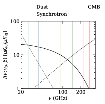
The two PySM models we consider are:
simset1 This corresponds to the ‘a1d1f1s1’ model of PySM, and the
‘standard’ model of SO19. It has power-law synchrotron emission with a
spatially varying synchrotron index estimated from WMAP data
Bennett et al. (2013). The dust emission
is described by a modified blackbody with ,
where is the temperature of the dust, and is the opacity index.
It has a spatially varying dust emissivity and temperature estimated from
Planck data. The emission of each component as a function of frequency is
shown in Fig 1.
simset2 This model modifies the synchrotron spectral index map of simset1 by adding power at small scales using a Gaussian realization of a power law power spectrum (Krachmalnicoff et al., 2018). This model is referred to as the ‘high-res ’ model used in SO19.
II.2 CMB
The PySM code simulates the primary CMB by creating Gaussian realizations of a given set of theoretical power spectra, calculated for a given cosmology. We use a theoretical power spectrum for the fiducial Planck 2018 cosmological parameters (Planck Collaboration, 2018), with no tensor-to-scalar ratio, . PySM uses the healpy implementation of synfast to generate primary CMB realizations of temperature and polarization. It then uses the taylens222https://github.com/amaurea/taylens (Naess and Louis, 2013) software to apply the displacements of the primary CMB caused by gravitational lensing.
| Frequency (GHz) | () | |||||
|---|---|---|---|---|---|---|
| optimistic | pessimistic | goal | baseline | |||
| 27 | 30 | 15 | -2.4 | 25 | 35 | 91 |
| 39 | 30 | 15 | -2.4 | 17 | 21 | 63 |
| 93 | 50 | 25 | -2.6 | 1.9 | 2.6 | 30 |
| 145 | 50 | 25 | -3.0 | 2.1 | 3.3 | 17 |
| 225 | 70 | 35 | -3.0 | 4.2 | 6.3 | 11 |
| 280 | 100 | 40 | -3.0 | 10 | 16 | 9 |
II.3 Sky area and expected noise levels
As described in SO19, the Simons Observatory plans to conduct two surveys: a large survey covering about 40% of the sky, conducted by the LAT, and a smaller survey of the cleanest of the sky using the SATs (Stevens et al., 2018).
The noise model used in this study is described in detail in SO19, and we summarize it here. Two noise levels are considered: the ‘baseline’ design assumes a raw sensitivity based on the achieved performance of previous ground based experiments such as ABS (Kusaka et al., 2018), BICEP (BICEP2 Collaboration and Keck Array Collaboration, 2016), and QUIET (QUIET Collaboration, 2011, 2012), and a ‘goal’ design which will require more abitious detector development. These raw sensitivities are multiplied by an observing efficiency of 20%, accounting for all data cuts, observing downtime and instrument calibration, based on the efficiency achieved during observations at the same site by the ACT experiment.
The noise induced in the insrument by atmospheric loading and instrument systematics is parameterized as an additional term in the noise power spectrum that increases at large scales:
| (3) |
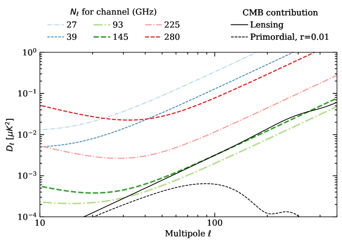
where and are the knee index and multipole, respectively. The range of parameters we consider here, as in SO19, are summarized in Table 1. In Figure 2 we show the individual frequency noise curves, from SO19, for the optimistic knee multipole, and goal sensitivity, compared to the lensing mode spectrum.
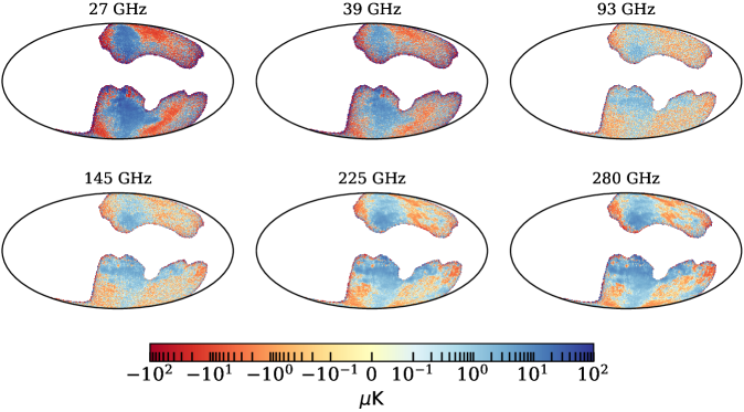
Due to the large field of view of the SAT, the survey design has non-uniform depth. Therefore, in modeling the noise properties it is important to weight noise realizations by the relative hit density. We follow the same procedure as in SO19 to generate noise realizations with this non-uniform hit density, and non-white noise.
In SO19, the effect of the resolution of the lowest two frequency channels on constraints on was studied. It was found that the impact of the resolution of these channels did not affect the achieved sensitivity dramatically. In order to simplify the later analysis, we therefore make the assumption that all frequencies have the same FWHM resolution.
We generate 200 Monte Carlo realizations of the noise and CMB, and use a common foreground realization for this suite of simulations.
III Component Separation and parameter estimation
In this section we describe the map-space component separation algorithm, and the subsequent estimation of power spectra and parameters from the cleaned maps.
III.1 Component separation
Our component separation method follows the BFoRe method described in Alonso et al. (2017). We take the simulated sky maps, , and model them as a linear combination of components with spatially varying SEDs, and noise:
| (4) |
where is the mixing matrix containing different component SEDs, with parameters , is a vector of component templates at a specific reference frequency, and is a noise term. Comparing to 2 we see that this is essentially the ‘correct’ model, modulo the permitted degree of spatial variation of the spectral parameters , and beam-convolution.
Under the assumption of Gaussian noise we can write down the likelihood for the data:
| (5) |
where is the data covariance. We simplify the analysis by assuming that the noise is diagonal in pixels and frequencies, however we emphasize that the true noise in non-white, making this approach sub-optimal. This assumption allows us to write the covariance as a diagonal matrix:
| (6) |
Under this assumption, the likelihood can be separated into a product over large pixels in which the spectral parameters are allowed to vary. In principle, these large pixels are not tied to any particular pixelization scheme, but can be implemented as any arbitrary shape intended to follow the true spatial variation of spectral parameters. The complexity of the foreground model can be increased by allowing more parameters to vary in the fit, or by increasing the number of independent patches.
Unless otherwise stated, during the rest of this paper we maximize the likelihood in equation 5 by varying only the dust and synchrotron spectral indices, and , keeping the temperature fixed at . We carry out this maximization in each large pixel, and for each Monte Carlo realization of CMB and noise. This is equivalent to marginalizing over the spectral indices for a single realization.
III.2 mode power spectrum estimation
In order to constrain the tensor-to-scalar ratio we first calculate the power spectrum from the cleaned CMB and maps. The transformation from to is inherently non local as it requires the calculation of spherical harmonic transforms:
| (7) |
where is a matrix, with each element being a specific combination of spin-weighted spherical harmonics (e.g., Grain et al., 2009).
Ground based instruments observe only part of the sky, and so can only access the true sky, multiplied by some window function, : . A naive calculation using the standard pseudo-power spectrum technique (Wandelt et al., 2001) will mix and modes, and if not accounted for increases the variance of the estimated modes, limiting the achievable constraints on the tensor-to-scalar ratio (Challinor and Chon, 2005; Smith, 2006).
To correct for this effect we use a ‘pure’ estimator of the power spectrum (Smith, 2006; Smith and Zaldarriaga, 2007; Grain et al., 2009), which is equivalent to first calculating the naive pseudo-spectrum of the maps over some mask, , and then calculating and removing the leaked modes (Grain et al., 2009). This method assumes that the applied mask satisfies Dirichlet and Neumann boundary conditions. Therefore, we apply an additional tapering to the inverse variance map that would usually be used in the calculation of the power spectrum. In this work we use the publicly available NaMaster333https://github.com/LSSTDESC/namaster code. For details of the implementation see the NaMaster documentation and Alonso et al. (2019), and for further theoretical background see Smith (2006); Smith and Zaldarriaga (2007); Grain et al. (2009).
Due to the limited sky coverage, there is insufficient information to invert the mode coupling matrix for all multipoles. Instead we coarse-grain the matrix by defining some binning scheme. In this work we use the binning operator:
| (8) |
where is the Heaviside function, denotes the bandpower, and is the width of each bin, which we choose to be . Then estimates of the binned power spectrum are:
| (9) |
From the cleaned Monte Carlo simulations we calculate the expected power spectrum, and its covariance. In order to avoid noise bias, we cross-correlate only cleaned maps with different noise realizations.
III.3 Cosmological parameter likelihood
The full posterior for the individual bandpowers is non-Gaussian. However, for high enough multipoles the central limit theorem justifies a Gaussian approximation Hamimeche and Lewis (2008). The combination of the compact observing region and atmosphere-induced systematics, limit constraints on large scale modes. Therefore, we consider only , for which the Gaussian approximation is valid:
| (10) | ||||
where the measured power spectrum is indicated by the hat, and the model, , is the sum of a primordial term and a lensing term, is a template for the lensing contribution, and is a template for the primordial contribution, both of which are calculated using the CLASS code with Planck 2018 cosmological parameters (Planck Collaboration, 2018) and . Equations 10 are given at the bandpowers , having accounted for the effects of bandpower averaging and inversion of the mode coupling matrix (e.g., Grain et al., 2009; Alonso et al., 2019).
We sample this likelihood for these two parameters using the emcee package, and summarize the posterior on by marginalizing over the lensing amplitude and calculating the median and standard deviation of the posterior distribution.
IV Results
In this section we present the results of applying the foreground separation algorithm described in Section III to the simulations described in Section II.
We first present the results for simset1, which are the fiducial sky simulations analyzed in SO19. As noted, the foreground-cleaning algorithm presented in this paper is similar to the BFoRe method used in The Simons Observatory Collaboration (2019) and Alonso et al. (2017), but uses an independent pipeline. Therefore, we first validate our analysis, and then provide an extension of the cases studied in previous works.
IV.1 Fiducial sky simulations
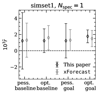
We show the resulting bias and uncertainty on for the four Simons Observatory noise configurations in Figure 4, compared to the results of the xForecast (Errard and Stompor, 2019) framework presented in SO19. We compare to xForecast, an alternative parametric method that uses the same simulations, because the reported BFoRe forecasts in SO19 include an additional marginalization over residual foregrounds while estimating the tensor-to-scalar ratio. This comparison is therefore done for the specific xForecast case where no additional foreground power is marginalized over. Figure 4 shows that our method produces consistent forecasts with those in SO19. The nominal Simons Observatory design is biased by 1, and the most sensitive design is biased by 2. The errors from our method and xForecast are not identical; we have checked (private communication) that our forecasted errors agree with the BFoRe code in the case of no-marginalization.
In the rest of this section we focus on the case of optimistic and baseline sensitivity. We demonstrate that the source of the bias in is due to foreground contamination, primarily from residual dust. In SO19 the bias was largely removed at the power spectrum level by marginalizing over a template power spectrum for the foreground contamination. Relying on this method for an unbiased detection of primordial gravitational waves could be problematic as the shape of the residual foreground power spectrum is not known a priori.
In the rest of this section we establish that neglecting spatial variation of the indices is the root cause of the bias, and that it may be removed with additional masking of the higher-foreground regions, or by introducing only a few more parameters describing the spatial variation of the dust spectral parameters.
IV.2 Establishing source of bias
IV.2.1 Masking the Galactic plane
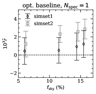
To establish the root of a non-zero value of , the result must be robust against different splits of the data. In this section we establish that increasing the masking of the Galactic plane when estimating the power spectrum from cleaned CMB maps reduces the spurious detection of , and we show that sufficient masking can remove all of the bias in , at the expense of a small increase in the uncertainty.
We use a set of Galactic masks based on thresholds of the Planck intensity maps at 353 GHz, downloaded from the Planck Legacy Archive 444 Filename: HFI_Mask_GalPlane-apo0_2048_R2.00.fits. The masks range from leaving 20 % to 80 % of the sky unmasked. We combine each Planck mask with the SO hits map from SO19, resulting in four maps with effective sky area from % to , calculated using the appropriate expression for noise-dominated maps (The Simons Observatory Collaboration, 2019):
| (11) |
where is the combined hit map, and Galactic mask. For each mask we repeat the power spectrum estimation and cosmological parameter fitting to estimate , and present the results in Figure 6. As the masks become more aggressive, the bias in is reduced substantially for both simset1 and simset2. Since we expect foreground residuals to be localized to the Galactic plane, a decreasing bias with increased plane masking indicates the Galactic nature of the bias.
IV.2.2 Cross-correlating with foreground templates
If the cleaned CMB maps are contaminated by foreground residuals, we may expect there to be a significant correlation with templates of the individual foreground components. In order to perform this test using only the observed data, without relying on external observations, we form templates of high and low frequency foregrounds in the following way.
A synchrotron template is constructed by differencing the 27 GHz and 40 GHz maps, and a dust template is constructed by differencing the 270 GHz and 220 GHz maps. In thermodynamic units the CMB contribution will cancel, and we will be left with a map proportional to the synchrotron and dust populations, respectively. The foreground templates are then correlated with the cleaned CMB maps. We may expect the noise in the constructed templates and cleaned CMB maps to be correlated, leading to biases in the recovered power spectra. Therefore, we only correlate templates and CMB maps from different half-mission splits of the data. Recent work (e.g., Clark et al., 2015; Clark, 2018) has shown that linear Galactic neutral hydrogen features are correlated with polarized Galactic foregrounds. Maps of HI emission could provide an independent test of polarized dust contamination in cleaned CMB maps.
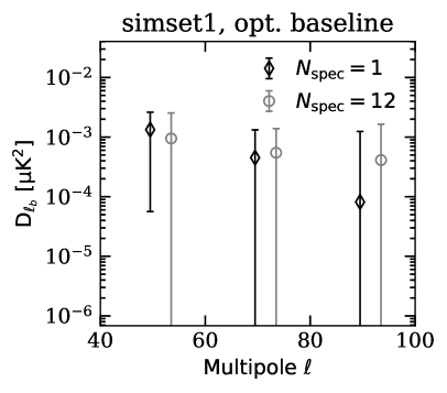
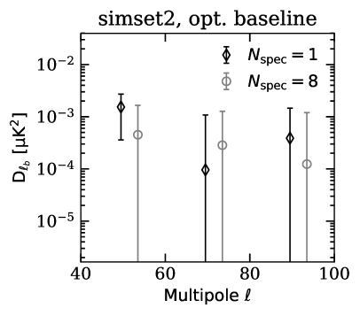
In Figure 5 we show the cross spectra of simset1 and simset2 with dust and synchrotron templates, respectively, using the largest 16% sky region and cleaning with a single synchrotron and dust index. We find that the residual foregrounds, which showed up as a bias in in Figure 4, can be detected in the cross-spectra.
From these exercises we find that: i) a single spectral parameter is insufficient to describe the spectral energy dependence of foregrounds in the region observed by the Simons Observatory, and results in a bias for the most optimistic case of foreground complexity, as was found in SO19. ii) depending on the complexity of the true foregrounds, the bias can be primarily due to dust or to synchrotron contamination, iii) the bias can be mostly removed by using only 6 % of the sky. These conclusions are true in so far as these simulations are representative of the true sky, which may in fact be more complicated.
IV.3 Spatially varying spectral indices
In this sub-section we demonstrate that the residual foreground contamination occurs because the fitting process does not account for the spatial variation of the spectral indices, and we demonstrate that such variation may be sufficiently described by only a few additional parameters if they could be chosen to accurately capture the spatial variation.
We adapt the map-space cleaning algorithm to account for spatial variation of the foregrounds by defining a set of patches in which to fit spectral indices. In theory , where corresponds to fitting a single spectral index over the whole sky, and fits a spectral index in every pixel at the resolution of the input maps. The limit of large would account for as much spatial variation in the foreground SEDs as possible, however requires increasing the number of fitted parameters, and therefore post-separation noise. It would therefore be ideal to keep as low as possible, whilst still achieving an unbiased estimation of . These simulations were generated at resolution, therefore, there would be no advantage to choosing . Note that, for observations of the real sky, the creation of pixelized maps requires spatial averaging both along the line of sight, and transverse to it. Such averaging could be better fitted by taking , as the extra parameters could absorb some of the resulting SED curvature (Chluba et al., 2017; Krachmalnicoff et al., 2018). Recent work (such as the moment-based expansion of Chluba et al., 2017) has suggested introducing additional parameters in the SED to capture the effects of spectral variations at smaller scales. This would avoid the complication of deciding how to subdivide the sky. Comparison to this approach would be interesting, and is left for future work.
How to distribute patches on the sky is an important consideration, as it involves a choice of how to model the spatial dependence of foreground parameters. This is unknown a priori, so we explore an initial exploration of possible approaches.

IV.3.1 Fitting spectral indices on a HEALPix grid
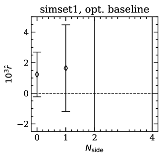
Some previous studies have used patches corresponding to a coarse HEALPix grid for convenience (e.g., Alonso et al., 2017), allowing an independent spectral parameter to be fit in each coarse pixel, as shown in the right panel of Figure 7. We define a set of fitting models with spectral parameters varying on grids at (with ), and perform the foreground cleaning. We show our resulting constraints on in Figure 8. We find that the errors are significantly inflated as increases, but determine that this is partly due to many of the larger Healpix pixels having too few observed pixels, and also due to having so many additional parameters.
IV.3.2 With prior information on spatial variation of indices
With prior information about the spatial variation of the spectral parameters we investigate how many additional parameters would be needed to mitigate the observed biases in due to foreground residuals. Here we use the dust spectral index map, , used in PySM model ‘d1’, to create a template that defines the regions in which we fit spectral parameters. The method used to define regions from is described in detail in Algorithm 1.
We repeat Algorithm 1 for , to produce twelve different template maps, with increasing spatial resolution. Figure 7 shows the regions for .
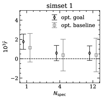
We run our foreground cleaning algorithm on the simset1 sky simulations for these spectral index pixelizations described above. The resulting constraints we find on are shown in Figure 9 for . We find that increasing results in a reduced bias on , as we are able to account for spatial variation of , with negligible inflation of the uncertainty. No improvement of the bias is achieved past a value of . Since the fitting code is designed to fit all parameters in the same patches, this remaining bias is due to the mismatch between the dust-focused fitting regions and synchrotron spectral index variation. Modifying the fitting code to allow different physical parameters to be fitted with different constraints is a non-trivial extension, and is left to future work.
In Figure 5 we show the cross-correlation of the cleaned CMB maps with the dust foreground templates, as a function of number of fitting pixels . Increasing the number of fitting regions results in a better cleaning of the foregrounds, and consequently we find no signature of residual contamination by .
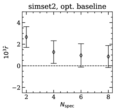
We then repeat this study for simset2, which has a synchrotron spectral index with a greater spatial variance, . Ignoring spatial variation of the foreground SED in this case results in an even larger bias on than in the case of simset1. Here we use to define the sky regions used for fitting the indices, and as the input for Algorithm 1. Our resulting constraints on are shown in Figure 9. Again, there is a reduction in the bias on as we increase , and the improvement saturates at . For we see no improvement as the bias is now dominated by residuals due to dust mis-modeling. Indeed the remaining bias for is at the level found when fitting simset1 with a single spectral index.
In Figure 5 we show the correlation of the cleaned CMB maps with a synchrotron template formed from the two lowest frequency channels. Similar to simset1 we find that increasing removes the hints of foreground bias at low multipoles seen when ignoring spatial variation of spectral indices.
It is promising that with only 4-6 additional parameters describing the spatial variation of the synchrotron and dust indices, that a 1-3 bias in might be mitigated without significant masking. In practice, though, we will not have the perfect information about their spatial variation. There may also be additional variation not captured in the existing simulations. Instead, we would need to derive the fitting regions directly from the data.
Towards this, we determined that the of the model compared to the data, with the intent to add spatial resolution to the fitting model in areas of poor , was not sufficiently sensitive to discriminate between areas of good and poor fit. A judicious choice of these fitting regions, based on existing and upcoming observations, will be a natural direction for future study.
V Conclusions
By accounting for Galactic foreground models based on current data, we have assessed how large-scale mode observations of the Simons Observatory might be used to constrain the tensor-to-scalar ratio, following on from the forecast study in SO19. We showed that the nominal SO design may result in a biased estimation of due to foreground contamination, which can either be mitigated by marginalizing over a foreground residual after cleaning the maps, or by restricting the sky area to discard the most contaminated region. This masking removes or reduces this bias to one standard deviation or less.
In a further alternative approach, we defined a scheme to allow for spatial variation in the parameterization of the fitted foreground model. We found that using Healpix pixels was unsatisfactory, as the coarse-grained pixels that overlapped the observed regions were not fitted reliably, and could lead to large residuals. We also defined a new spatial parameterization that split the sky into an arbitrary number of regions following the true morphology of the spectral behavior of the dominant foreground contaminant. With this approach, with perfect knowledge of the spectral index variation, we found that fitting 4-6 independent regions was sufficient to remove the dominant -bias. This points to a direction for further exploration in choosing the regions from the real data. We found that the cross-correlation of the cleaned maps with the tracers of synchrotron and dust provide a useful way to check for residual foregrounds that bias the estimate for . In practice, a comprehensive analysis of the real data from SO will likely implement a set of these bias-mitigation approaches, coupled with alternative non-parametric methods for foreground cleaning, internal null tests to check for consistency, and tests for residual non-Gaussianity of the maps.
Acknowledgements.
We acknowledge the use of Healpix. BT acknowledges the support of an STFC studentship. DA acknowledges support from STFC through an Ernest Rutherford Fellowship, grant reference ST/P004474/1. MA acknowledges the support from the Beecroft Trust. JE acknowledges support of the French National Research Agency (Agence National de Recherche) grant, ANR BB 555www.bxb.space. This is not an official Simons Observatory Collaboration paper.References
- The Simons Observatory Collaboration (2019) The Simons Observatory Collaboration, Journal of Cosmology and Astro-Particle Physics 2019, 056 (2019), arXiv:1808.07445 [astro-ph.CO] .
- Hui et al. (2018) H. Hui, P. A. R. Ade, Z. Ahmed, R. W. Aikin, K. D. Alexander, D. Barkats, S. J. Benton, C. A. Bischoff, J. J. Bock, R. Bowens-Rubin, J. A. Brevik, I. Buder, E. Bullock, V. Buza, J. Connors, J. Cornelison, B. P. Crill, M. Crumrine, M. Dierickx, L. Duband, C. Dvorkin, J. P. Filippini, S. Fliescher, J. Grayson, G. Hall, M. Halpern, S. Harrison, S. R. Hildebrand t, G. C. Hilton, K. D. Irwin, J. Kang, K. S. Karkare, E. Karpel, J. P. Kaufman, B. G. Keating, S. Kefeli, S. A. Kernasovskiy, J. M. Kovac, C. L. Kuo, K. Lau, N. A. Larsen, E. M. Leitch, M. Lueker, K. G. Megerian, L. Moncelsi, T. Namikawa, C. B. Netterfield, H. T. Nguyen, R. O’Brient, R. W. Ogburn, S. Palladino, C. Pryke, B. Racine, S. Richter, R. Schwarz, A. Schillaci, C. D. Sheehy, A. Soliman, T. St. Germaine, Z. K. Staniszewski, B. Steinbach, R. V. Sudiwala, G. P. Teply, K. L. Thompson, J. E. Tolan, C. Tucker, A. D. Turner, C. Umiltà, A. G. Vieregg, A. Wand ui, A. C. Weber, D. V. Wiebe, J. Willmert, C. L. Wong, W. L. K. Wu, E. Yang, K. W. Yoon, and C. Zhang, in Millimeter, Submillimeter, and Far-Infrared Detectors and Instrumentation for Astronomy IX, Society of Photo-Optical Instrumentation Engineers (SPIE) Conference Series, Vol. 10708 (2018) p. 1070807, arXiv:1808.00568 [astro-ph.IM] .
- Planck Collaboration (2018) Planck Collaboration, arXiv e-prints , arXiv:1807.06209 (2018), arXiv:1807.06209 [astro-ph.CO] .
- Kamionkowski et al. (1997) M. Kamionkowski, A. Kosowsky, and A. Stebbins, Phys. Rev. D 55, 7368 (1997).
- Seljak and Zaldarriaga (1996) U. Seljak and M. Zaldarriaga, Astrophys. J. 469, 437 (1996), arXiv:astro-ph/9603033 [astro-ph] .
- Ijjas and Steinhardt (2018) A. Ijjas and P. J. Steinhardt, Classical and Quantum Gravity 35, 135004 (2018), arXiv:1803.01961 .
- BICEP2 Collaboration and Keck Array Collaboration (2018) BICEP2 Collaboration and Keck Array Collaboration, Physical Review Letters 121, 221301 (2018), arXiv:1810.05216 .
- Thornton et al. (2016) R. J. Thornton, P. A. R. Ade, S. Aiola, F. E. Angilè, M. Amiri, J. A. Beall, D. T. Becker, H.-M. Cho, S. K. Choi, P. Corlies, K. P. Coughlin, R. Datta, M. J. Devlin, S. R. Dicker, R. Dünner, J. W. Fowler, A. E. Fox, P. A. Gallardo, J. Gao, E. Grace, M. Halpern, M. Hasselfield, S. W. Henderson, G. C. Hilton, A. D. Hincks, S. P. Ho, J. Hubmayr, K. D. Irwin, J. Klein, B. Koopman, D. Li, T. Louis, M. Lungu, L. Maurin, J. McMahon, C. D. Munson, S. Naess, F. Nati, L. Newburgh, J. Nibarger, M. D. Niemack, P. Niraula, M. R. Nolta, L. A. Page, C. G. Pappas, A. Schillaci, B. L. Schmitt, N. Sehgal, J. L. Sievers, S. M. Simon, S. T. Staggs, C. Tucker, M. Uehara, J. van Lanen, J. T. Ward, and E. J. Wollack, ApJ 227, 21 (2016), arXiv:1605.06569 [astro-ph.IM] .
- Benson et al. (2014) B. A. Benson, P. A. R. Ade, Z. Ahmed, S. W. Allen, K. Arnold, J. E. Austermann, A. N. Bender, L. E. Bleem, J. E. Carlstrom, C. L. Chang, H. M. Cho, J. F. Cliche, T. M. Crawford, A. Cukierman, T. de Haan, M. A. Dobbs, D. Dutcher, W. Everett, A. Gilbert, N. W. Halverson, D. Hanson, N. L. Harrington, K. Hattori, J. W. Henning, G. C. Hilton, G. P. Holder, W. L. Holzapfel, K. D. Irwin, R. Keisler, L. Knox, D. Kubik, C. L. Kuo, A. T. Lee, E. M. Leitch, D. Li, M. McDonald, S. S. Meyer, J. Montgomery, M. Myers, T. Natoli, H. Nguyen, V. Novosad, S. Padin, Z. Pan, J. Pearson, C. Reichardt, J. E. Ruhl, B. R. Saliwanchik, G. Simard, G. Smecher, J. T. Sayre, E. Shirokoff, A. A. Stark, K. Story, A. Suzuki, K. L. Thompson, C. Tucker, K. Vanderlinde, J. D. Vieira, A. Vikhlinin, G. Wang, V. Yefremenko, and K. W. Yoon, in Millimeter, Submillimeter, and Far-Infrared Detectors and Instrumentation for Astronomy VII, PROCSPIE, Vol. 9153 (2014) p. 91531P, arXiv:1407.2973 [astro-ph.IM] .
- Kang et al. (2018) J. H. Kang, P. A. R. Ade, Z. Ahmed, R. W. Aikin, K. D. Alexander, D. Barkats, S. J. Benton, C. A. Bischoff, J. J. Bock, H. Boenish, R. Bowens-Rubin, J. A. Brevik, I. Buder, E. Bullock, V. Buza, J. Connors, J. Cornelison, B. P. Crill, M. Crumrine, M. Dierickx, L. Duband, C. Dvorkin, J. P. Filippini, S. Fliescher, J. A. Grayson, G. Hall, M. Halpern, S. Harrison, S. R. Hildebrandt, G. C. Hilton, H. Hui, K. D. Irwin, K. S. Karkare, E. Karpel, J. P. Kaufman, B. G. Keating, S. Kefeli, S. A. Kernasovskiy, J. M. Kovac, C. L. Kuo, N. A. Larsen, K. Lau, E. M. Leitch, M. Lueker, K. G. Megerian, L. Moncelsi, T. Namikawa, B. Netterfield, H. T. Nguyen, R. O’Brient, R. W. Ogburn, S. Palladino, C. Pryke, B. Racine, S. Richter, A. Schillaci, R. Schwarz, C. D. Sheehy, A. Soliman, T. St. Germaine, Z. K. Staniszewski, B. Steinbach, R. V. Sudiwala, G. P. Teply, K. L. Thompson, J. E. Tolan, C. Tucker, A. D. Turner, C. Umiltà, A. G. Vieregg, A. Wandui, A. C. Weber, D. V. Wiebe, J. Willmert, C. L. Wong, W. L. K. Wu, H. Yang, W. Yoon, K., and C. Zhang, in Millimeter, Submillimeter, and Far-Infrared Detectors and Instrumentation for Astronomy IX, Society of Photo-Optical Instrumentation Engineers (SPIE) Conference Series, Vol. 10708 (2018) p. 107082N, arXiv:1808.00567 [astro-ph.IM] .
- Suzuki et al. (2016) A. Suzuki, P. Ade, Y. Akiba, C. Aleman, K. Arnold, C. Baccigalupi, B. Barch, D. Barron, A. Bender, D. Boettger, J. Borrill, S. Chapman, Y. Chinone, A. Cukierman, M. Dobbs, A. Ducout, R. Dunner, T. Elleflot, J. Errard, G. Fabbian, S. Feeney, C. Feng, T. Fujino, G. Fuller, A. Gilbert, N. Goeckner-Wald, J. Groh, T. D. Haan, G. Hall, N. Halverson, T. Hamada, M. Hasegawa, K. Hattori, M. Hazumi, C. Hill, W. Holzapfel, Y. Hori, L. Howe, Y. Inoue, F. Irie, G. Jaehnig, A. Jaffe, O. Jeong, N. Katayama, J. Kaufman, K. Kazemzadeh, B. Keating, Z. Kermish, R. Keskitalo, T. Kisner, A. Kusaka, M. L. Jeune, A. Lee, D. Leon, E. Linder, L. Lowry, F. Matsuda, T. Matsumura, N. Miller, K. Mizukami, J. Montgomery, M. Navaroli, H. Nishino, J. Peloton, D. Poletti, G. Puglisi, G. Rebeiz, C. Raum, C. Reichardt, P. Richards, C. Ross, K. Rotermund, Y. Segawa, B. Sherwin, I. Shirley, P. Siritanasak, N. Stebor, R. Stompor, J. Suzuki, O. Tajima, S. Takada, S. Takakura, S. Takatori, A. Tikhomirov, T. Tomaru, B. Westbrook, N. Whitehorn, T. Yamashita, A. Zahn, and O. Zahn, Journal of Low Temperature Physics 184, 805 (2016), arXiv:1512.07299 [astro-ph.IM] .
- Chuss et al. (2016) D. T. Chuss, A. Ali, M. Amiri, J. Appel, C. L. Bennett, F. Colazo, K. L. Denis, R. Dünner, T. Essinger-Hileman, J. Eimer, P. Fluxa, D. Gothe, M. Halpern, K. Harrington, G. Hilton, G. Hinshaw, J. Hubmayr, J. Iuliano, T. A. Marriage, N. Miller, S. H. Moseley, G. Mumby, M. Petroff, C. Reintsema, K. Rostem, K. U-Yen, D. Watts, E. Wagner, E. J. Wollack, Z. Xu, and L. Zeng, Journal of Low Temperature Physics 184, 759 (2016), arXiv:1511.04414 [astro-ph.IM] .
- Krachmalnicoff et al. (2018) N. Krachmalnicoff, E. Carretti, C. Baccigalupi, G. Bernardi, S. Brown, B. M. Gaensler, M. Haverkorn, M. Kesteven, F. Perrotta, S. Poppi, and L. Staveley-Smith, ArXiv e-prints (2018), arXiv:1802.01145 .
- Lewis and Challinor (2006) A. Lewis and A. Challinor, PhysRep 429, 1 (2006), astro-ph/0601594 .
- Eriksen et al. (2008) H. K. Eriksen, J. B. Jewell, C. Dickinson, A. J. Banday, K. M. Górski, and C. R. Lawrence, Astrophys. J. 676, 10 (2008), arXiv:0709.1058 .
- Alonso et al. (2017) D. Alonso, J. Dunkley, B. Thorne, and S. Næss, Physical Review D 95, 043504 (2017).
- Remazeilles et al. (2018) M. Remazeilles, A. J. Banday, C. Baccigalupi, S. Basak, A. Bonaldi, G. De Zotti, J. Delabrouille, C. Dickinson, H. K. Eriksen, J. Errard, R. Fernandez-Cobos, U. Fuskeland, C. Hervías-Caimapo, M. López-Caniego, E. Martinez-González, M. Roman, P. Vielva, I. Wehus, A. Achucarro, P. Ade, R. Allison, M. Ashdown, M. Ballardini, R. Banerji, J. Bartlett, N. Bartolo, D. Baumann, M. Bersanelli, M. Bonato, J. Borrill, F. Bouchet, F. Boulanger, T. Brinckmann, M. Bucher, C. Burigana, A. Buzzelli, Z.-Y. Cai, M. Calvo, C.-S. Carvalho, G. Castellano, A. Challinor, J. Chluba, S. Clesse, I. Colantoni, A. Coppolecchia, M. Crook, G. D’Alessandro, P. de Bernardis, G. de Gasperis, J.-M. Diego, E. Di Valentino, S. Feeney, S. Ferraro, F. Finelli, F. Forastieri, S. Galli, R. Genova-Santos, M. Gerbino, J. González-Nuevo, S. Grandis, J. Greenslade, S. Hagstotz, S. Hanany, W. Handley, C. Hernandez-Monteagudo, M. Hills, E. Hivon, K. Kiiveri, T. Kisner, T. Kitching, M. Kunz, H. Kurki-Suonio, L. Lamagna, A. Lasenby, M. Lattanzi, J. Lesgourgues, A. Lewis, M. Liguori, V. Lindholm, G. Luzzi, B. Maffei, C. J. A. P. Martins, S. Masi, S. Matarrese, D. McCarthy, J.-B. Melin, A. Melchiorri, D. Molinari, A. Monfardini, P. Natoli, M. Negrello, A. Notari, A. Paiella, D. Paoletti, G. Patanchon, M. Piat, G. Pisano, L. Polastri, G. Polenta, A. Pollo, V. Poulin, M. Quartin, J.-A. Rubino-Martin, L. Salvati, A. Tartari, M. Tomasi, D. Tramonte, N. Trappe, T. Trombetti, C. Tucker, J. Valiviita, R. Van de Weijgaert, B. van Tent, V. Vennin, N. Vittorio, K. Young, and M. Zannoni, JCAP 4, 023 (2018), arXiv:1704.04501 .
- Note (1) https://github.com/bthorne93/PySM_public.
- Thorne et al. (2017) B. Thorne, J. Dunkley, D. Alonso, and S. Næss, Monthly Notices of the Royal Astronomical Society 469, 2821 (2017).
- Bennett et al. (2013) C. L. Bennett, D. Larson, J. L. Weiland, N. Jarosik, G. Hinshaw, N. Odegard, K. M. Smith, R. S. Hill, B. Gold, M. Halpern, E. Komatsu, M. R. Nolta, L. Page, D. N. Spergel, E. Wollack, J. Dunkley, A. Kogut, M. Limon, S. S. Meyer, G. S. Tucker, and E. L. Wright, The Astrophysical Journal Supplement Series 208, 20 (2013).
- Note (2) https://github.com/amaurea/taylens.
- Naess and Louis (2013) S. K. Naess and T. Louis, JCAP 9, 001 (2013), arXiv:1307.0719 .
- Stevens et al. (2018) J. R. Stevens, N. Goeckner-Wald, R. Keskitalo, N. McCallum, A. Ali, J. Borrill, M. L. Brown, Y. Chinone, P. A. Gallardo, A. Kusaka, A. T. Lee, J. McMahon, M. D. Niemack, L. Page, G. Puglisi, M. Salatino, S. Y. D. Mak, G. Teply, D. B. Thomas, E. M. Vavagiakis, E. J. Wollack, Z. Xu, and N. Zhu, in Millimeter, Submillimeter, and Far-Infrared Detectors and Instrumentation for Astronomy IX, Society of Photo-Optical Instrumentation Engineers (SPIE) Conference Series, Vol. 10708 (2018) p. 1070841, arXiv:1808.05131 [astro-ph.IM] .
- Kusaka et al. (2018) A. Kusaka, J. Appel, T. Essinger-Hileman, J. A. Beall, L. E. Campusano, H.-M. Cho, S. K. Choi, K. Crowley, J. W. Fowler, P. Gallardo, M. Hasselfield, G. Hilton, S.-P. P. Ho, K. Irwin, N. Jarosik, M. D. Niemack, G. W. Nixon, M. Nolta, J. Page, Lyman A., G. A. Palma, L. Parker, S. Raghunathan, C. D. Reintsema, J. Sievers, S. M. Simon, S. T. Staggs, K. Visnjic, and K.-W. Yoon, Journal of Cosmology and Astro-Particle Physics 2018, 005 (2018), arXiv:1801.01218 [astro-ph.CO] .
- BICEP2 Collaboration and Keck Array Collaboration (2016) BICEP2 Collaboration and Keck Array Collaboration, Phys. Rev. Lett. 116, 031302 (2016), arXiv:1510.09217 [astro-ph.CO] .
- QUIET Collaboration (2011) QUIET Collaboration, Astrophys. J. 741, 111 (2011), arXiv:1012.3191 [astro-ph.CO] .
- QUIET Collaboration (2012) QUIET Collaboration, Astrophys. J. 760, 145 (2012), arXiv:1207.5034 [astro-ph.CO] .
- Grain et al. (2009) J. Grain, M. Tristram, and R. Stompor, Physical Review D 79, 123515 (2009), arXiv:0903.2350 [astro-ph.CO] .
- Wandelt et al. (2001) B. D. Wandelt, E. Hivon, and K. M. Górski, Phys. Rev. D 64, 083003 (2001).
- Challinor and Chon (2005) A. Challinor and G. Chon, MNRAS 360, 509 (2005), astro-ph/0410097 .
- Smith (2006) K. M. Smith, Phys. Rev. D 74, 083002 (2006), astro-ph/0511629 .
- Smith and Zaldarriaga (2007) K. M. Smith and M. Zaldarriaga, Phys. Rev. D 76, 043001 (2007), astro-ph/0610059 .
- Note (3) https://github.com/LSSTDESC/namaster.
- Alonso et al. (2019) D. Alonso, J. Sanchez, and A. Slosar, MNRAS 484, 4127 (2019), arXiv:1809.09603 [astro-ph.CO] .
- Hamimeche and Lewis (2008) S. Hamimeche and A. Lewis, Phys. Rev. D 77, 103013 (2008), arXiv:0801.0554 [astro-ph] .
- Errard and Stompor (2019) J. Errard and R. Stompor, Phys. Rev. D 99, 043529 (2019), arXiv:1811.00479 [astro-ph.CO] .
- Note (4) Filename: HFI_Mask_GalPlane-apo0_2048_R2.00.fits.
- Clark et al. (2015) S. E. Clark, J. C. Hill, J. E. G. Peek, M. E. Putman, and B. L. Babler, Phys. Rev. Lett. 115, 241302 (2015), arXiv:1508.07005 [astro-ph.CO] .
- Clark (2018) S. E. Clark, Astrophys. J. 857, L10 (2018), arXiv:1802.00011 [astro-ph.GA] .
- Chluba et al. (2017) J. Chluba, J. C. Hill, and M. H. Abitbol, MNRAS 472, 1195 (2017), arXiv:1701.00274 [astro-ph.CO] .
- Note (5) www.bxb.space.