Evolving neural networks to follow trajectories of arbitrary complexity

Abstract

Many experiments have been performed that use evolutionary algorithms for learning the topology and connection weights of a neural network that controls a robot or virtual agent. These experiments are not only performed to better understand basic biological principles, but also with the hope that with further progress of the methods, they will become competitive for automatically creating robot behaviors of interest. However, current methods are limited with respect to the (Kolmogorov) complexity of evolved behavior. Using the evolution of robot trajectories as an example, we show that by adding four features, namely (1) freezing of previously evolved structure, (2) temporal scaffolding, (3) a homogeneous transfer function for output nodes, and (4) mutations that create new pathways to outputs, to standard methods for the evolution of neural networks, we can achieve an approximately linear growth of the complexity of behavior over thousands of generations. Overall, evolved complexity is up to two orders of magnitude over that achieved by standard methods in the experiments reported here, with the major limiting factor for further growth being the available run time. Thus, the set of methods proposed here promises to be a useful addition to various current neuroevolution methods.

This is the authors’ version of the accepted manuscript, the final and definite version can be found at https://doi.org/10.1016/j.neunet.2019.04.013. This version is available subject to a Creative Commons 4.0 CC-BY-NC-ND license.

¹Department of Computing and Technology, Nottingham Trent University, United Kingdom

²Max Planck Institute for Mathematics in the Sciences, Leipzig Germany

³Santa Fe Institute, Santa Fe, New Mexico, USA

1 Introduction

Evolutionary algorithms have been used successfully to solve various optimization problems including for scheduling, symbolic regression in astronomy, optimizing antenna designs and shapes of car parts, finding electronic circuits that perform a given function, and game playing (Poli et al.,, 2008; Eiben and Smith,, 2015). Similarly, neural networks have many important applications, including recognition of speech and handwritten digits, and robot control (Schmidhuber,, 2015). Topologies and connection weights of neural networks can be optimized by evolutionary algorithms (Floreano et al.,, 2008), and the resulting networks can be used to control robots, as has been done for some decades in the field of evolutionary robotics (Nolfi and Floreano,, 2000). Nevertheless, there are still very few real world applications of evolutionary robotics, and progress towards more complex behaviors of interest seems to be slow (Doncieux et al.,, 2015; Pugh et al.,, 2016).

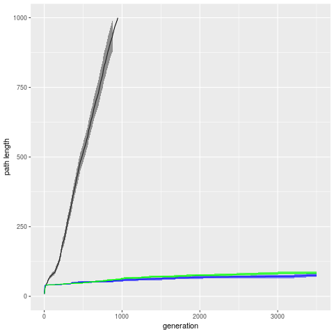
For many of the earliest evolutionary robotics experiments, neural networks with a fixed topology, i.e., a fixed number of nodes and connections, were used (Nolfi and Floreano,, 2000). That way, the achievable complexity of behavior is obviously limited. Later, methods were introduced that could increase these numbers. Perhaps the most well known of these is the method called NEAT (Stanley and Miikkulainen,, 2002). This neuroevolution method starts evolution using networks without any hidden nodes and subsequently adds neurons and connections by carefully designed mutation operators. It has been shown that complexification during evolution does indeed occur when using NEAT, and can create neural networks with in the order of up to a few dozens of neurons (Stanley and Miikkulainen,, 2004). NEAT has subsequently been widely used for various evolutionary robotics experiments. A more recent achievement is the development of methods that can produce large neural networks from comparatively small genomes. Some methods such as HyperNEAT (Stanley et al.,, 2009) and Compressed Network Complexity Search (Koutník et al.,, 2010; Gomez et al.,, 2012) achieve this by evolving a process that constructs the neural network instead of evolving the neural network directly. Other methods still evolve parts of the network directly, but make use of user-specified constraints (e.g., ICONE, Rempis and Pasemann, (2012)) or design patterns with evolvable parameters (e.g., NEATfields, Inden et al., (2012)) to create larger networks from those parts. While evolution can produce comparatively complex networks with hundreds of neurons using these methods, the complexity of the behavior that can be produced by evolution (as opposed to behavior that emerges from the coupling to a complex environment) is still limited, with the increase of both complexity and fitness typically converging towards zero after several hundred or thousand generations.

We have previously argued (Inden and Jost,, 2013) that this is unavoidable with the way artificial evolution is typically set up: A genome of fixed length can only produce a limited number of behaviors (and therefore there is an upper bound to complexity). A growing genome, on the other hand, cannot grow indefinitely because either mutations will overpower selection (in the case of fixed per-gene mutation rates, as discovered by Eigen, (1971)) or the waiting times for mutations on individual genes grow without bound (in the case of fixed per-genome mutation rates). However, evolution can in principle get around this problem by changing the genetic architecture such that mutations will with a higher than uniform probability occur where they are needed. It has actually been found that different regions in animal genomes are subject to different mutation rates, and that this is under genetic control (Martincorena et al.,, 2012). Evolution would be optimally adaptive if previously evolved useful features of an organism were conserved by a reduction of the local mutation rates, whereas features under adaptive evolution had increased local mutation rates. The starting point for this paper is a previously proposed method to guide mutations towards features under active evolution, and away from previously evolved adaptive features (Inden and Jost,, 2013). The basic idea is that only those parts of a neural network that were created by mutations most recently can be mutated. Older structures are frozen and cannot be mutated any more.

The idea of freezing evolved structure is not new, but has been explored a number of times, typically in connection with modular neural networks (Hülse et al.,, 2004; Togelius,, 2004). Incrementality has also been a part of traditional neural network architectures trained by supervised learning such as Cascade-Correlation networks (Fahlman and Lebiere,, 1990). It has also played a key role within the evolving spiking neural network models that were developed within a framework termed evolving connectionist systems. In those models, the learning procedure typically adds new neurons for new items of data to be learned without affecting existing neurons much. The neural networks considered in that framework are feed-forward networks (in some cases with additional structures such as evolving feature selectors, or dynamic reservoirs) used for classification tasks (Schliebs and Kasabov,, 2013). Recently, approaches that use evolution to learn a suitable architecture for a deep neural network (typically a convolutional neural network) that is trained by supervised methods have also become quite popular (Real et al.,, 2017; Miikkulainen et al.,, 2019; Liu et al.,, 2018). This research has shown that evolved architectures can solve difficult pattern recognition tasks with many inputs, classes, and samples, and are often superior in that regard to hand-designed architectures. However, as the architecture grows in size during evolution, two effects can be expected: For one, the same convergence as described above because the genome size increases. In addition, variance will increase for the supervised learning tasks, which in turn increases the time required for training the weights (Geman et al.,, 1992). Convolutional neural networks use techniques such as weight sharing to mitigate the latter problem. Recently, freezing of structure has also been explored within this context. Rusu et al., (2016) train columns of a deep neural network on different tasks one by one. The connection weights in earlier evolved columns are frozen, but lateral connections to newer columns are trained to allow for transfer of skills between different tasks. Similarly, Terekhov et al., (2015) train a series of blocks of neural networks on a series of related tasks, where the weights in earlier blocks are frozen. Both approaches use neural networks that are feed-forward and have a fixed topology, whereas evolutionary approaches can go beyond that.

If we want a sustained linear growth of complexity during evolution, we must ensure that the properties of the environment in which evolution takes place, including the population structure and the properties of the neural networks that are relevant to the applied mutation operators, remain constant on average over evolutionary time. We might call this the stationarity property. Freezing old network structures is one method that helps in achieving it. But as the investigations presented here will show, it is not sufficient on its own and not even the major contributor towards achieving that goal.

We study a task here where in its most basic version an agent must follow a predefined trajectory on an infinite 2D plane for as long as possible. This is not a difficult task as such: For holonomic robots, the motion in each dimension can be directly calculated given a goal point since it is independent from the motion in other dimensions. For nonholonomic robots, there are also traditional methods to solve the problem, or to calculate an approximate solution (Laumond et al.,, 1998). Of course, the controller itself, a neural network, causes nonlinearities, and might also cause dependencies between the signals produced for different outputs. Newer research on trajectory learning features prominently in the literature on robot programming by demonstration, where one challenge is to calculate joint angles for a complex actuator based on an observed trajectory. Hidden Markov models and other related techniques are often used to tackle that challenge (Vakanski et al.,, 2012; Field et al.,, 2016).

In our version of trajectory following, the agent does not get any information through its sensors on where it should be, but it dies if it is too far from the trajectory, so evolution can adapt the agents to follow that trajectory using open loop control. An early experiment on robots without sensors was reported in Nolfi and Floreano, (2000, section 5.4), although there was only a discrete choice between a fixed number of spatial regions there. The task studied in Inden and Jost, (2013) required navigation on a plane, but there were only two goal areas to navigate between. General trajectory following is much more difficult for evolution. We found (as discussed below) that the method introduced in Inden and Jost, (2013), which was basically a NEAT algorithm with two new features, was not sufficient to solve the task. In section 2, we describe an improved method that is. In section 3, we present results for trajectory following in 2D and 3D space, and study the contribution of individual features of the method to its overall performance. Finally, we discuss connections to the larger context of evolutionary robotics research, and make suggestions on how to use our method on a larger range of tasks, in section 4.

2 Methods

2.1 The trajectory following task

A random trajectory starts at position $(0,0)$ and is generated as follows: There are 16 possible directions with angles to the positive x axis of between $\frac{\pi}{8}$ and $2\pi$. Every 30 time steps, the trajectory randomly takes one of these directions. The distance covered in a single step is 0.1. A number of random segments is generated before evolution starts, but as individuals manage to follow the trajectory for most of its length, new segments are added to it at the end. Besides this elongation, the trajectory does not change over the course of evolution.

The agent has no ordinary inputs besides a fixed bias input. It starts at position $(0,0)$ and can move with a maximum speed of 0.2. It has a holonomic drive (i.e., movement in both dimensions is controlled independently). For each dimension, there are two outputs controlling movement, if the first is above 0.0 and the second is not, then the first output specifies the speed of movement in the positive direction, whereas if the second output is above 0.0 and the first is not, then the second output determines the movement in the negative direction. If both outputs are positive, they block each other and no movement occurs, the latter also happens if both outputs are negative. If the agent is within a radius of 1.0 from the current trajectory point, it accumulates a fitness of 1.0 minus its current distance. Otherwise, its life is terminated. Therefore, the agent is required to follow the trajectory closely over space and time.

2.2 Three-dimensional extensions of the task

The trajectory for the three-dimensional version is generated in the same way as for the two-dimensional version except that there are now 14 possible directions which correspond to the 8 corners of a cube and the centers of its six surfaces. The agent starts at position $(0,0,0)$ and can move with a maximum speed of 0.3. The holonomic drive now needs six network outputs and works analogous to its 2D counterpart. However, there is also a nonholonomic version of the task where the first pair of outputs determines the movement speed along the current orientation of the agent, whereas the second and third pair of outputs control the orientation by rotation about the z- and y-axis respectively. The angles of rotation can be changed by at most $\pm\frac{\pi}{4}$ in a single step. The fitness function is the same as in the two-dimensional version of the task.

2.3 Neural networks

The method presented here is partly based on the well known NEAT (NeuroEvolution of Augmenting Topologies) method (Stanley and Miikkulainen,, 2002), which has influenced some design choices and parameters mentioned below.

The activation $a_{i}(t)=\sum_{j\in J}w_{ij}o_{j}(t-1)$ of an individual neuron $i$ at time $t$ is based on a weighted sum of the outputs of the neurons $j\in J$ to which they are connected. The output of a neuron is calculated by applying a sigmoid function on the activation: $o_{i}(t)=\tanh(a_{i}(t))$. We also compare this with a variant where the activation is calculated as $a_{i}(t)=\tau(\sum_{j\in J}w_{ij}o_{j}(t-1))+(1-\tau)a_{i}(t-1)$. $\tau$ is a constant between 0 and 1 that is genetically specified for each neuron individually. If $\tau=1$, the activation is wholly determined by the current input and there is no difference to the standard method, whereas for smaller $\tau$ values, the activation is also dependent on past input and changes more slowly. This is a simple implementation of a continuous time recurrent neural network. These kinds of networks have been used successfully in a number of evolutionary robotics experiments (Beer and Gallagher,, 1992; Beer,, 2006), and one might think that they are better suited for the trajectory following task because they can more easily generate temporal dynamics at different time scales.

Connection weights are constrained to a range of $[-3,3]$ as is common in previous work with NEAT. The rationale behind constraining weights is that connection weights with a very large absolute value would often lead to saturation of neurons with a sigmoid transfer function, which in turn would limit the variety of output of the neural network. The threshold value for all neurons is 0.0, but a constant bias input is available in all networks.

All connections from neurons to network outputs have a weight of 1. The value of that output is then calculated by applying a sine function $\sin\pi x$ on the sum of all contributions. By virtue of its periodic nature, the sine function is what we call a homogeneous output function (one of the major contributions of this paper): No matter what the current value of the output as determined by all current connections from neurons is, a new connection can always change it to become any value in its whole range $[-1,1]$. We compare this against applying the $\tanh$ function on the input (this function is not a homogeneous output function as input from existing connections could have brought the value so far into one of its saturation areas already that a single new connection could not change much), and against the approach used in some NEAT implementations of just taking the mean value of all contributions (this is also not a homogeneous output function, and has the additional disadvantage that adding a new connection to an output can change the output value even if the new connection does not convey any signal (i.e., has a value of 0.0).

2.4 Experimental setup and selection

For each configuration, 20 runs with different random seeds are performed. Each run lasts for 3500 generations and has a population size of 300. Truncation selection is used for the majority of configurations, where the best 5% are selected for reproduction with mutation, although one copy of each is kept unchanged (elitism).

In one experiment, we compare this simple method with a version of the more elaborate speciation selection that NEAT uses by default. Speciation selection protects innovation that may arise during evolution against competition from fitter individuals that are already in the population. As a prerequisite, globally unique reference numbers are assigned to each connection gene once it arises by mutation, and are used to calculate a distance measure between two neural networks. The dissimilarity between two networks is calculated as $d=c_{r}r_{c}+c_{w}\sum\Delta w$, where $r_{c}$ is the number of connections present in just one of these networks, $\Delta w$ are the connection weight differences (summed over pairs of connections that are present in both networks), and the $c$ variables are weighting constants with $c_{r}=1.0$, $c_{w}=1.0$ by default.

Using this dissimilarity measure, the population is partitioned into species by working through the list of individuals. An individual is compared to representative individuals of all species until the dissimilarity between it and a representative is below a certain threshold. It is then assigned to this species. If no compatible species is found, a new species is created and the individual becomes its representative.

The number of offspring assigned to a species is proportional to its mean fitness. This rather weak selection pressure prevents a slightly superior species from taking over the whole population, and enables innovative yet currently inferior solutions to survive. In contrast, the selection pressure between members of the same species is much stronger: the worst 60% of the individuals belonging to that species are deleted, after which the other individuals are selected randomly. Species that have at least five individuals in the next generation also take the best individual into the next generation without mutations. If the maximum fitness of a species has not increased for more than 200 generations and it is not the species containing the best network, its mean fitness is multiplied by 0.01, which usually results in its extinction. Also, in order to keep the number of species in a specified range, the dissimilarity threshold is adjusted in every generation if necessary. This threshold adjustment mechanism is a slight difference from the original NEAT speciation technique, and was introduced by Green, (2006). It seems to work well together with full elitism, which the original speciation method did not use, but otherwise yields very similar results. Here, the initial speciation threshold is 4.0, and the target number of species is between 10 and 20. The numerical parameters for speciation selection have been set based on previous experiments with other tasks (Inden et al.,, 2012).

2.5 Genetic representation and operators

NEAT is a method for simultaneously evolving the topology and the connection weights of neural networks. It starts evolution with one of the simplest possible network topologies and proceeds by complexification of that topology. More specifically, the common ancestor of the whole population has one neuron for each output, each of which is connected to all inputs. There are no hidden neurons. Here, we start with even smaller networks: Each output has one neuron, and each of this neurons is initially connected to 50% of the inputs on average. It has been shown previously that having evolution select inputs for the neural network can result in superior performance as compared to starting with a fully connected network if the input space is large (Whiteson et al.,, 2005). During the course of evolution, further neurons and connections can be added.

Our neuroevolution method mostly uses mutation operators that are very similar to those of the original NEAT implementation for evolving the contents of the field elements. Numerical parameters are set to values used in previous experiments (Stanley and Miikkulainen,, 2002; Inden et al.,, 2012; Inden and Jost,, 2013). The most common operation is to choose a fraction of connection weights and either perturb them using a normal distribution with standard deviation 0.18, or (with a probability of 0.15) set them to a new value. The application probability of this weight changing operator is set to 1.0 minus the probabilities of all structural mutation operators, which amounts to 0.929 in most experiments. A structural mutation operator to connect previously unconnected neurons is used with probability 0.02, another to connect a neuron to an input or output is also used with probability 0.02, while an operator to insert neurons is used with probability 0.001. The latter inserts a new neuron between two connected neurons. The weight of the incoming connection to the new neuron is set to 1.0, while the weight of the outgoing connection keeps the original value. The idea behind this approach is to change the properties of the former connection as little as possible to minimize disruption of existing functional structures. The former connection is deactivated but retained in the genome where it might be reactivated by further mutations. There are two operators that can achieve this: one toggles the active flag of a connection and the other sets the flag to 1. They are used with probability 0.01 each.

With a probability of 0.01, another mutation operator is used, the addition of which to the set of operators constitutes another main contribution of this paper. This operator creates a new neuron, and connects it to one of the outputs. This neuron does not have any inputs initially, therefore it does not change the network output. However, it provides a starting point for evolution to create a new module. Of course, there is the possibility that this neuron does not attract any meaningful connectivity, ending up as redundant structure (bloat). But as the experiments will show, that is a reasonable price to pay given the vast increase in fitness.

For those experiments that use continuous time recurrent neural networks, another operator, applied with a probability of 0.05, perturbs the neurons’ $\tau$ values using a normal distribution with standard deviation 0.08.

Once a new gene arises by mutation, it receives a globally unique reference number. This number is generated by a global counter that is incremented every time a new gene arises. The innovation numbers are originally used by NEAT to align two genomes during the process of recombination (although in the experiments reported here, no recombination is used). Here, they are important for the method described in the next section, and also for speciation selection in the experiment that uses that selection method.

2.6 Freezing of previously evolved structure

Usually, mutations are applied on all genes with uniform probability. In contrast, the method introduced in Inden and Jost, (2013), which constitutes another major contribution of our approach, allows mutations only on the $c_{m}$ newest genes. Here we refine the previously used method by considering neuron genes and connection genes separately, and allowing mutations on the $c_{m}$ newest genes of either group. (This is done to prevent problems in networks that have either very many new connections, or unusually many new neurons. In such networks, it would not be possible any more to mutate neurons, or connections, if their ages were not considered separately.) The relative age of all genes is known because their innovation numbers are ordered by the time of their creation, so the smallest innovation numbers where mutations are still allowed can be calculated at the beginning of the mutation procedure from lists of all neuron / connection genes in the genome. $c_{m}$ should obviously be greater than the number of neurons or connections in the common ancestors. Based on this criterion, $c_{m}$ is set to 25 here. We found in preliminary experiments that the method is robust to some variation in this parameter.

All mutations are forbidden on older genes, including perturbations of the connection weights and changes of $\tau$ values. However, connections from neurons that are positioned between $2c_{m}$ and $c_{m}$ on the age sorted list to new neurons are allowed. This makes it possible to connect newly evolved structures with older structures. In our previous work (Inden and Jost,, 2013), we allowed connections from all old neurons regardless of age to new neurons, but we have changed that as with growing number of neurons there would be an ever growing number of neurons from which to choose, which could introduce the very issues of non-stationarity that we want to avoid.

2.7 Temporal scaffolding

For the task considered here, the agent needs to move in different directions at different times, therefore it needs to possess some information that is correlated to the elapsed time. Given that neural networks can generate internal dynamics, they could be expected to track time entirely internally. However, this did not work very well in our previous experiments (Inden and Jost,, 2013). The method introduced back then, in a modified form, constitutes another major component of our approach. We provide a scaffolding input for each period of time that has a value of 1.0 during its respective period, and 0.0 at other times. Other methods of providing this temporal information, like providing the current round as a binary number on several inputs, or providing some periodic inputs with different periods, were far less effective in preliminary experiments (Inden and Jost,, 2013). Providing time as a single analog input would also not be expected to work well as it would lead to saturation in neurons with sigmoid transfer function, and because of the restricted range of connection weights. In the experiments reported here, a period of activation for a given scaffolding input corresponds to 20 time steps. The overall number of scaffolding inputs is potentially unlimited, and it is growing linearly with the time that organisms are able to survive. Obviously, these inputs need to be presented to the evolutionary process in a sequential order instead of all at once.

The mutation operators are the key components of the algorithm that need to be provided with information on the input and output geometry of the task to be evolved. In our implementation, this information is just a list of network inputs and a list of network outputs. Each input and output has a unique identification number. This number is stored as a reference in the newly created connection gene whenever a connection from input or to output is established. The neural networks of the common ancestors are provided with 5 scaffolding inputs (active during the first five periods of life time, and corresponding to input IDs 1000 to 1004). Whenever a network lives longer than the time covered by the currently available scaffolding inputs, 5 more scaffolding inputs for later periods (with consecutive input IDs 1005, 1006, etc.) are made available to the respective mutation operators. Whenever a mutation is to be performed, the mutation operators check for the newest scaffolding input to which the given neural network is actually connected (i.e., the one with the highest ID $iid_{sup}$), and will only create new connections from scaffolding inputs whose IDs are larger than or equal to $iid_{sup}-5$ — in other words, inputs no more than 5 positions before the highest current one.

Next to scaffolding inputs, the neural networks can also have a limited number of normal inputs. In our implementation, all inputs whose ID is below 1000 are treated as a normal input. Connections from these can be established at any time. For the tasks presented here, the only normal input is a bias input that is set to a fixed value of 1.0.

3 Results and discussion

3.1 Performance of the proposed method on trajectory following

Figure 1: Performance of the standard configuration on 2D trajectory following.

Figure 2: Performance of the standard configuration on 2D trajectory following with unequal lengths of segments.

Figure 3: Performance of the standard configuration on 3D trajectory following.

Figure 4: Performance of the standard configuration (population size 1000) on 3D trajectory following.

Figure 5: Performance of the standard configuration on nonholonomic 3D trajectory following.

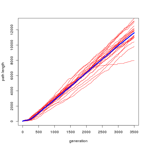
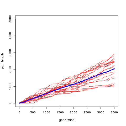
When the full set of methods described in the previous section is applied to the 2D trajectory following task, a linear growth of the length of the learned trajectory over evolutionary time can typically be observed over the full 3500 generations. From Fig. 1, it is apparent that the mean growth of trajectory length is approximately linear although in one run evolution switches to a lower speed at some point. The fitness increase achieved within 50 generations is $168\pm 13$ at generation 1000 (where the second number is the standard error, or uncertainty of the mean), $173\pm 13$ at generation 2000, and $188\pm 16$ at generation 3000. There are no significant pairwise differences between these values when using a Wilcoxon rank sum test, so no significant deviation from linear growth can be found. Overall, a trajectory length of $11604\pm 286$ time steps is reached on average, which corresponds to having adapted to about 387 segments, or 386 potential direction changes.

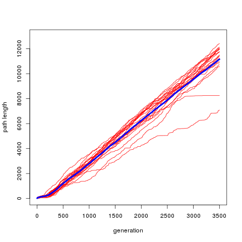
The fact that all path segments have a length of 30 time steps might seem to simplify the task somewhat. If segment lengths are drawn from a uniform distribution between 10 and 50, average trajectory length reaches $11154\pm 292$ (Fig. 2). This is not significantly different ($p=0.31$, Wilcoxon rank sum test).

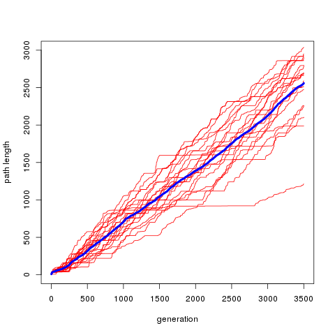
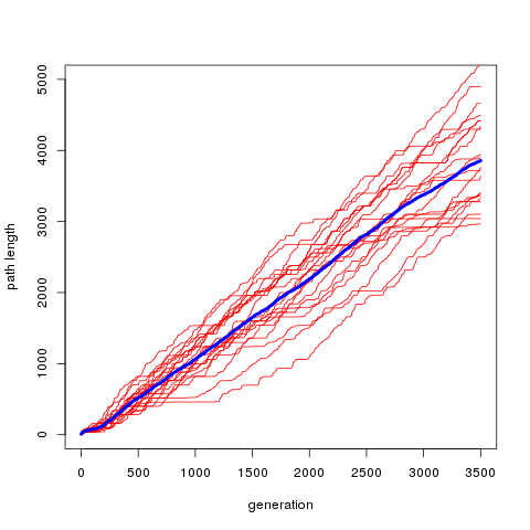
For the 3D trajectory following task, a performance of $2259\pm 97$ is reached, which corresponds to 75 segments on average. It can be seen from Fig. 3 that the mean growth of trajectory length is still approximately linear, but individual runs undergo periods of stagnation, from which they recover sooner or later. By increasing the population size to 1000 (Fig. 4), periods of stagnation become shorter and the performance increases to $3858\pm 147$. When tackling the nonholonomic 3D trajectory following task using a population size of 1000, a performance of $2051\pm 137$ is reached (Fig. 5).

These experiments make it plausible to assume that using the methods presented here, it is indeed possible to evolve trajectories of arbitrary length — or at least very long length — in linear generation time. The observed periods of stagnation do not seem to take away from the linearity as their frequency and duration do not change in an obvious way over the observed number of generations. Furthermore, it is possible to decrease stagnation by increasing the population size. Further experiments (results not shown) using the 2D task and smaller population sizes confirm this as the frequency and duration of stagnation periods increases in a similar way to the way they change between Figs. 4 and 3.

Because trajectory length grows approximately linearly, it makes sense to calculate the speed at which evolution injects information about the trajectory into the population as done previously (Inden and Jost,, 2015). As mentioned above, there are on average 386 decisions about the direction learned within 3500 generations, and for each of them, there are 16 possible directions. So we have $\log_{2}16\cdot\frac{386}{3500}\approx 0.44$ bit / generation. According to Kimura, (1961) and Worden, (1995), the maximally attainable speed for a selection of 5% should be $\log_{2}\frac{1}{0.05}\approx 4.3$ bit / generation. Furthermore, that theory predicts that speed grows logarithmically with selection strength, but is not correlated to population size. We found in further experiments that a trajectory length of $9340\pm 251$ is reached for a selection of 10%, and $6432\pm 183$ for a selection of 20%. Taking the logarithms of the speed ratios for the 5% vs. 10% and 10% vs. 20% configurations, we get 0.31 and 0.54, respectively, which means that the speed grows less than logarithmically with selection strength. From the experiments with different population sizes mentioned above, it follows that there is also a correlation between population size and speed. These observations all indicate that the speed of evolution is limited by the availability of suitable mutations rather than by selection in these experiments. Increasing the population size obviously increases the number of mutated offspring that a selected individual will have and therefore has a direct influence on the speed limiting factor.

3.2 The contribution of individual features to performance

Figure 6: Growth of trajectory length over evolutionary time. Mean and uncertainty of the mean are shown for a standard configuration (black), a configuration without freezing of previously evolved structure (blue), a configuration without temporal scaffolding (green), and a configuration without mutations that create new connections to outputs (red).

Figure 7: Growth of trajectory length over evolutionary time. Mean and uncertainty of the mean are shown for a standard configuration (black, mostly behind green), a configuration with tanh output function (blue), a configuration with mean output function (red), and a standard configuration with the additional possibility to have hidden nodes with sine transfer function (green).

Figure 8: Growth of trajectory length over evolutionary time. Mean and uncertainty of the mean are shown for a standard configuration (black), a CTRNN configuration (blue), a standard configuration without temporal scaffolding (green, barely visible behind red), and a CTRNN configuration without temporal scaffolding (red).

Figure 9: Growth of trajectory length over evolutionary time. Mean and uncertainty of the mean are shown for a standard configuration (black), a NEAT configuration with truncation selection (blue), and a NEAT configuration with speciation selection (green).

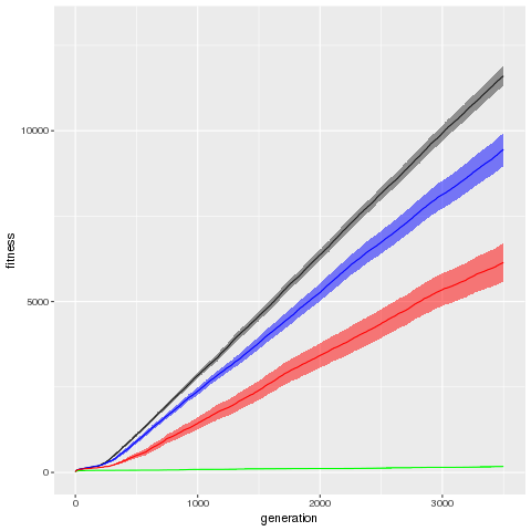
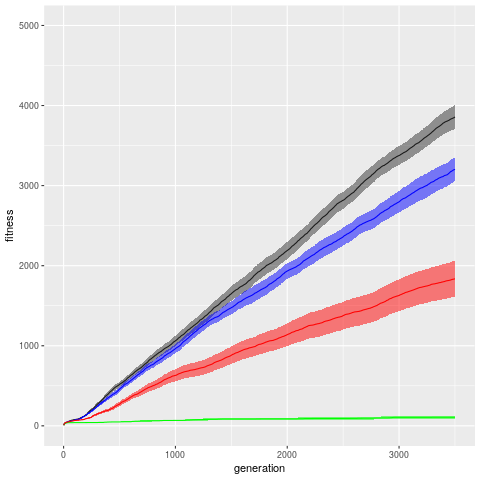
As argued in the introduction to this paper, freezing of previously evolved structure should be an important factor enabling sustained complexification. As shown in Fig. 6, performance indeed becomes significantly worse without this technique ($p<0.001$, Wilcoxon rank sum test), but it is still at 81% of the original performance. Without mutations that create new pathways to output, performance goes down to 53%. Without temporal scaffolding, there is barely any complexification at all.

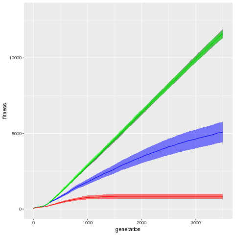
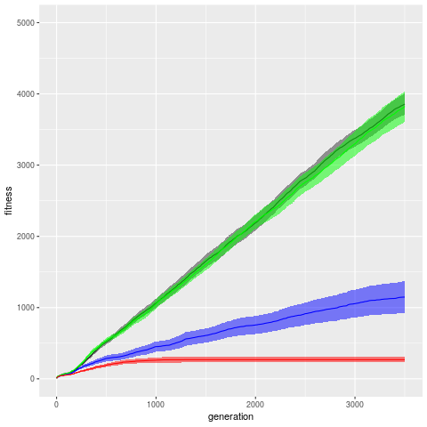
Fig. 7 shows the importance of choosing a homogeneous transfer function for the outputs. When using a hyperbolic tangent function instead of a sine function, average performance goes down to 44%. If the mean function is used, average performance drops to 7%. If evolution can use the sine transfer function for hidden nodes in addition to for outputs, there is no significant difference to the standard method ($p=0.81$, Wilcoxon rank sum test). This supports the idea that the advantage of using the sine function is really in avoiding output saturation and not in any increased evolvability conferred by using the function as such.

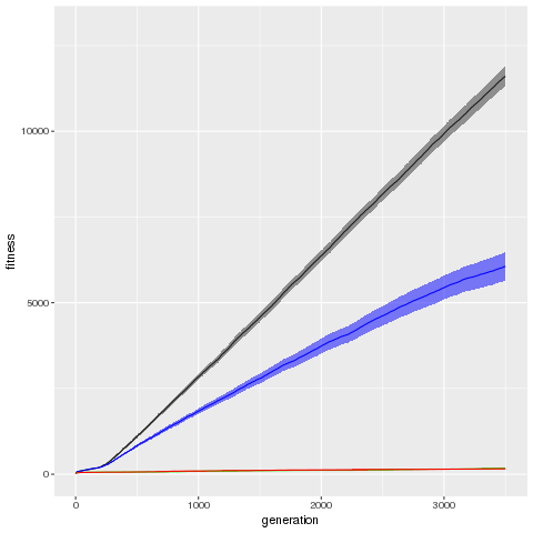
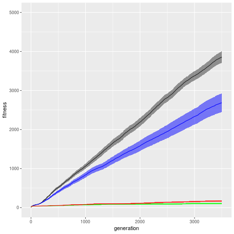
Fig. 8 shows results on methods to generate the temporal dynamics necessary for trajectory following in the neural networks. For this task and with the technical details as specified in this paper, no advantages can be found for using continuous-time recurrent neural network, i.e., networks where the individual neurons change their states slowly as determined by evolved time constants. When used with temporal scaffolding, adding this feature leads to a drop in average performance to 52%, while without temporal scaffolding, both normal and continuous-time networks perform badly with no significant difference ($p=0.63$).

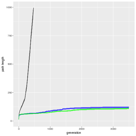
Fig. 9 shows how the method proposed here compares to standard NEAT and a variant thereof that uses the same strong truncation selection as the standard configuration. These reach performances of $111\pm 6$ and $120\pm 7$, respectively. This means that using all the methods presented here increases the performance on the trajectory following task by a factor of 105 as compared to standard NEAT within 3500 generations. Because NEAT leads to stagnation, this factor can be assumed to increase if evolution lasts for more generations.

Figure 10: Growth of trajectory length for the 3D task over evolutionary time. Mean and uncertainty of the mean are shown for a standard configuration (black), a configuration without freezing of previously evolved structure (blue), a configuration without temporal scaffolding (green), and a configuration without mutations that create new connections to outputs (red).

Figure 11: Growth of trajectory length for the 3D task over evolutionary time. Mean and uncertainty of the mean are shown for a standard configuration (black, mostly behind green), a configuration with tanh output function (blue), a configuration with mean output function (red), and a standard configuration with the additional possibility to have hidden nodes with sine transfer function (green).

Figure 12: Growth of trajectory length for the 3D task over evolutionary time. Mean and uncertainty of the mean are shown for a standard configuration (black), a CTRNN configuration (blue), a standard configuration without temporal scaffolding (green), and a CTRNN configuration without temporal scaffolding (red).

Figure 13: Growth of trajectory length for the 3D task over evolutionary time. Mean and uncertainty of the mean are shown for a standard configuration (black), a NEAT configuration with truncation selection (blue), and a NEAT configuration with speciation selection (green).

Finally, as shown in Figs. 10 – 13, similar conclusions regarding the contribution of individual features of the method can be drawn if the experiments are repeated for the 3D trajectory following task and a population size of 1000.

3.3 Structure and function of an evolved neural network

Figure 14: Trajectory of the highest performing individual from the best run. Green: optimal trajectory; blue: actual trajectory. Both start at (0, 0).

Figure 15: The topology of the highest performing individual. Inner ring: inputs; outer ring: hidden neurons. Outputs are shown at the bottom. Connections to outputs are shown in red, while all other connections are drawn in gray. A spoke-like pattern between inputs and hidden neurons and an absence of long range connections are the dominant visible features at that scale. Image created using Cytoscape (Shannon et al.,, 2003).

Figure 16: Magnification of a part in the lower right section of the network from Fig. 15, starting with the first hidden neuron and then proceeding anticlockwise. Some recurrent connections as well as medium range connections between neurons are visible at this scale.

Figure 17: Number of connections in the highest performing individual that go from a neuron to another neuron, where the neuron numbers are assigned according to historical order (i.e., when they arose by mutation).

Figure 18: The average number of connections going from neurons (sorted in historical order and averages taken over groups of 10 neurons each) to outputs for the highest performing individual.

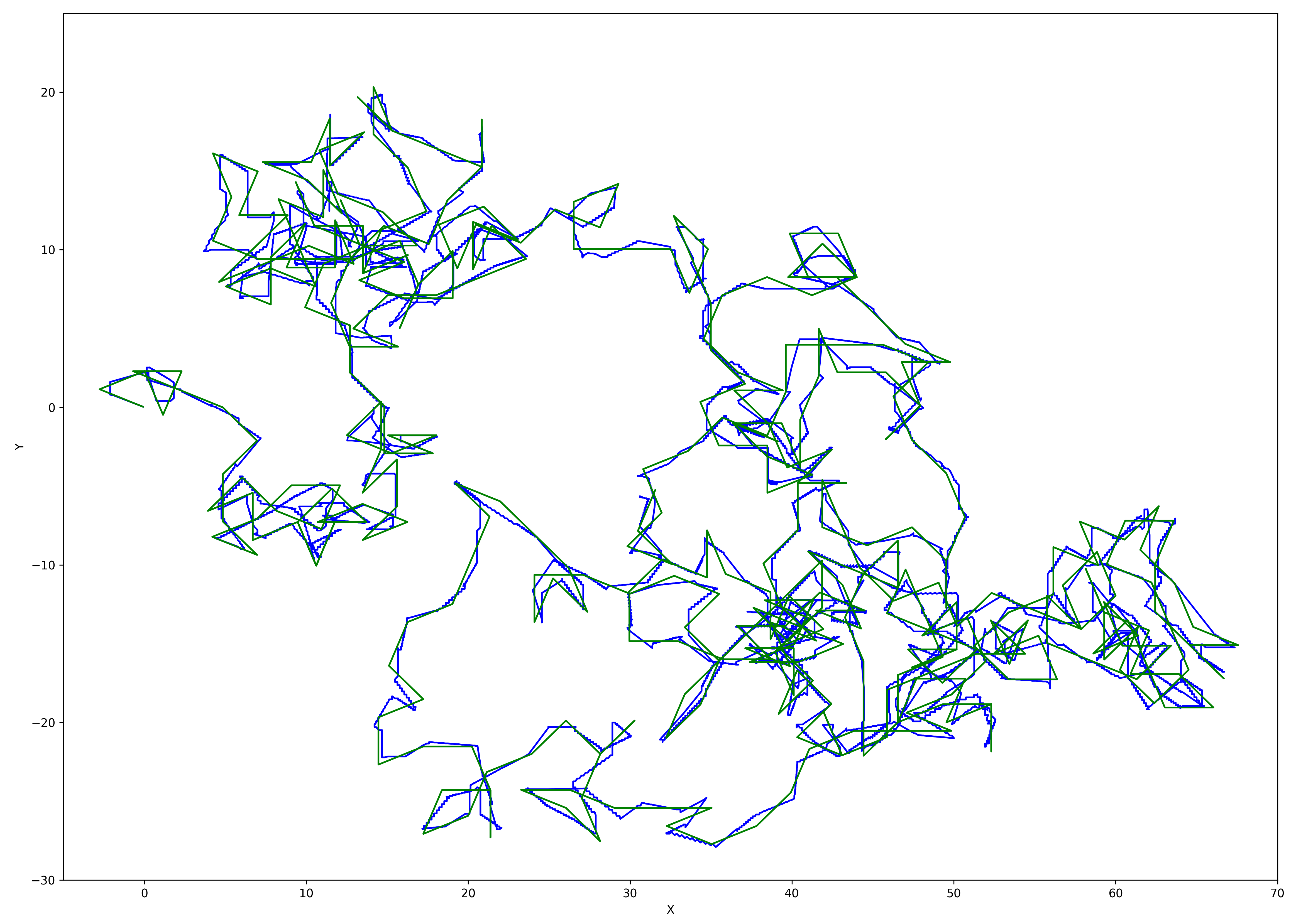
The trajectory of an evolved individual from the best run can be seen in Fig. 14. With the way the fitness function is designed, the individual can get off the original trajectory as long as it is not too far. If a higher accuracy than that is desired, it is possible to scale the whole task, i.e., decrease both the survival radius and the speed with which the individuals and the target point can move. That way, higher accuracy would be achieved at the expense of speed. If only the survival radius is decreased, the task will get more difficult. We expect that this could be compensated for by a larger population size.

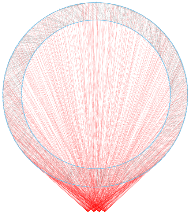
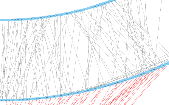
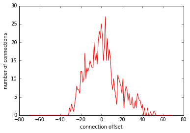
The network of the best individual consists of 676 network inputs (675 of which are scaffolding inputs), 733 neurons, 4 outputs, 1301 connections from input to neurons, 710 connections between neurons, and 816 connections to output. Given that this particular neural network has been adapted to follow 449 segments of the trajectory, it follows that on average 1.6 neurons are used per segment. The low connection to neuron ratio suggests that the network consists of relatively independent modules. Indeed, if network inputs and outputs are removed, the remaining network has 139 connected components, with 5.3 neurons per component on average. This is due to the rareness of medium range connections and absence of long range connections between neurons, which can be easily seen in Figs. 15 and 16. Fig. 17 confirms the visual impression by providing the distribution of internal connections within the network. Also, given that a scaffolding input is active for 20 time steps and a segment for 30 time steps, we would expect $\left\lceil 449\cdot\frac{30}{20}\right\rceil=674$ scaffolding inputs to be present, with a slightly higher number being possible because 5 scaffolding inputs are added to the system in one step whenever necessary as described above. The evolved network conforms to this expectation.

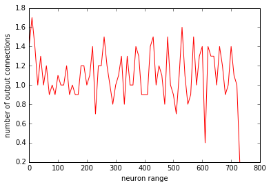
Fig. 18 shows that the number of connections to outputs does not change with the evolutionary age of a neuron except for the very oldest and very youngest neurons. The former exception might be related to the slower speed of evolution in the first few hundred generations (Fig. 1), whereas the latter is because those parts of the network are still under active evolution. In summary, the network structure shows that our methods have achieved the desired stationarity property to a high degree.

4 Conclusions and future work

One conclusion following from the experiments is that the types of neural networks that are often used in evolutionary robotics experiments are not very evolvable. Adding a new kind of mutation and changing the transfer functions of outputs brings some improvement, but the greatest improvement occurs when scaffolding is used. It seems that standard neural networks are not good at producing varied behavior over time — at least not in a way that is easily accessible for evolution. That raises the question whether there might be any sets of building blocks that are more evolvable than neural networks and at the same time reasonable abstractions of biological building blocks. Previous work has used spiking neural networks, compositional pattern producing networks, and finite state automata among others as alternative models (DiPaolo,, 2002; Floreano et al.,, 2005; Florian,, 2006; Stanley,, 2007; Riano and McGinnity,, 2012). As was demonstrated here, using neural networks augmented by scaffolding might be another option. One could argue that various external and internal processes could provide scaffolds for evolution in natural environments, which are typically much richer than artificial environments (Banzhaf et al.,, 2006).

The evolutionary process achieved here is one of sustained rapid complexification without any branching. This can be very useful for technical applications, but we would not argue that this is the normal mode of evolution. Indeed, various authors have argued that there is no general driven trend towards more complexity during evolution (McShea,, 1996; Miconi,, 2008). If anything, one might think that such a dynamics could arise locally for a limited time. Obviously, total freezing of previously evolved structure is also not a biologically plausible assumption. It might be interesting to try to find possible biologically more plausible mechanisms that could approximate the dynamics studied here for some evolutionary time using a task similar to the one described here as a benchmark.

As argued in Inden, (2012), the evolutionary process set up here can be argued to be an instance of open-ended evolution according to the formal definition given by Bedau et al., (1998). However, since that early work, the scientific debate on open-ended evolution has moved on. Many authors now consider the emergence of new evolutionary units and levels, and/or the continuing presence of highly diverse solution candidates, as hallmarks of open-ended evolution (Taylor et al.,, 2016; Banzhaf et al.,, 2016). We have not addressed those issues here, which is why we would describe the observed dynamics as sustained complexification instead.

The paths to be learned here are essentially random sequences, therefore evolution proceeds towards behaviors with higher algorithmic or Kolmogorov complexity (Li and Vitányi,, 1997). Many researchers are more concerned with whether the complexity concerned with structural regularities can increase during evolution (Ay et al.,, 2011). We do not address this question here. The growth of algorithmic complexity of the genotype and phenotype seems to be a necessary, but not sufficient, condition for the evolution of interesting complex behaviors. The point here is not to argue that any task of interest might require that the complexity of solutions grows forever. It is rather that many problems of interest seem to require solutions of an algorithmic complexity that is unknown in advance, but most likely higher than what can be achieved with current methods. For these problems, techniques that can achieve a sustained growth of complexity should be useful.

A related concern is that learning normally entails the ability to solve previously unseen tasks that are similar to tasks seen during training. Our evolved solutions do not have this ability in general. For example, imagine a new path where only the direction of a single segment would be changed. This could be sufficient to increase the distance between the individual and its path so much that it would die, rendering all skills for subsequent path segments useless. Furthermore, because the structure bringing about the movement at this time would likely already be frozen, evolution would not be able to re-adapt the individual within a few generations. Therefore, it is probably more accurate to say that evolution adapts individuals towards following the path instead of saying that the path has been learned. That said, it seems that much of the generalization ability, or ability to perform well despite slight environmental change, in natural organisms results either from developmental processes that are dependent on the environment (Sultan,, 2007), or from learning mechanisms within their neural networks (Downing,, 2007). Therefore, we suggest that the proper role of artificial evolution in creating robot controllers might be to build structures that are capable of both performing some rather fixed action patterns (of which the tasks studied here provide abstract instances) and learning more advanced and flexible behavior based on these skills during their lifetime. Unsurprisingly, the evolution of plastic neural networks is an active research area (Floreano et al.,, 2008; Soltoggio et al.,, 2008; Tonelli and Mouret,, 2013). The concept of a fixed action pattern was introduced in Lorenz (1935; 1981). It refers to a complex spatio-temporal pattern of behavior that arises as an instinctive response to a stimulus. Once elicited, it typically lasts much longer than the stimulus and executes independently of further external input. Examples include various escape behaviors, courtship and aggression signals, and ecdysis related behavior in insects. Although the concept has been criticized in later research with respect to the assumed full independence from external stimuli in some of the mentioned examples, it continues to be a useful concept in both biology and robotics (Lawrence and Watson,, 2002; Watt and Joss,, 2003; Borst,, 2014; Kim et al.,, 2015; Prescott et al.,, 2006). Our methods can create fixed action patterns of high complexity. If the scaffolding inputs are made dependent on the environment, these action patterns can even become flexible to a degree.

From a technical perspective, one might be most interested in the question of how well the method can be used on other tasks. The tasks studied in this article represent tasks that require a complex fixed pattern of movement to be executed. This would also include trajectories in non-physical spaces, for example the generation of complex sound patterns, or the execution of a developmental program by a simple model of a genetic regulatory network in order to create a complex phenotype (Hinman et al.,, 2003; Stanley and Miikkulainen,, 2003; Doursat et al.,, 2013). One possible criticism regarding limitations of the method would be to think of a robotics-related version of a trap fitness function, where following a certain path is required, but once a certain point has been reached, the path to be followed earlier in order to achieve the highest fitness changes. These kinds of tasks could not be solved by our method in its pure form. However, one needs to consider three points: (1) It is an open question whether any of these tasks would actually correspond to any useful instinctive behavior that can be observed in natural organisms, or would be useful for artificial organisms. Evolution cannot solve all kinds of problems anyway (Barton and Partridge,, 2000), and incrementality — building new function on top of old function instead of changing the old function — is a key feature of many evolved solutions. (2) Some kinds of these problems might be successfully tackled by using diversity preserving selection mechanisms, perhaps together with recombination, and developing these is an orthogonal research direction in evolutionary robotics (Pugh et al.,, 2016). The resulting methods could possibly be combined with the methods presented here. (3) While we freeze all but the most recently evolved structure here, an experimenter with some prior understanding of the task to be solved could inject that knowledge into the evolutionary process by freezing different parts of the structure at different evolutionary times.

The tasks studied here, and the task studied in Inden and Jost, (2013), are all tasks that require certain behavior at certain points in time. Other tasks might require certain behaviors in certain situations, where situations might occur repeatedly and be determined by various factors in the environment. In that case, one could still use the same methods, including the incremental provision of inputs, but just use inputs that indicate the situation instead of the time. This input could come from sensors or even from subnetworks that have previously been evolved to recognize certain situations.

The experiments on trajectory following in higher dimensional spaces seem to indicate that performance goes down as the number of outputs increases. This is another limitation of the presented method. It is understandable given the large increase in local search space that the addition of only one output incurs (in principle, all neurons could be connected to that output). If there are more than just a few outputs, then perhaps one can use incremental provision of outputs in a similar fashion to the way inputs are provided incrementally if the task allows to learn their behavior separately. Of course, tasks with many outputs have been previously solved using methods that exploit the geometric regularities of the tasks (Stanley et al.,, 2009; Inden et al.,, 2012) — another orthogonal research direction whose results could be easily combined with the methods presented here. For example, large and regular HyperNEAT networks are generated by an underlying network — one could apply the methods discussed here onto that underlying network. In NEATfields, applying our methods would also be straightforward; the main task would be to specify how those additional mutation operators that change the parameters of the design patterns interact with the freezing of previously evolved structure.

Another limitation of the approach presented here is that while the number of necessary generations depends linearly on the trajectory length, the run time of the algorithm is at least quadratic. That is because the maximum and average lengths of trajectories achieved before individuals die also grow linearly over the generations. (An even higher computational complexity is expected because the size of the neural networks also increases over time.) With our implementation and available hardware, run times of up to two weeks were typical for standard configurations. That said, speedups could be achieved by parallelizing fitness evaluation. It would also be possible to divide a longer trajectory into several shorter ones, evolve trajectory following for each one separately, and then evolve or hand design a mechanism that ensures that the right subnetworks are active at each time step. If the length of the individual pieces of the trajectory remained constant and ignoring any effort for the arbitration mechanisms, that would result in a linear run time.

Based on these thoughts and the results of the experiments presented, we conclude that the methods presented here — freezing of previously evolved structure, temporal scaffolding, a homogeneous transfer function for output nodes, and mutations that create new pathways to outputs — might become essential ingredients of future methods that are used to evolve neural networks for robot control and other tasks.

Declarations of interest:

none. This research did not receive any specific grant from funding agencies in the public, commercial, or not-for-profit sectors.

References

- Ay et al., (2011) Ay, N., Olbrich, E., Bertschinger, N., and Jost, J. (2011). A geometric approach to complexity. Chaos, 21:037103.
- Banzhaf et al., (2016) Banzhaf, W., Baumgaertner, B., Beslon, G., Doursat, R., Foster, J. A., McMullin, B., de Melo, V. V., Miconi, T., Spector, L., Stepney, S., and White, R. (2016). Defining and simulating open-ended novelty: requirements, guidelines, and challenges. Theory in Biosciences, 135:131–161.
- Banzhaf et al., (2006) Banzhaf, W., Beslon, G., Christensen, S., Foster, J. A., Képès, F., Lefort, V., Miller, J. F., Radman, M., and Ramsden, J. J. (2006). From artificial evolution to computational evolution: a research agenda. Nature Reviews Genetics, 7:729–735.
- Barton and Partridge, (2000) Barton, N. and Partridge, L. (2000). Limits to natural selection. BioEssays, 22:1075–1084.
- Bedau et al., (1998) Bedau, M. A., Snyder, E., and Packard, N. H. (1998). A classification of long-term evolutionary dynamics. In et al., C. A., editor, Artificial Life VI.
- Beer, (2006) Beer, R. (2006). Parameter space structure of continuous-time neural networks. Neural Computation, 18:3009–3051.
- Beer and Gallagher, (1992) Beer, R. D. and Gallagher, J. C. (1992). Evolving dynamical neural networks for adaptive behavior. Adaptive Behavior, 1:91–122.
- Borst, (2014) Borst, A. (2014). Fly visual course control: behaviour, algorithms and circuits. Nature Reviews Neuroscience, 14:590 – 599.
- DiPaolo, (2002) DiPaolo, E. (2002). Spike timing dependent plasticity for evolved robots. Adaptive Behavior, 10:243–263.
- Doncieux et al., (2015) Doncieux, S., Bredeche, N., Mouret, J.-B., and Eiben, A. E. (2015). Evolutionary robotics: what, why, and where to. Frontiers in Robotics and AI.
- Doursat et al., (2013) Doursat, R., Sayama, H., and Michel, O. (2013). A review of morphogenetic engineering. Natural Computing, 12:517–535.
- Downing, (2007) Downing, K. L. (2007). Neuroscientific implications for embodied and situated artificial intelligence. Connection Science, 19(1):75–104.
- Eiben and Smith, (2015) Eiben, A. E. and Smith, J. E., editors (2015). Introduction to Evolutionary Computing. Springer-Verlag.
- Eigen, (1971) Eigen, M. (1971). Selforganization of matter and evolution of biological macromolecules. Naturwissenschaften, 58:465–523.
- Fahlman and Lebiere, (1990) Fahlman, S. E. and Lebiere, C. (1990). The cascade-correlation learning architecture. In Touretzky, D. S., editor, Advances in Neural Information Processing Systems, volume 2, pages 524–532. Morgan Kaufman.
- Field et al., (2016) Field, M., Stirling, D., Pan, Z., and Naghdy, F. (2016). Learning trajectories for robot programing by demonstration using a coordinated mixture of factor analyzers. IEEE Transactions on Cybernetics, 46(3):706 – 717.
- Floreano et al., (2008) Floreano, D., Dürr, P., and Mattiussi, C. (2008). Neuroevolution: from architectures to learning. Evolutionary Intelligence, 1:47–62.
- Floreano et al., (2005) Floreano, D., Zufferey, J. C., and Nicoud, J.-D. (2005). From wheels to wings with evolutionary spiking circuits. Artificial Life, 11:121–138.
- Florian, (2006) Florian, R. V. (2006). Spiking neural controllers for pushing objects around. In International Conference on Simulation of Adaptive Behavior, pages 570–581. Springer.
- Geman et al., (1992) Geman, S., Bienenstock, E., and Doursat, R. (1992). Neural networks and the bias/variance dilemma. Neural Computation, 4:1 – 58.
- Gomez et al., (2012) Gomez, F., Koutník, J., and Schmidhuber, J. (2012). Compressed network complexity search. In Proceedings of the 12th International Conference on Parallel Problem Solving from Nature.
- Green, (2006) Green, C. (2006). SharpNEAT. http://sharpneat.sourceforge.net.
- Hinman et al., (2003) Hinman, V. F., Nguyen, A. T., Cameron, R. A., and Davidson, E. H. (2003). Developmental gene regulatory network architecture across 500 million years of echinoderm evolution. Proceedings of the National Academy of Sciences, 100(23):13356 – 13361.
- Hülse et al., (2004) Hülse, M., Wischmann, S., and Pasemann, F. (2004). Structure and function of evolved neuro-controllers for autonomous robots. Connection Science, 6(4):249–266.
- Inden, (2012) Inden, B. (2012). Open-ended coevolution and the emergence of complex irreducible functional units in iterated number sequence games. In Proceedings of the 14th annual conference on genetic and evolutionary computation.
- Inden et al., (2012) Inden, B., Jin, Y., Haschke, R., and Ritter, H. (2012). Evolving neural fields for problems with large input and output spaces. Neural Networks, 28:24–39.
- Inden and Jost, (2013) Inden, B. and Jost, J. (2013). Neural agents can evolve to reproduce sequences of arbitrary length. In Proceedings of the European Conference on Artificial Life.
- Inden and Jost, (2015) Inden, B. and Jost, J. (2015). Effects of several bioinspired methods on the stability of coevolutionary complexification. In Proceedings of the 2015 IEEE Symposium Series on Computational Intelligence.
- Kim et al., (2015) Kim, D.-H., Han, M.-R., Lee, G., Lee, S. S., Kim, Y.-J., and Adams, M. E. (2015). Rescheduling behavioral subunits of a fixed action pattern by genetic manipulation of peptidergic signaling. PLoS Genetics, 11(9):e1005513.
- Kimura, (1961) Kimura, M. (1961). Natural selection as the process of accumulating genetic information in adaptive evolution. Genetical Research, 2(1):127–140.
- Koutník et al., (2010) Koutník, J., Gomez, F., and Schmidhuber, J. (2010). Evolving neural networks in compressed weight space. In Proceedings of the Genetic and Evolutionary Computation Conference.
- Laumond et al., (1998) Laumond, J. P., Sekhavat, S. S., and Lamiraux, F. (1998). Guidelines in nonholonomic motion planning. In Laumond, J., editor, Robot motion planning and control, Lecture Notes in Control and Information Sciences. Springer.
- Lawrence and Watson, (2002) Lawrence, K. A. and Watson, W. H. (2002). Swimming behavior of the Nudibranch Melibe leonina. The Biological Bulletin, 203(2):144–151.
- Li and Vitányi, (1997) Li, M. and Vitányi, P. (1997). An introduction to Kolmogorov complexity and its applications. Springer.
- Liu et al., (2018) Liu, H., Simonyan, K., Vinyals, O., Fernando, C., and Kavukcuoglu, K. (2018). Hierarchical representations for efficient architecture search. In Proceedings of the Sixth International Conference on Learning Representations.
- Lorenz, (1935) Lorenz, K. (1935). Der Kumpan in der Umwelt des Vogels. Journal of Ornithology, 83:289 – 413.
- Lorenz, (1981) Lorenz, K. (1981). The foundations of ethology. Springer-Verlag.
- Martincorena et al., (2012) Martincorena, I., Seshasayee, A. S. N., and Luscombe, N. M. (2012). Evidence of non-random mutation rates suggests an evolutionary risk management strategy. Nature, 485:95–98.
- McShea, (1996) McShea, D. W. (1996). Metazoan complexity and evolution: Is there a trend? Evolution, 50(2):477–496.
- Miconi, (2008) Miconi, T. (2008). Evolution and complexity: The double-edged sword. Artificial Life, 14:325–344.
- Miikkulainen et al., (2019) Miikkulainen, R., Liang, J., Meyerson, E., Rawal, A., Fink, D., Francon, O., Raju, B., Shahrzad, H., Navruzyan, A., Duffy, N., and Hodjat, B. (2019). Evolving deep neural networks. In Kozma, R., Alippi, C., Choe, Y., and Morabito, F. C., editors, Artificial Intelligence in the Age of Neural Networks and Brain Computing, pages 293 – 312. Academic Press.
- Nolfi and Floreano, (2000) Nolfi, S. and Floreano, D. (2000). Evolutionary Robotics — The Biology, Intelligence, and Technology of Self-Organizing Machines. MIT Press.
- Poli et al., (2008) Poli, R., Langdon, W. B., and McPhee, N. F. (2008). A Field Guide to Genetic Programming. Published via http://lulu.com.
- Prescott et al., (2006) Prescott, T. J., González, F. M. M., Gurney, K., Humphries, M. D., and Redgrave, P. (2006). A robot model of the basal ganglia: Behavior and intrinsic processing. Neural Networks, 19:31 – 61.
- Pugh et al., (2016) Pugh, J. K., Soros, L. B., and Stanley, K. O. (2016). Quality diversity: A new frontier for evolutionary computation. Frontiers in Robotics and AI.
- Real et al., (2017) Real, E., Moore, S., Selle, A., Saxena, S., Suematsu, Y. L., Tan, J., Le, Q. V., and Kurakin, A. (2017). Large-scale evolution of image classifiers. In Proceedings of the 34th International Conference on Machine Learning.
- Rempis and Pasemann, (2012) Rempis, C. W. and Pasemann, F. (2012). Evolving variants of neuro-control using constraint masks. In SAB, pages 187–197. Springer.
- Riano and McGinnity, (2012) Riano, L. and McGinnity, M. T. (2012). Automatically composing and parameterizing skills by evolving finite state automata. Robotics and Autonomous Systems, 60:639–650.
- Rusu et al., (2016) Rusu, A. A., Rabinowitz, N. C., Desjardins, G., Soyer, H., Kirkpatrick, J., Kavukcuoglu, K., Pascanu, R., and Hadsell, R. (2016). Progressive neural networks. CoRR, abs/1606.04671.
- Schliebs and Kasabov, (2013) Schliebs, S. and Kasabov, N. (2013). Evolving spiking neural network — a survey. Evolving Systems, 4(2):87 – 98.
- Schmidhuber, (2015) Schmidhuber, J. (2015). Deep learning in neural networks: An overview. Neural Networks, 61:85–117.
- Shannon et al., (2003) Shannon, P., Markiel, A., Ozier, O., Baliga, N. S., Wang, J. T., Ramage, D., Amin, N., Schwikowski, B., and Ideker, T. (2003). Cytoscape: a software environment for integrated models of biomolecular interaction networks. Genome research, 13(11):2498–2504.
- Soltoggio et al., (2008) Soltoggio, A., Bullinaria, J., Mattiussi, C., Dürr, P., and Floreano, D. (2008). Evolutionary advantages of neuromodulated plasticity in dynamic, reward- based scenarios. In Proceedings of the 11th International Conference on Artificial Life.
- Stanley, (2007) Stanley, K. (2007). Compositional pattern producing networks: A novel abstraction of development. Genetic Programming and Evolvable Machines, pages 131–162.
- Stanley and Miikkulainen, (2002) Stanley, K. and Miikkulainen, R. (2002). Evolving neural networks through augmenting topologies. Evolutionary Computation, 10:99–127.
- Stanley and Miikkulainen, (2003) Stanley, K. and Miikkulainen, R. (2003). A taxonomy for artificial embryogeny. Artificial Life, 9:93–130.
- Stanley et al., (2009) Stanley, K. O., D’Ambrosio, D. B., and Gauci, J. (2009). A hypercube-based encoding for evolving large-scale neural networks. Artificial Life, 15:185–212.
- Stanley and Miikkulainen, (2004) Stanley, K. O. and Miikkulainen, R. (2004). Competitive coevolution through coevolutionary complexification. Journal of Artificial Intelligence Research, 21:63–100.
- Sultan, (2007) Sultan, S. E. (2007). Development in context: the timely emergence of eco-devo. TRENDS in Ecology and Evolution, 22:575–582.
- Taylor et al., (2016) Taylor, T., Bedau, M., Channon, A., Ackley, D., Banzhaf, W., Beslon, G., Dolson, E., Froese, T., Hickinbotham, S., Ikegami, T., McMullin, B., Packard, N., Rasmussen, S., Virgo, N., Agmon, E., Clark, E., McGregor, S., Ofria, C., Ropella, G., Spector, L., Stanley, K. O., Stanton, A., Timperley, C., Vostinar, A., and Wiser, M. (2016). Open-ended evolution: Perspectives from the OEE workshop in York. Artificial Life, 22:408–423.
- Terekhov et al., (2015) Terekhov, A. V., Montone, G., and O’Regan, J. K. (2015). Knowledge transfer in deep block-modular neural networks. In Conference on Biomimetic and Biohybrid Systems, pages 268–279. Springer.
- Togelius, (2004) Togelius, J. (2004). Evolution of a subsumption architecture neurocontroller. Journal of Intelligent and Fuzzy Systems, 15:15–20.
- Tonelli and Mouret, (2013) Tonelli, P. and Mouret, J.-B. (2013). On the relationships between generative encodings, regularity, and learning abilities when evolving plastic artificial neural networks. PLoS ONE, 8(11):e79138.
- Vakanski et al., (2012) Vakanski, A., Mantegh, I., Irish, A., and Janabi-Sharifi, F. (2012). Trajectory learning for robot programming by demonstration using hidden Markov model and dynamic time warping. IEEE Transactions on Systems, Man, and Cybernetics — Part B: Cybernetics, 42(4):1039 – 1052.
- Watt and Joss, (2003) Watt, M. and Joss, J. (2003). Structure and function of visual displays produced by male jacky dragons, Amphibolurus muricatus, during social interactions. Brain, Behaviour and Evolution, 61(4):172 – 183.
- Whiteson et al., (2005) Whiteson, S., Stone, P., Stanley, K. O., Miikkulainen, R., and Kohl, N. (2005). Automatic feature selection in neuroevolution. In Proceedings of the Genetic and Evolutionary Computation Conference.
- Worden, (1995) Worden, R. P. (1995). A speed limit for evolution. Journal of Theoretical Biology, 176:137–152.